
Generalizing Normality: Different Estimation Methods for Skewed Information
by
 , ,
, ,
Diego Carvalho do Nascimento
1,*,† ,
,
Pedro Luiz Ramos
2,† ,
,
David Elal-Olivero
1,†, 
Milton Cortes-Araya
1,† and
Francisco Louzada
2,† 1
Departamento de Matemática, Facultad de Ingeniería, Universidad de Atacama, Copiapó 1530000, Chile
2
Institute of Mathematical Science and Computing, University of São Paulo, São Carlos 13566590, Brazil
*
Author to whom correspondence should be addressed.
†
These authors contributed equally to this work.
Symmetry 2021, 13(6), 1067; https://doi.org/10.3390/sym13061067
Submission received: 6 May 2021
/
Revised: 8 June 2021
/
Accepted: 10 June 2021
/
Published: 15 June 2021
(This article belongs to the Special Issue Symmetric and Asymmetric Bimodal Distributions with Applications)
Abstract
:Normality is the most commonly used mathematical supposition in data modeling. Nonetheless, even based on the law of large numbers (LLN), normality is a strong presumption, given that the presence of asymmetry and multi-modality in real-world problems is expected. Thus, a flexible modification in the normal distribution proposed by Elal-Olivero adds a skewness parameter called Alpha-skew-normal (ASN) distribution, which enables bimodality and fat-tail, if needed, although it is sometimes not trivial to estimate this third parameter (regardless of the location and scale). This work analyzed seven different statistical inferential methods towards the ASN distribution on synthetic data and historical data of water flux from 21 rivers (channels) in the Atacama region. Moreover, the contributions of this paper are related to the estimations of probability surrounding rivers’ flux levels in the surroundings of Copiapó city, which is the most economically important city of the third Chilean region and is known to be located in one of the driest areas on Earth (excluding the North and the South Poles). The results show the competitiveness of the MPS and RADE methods with respect to the MLE method, as well as their excellent performance.
1. Introduction
We live in the Big Data Era, where high volumes and many varieties of data characterization are often noticeable in data lakes. Despite the amount of observation, symmetry and smooth tails are not always observed. These characteristics are natural because we all live in a complex world with nonlinear relations and outliers that describe extreme values, which are more recurrent than easy statistical tools take into account. This new age requires flexible models and different reasoning based on data and information.
A question that is often asked in traditional departments worldwide is: “Are statistical methods becoming old fashioned?”. Sir David Cox [1] explained that the focus is on the relevance and quality of data based on their coverage and representativeness, which provide confidence in the results in spite of the amount of information (large volumes) in a set, which may hold some potentially biased estimates with measurement errors. Efron and Hastie [2] discussed the relation between computer-related inferences and statistical inferences as a system of mathematical logic for guidance and correction that is complemented by large-scale prediction algorithms that are suitable for this new century.
Therefore, complexity is intrinsic to massive amounts of data, where high dimensionality and dynamism are often present [3,4]. Nonetheless, all of the information contained in the acquired data can be extracted by using an estimation method, e.g., with maximum likelihood estimation (MLE); a parametric version of such a method will be supported by a supposed distribution. Parametric approaches can be used to easily interpret patterns by using parameters, enable association across variables, present a low computational cost, and are easier to implement in decision-making systems.
In many cases, the standard MLE may not return desirable results. Other estimation methods that return accurate estimates have been considered, such as estimators based on the least-square function [5], the product of spacing [6,7], or goodness-of-fit statistics [8]. There is not a unique method that performs better in all models, and the performance may depend on the selected parametric form [9,10]. Thus, it is necessary to use an efficient estimation method jointly with a flexible parametric model that covers many data patterns and that sometimes accommodates the asymmetry and multi-modality that may be contained in the data under consideration.
This is the case of meteorological data, which show significant changes, as well as a complex dynamic [11,12]. This field demands extra attention on data-driven models, which are needed in order to incorporate space–time dependence [13], structural changes [14], and extreme values [15]. Moreover, in a parametric world, a model supported by a probabilistic model (which deals with asymmetry and multi-modality [16,17]) is necessary. Thus, this paper was motivated by a case study of the water flux of 21 rivers (channels) in the surroundings of Copiapó city, which is located in the Atacama Desert and is one of the planet’s driest areas. Moreover, we intend to exemplify evidence of the probability densities associated with these events’ empirical distribution by using seven different approaches to statistical inference.
This paper is divided into four parts. Section 2 presents the motivation and details regarding the analyzed data. Section 3 provides the background of the adopted methodology with respect to the elements of statistical inference. Then, Section 4 and Section 5 show the developments related to the methods when implemented on synthetic data and for the analysis of real-world data. Finally, Section 6 discusses the findings based on the obtained results.
2. The Data
The dataset adopted is related to fluviometric records (average monthly flows) from the Atacama Desert region (third-largest region of Chile) in the surroundings of Copiapó city. The historical period of these data is that of the ten years from January 2011 to December 2020; the data are associated with 21 rivers (or stream channels) and were obtained from the Chilean government website called Direccion General de Aguas (Información Oficial Hidrometeorológica y de Calidad de Aguas en Línea).
Historical events revealed the high periodicity of the low water flux of the region. However, cyclical events were also noticeable (such as two rainfall events and defrosting of glaciers/snow in summer, amongst others), creating the expected multi-modality and a large leptokurtosis.
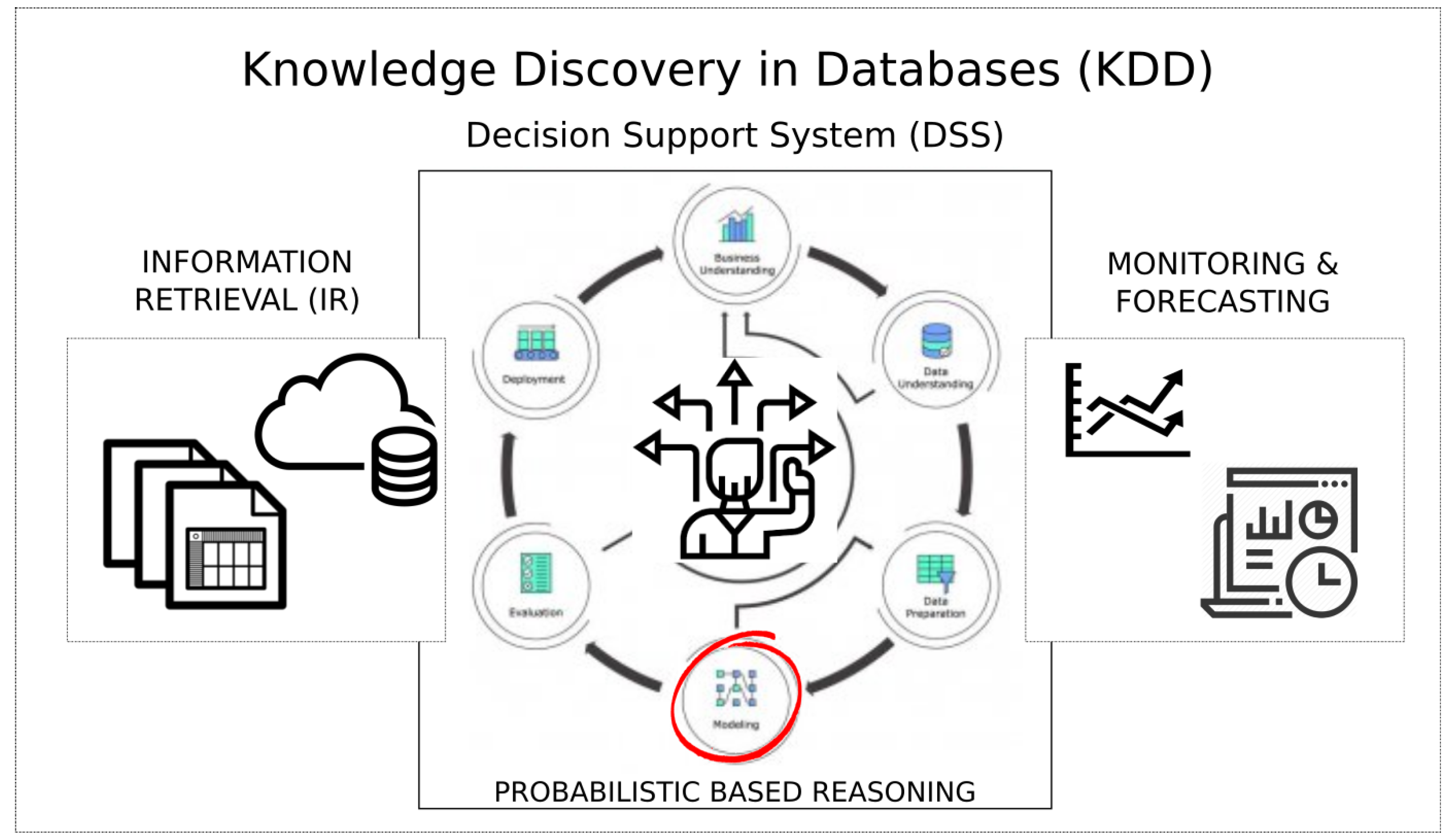
During the processing of information, a decision-support system (DSS) sifts through and analyzes massive amounts of data, compiling comprehensive information that can be used in solving problems and making decisions. Figure 1 presents a flowchart of knowledge discovery in databases (KDD); the process involves information retrieval (IR), the decision-support system (DSS), and monitoring and forecasting.
Thus, the Atacama Desert watershed problem is part of a multi-dimensional study related to the analysis of a circular economy. It is essential to mention that uncertainty is always presented globally (as a measurement error or sample bias, amongst others). Nonetheless, probabilistic reasoning allows one to generalize results through statistical inference procedures.
3. Statistical Inference Elements
3.1. Alpha-Skew-Normal (ASN) Distribution
Let X be a random variable that follows an Alpha-skew-normal (ASN) distribution [18]; then, its probability density function (PDF) is given by
where , , and is the PDF of the standard normal distribution.
The cumulative density function (CDF) is given by
Then, wrapping the ASN density f(x) with the parameters for location () and scale (), that is, the random variable T is defined by for and , this value is given by:
Figure 2 presents different forms of the PDF of the ASN distribution.
The CDF related to Equation (4) is
Given its flexibility, the ASN distribution has been used in data modeling and has been adopted in different fields, such as astronomy [19], the modeling of wind speed [20], and for benchmark data [21]. Figure 2 presents different forms of the PDF of the ASN distribution, assuming, for instance, (location), (scale), and other values for , in order to show the presence of asymmetry and bimodality (incorporating different heights between the modalities).
3.2. Different Estimation Methods for the ASN Distribution
In this subsection, we will discuss seven different estimation methods (maximum likelihood estimation, ordinary and weighted least-square estimate, method of the maximum product of spacings, Cramer–von Mises minimum distance estimators, Anderson–Darling estimators, and right-tail Anderson–Darling estimators) for the parameters (, and ) of the ASN distribution. Table 1 describes the methods used and the authors that proposed these inferential procedures. A comparison that used the cited estimators was presented for other models [22,23,24].
Note that Carl Friedrich Gauss introduced the LSQ in 1822, and it is one of the oldest estimation procedures, although it was only in the paper of Swain et al. [5] that this approach was discussed for a class of non-normal models, and it then became a standard reference when applied in different probability distributions. The additional details related to the estimation of the ASN distribution’s parameters are presented in the following subsections.
3.2.1. Maximum Likelihood Estimation
Maximum likelihood estimation (MLE) is widely used in data analysis; Fisher’s derivation of information inequality was first used for the analysis of variance, and later for the estimation of functions derived from Euler’s relation for homogeneous functions. Despite the fact that historical records of this technique have been widely exposed and defended by Ronald A. Fisher (who likely gained visibility because of his epic fights with Egon S. Pearson), its reasoning dates back to the mid-1700s [28].
Let be a sample of a random sample of size n from . Considering , the maximum likelihood estimators , , and can be obtained by maximizing
with respect to , and . The log-likelihood function of (5) is given by
From the expressions , , , the likelihood equations are
Numerical methods, such as the Newton–Rapshon, method are required in order to find the solution of a nonlinear system. Under mild conditions, the MLEs are asymptotically normally distributed with a joint multivariate normal distribution that is given by
where is the Fisher information matrix given by Elal-Olivero [18], who discussed that the ASN family satisfies these mild conditions.
This methodology is often adopted because of the sufficiency of the MLE, combined with its consistency (which leads to the statistical efficiency) and the fact that asymptotic normality is guaranteed. Next, we will present a series of minimum distance estimations (which are easily applied to estimate consistently unknown parameters) that are designed to reflect the proposed model in order to reproduce the probabilistic structure of the real-world phenomenon under study [29]. Minimum distance estimations provide consistent parameter estimates and are competitive, especially where other methods do not succeed.
3.2.2. Ordinary and Weighted Least-Square Estimates
Consider a random sample of order statistics of size n as , where is not independent of , and is its monotonic function. The least-square (LSQ) estimators , , and for the ASN distribution can be obtained by minimizing the parameters , and :
Thus, the LSQ equations can be obtained by solving the non-linear equations
where
Alternative solutions are obtained through high-precision numerical approximations of for partial derivatives.
Alternatively, the weighted least-squares (WLQ) estimates have been proposed for whenever an efficient method is required with small sets of data. , , and can be obtained by adopting the following minimized equation:
The solutions deviate from those of the non-linear equations:
where , and are given in (13). The WLQ estimation technique is particularly useful whenever one aims to weigh observations in proportion to the equivalence of the error variance for an observation in order to overcome the issue of non-constant variance.
3.2.3. Method of the Maximum Product of Spacings
The maximum product of spacings (MPS) method is a powerful alternative to MLE for estimating unknown parameters of continuous univariate distributions; it aims to maximize the geometric mean of the spacings in the data (differences between the values of the cumulative distribution function at neighborhood data points). Cheng and Amin proposed this method [6,30]—though it was also found independently by Ranneby [7]—as a Kullback–Leibler information approximation measurement. Some desirable properties of the MPS methods, such as their asymptotic efficiency, invariance, and, most importantly, consistency, are held more broadly (under general conditions) than for MLEs [30].
Let us represent the differences between the values of the cumulative distribution functions on their neighborhood data points with the function for as a uniform spacing of a random sample from the ASN distribution, which is defined by and . The constraint of holds. Thus, the MPS estimates , , and can be obtained by maximizing the geometric mean of the spacings:
considering the maximization of this function () by adopting its logarithm as
The estimates of the unknown parameters , , and are obtained by solving the nonlinear equations
where , , and are given, respectively, in Equation (13).
It is important to mention that if , then . Therefore, the MPS estimators are sensitive to closely spaced observations—especially ties. When the ties are due to multiple observations, should be replaced with the corresponding likelihood, , because .
Under mild conditions, for the ASN distribution, the MPS estimators are asymptotically normally distributed with a joint trivariate normal distribution given by
3.2.4. The Cramer–von Mises Minimum Distance Estimators
Alternatively, an estimator that requires no assumptions about the distributions’ parametric form, the Cramer–von Mises estimator (CME), is based on the difference between the estimates of the cumulative distribution function and the empirical distribution function [31,32]. These estimators operate based on the minimum distance across the “true” distribution (observed) and the “modeled” distribution (adjusted) through the maximum goodness of fit.
Macdonald [26] showed that the bias of the estimator in the CME presents smaller distances than those of other minimum distance estimators. The Cramer–von Mises estimates , , and of the parameters , , and are obtained through minimization with
Thus, these estimates are also obtained by solving the non-linear equations:
where , and are given, respectively, in Equation (13).
3.2.5. The Anderson–Darling and Right-Tail Anderson–Darling Estimators
Another type of minimum distance estimator is based on Anderson–Darling statistics, and it is often called an Anderson–Darling estimator (ADE). This estimator is based on the minimum distance estimation obtained by sampling data sorted in ascending order from the observed set (Y), and then X = Sort(Y), in combination with the permutation of , which causes the X series to be sorted. Thus, this process is associated with the cumulative distribution function F and the survival function S for any PDF. In contrast, samples are only drawn from a uniform distribution if Y (and X) are samples from the PDF distribution.
The Anderson–Darling estimates , and of the parameters , and are obtained by minimizing, with respect to , , and , the function:
These estimates can also be obtained by solving the non-linear equations:
Alternatively, one can improve the ADE’s performance by considering the information held in the non-symmetrical differences between the theoretical CDF and the empirical CDF [33]. Thus, the right-tail Anderson–Darling estimator (RADE) is an alternative; , and of the parameters , and are obtained by minimizing the function:
These estimates can also be obtained by solving the non-linear equations:
where , , and are given, respectively, in Equation (13).
4. Numerical Analysis
In this section, we investigated the behavior of the ASN distribution based on artificial (synthetic) data, as well as the modification of its parameters as a condition of the estimation method. Thus, a Monte Carlo simulation was carried out, the seven most commonly used estimation methods were considered for the parameters, and their efficiency was compared. The following approach was adopted. The procedure was:
- Given a set of parameters from the distribution, N samples of size n were generated;
- For each generated set, based on the estimation methods (MLE, LSQ, WLQ, MPS, CME, ADE, and RADE), estimates of the parameters (, , and ) were calculated;
- Then, considering and , the bias and mean squared error (MSE) of , which were given, respectively, by and for (each parameter), were computed. denotes the estimate of obtained from sample k for .
- The overall bias and the overall MSE were computed with and .
The results of this simulation should return the estimation method that can be expected to be the most efficient based on if the estimations of both the bias and MSE are close to zero. For this simulation study, we adopted the R software [34], and for the maximization method, we used the maxLik and stats4 packages [35]. The values chosen for the simulation parameters were and . Due to the lack of space, we will present the results only for and . Nonetheless, the following results are generalized by other choices of the vector of parameters . The estimation methods were considered under the same conditions in terms of samples, numbers of limit iterations, and initial values. Here, we considered the true values as initial values. However, we provide a simple approach that will be discussed in the next section in order to deal with real cases where good initial values are not available.
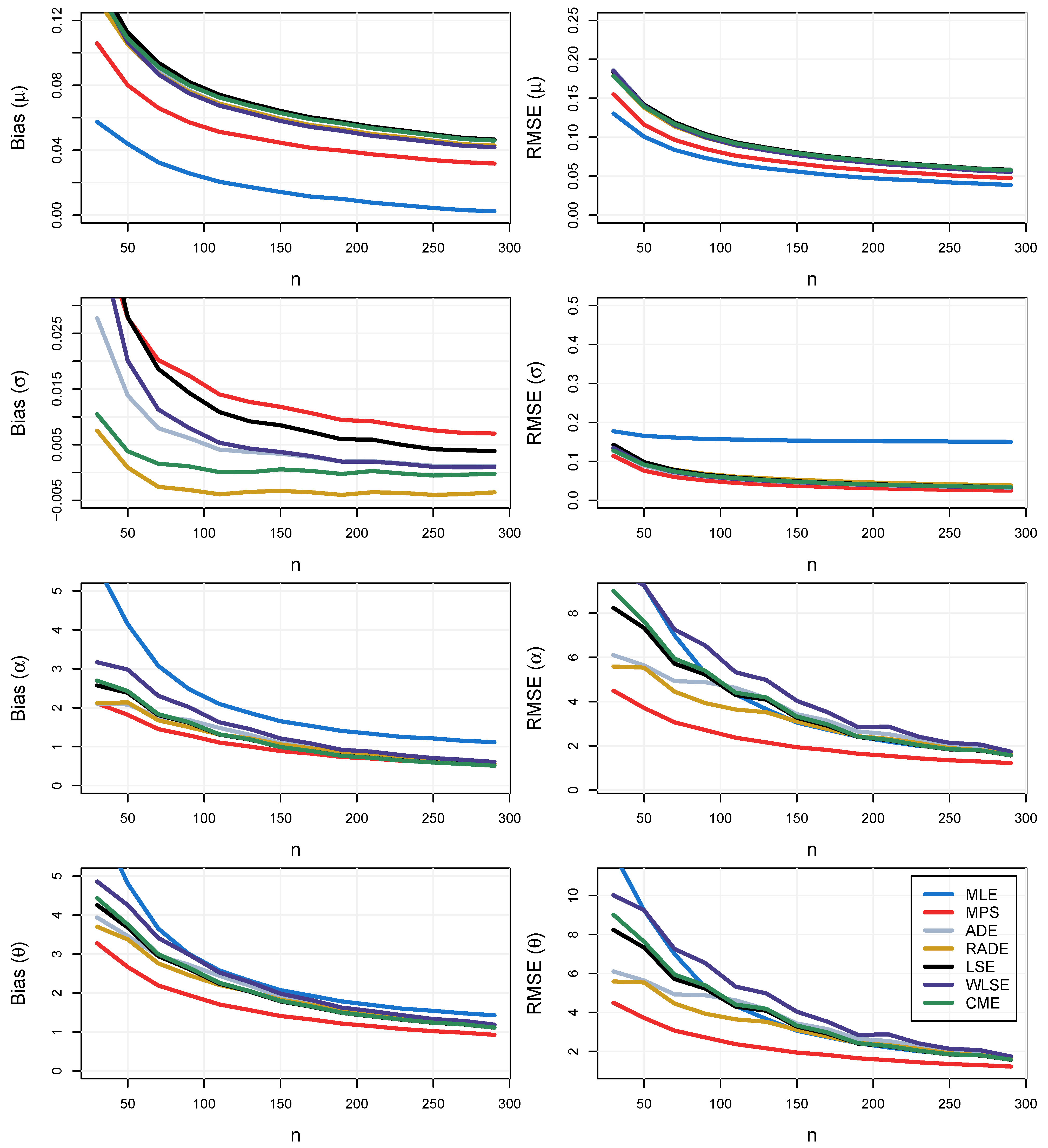
Figure 3 and Figure 4 present the performance of the estimators in terms of the bias and MSE for the parameters , , and when using the MLE, LSQ, WLQ, MPS, CME, ADE, and RADE with simulated samples and different values of n. It can be observed that the MLE did not return adequate estimates for some parameter values and only converged for samples of large sizes (moreover, an identifiability problem was noticeable when the MLE was adopted). These results show a drawback in the current approaches to obtaining parameter estimates with an ASN distribution. Although there is not a method that uniformly returns better estimates for all parameters and different parameter values, we observed that the MPS obtained the best results in terms of the minimum bias and MSE. Additionally, obtaining an estimate for was quite challenging, but the MPS returned the smallest bias for this parameter. Therefore, we recommend using the MPS to obtain estimates for all practical purposes.
5. Results
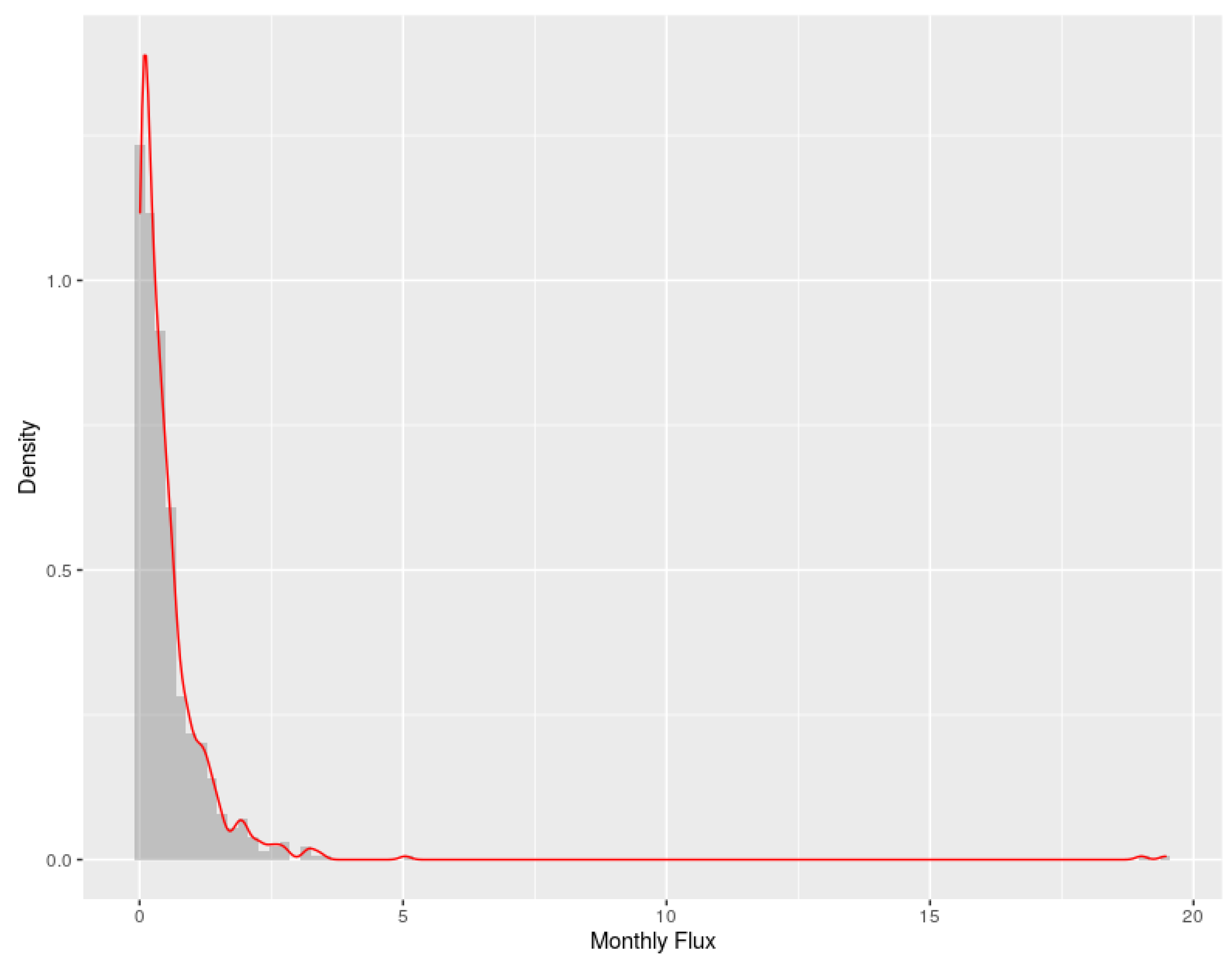
As we stated in Section 2, the motivation of this paper was driven by the water flux in the Atacama Desert or, more precisely, in the surroundings of Copiapó city. Figure 5 shows the empirical density of this phenomenon; a high concentration of low values is presented (near zero), although important events were also captured in this 10-year time window, such as a large amount of rainfall that caused a large leptokurtosis.
Table 2 presents the statistical summaries (minimum, first quartile, median, mean, third quartile, and maximum) of the water flux by month. Because the weather is very constant in the region, the seasonality across years can be ignored, as low flux is common (close values through the minimum of the months). Nonetheless, the cycle in each month is essential; given events such as defrosting at the end of spring/beginning of summer (higher values in the third quartile in November and December), it is expected to that more water will be received in the system.
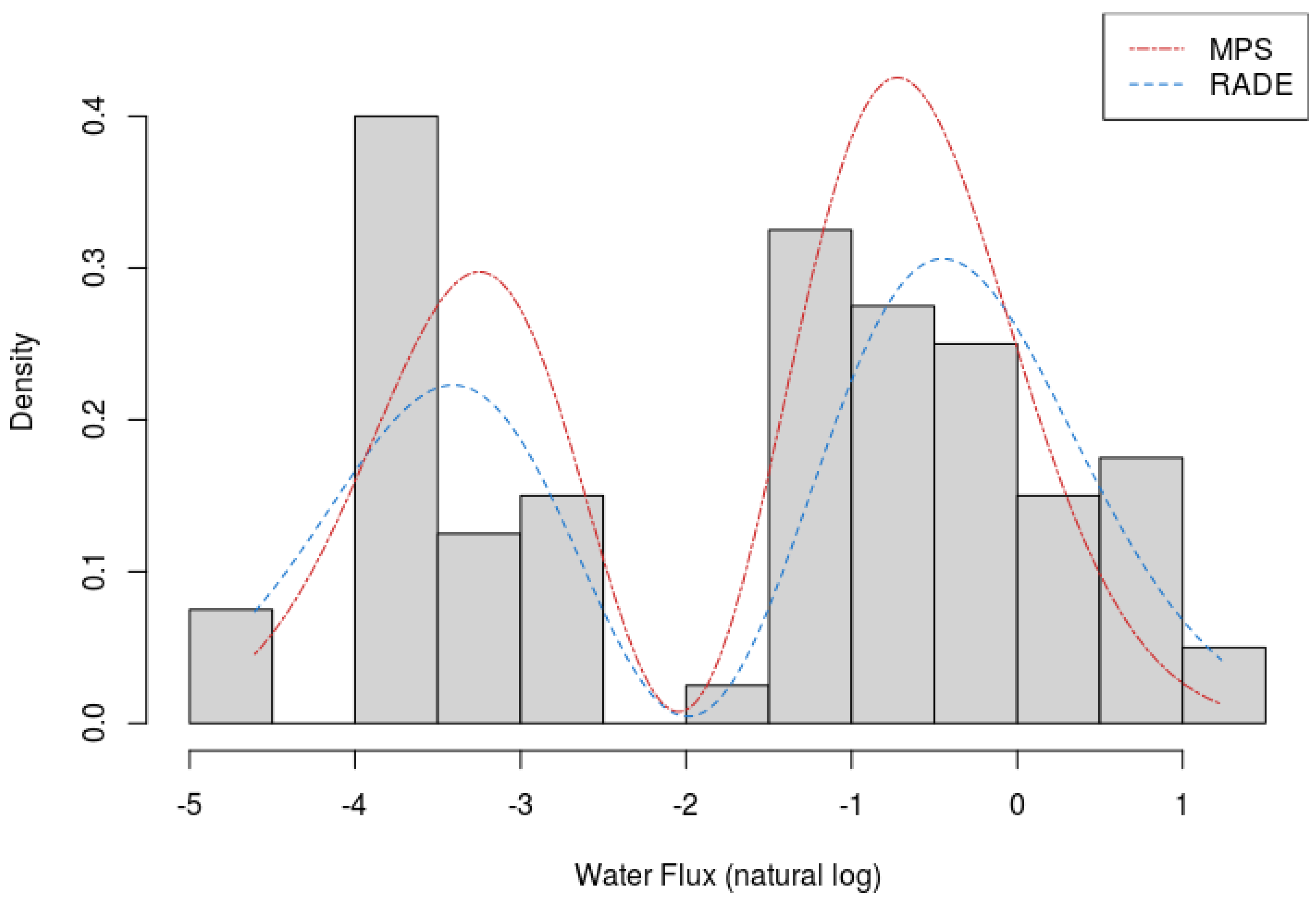
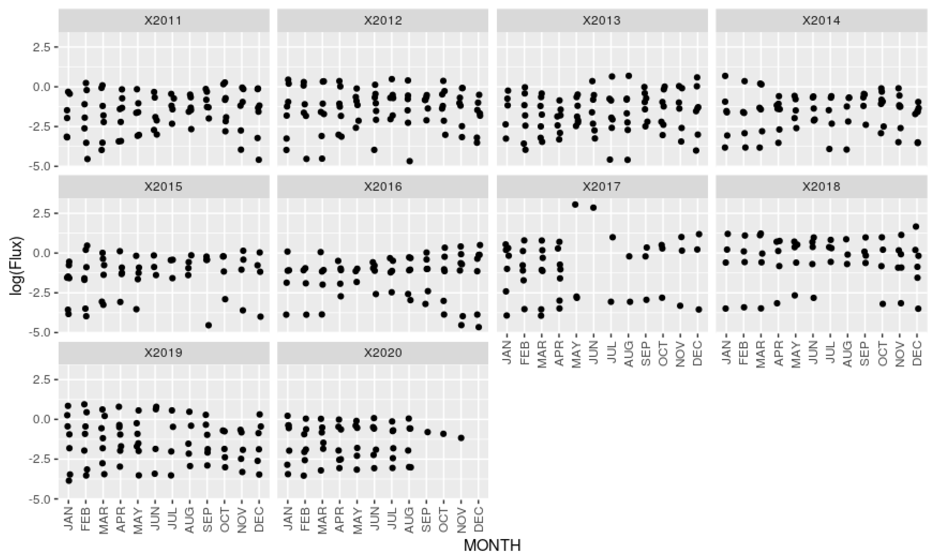
Logarithmic transformations have been used for a long time [36], though a normal distribution is often obtained. In some other situations, this is not the case; for instance, the dynamic of the water flux in the observed period, which is shown in Figure 6, shows the presence of bimodality in this data transformation, and its monthly representation is shown in Figure 7. It is essential to mention that the maximum historical values were in May and June (of 2017); they were related to the heavy rains that occurred in the region, which are also notable in the previous Table 2.
The empirical distribution of this phenomenon is visualized in Figure 6, in which the dashed lines represents the adjusted density functions: the MPS in red and the RADE in blue. The initial values used to start the iteration procedures were obtained from
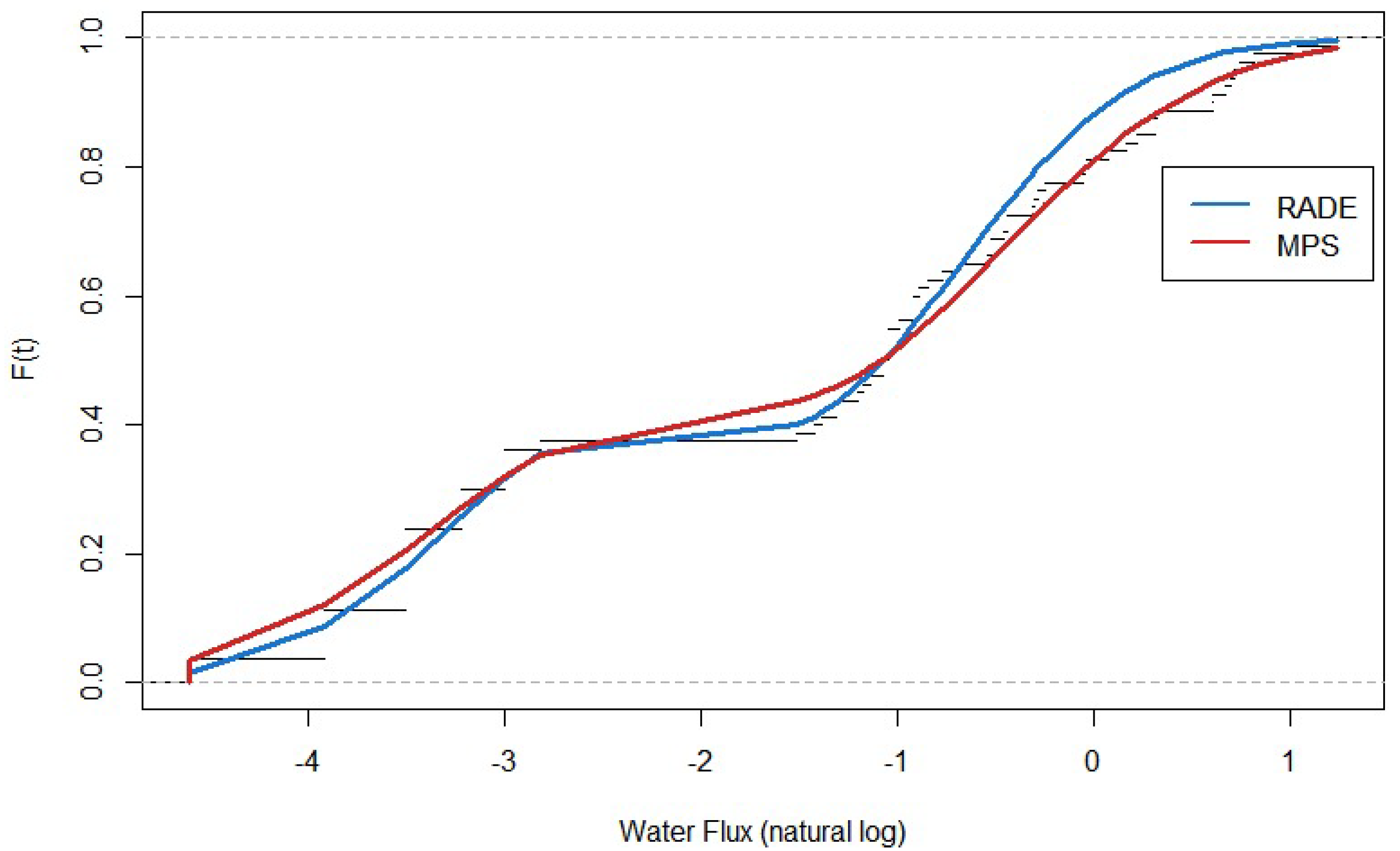
while was obtained from a grid search in the range . To confirm that the MPS returned better estimates than the others, we used Ecdf-based goodness-of-fit tests of the ASN distribution model. Figure 8 shows a particular type of distance between the functions and the observed values.
After transforming the parameters with the exponential function, the practical implications of the obtained results are that, on average, it is expected that a monthly water flux of 0.1452 (from the MPS)—compared to 0.1541 (from the RADE)—will be observed, which will show a monthly dispersion of 2.45 (MPS) versus 2.85 (RADE) by considering the value of . Regarding the asymmetry estimated with both methods (), they showed that it is expected that a frequent occurrence will be seen on the right side of the empirical distribution, that is, the recurrence of values greater than the average () is expected. Based on the results found by Elal-Olivero [18], if an ASN distribution presents a parameter , a bimodality will be obtained; if not, then shall only see a skewness. Through the transformation of the estimations towards the skewed parameter (), it bimodality was obtained (in cases of both MPS and RADE); on the other hand, through the exponentiation of , elements in the direction of skewed information were obtained. Figure 5 shows the presence of skewed data.
After confirming the ASN distribution’s goodness of fit, the occurrence of an event could be associated with its density (or cumulative) probability function. For instance, extreme values can be seen; Table 3 shows some exemplifications that consider 1%, 10%, 50%, 99%, and 99.99%.
6. Conclusions
Uncertainty reveals a wide variety of processes and experiences that may follow different rules. However, other attributions of uncertainty, such as external (disposition) versus internal factors (ignorance), are assessed through statistical inference with certain philosophical interpretations of probability [37]. The utilities of each possible outcome lead to the choice of rational actions regardless of the observed results’ uncertainty.
The example presented by this paper is the modeling of water flux, which is an essential element that has been placed under stress by significant population growth and an increase in the demand for water supply (for agriculture, industrial processes, mineral extraction, and human consumption) [38]. Therefore, planning the logistics of excessive water decisions according to their probabilistic distributions helps in unraveling this complex task [39,40]; this can be initiated by the analysis of the water flux, especially when environmental factors present limited sources for the water levels.
In the Atacama Desert, a north–south geographic band that is mainly located in northern Chile, precipitation is only a few millimeters per year, making it one of the driest places on Earth [41,42]. However, the vast expanses of the desert are punctuated by fertile valleys with rivers that originate in the central Andes and flow into the Pacific Ocean. Along these rivers, human populations have logically settled, exploiting this rare and precious water more and more throughout history, especially with the growing development of the mining industry, which is logically interested in the mineral resources of the Cordillera.
The hydrological regime of these rivers is characteristic of arid areas: Water flows from the peaks after the melting of the snowfall, glaciers, and permafrost located in the upper parts of the Cordillera [43]. In the context of climate change, it is therefore essential to understand the global hydrological cycles of these regions in order to set up a sustainable management policy [44]. This requires the implementation of tools for forecasting river flows, relative humidity, or any other water-related quantities, resulting in an inevitable need for in-depth knowledge of the physical phenomena that govern the entire hydrological cycle and, more precisely, the complex interactions among climate, ice, snow, and river flows.
Thus, this work proposed the investigation of different inference methods for the ASN probabilistic distribution, which is a promising and flexible distribution. Bimodality was noticeable and skewed information was observed in the historical series, but the distribution was nevertheless accommodated by the adopted probabilistic approach.
By using real-time analysis, big data solutions can now be implemented, as the process’s probabilistic function was estimated and evidence of the goodness of fit was shown. In addition to the elements of the ASN distribution shown here, monitoring charts and other statistical process control (SPC) tools can also be explored because parametric distributions are often adopted. Future work should expand on the reasoning of the quantile estimations with explainable features (in a regression structure) that are associated with this problem, and forecasting may also be a motivation for future research.
Author Contributions
Conceptualization, methodology, software, writing—original draft preparation, D.C.d.N. and P.L.R.; validation, D.E.-O. and M.C.-A.; writing—review and editing, F.L., D.E.-O., and M.C.-A.; supervision and project administration, F.L. and D.E.-O.; funding acquisition, D.E.-O. and M.C.-A. All authors have read and agreed to the published version of the manuscript.
Funding
Diego Nascimento acknowledges the support from the São Paulo State Research Foundation (FAPESP process 2020/09174-5). Pedro L. Ramos acknowledges the support from the São Paulo State Research Foundation (FAPESP process 2017/25971-0). Francisco Louzada acknowledges the support from the São Paulo State Research Foundation (FAPESP Processes 2013/07375-0) and CNPq (grant no. 301976/2017-1).
Institutional Review Board Statement
Not applicable.
Informed Consent Statement
Not applicable.
Data Availability Statement
The data that support the findings of this study are available in Direccion General de Aguas at https://snia.mop.gob.cl/BNAConsultas/ (accessed on 4 May 2021). These data were derived from resources available in the public domain.
Conflicts of Interest
The authors declare no conflict of interest.
References
- Cox, D.; Kartsonaki, C.; Keogh, R.H. Big data: Some statistical issues. Stat. Probab. Lett. 2018, 136, 111–115. [Google Scholar] [CrossRef]
- Efron, B.; Hastie, T. Computer Age Statistical Inference; Cambridge University Press: Cambridge, UK, 2016; Volume 5. [Google Scholar]
- Smith, J.Q. Decision Analysis: A Bayesian Approach; Chapman & Hall, Ltd.: London, UK, 1987. [Google Scholar]
- Leonelli, M.; Riccomagno, E.; Smith, J.Q. Coherent combination of probabilistic outputs for group decision making: An algebraic approach. OR Spectr. 2020, 42, 499–528. [Google Scholar] [CrossRef]
- Swain, J.J.; Venkatraman, S.; Wilson, J.R. Least-squares estimation of distribution functions in johnson’s translation system. J. Stat. Comput. Simul. 1988, 29, 271–297. [Google Scholar] [CrossRef]
- Cheng, R.; Amin, N. Maximum product of spacings estimation with application to the lognormal distribution. Math. Rep. 1979, 79, 1. [Google Scholar]
- Ranneby, B. The maximum spacing method. an estimation method related to the maximum likelihood method. Scand. J. Stat. 1984, 11, 93–112. [Google Scholar]
- Luceño, A. Fitting the generalized pareto distribution to data using maximum goodness-of-fit estimators. Comput. Stat. Data Anal. 2006, 51, 904–917. [Google Scholar] [CrossRef]
- Louzada, F.; Ramos, P.L.; Ferreira, P.H. Exponential-poisson distribution: Estimation and applications to rainfall and aircraft data with zero occurrence. Commun. Stat. Simul. Comput. 2020, 49, 1024–1043. [Google Scholar] [CrossRef]
- Ramos, P.L.; Nascimento, D.C.; Ferreira, P.H.; Weber, K.T.; Santos, T.E.; Louzada, F. Modeling traumatic brain injury lifetime data: Improved estimators for the generalized gamma distribution under small samples. PLoS ONE 2019, 14, e0221332. [Google Scholar] [CrossRef] [Green Version]
- Bonnail, E.; Lima, R.C.; Turrieta, G.M. Trapping fresh sea breeze in desert? Health status of camanchaca, atacama’s fog. Environ. Sci. Pollut. Res. 2018, 25, 18204–18212. [Google Scholar] [CrossRef]
- Du, H.; Alexander, L.V.; Donat, M.G.; Lippmann, T.; Srivastava, A.; Salinger, J.; Kruger, A.; Choi, G.; He, H.S.; Fujibe, F.; et al. Precipitation from persistent extremes is increasing in most regions and globally. Geophys. Res. Lett. 2019, 46, 6041–6049. [Google Scholar] [CrossRef] [Green Version]
- Lopes, H.F.; Salazar, E.; Gamerman, D. Spatial dynamic factor analysis. Bayesian Anal. 2008, 3, 759–792. [Google Scholar] [CrossRef]
- Mutti, P.R.; Lúcio, P.S.; Dubreuil, V.; Bezerra, B.G. Ndvi time series stochastic models for the forecast of vegetation dynamics over desertification hotspots. Int. J. Remote Sens. 2020, 41, 2759–2788. [Google Scholar] [CrossRef]
- Dutfoy, A.; Parey, S.; Roche, N. Multivariate extreme value theory-a tutorial with applications to hydrology and meteorology. Depend. Model. 2014, 2. [Google Scholar] [CrossRef] [Green Version]
- Ramos, P.; Louzada, F. The generalized weighted lindley distribution: Properties, estimation and applications. Cogent Math. 2016, 3, 1256022. [Google Scholar] [CrossRef]
- Rodrigues, G.C.; Louzada, F.; Ramos, P.L. Poisson—Exponential distribution: Different methods of estimation. J. Appl. Stat. 2018, 45, 128–144. [Google Scholar] [CrossRef]
- Elal-Olivero, D. Alpha-skew-normal distribution. Proyecciones 2010, 29, 224–240. [Google Scholar] [CrossRef] [Green Version]
- Tarnopolski, M. Analysis of gamma-ray burst duration distribution using mixtures of skewed distributions. Mon. Not. R. Astron. Soc. 2016, 458, 2024–2031. [Google Scholar] [CrossRef] [Green Version]
- Yang, K.; Aziz, M. Modeling Wind Speed Distributions Using Skewed Probability Functions: A Monte Carlo Simulation with Applications to Real Wind Speed Data. Available online: https://minds.wisconsin.edu/handle/1793/79304 (accessed on 4 May 2021).
- Ara, A.; Louzada, F. The multivariate alpha skew gaussian distribution. Bull. Braz. Math. Soc. New Ser. 2019, 50, 823–843. [Google Scholar] [CrossRef]
- Dey, S.; Kumar, D.; Ramos, P.L.; Louzada, F. Exponentiated chen distribution: Properties and estimation. Commun. Stat. Simul. Comput. 2017, 46, 8118–8139. [Google Scholar] [CrossRef]
- Ramos, P.L.; Louzada, F.; Shimizu, T.K.; Luiz, A.O. The inverse weighted lindley distribution: Properties, estimation and an application on a failure time data. Commun. Stat. Theory Methods 2018, 99, 1–20. [Google Scholar] [CrossRef]
- Teimouri, M.; Hoseini, S.M.; Nadarajah, S. Comparison of estimation methods for the Weibull distribution. Statistics 2013, 47, 93–109. [Google Scholar] [CrossRef]
- Fisher, R.A. On the mathematical foundations of theoretical statistics. Philos. Trans. R. Soc. Lond. Ser. Contain. Pap. Math. Phys. Character 1922, 222, 309–368. [Google Scholar]
- Macdonald, P. An estimation procedure for mixtures of distribution. J. R. Stat. Soc. Ser. B 1971, 33, 326–329. [Google Scholar]
- Boos, D.D. Minimum anderson-darling estimation. Commun. Stat. Theory Methods 1982, 11, 2747–2774. [Google Scholar] [CrossRef]
- Stigler, S.M. The epic story of maximum likelihood. Stat. Sci. 2007, 22, 598–620. [Google Scholar] [CrossRef]
- Wolfowitz, J. The minimum distance method. Ann. Math. Stat. 1957, 28, 75–88. [Google Scholar] [CrossRef]
- Cheng, R.; Amin, N. Estimating parameters in continuous univariate distributions with a shifted origin. J. R. Stat. Soc. Ser. B 1983, 45, 394–403. [Google Scholar] [CrossRef]
- Cramér, H. On the composition of elementary errors: First paper: Mathematical deductions. Scand. Actuar. J. 1928, 1928, 13–74. [Google Scholar] [CrossRef]
- Von Mises, R. Statistik und Wahrheit; Julius Springer: Berlin/Heidelberg, Germany, 1928; Volume 20. [Google Scholar]
- Ye, Y.; Lu, G.; Li, Y.; Jin, M. Unilateral right-tail anderson-darling test based spectrum sensing for cognitive radio. Electron. Lett. 2017, 53, 1256–1258. [Google Scholar] [CrossRef]
- R Core Team. R: A Language and Environment for Statistical Computing. (Version 3.3.1); R Foundation for Statistical Computing: Vienna, Austria, 2014. [Google Scholar]
- Henningsen, A.; Toomet, O. Maxlik: A package for maximum likelihood estimation in r. Comput. Stat. 2011, 26, 443–458. [Google Scholar] [CrossRef]
- Finney, D. On the distribution of a variate whose logarithm is normally distributed. Suppl. J. R. Stat. Soc. 1941, 7, 155–161. [Google Scholar] [CrossRef]
- Kahneman, D.; Tversky, A. Variants of uncertainty. Cognition 1982, 11, 143–157. [Google Scholar] [CrossRef]
- Södergren, K.; Palm, J. How organization models impact the governing of industrial symbiosis in public wastewater management. an explorative study in sweden. Water 2021, 13, 824. [Google Scholar] [CrossRef]
- Jain, A.; Ormsbee, L.E. Short-term water demand forecast modeling techniques—Conventional methods versus ai. J. Am. Water Work. Assoc. 2002, 94, 64–72. [Google Scholar] [CrossRef]
- Tu, Z.; Gao, X.; Xu, J.; Sun, W.; Sun, Y.; Su, D. A novel method for regional short-term forecasting of water level. Water 2021, 13, 820. [Google Scholar] [CrossRef]
- Bull, A.T.; Andrews, B.A.; Dorador, C.; Goodfellow, M. Introducing the Atacama Desert; Springer: Berlin/Heidelberg, Germany, 2018. [Google Scholar]
- Grosjean, M.; Veit, H. Water Resources in the Arid Mountains of the Atacama Desert (Northern Chile): Past Climate Changes and Modern Conflicts; Springer: Dordrecht, The Netherlands, 2005. [Google Scholar]
- Donoso, G.; Lictevout, E.; Rinaudo, J.-D. Groundwater management lessons from Chile. In Sustainable Groundwater Management; Springer: Berlin/Heidelberg, Germany, 2020. [Google Scholar]
- Suárez, F.; Muñoz, J.; Fernández, B.; Dorsaz, J.-M.; Hunter, C.K.; Karavitis, C.A.; Gironás, J. Integrated water resource management and energy requirements for water supply in the Copiapó river basin, Chile. Water 2020, 6, 2590. [Google Scholar] [CrossRef] [Green Version]
Figure 1.
Visual summary of the role of probabilistic reasoning in knowledge discovery in databases as a cornerstone for the quantification of uncertainty. Statistical inference procedures enable us to draw conclusions based on a sample and generalize them to an entire population.
Figure 1.
Visual summary of the role of probabilistic reasoning in knowledge discovery in databases as a cornerstone for the quantification of uncertainty. Statistical inference procedures enable us to draw conclusions based on a sample and generalize them to an entire population.

Figure 2.
The PDF of the ASN distribution, where t is a random variable, assuming (location), (scale), and different values for (skewness).
Figure 2.
The PDF of the ASN distribution, where t is a random variable, assuming (location), (scale), and different values for (skewness).

Figure 3.
Bias and MSE of the estimates of , , and for N = 10,000 simulated samples of size n using the following methods: MLE, MPS, ADE, RADE, LSE, WLSE, and CME. Based on Figure 2, by choosing the configuration of these parameters (, , and ), a bimodal PDF can be seen, which presents a larger peak to the left and a smaller peak to the right.

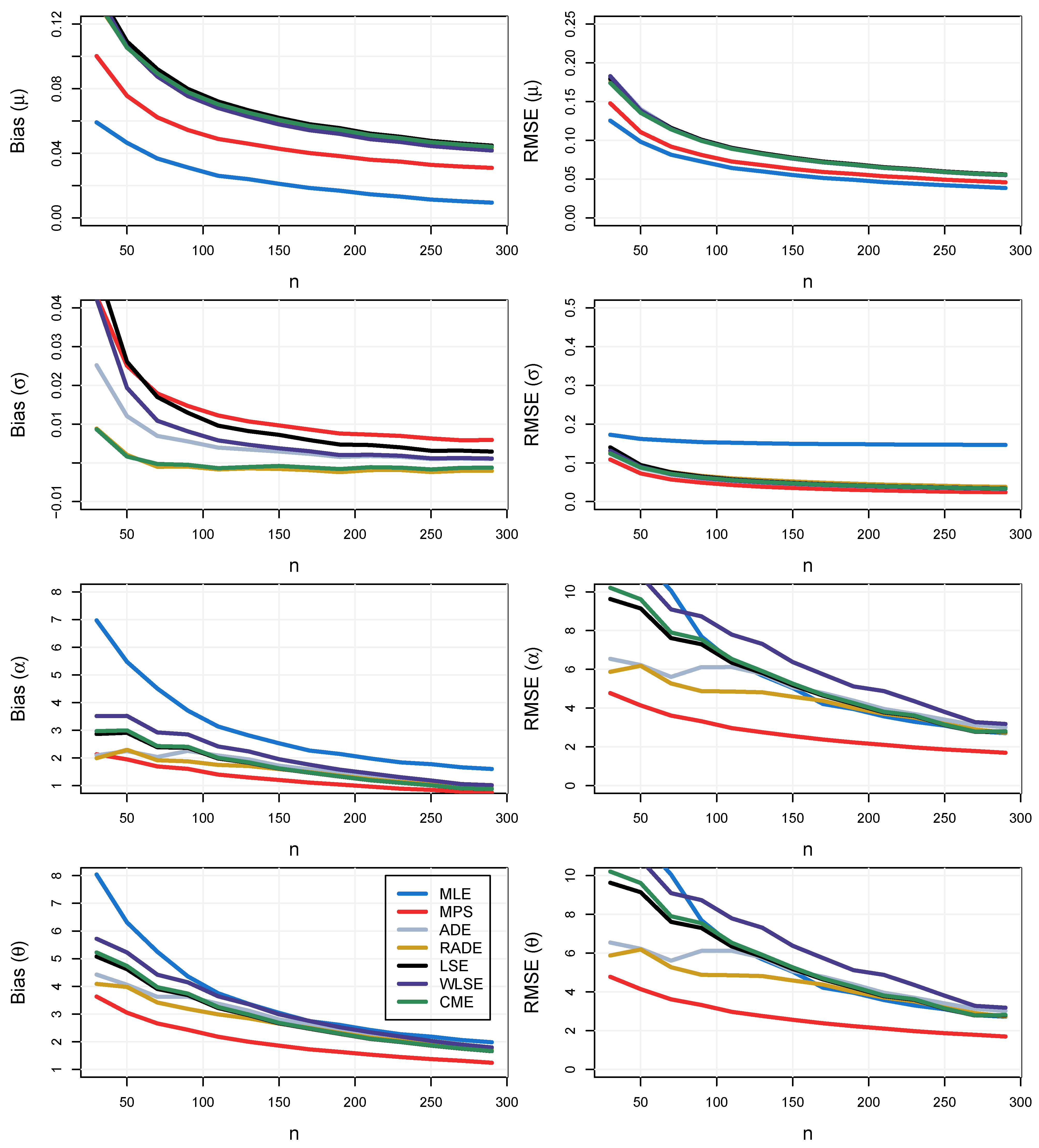
Figure 4.
Bias and MSE of the estimates of , , and for N = 10,000 simulated samples of size n using the following methods: MLE, MPS, ADE, RADE, LSE, WLSE, and CME.
Figure 4.
Bias and MSE of the estimates of , , and for N = 10,000 simulated samples of size n using the following methods: MLE, MPS, ADE, RADE, LSE, WLSE, and CME.

Figure 5.
Empirical density function of the water flux in the 21 rivers/channels in the surroundings of Copiapó city. The solid gray shade represents the density (frequency) of each of the numerical records of the water flux, and the solid red line represents a smooth adjusted function.
Figure 5.
Empirical density function of the water flux in the 21 rivers/channels in the surroundings of Copiapó city. The solid gray shade represents the density (frequency) of each of the numerical records of the water flux, and the solid red line represents a smooth adjusted function.

Figure 6.
The empirical distribution of the log of the water flux and its frequency, which is represented by gray blocks. The black dashed line represents the adjusted ASN distribution based on the MPS (), which is represented by the blue dashed line, and the RADE (), which is represented by the red dot-dashed line.

Figure 7.
The logarithm of the water flux dispersion records (y-coordinates) for each year (per panel) by month (x-coordinates).
Figure 7.
The logarithm of the water flux dispersion records (y-coordinates) for each year (per panel) by month (x-coordinates).

Figure 8.
Ecdf-based test of the ASN distribution; RADE returned an AIC estimation of 274 and MPS returned an AIC estimation of 251.
Figure 8.
Ecdf-based test of the ASN distribution; RADE returned an AIC estimation of 274 and MPS returned an AIC estimation of 251.


Table 1.
A summary of seven inferential estimation methods.
| Estimation Method | Abbreviation | Created by |
|---|---|---|
| Maximum Likelihood Estimation | MLE | Fisher [25] |
| Ordinary Least-Square Estimate | LSQ | Swain et al. [5] |
| Weighted Least-Square Estimate | WLQ | Swain et al. [5] |
| Maximum Product of Spacings | MPS | Cheng & Amin [6] |
| Cramer–von Mises Estimators | CME | Macdonald [26] |
| Anderson–Darling Estimator | ADE | Boos [27] |
| Right-Tail Anderson–Darling Estimator | RADE | Luceno [8] |
Table 2.
Summary statistics of the water flux by month.
| Month | Min. | 1st Qu. | Median | Mean | 3rd Qu. | Max. | NA’s |
|---|---|---|---|---|---|---|---|
| JAN | 0.02 | 0.06 | 0.31 | 0.5374 | 0.68 | 3.45 | 39 |
| FEB | 0.01 | 0.065 | 0.2 | 0.5165 | 0.6875 | 3.15 | 40 |
| MAR | 0.01 | 0.06 | 0.31 | 0.5449 | 0.85 | 3.24 | 37 |
| APR | 0.03 | 0.08 | 0.27 | 0.4494 | 0.5275 | 2.25 | 36 |
| MAY | 0.03 | 0.12 | 0.29 | 0.7859 | 0.55 | 19.47 | 47 |
| JUN | 0.02 | 0.12 | 0.35 | 0.9106 | 0.62 | 19.01 | 51 |
| JUL | 0.01 | 0.14 | 0.46 | 0.5636 | 0.64 | 2.58 | 53 |
| AUG | 0.01 | 0.1125 | 0.33 | 0.4692 | 0.6175 | 2.23 | 50 |
| SEP | 0.01 | 0.2025 | 0.45 | 0.5356 | 0.6775 | 2.66 | 52 |
| OCT | 0.02 | 0.1 | 0.37 | 0.5229 | 0.77 | 2.46 | 49 |
| NOV | 0.01 | 0.0775 | 0.365 | 0.5536 | 0.855 | 3.36 | 48 |
| DEC | 0.01 | 0.055 | 0.265 | 0.5639 | 0.7975 | 5.04 | 46 |
Table 3.
Cumulative event probability based on the adjusted ASN distribution (using RADE).
| CUM Prob. | 1% | 10% | 50% | 99% | 99.99% |
| Flux | 0.0059 | 0.0174 | 0.3396 | 1.5068 | 16.281 |
Publisher’s Note: MDPI stays neutral with regard to jurisdictional claims in published maps and institutional affiliations. |
© 2021 by the authors. Licensee MDPI, Basel, Switzerland. This article is an open access article distributed under the terms and conditions of the Creative Commons Attribution (CC BY) license (https://creativecommons.org/licenses/by/4.0/).
Share and Cite
MDPI and ACS Style
Nascimento, D.C.d.; Ramos, P.L.; Elal-Olivero, D.; Cortes-Araya, M.; Louzada, F. Generalizing Normality: Different Estimation Methods for Skewed Information. Symmetry 2021, 13, 1067. https://doi.org/10.3390/sym13061067
AMA Style
Nascimento DCd, Ramos PL, Elal-Olivero D, Cortes-Araya M, Louzada F. Generalizing Normality: Different Estimation Methods for Skewed Information. Symmetry. 2021; 13(6):1067. https://doi.org/10.3390/sym13061067
Chicago/Turabian StyleNascimento, Diego Carvalho do, Pedro Luiz Ramos, David Elal-Olivero, Milton Cortes-Araya, and Francisco Louzada. 2021. "Generalizing Normality: Different Estimation Methods for Skewed Information" Symmetry 13, no. 6: 1067. https://doi.org/10.3390/sym13061067
Note that from the first issue of 2016, this journal uses article numbers instead of page numbers. See further details here.