
An Asymmetric Bimodal Double Regression Model


1
Departamento de Matemática, Facultad de Ingeniería, Universidad de Atacama, Copiapó 1530000, Chile
2
Departamento de Ciencias Matemáticas y Físicas, Facultad de Ingeniería, Universidad Católica de Temuco, Temuco 4780000, Chile
3
Department of Statistics, Institute of Exact Sciences, Federal University of Juiz de Fora, Juiz de Fora 36036-900, MG, Brazil
*
Author to whom correspondence should be addressed.
Symmetry 2021, 13(12), 2279; https://doi.org/10.3390/sym13122279
Submission received: 26 October 2021
/
Revised: 24 November 2021
/
Accepted: 26 November 2021
/
Published: 30 November 2021
(This article belongs to the Special Issue Symmetric and Asymmetric Bimodal Distributions with Applications)
Abstract
:In this paper, we introduce an extension of the sinh Cauchy distribution including a double regression model for both the quantile and scale parameters. This model can assume different shapes: unimodal or bimodal, symmetric or asymmetric. We discuss some properties of the model and perform a simulation study in order to assess the performance of the maximum likelihood estimators in finite samples. A real data application is also presented.
1. Introduction
A wide range of phenomena can be defined more appropriately using probability distributions. This description is very useful because of the properties associated with a distribution: expectation, shape, range, etc. However, fitting data can be difficult when their distribution is bimodal, which occurs commonly in practice: in astrophysics, the metallicity of the globular cluster system in the Milky Way (see [1]); in ecology, the tree cover of moist savanna and tropical forest ecosystems (see [2]); in genetics, gene expression measurements (see [3]). Other practical examples of bimodality in data can be seen in [4,5,6]. In the literature, there are many proposals discussing bimodal distributions; e.g., the works of [7,8,9,10,11,12]. Bimodal data can be fitted by a mixture of two unimodal distributions. When the mixture is created from the same model, the main difficulty is the non-identifiability of the proposed mixture model. The traditional example is the mixture of normals. Alternatively, the most workable practical method is to use a distribution which already has bimodal properties. For the latter situation, we introduce the gamma–sinh Cauchy (GSC) distribution, proposed by [13]. We note that the initials GSC can be found in the literature as an acronym for Generalized Skew-Cauchy, and readers should be aware of this when reviewing the literature. This model has uni/bimodal properties. However, unlike the distributions discussed in the works mentioned above, in this model, one of the parameters can be interpreted as the q-th quantile under certain conditions. This is very convenient, because it allows covariates to be introduced into non-homogeneous populations directly. The probability density function (pdf) for the GSC distribution is given by
where , , and . The corresponding cumulative distribution function (cdf) is given by
where denotes the cdf of the gamma distribution with shape and scale parameters equal to and 1 respectively. The GSC can be asymmetric or symmetric and, as the main advantage, its cdf has a closed-form expression which can be generated quickly in many different softwares. This is useful for generating random data, besides defining quantiles.
Regression models seek to describe the behavior of a variable of interest (or response) from covariables (explanatory variables). In general, a function called a link function links a characteristic of the response variable to the explanatory variables through parameters estimated from observed data. In our case, the response variable is bimodal and described by the GSC distribution, while the relationship between the response and explanatory variables is through the quantile. This type of relation is known as quantile regression. The literature on parametric models in the context of quantile regressions has increased considerably in recent years. For instance, for responses in the unit interval, see the works of [14,15]; for responses in the positive line see the work of [16]; and for responses in the real line see the works of [17,18].
The main advantage of quantile regression is that it is more robust against outliers. The advantage is that we can have a more informative approach to the response than simply modeling some specific measure of the population, such as the mean or median. The applicability of this method can be seen in ecology [19], econometrics [20], environmetrics [21], and medicine [22], for instance. In general terms, the distributions are not parametrized directly in terms of a general quantile or any specific quantile, except for some particular cases. For instance, for the model, represents the mean and the median of the distribution, but the q-th quantile is given by , where is the q-th of the standard normal distribution. On the other hand, which quantile is of interest depends on the research. In some cases, small quantiles will be of interest, whereas in other contexts, large quantiles will be the focus. For instance, in a nutrition context, larger quantiles of weight are of interest because they enable the nutritionist to define which patients are at higher risk; on this basis, they can define special treatments for such patients.
In view of the importance of bimodal distributions, the chief object of this paper is to build on the quantile regression structure in the GSC distribution. Double regression has been studied quite extensively in the literature; for example, the authors of [23] consider a regression structure for both components based on a new parameterization indexed by mean and dispersion parameters; in [24], a regression model is proposed that is useful for situations where the variable of interest is continuous and restricted to the positive real line and is related to other variables through the mean and precision parameters; and in [25], a new parameterization of the gamma distribution is used that is indexed by mode and precision parameters.
The paper is organized as follows. In Section 2, we develop the GSC regression model with its properties. In Section 3, we perform a small-scale simulation and evaluate the point estimation. An application to real data, which illustrates the usefulness of the proposed model, is discussed in Section 4. Finally, conclusions are given in Section 5.
2. The GSC Regression Model
Gómez et al. [13] show that and then, for a fixed such as
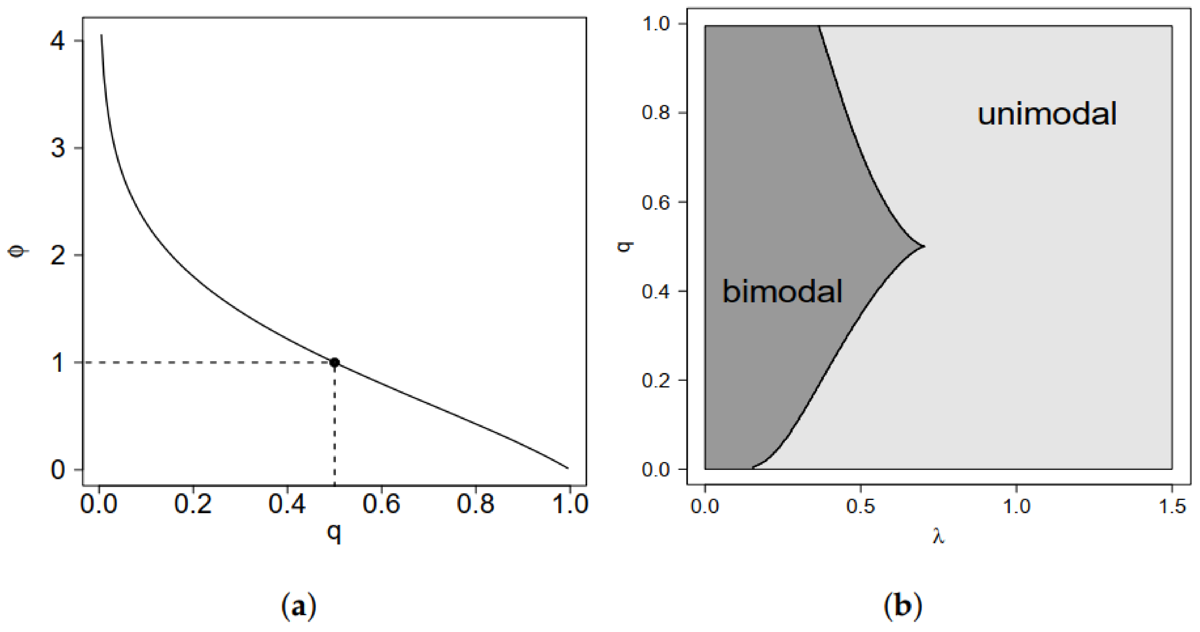
the parameter represents the q-th quantile of the distribution. This equation can be solved numerically. Henceforth, we use the notation GSC to refer to a random variable with GSC distribution where is fixed as in (1), is the q-th quantile of the distribution, is a scale parameter and is a shape parameter. Figure 1 shows the relation between q and and the regions where the model is unimodal or bimodal, depending on the modeled quantile q and the parameter . Note that, for , we have such that the model is unimodal for and bimodal for . In the next proposition, we enunciate a property related to the unimodality of the model.
Proposition 1.
The GSCmodel is unimodal forand bimodal for.
Proof.
Since and are location and scale parameters, without a loss of generality, we can consider and . Deriving the pdf of the GSC model in relation to x, we obtain that
Note that if and only if or . From the last equation, it follows that , which has two solutions if , one solution if , and no solution if . Therefore,
- For , the equation has three solutions. In this case, , and , . Then, are the two modes of the distribution.
- For , the equation has one solution. In this case, , and , . Then, is the only mode of the distribution.
□
Suppose now that we are interested in modeling the q-th quantile of the distribution for a non-homogeneous population. We assume that, for a fixed , the q-th quantile of the distribution and the scale parameter satisfy the following functional relations:
where and are vectors of unknown regression coefficients such that , with ; and and are the observations of the known regressors and . Note that the vector is linked with the parameter using the identity link; then, interpretations for the covariates in can be performed using the same idea as an ordinary linear regression. For instance, if the jth covariate is a quantitative variable, then, fixing the rest of the covariates, the q-th quantile of the distribution increases by units when is increased to . Similarly, for the regression coefficients related to the scale parameter, after fixing the rest of the covariates, the scale of the distribution for the q-th quantile of the distribution is increased by units when is increased to , . We highlight that in [13], a regression structure was assumed only for . However, the assumption that all the observations have the same scale parameter could be unrealistic, as each observation could have its own scale. For this reason, it seems reasonable to assume this double regression structure.
In this setting, the log-likelihood function for , up to a constant, is given by
where . The maximum likelihood (ML) estimator of , say , is obtained by maximizing in relation to . For this model, such a maximization procedure does not provide a closer form, meaning that numerical procedures need to be implemented. Specifically, we use the Broyden–Fletcher–Goldfarb–Shanno (BFGS) quasi-Newton method; see [26] (p. 199). This procedure is implemented in the R software [27]. The programs are available on request. Finally, under regularity conditions, satisfies that
where denotes the standard multivariate distribution and denotes the estimated Hessian matrix of the log-likelihood function in relation to .
3. Simulation Study
In this section, we present a simulation study to evaluate the performance of ML estimates in finite samples. The computational procedure is implemented using R software [27]. Values of the GSC distribution were drawn using inverse transform sampling. We considered a scheme with two covariates, both simulated from the uniform distribution between −2 and 2. We considered combinations of values for the quantile and ; vectors for and ; vectors for and ; and the parameter and . We also considered three sample sizes: 100, 200 and 500. Based on 5000 replicates, we compute the mean of the estimated bias for each estimator (bias), the mean of the estimated standard errors (SE), the root of the estimated mean squared error (RMSE), and the 95% coverage probabilities (CP). Table 1 summarizes the results. From Table 1, it can be observed that the bias, SE, and RMSE for all the parameters tend to approach zero when the sample size is increased, showing that the ML estimates obtained are asymptotically consistent. On the other hand, the CP values are closer to the nominal values used in their construction (95%), suggesting that the asymptotic distribution in Equation (3) is reasonable, even in finite samples.
4. Application
To illustrate the GSC double regression model, we consider the Australian data set available in the package sn in R [28], which includes data on 202 athletes collected at the Australian Institute of Sport. Codes were performed in [27] and are available upon request. Our main aim is to explain the body fat percentage (Bfat) in terms of the body mass index (bmi) and the lean body mass (lbm). Particularly, we consider Bfat, where satisfies (1), and for , we have that
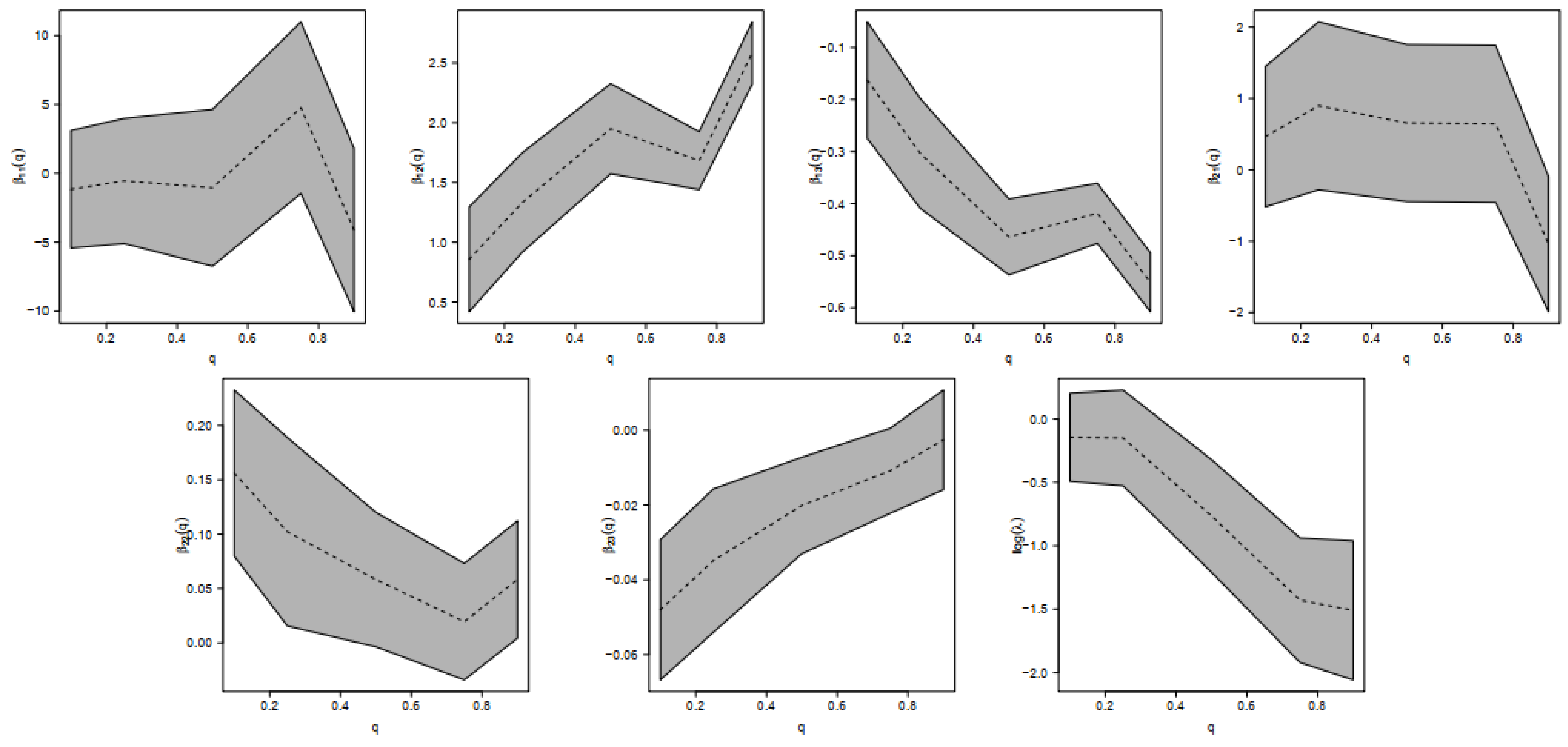
In other words, the bmi and lbm explain both the q-th quantile of Bfat and the scale of the distribution. The same structure of covariates was considered in [13], but without modeling the scale parameter; i.e., considering . We refer to those models as GSC and GSC for the cases where is modeled and not modeled, respectively. We considered . Our approach is compared with the skewed Laplace (SKL) model in [29]. Table 2 shows the Akaike information criterion (AIC [30]) for the three models. We also present the statistic for the likelihood ratio test (LRT) to test versus or , for all the quantiles considered. In addition, we also compute the quantile residuals [31] for the GSC model. If the model is correctly specified, the residual should be a random sample from the standard normal distribution. We checked this assumption with the traditional Kolmogorov–Smirnov test. Note that the GSC presents the lowest AIC for the quantiles up to the median, and GSC presents the lowest AIC for the rest of the quantiles. This is explained because, according to the LRT, the coefficients related to the bmi and lbm variables are not significant (under any common level of significance) for modeling the scale parameter for and , while they are significant for the rest of the quantiles. Finally, based on the quantile residuals, the GSC double regression model seems to be appropriate for modeling all quantiles, except the largest. Figure 2 also shows the regression coefficients in terms of the quantiles and their respective 95% confidence intervals. Note that and are significant (based on 5% significance) for all the quantiles considered; i.e., the bmi and lbm variables are relevant for explaining the different quantiles of Bfat. Specifically, we can obtain the following interpretations for and :
- (Interpreting ) For a fixed lbm, for athletes in the lowest 10% of Bfat, the Bfat is increased by 0.8572 units (95% confidence interval 0.4191; 1.2954) for each unit increase in bmi, and for athletes in the highest 90% of Bfat, the Bfat is increased by 2.5834 units (95% confidence interval 2.3227; 2.8442) for each unit increase in bmi.
- (Interpreting ) For a fixed bmi, for athletes in the lowest 10% of Bfat, the Bfat is decreased by 0.3039 units (95% confidence interval −0.4093; −0.1984) for each unit increase in lbm, and for athletes in the highest 10% of Bfat, the Bfat is decreased by 0.5511 units (95% confidence interval −0.6077; −0.4945) for each unit increase in lbm.
We highlight the large difference between the interpretations for athletes in the lowest 10% and highest 10% of Bfat.
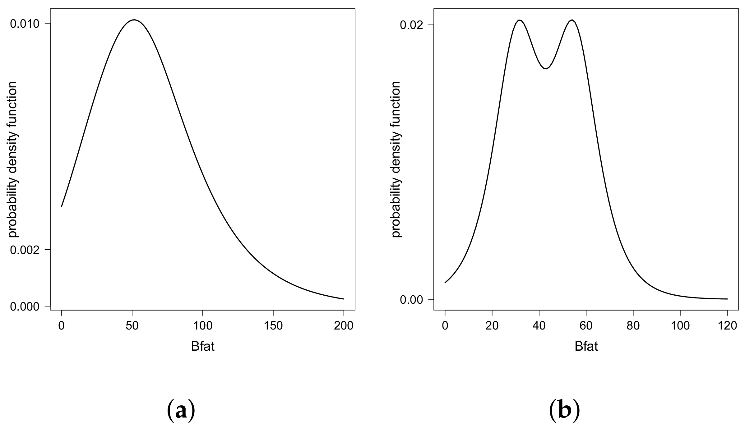
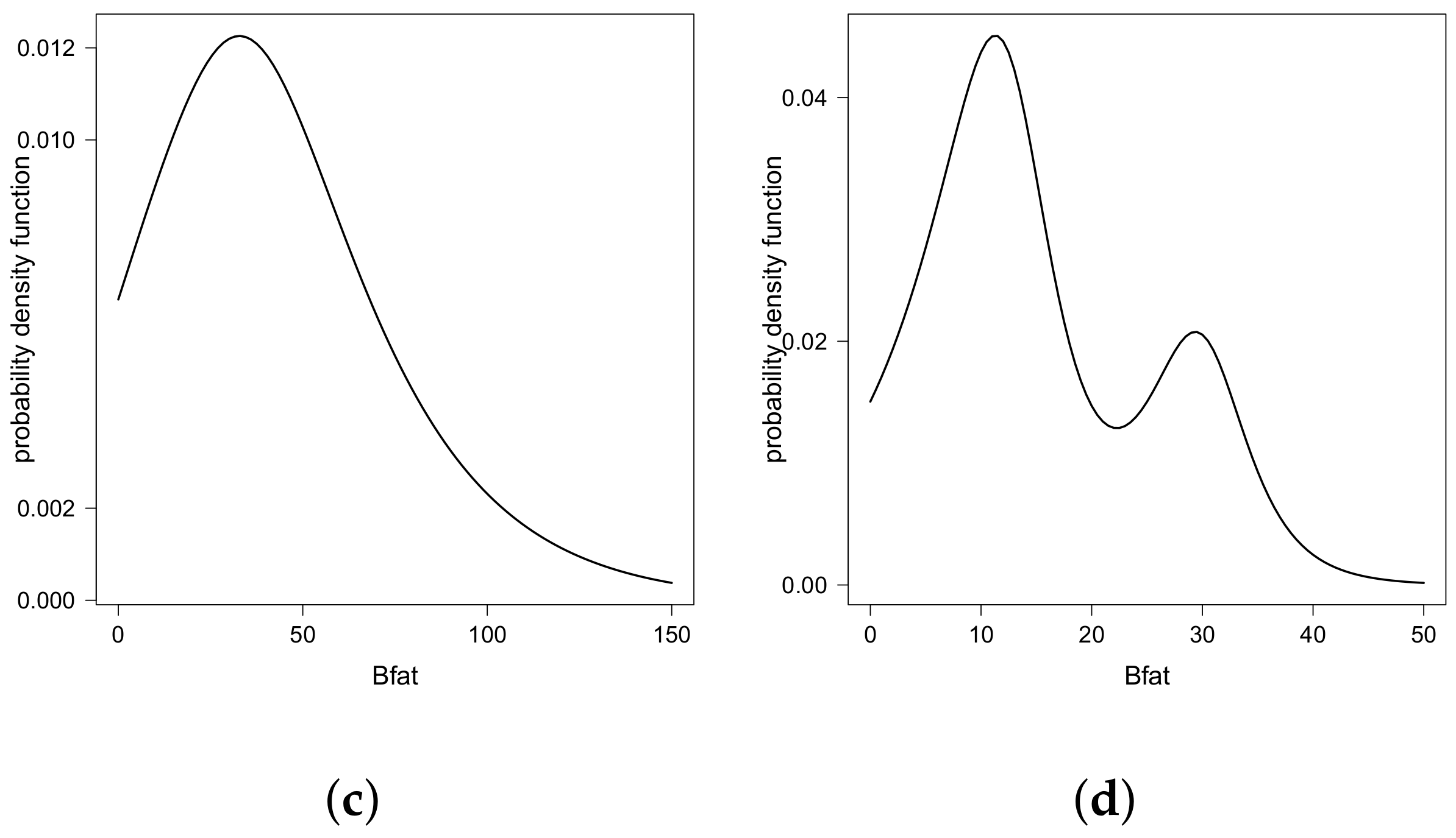
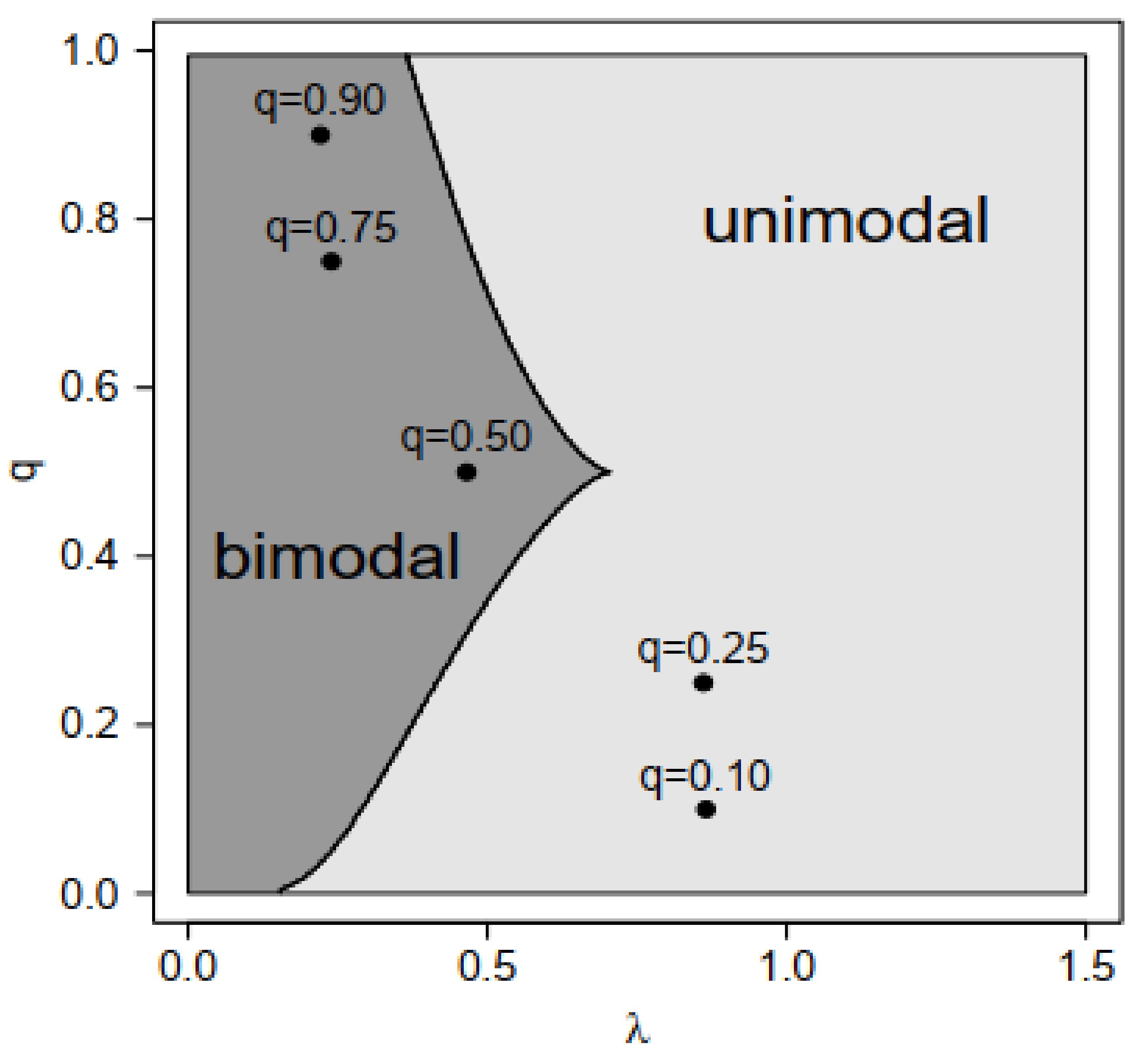
Finally, Figure 3 shows the different estimated pdf values for the Bfat under different scenarios for bmi and lbm. We note that these estimated pdf values assumed different shapes—unimodal, bimodal symmetric, and bimodal asymmetric—justifying the use of the double regression GSC model in this example. Finally, Figure 4 shows the pairs for the five quantiles modeled, identifying the unimodal and bimodal cases.
5. Conclusions
In this paper, we present a new extension of the GSC model, introducing a double regression structure to model both the quantile and the scale of the distribution. This structure produces a competitive model for modeling heterogeneous populations with different shapes: unimodal symmetric, unimodal asymmetric, bimodal symmetric, and bimodal asymmetric. The illustration with a real data set shows that the model provides better performance than other proposals in the literature. A limitation of the model is that the shape parameter is common for all the observations. Further extensions should include covariates in this parameter also.
Author Contributions
Conceptualization, Y.M.G. and D.I.G.; methodology, Y.M.G. and D.I.G.; software, Y.M.G. and D.I.G.; validation, O.V. and T.M.M.; formal analysis, Y.M.G. and D.I.G.; investigation, O.V. and T.M.M.; resources, O.V. and T.M.M.; data curation, Y.M.G. and D.I.G.; writing—original draft preparation, Y.M.G. and D.I.G.; writing—review and editing, O.V. and T.M.M. All authors have read and agreed to the published version of the manuscript.
Funding
Nothing to declare.
Institutional Review Board Statement
Not applicable.
Informed Consent Statement
Not applicable.
Data Availability Statement
For data, we refer the reader to [28].
Conflicts of Interest
The authors declare no conflict of interest.
References
- Ashman, K.M.; Bird, C.M.; Zepf, S.E. Detecting bimodality in astronomical datasets. Astron. J. 1994, 108, 2348–2361. [Google Scholar] [CrossRef] [Green Version]
- De Michele, C.; Accatino, F. Tree cover bimodality in savannas and forests emerging from the switching between two fire dynamics. PLoS ONE 2014, 9, e91195. [Google Scholar] [CrossRef] [Green Version]
- Wang, J.; Wen, S.; Symmans, W.F.; Pusztai, L.; Coombes, K.R. The bimodality index: A criterion for discovering and ranking bimodal signatures from cancer gene expression profiling data. Cancer Inform. 2009, 7, 199–216. [Google Scholar] [CrossRef] [Green Version]
- Freeman, J.B.; Dale, R. Assessing bimodality to detect the presence of a dual cognitive process. Behav. Res. Methods 2013, 45, 83–97. [Google Scholar] [CrossRef] [Green Version]
- Sambrook-Smith, G.H.; Nicholas, A.P.; Ferguson, R.I. Measuring and defining bimodal sediments: Problems and implications. Water Resour. Res. 1997, 33, 1179–1195. [Google Scholar] [CrossRef]
- Sturrock, P.A. Analysis of bimodality in histograms formed from GALLEX and GNO solar neutrino data. Sol. Phys. 2008, 249, 1–10. [Google Scholar] [CrossRef] [Green Version]
- Gómez, H.W.; Elal-Olivero, D.; Salinas, H.S.; Bolfarine, H. Bimodal extension based on the skew-normal distribution with application to pollen data. Environmetrics 2018, 22, 50–62. [Google Scholar] [CrossRef]
- Venegas, O.; Salinas, H.S.; Gallardo, D.I.; Bolfarine, H.; Gómez, H.W. Bimodality based on the generalized skew-normal distribution. J. Stat. Comput. Simul. 2018, 88, 156–181. [Google Scholar] [CrossRef]
- Butt, N.S.; Khalil, M.G. A new bimodal distribution for modeling asymmetric bimodal heavy-tail real lifetime data. Symmetry 2020, 12, 2058. [Google Scholar] [CrossRef]
- Iriarte, Y.A.; de Castro, M.; Gómez, H.W. A Unimodal/Bimodal Skew/Symmetric Distribution Generated from Lambert’s Transformation. Symmetry 2021, 13, 269. [Google Scholar] [CrossRef]
- Reyes, J.; Gómez-Déniz, E.; Gómez, H.W.; Calderín-Ojeda, E. A bimodal extension of the exponential distribution with applications in risk theory. Symmetry 2021, 13, 679. [Google Scholar] [CrossRef]
- Reyes, J.; Arrué, J.; Leiva, V.; Martín-Barreiro, C. A new Birnbaum–Saunders distribution and its mathematical features applied to bimodal real-world data from environment and medicine. Mathematics 2021, 9, 1891. [Google Scholar] [CrossRef]
- Gómez, Y.; Gómez-Déniz, E.; Venegas, O.; Gallardo, D.I.; Gómez, H.W. An asymmetric bimodal distribution with application to quantile regression. Symmetry 2019, 11, 899. [Google Scholar] [CrossRef] [Green Version]
- Bayes, C.L.; García, C. A new robust regression model for proportions. Bayesian Anal. 2012, 7, 841–866. [Google Scholar] [CrossRef]
- Bayes, C.L.; Bazán, J.L.; de Castro, M. A quantile parametric mixed regression model for bounded response variables. Stat. Interface 2017, 10, 483–493. [Google Scholar] [CrossRef]
- Sánchez, L.; Leiva, V.; Galea, M.; Saulo, H. Birnbaum-Saunders quantile regression and its diagnostics with application to economic data. Appl. Stoch. Model. Bus. Ind. 2021, 37, 53–73. [Google Scholar] [CrossRef]
- Bernardi, M.; Bottone, M.; Petrella, L. Bayesian quantile regression using the skew exponential power distribution. Comput. Stat. Data Anal. 2018, 126, 92–111. [Google Scholar] [CrossRef] [Green Version]
- Korkmaz, M.Ç.; Chesneau, C.; Korkmaz, Z.S. On the arcsecant hyperbolic normal distribution. Properties, quantile regression modeling and applications. Symmetry 2021, 13, 117. [Google Scholar] [CrossRef]
- Cade, B.S.; Noon, B.R. A gentle introduction to quantile regression for ecologists. Front. Ecol. Environ. 2003, 1, 412–420. [Google Scholar] [CrossRef]
- Xiao, Z.; Guo, H.; Lam, M.S. Quantile regression and value at risk. In Handbook of Financial Econometrics and Statistics; Lee, C.F., Lee, J., Eds.; Springer: New York, NY, USA, 2015; pp. 1143–1167. [Google Scholar]
- Alencar, A.P.; Santos, B.R. Association of pollution with quantiles and expectations of the hospitalization rate of elderly people by respiratory diseases in the city of São Paulo, Brazil. Environmetrics 2014, 25, 165–171. [Google Scholar] [CrossRef]
- Wei, Y.; Pere, A.; Koenker, R.; He, X. Quantile regression methods for reference growth charts. Stat. Med. 2005, 25, 1369–1382. [Google Scholar] [CrossRef] [PubMed]
- Bourguignon, M.; Gallardo, D.I.; Medeiros, R.M.R. A simple and useful regression model for underdispersed count data based on Bernoulli–Poisson convolution. Stat. Pap. 2021, in press. [Google Scholar] [CrossRef]
- Bourguignon, M.; Santos-Neto, M.; de Castro, M. A new regression model for positive random variables with skewed and long tail. METRON 2021, 79, 33–55. [Google Scholar] [CrossRef]
- Bourguignon, M.; Leão, J.; Gallardo, D.I. Parametric modal regression with varying precision. Biom. J. 2020, 62, 2002–2020. [Google Scholar] [CrossRef]
- Mittelhammer, R.C.; Jodge, G.G.; Miller, D.J. Econometric Foundations; Cambridge University Press: New York, NY, USA, 2000. [Google Scholar]
- Core Team, R. R: A Language and Environment for Statistical Computing; R Foundation for Statistical Computing: Vienna, Austria, 2021. [Google Scholar]
- Azzalini, A. The R Package sn: The Skew-Normal and Related Distributions Such as the Skew-t and the SUN (Version 2.0.0); Università di Padova: Padova, Italy, 2021. [Google Scholar]
- Galarza, C.E.; Lachos, V.H.; Barbosa, C.; Castro, L.M. Robust quantile regression using a generalized class of skewed distributions. Stat 2017, 6, 113–130. [Google Scholar]
- Akaike, H. A new look at the statistical model identification. IEEE Trans. Autom. Control 1974, 19, 379–397. [Google Scholar] [CrossRef]
- Dunn, P.K.; Smyth, G.K. Randomized Quantile Residuals. J. Comput. Graph. Stat. 1996, 5, 236–244. [Google Scholar]
Figure 1.
(a) Relation between q and and (b) regions of unimodality and bimodality for the GSC model in terms of q and .
Figure 1.
(a) Relation between q and and (b) regions of unimodality and bimodality for the GSC model in terms of q and .

Figure 2.
Estimated parameters for regression coefficients (and 95% confidence intervals) for different quantile regression models in the athlete data set.
Figure 2.
Estimated parameters for regression coefficients (and 95% confidence intervals) for different quantile regression models in the athlete data set.

Figure 3.
Estimated density function for different quantiles of Bfat under different combinations of bmi and lbm: (a) , lbm = 40; (b) , lbm = 40; (c) , lbm = 80 and; (d) , lbm = 80.
Figure 3.
Estimated density function for different quantiles of Bfat under different combinations of bmi and lbm: (a) , lbm = 40; (b) , lbm = 40; (c) , lbm = 80 and; (d) , lbm = 80.


Figure 4.
Points of unimodality and bimodality for the GSC model in the athlete data set for the different quantiles modeled.
Figure 4.
Points of unimodality and bimodality for the GSC model in the athlete data set for the different quantiles modeled.


Table 1.
Estimated bias, SE, RMSE, and 95%CP for the ML estimators for the GSC double regression model under different scenarios based on 5000 Monte Carlo replicates.
Table 1.
Estimated bias, SE, RMSE, and 95%CP for the ML estimators for the GSC double regression model under different scenarios based on 5000 Monte Carlo replicates.
| q | Parameter | Bias | SE | RMSE | CP | Bias | SE | RMSE | CP | Bias | SE | RMSE | CP | |||
|---|---|---|---|---|---|---|---|---|---|---|---|---|---|---|---|---|
| 0.10 | (1, −1, 0.5) | (−1, 1.6, −0.5) | −1.39 | 0.0146 | 0.0514 | 0.0648 | 0.8694 | 0.0066 | 0.0329 | 0.0363 | 0.9198 | 0.0025 | 0.0200 | 0.0208 | 0.9394 | |
| 0.0060 | 0.0275 | 0.0340 | 0.8786 | 0.0029 | 0.0177 | 0.0191 | 0.9246 | 0.0010 | 0.0106 | 0.0110 | 0.9398 | |||||
| −0.0011 | 0.0078 | 0.0099 | 0.8676 | −0.0003 | 0.0058 | 0.0066 | 0.9086 | −0.0002 | 0.0038 | 0.0040 | 0.9410 | |||||
| −0.0544 | 0.1004 | 0.1184 | 0.9006 | −0.0257 | 0.0699 | 0.0750 | 0.9314 | −0.0085 | 0.0438 | 0.0449 | 0.9424 | |||||
| 0.0194 | 0.0505 | 0.0598 | 0.9040 | 0.0083 | 0.0357 | 0.0385 | 0.9314 | 0.0033 | 0.0224 | 0.0236 | 0.9390 | |||||
| −0.0089 | 0.0457 | 0.0503 | 0.9222 | −0.0051 | 0.0332 | 0.0359 | 0.9268 | −0.0009 | 0.0206 | 0.0210 | 0.9462 | |||||
| −0.0983 | 0.3151 | 0.3520 | 0.9332 | −0.0498 | 0.2163 | 0.2273 | 0.9460 | −0.0162 | 0.1340 | 0.1360 | 0.9498 | |||||
| 1.61 | 0.0003 | 0.0449 | 0.0536 | 0.8920 | −0.0002 | 0.0287 | 0.0310 | 0.9310 | 0.0002 | 0.0175 | 0.0179 | 0.9428 | ||||
| 0.0003 | 0.0255 | 0.0311 | 0.8866 | −0.0001 | 0.0164 | 0.0181 | 0.9222 | 0.0001 | 0.0099 | 0.0102 | 0.9410 | |||||
| −0.0001 | 0.0069 | 0.0098 | 0.8308 | 0.0001 | 0.0053 | 0.0064 | 0.8950 | 0.0000 | 0.0036 | 0.0039 | 0.9334 | |||||
| −0.0627 | 0.1116 | 0.1311 | 0.8904 | −0.0315 | 0.0791 | 0.0863 | 0.9162 | −0.0113 | 0.0501 | 0.0514 | 0.9398 | |||||
| 0.0113 | 0.0460 | 0.0504 | 0.9264 | 0.0047 | 0.0337 | 0.0352 | 0.9386 | 0.0014 | 0.0215 | 0.0216 | 0.9472 | |||||
| −0.0058 | 0.0467 | 0.0503 | 0.9280 | −0.0023 | 0.0336 | 0.0350 | 0.9388 | −0.0012 | 0.0211 | 0.0215 | 0.9464 | |||||
| −0.1492 | 0.3012 | 0.3461 | 0.9266 | −0.0777 | 0.2073 | 0.2277 | 0.9312 | −0.0274 | 0.1288 | 0.1333 | 0.9446 | |||||
| 0.50 | (−0.5, −2, 1) | (−1, 1.6, −0.5) | −1.39 | 0.0126 | 0.0512 | 0.0636 | 0.8744 | 0.0073 | 0.0331 | 0.0368 | 0.9182 | 0.0023 | 0.0200 | 0.0204 | 0.9398 | |
| 0.0050 | 0.0275 | 0.0338 | 0.8812 | 0.0032 | 0.0178 | 0.0195 | 0.9230 | 0.0009 | 0.0106 | 0.0108 | 0.9422 | |||||
| −0.0011 | 0.0077 | 0.0098 | 0.8628 | −0.0005 | 0.0058 | 0.0067 | 0.9118 | −0.0003 | 0.0039 | 0.0041 | 0.9350 | |||||
| −0.0576 | 0.1001 | 0.1197 | 0.8924 | −0.0239 | 0.0700 | 0.0748 | 0.9288 | −0.0087 | 0.0438 | 0.0446 | 0.9446 | |||||
| 0.0186 | 0.0499 | 0.0586 | 0.9074 | 0.0080 | 0.0358 | 0.0381 | 0.9342 | 0.0036 | 0.0224 | 0.0236 | 0.9376 | |||||
| −0.0084 | 0.0455 | 0.0489 | 0.9274 | −0.0044 | 0.0333 | 0.0352 | 0.9346 | −0.0011 | 0.0207 | 0.0207 | 0.9492 | |||||
| −0.1142 | 0.3149 | 0.3507 | 0.9382 | −0.0432 | 0.2162 | 0.2242 | 0.9448 | −0.0154 | 0.1340 | 0.1391 | 0.9422 | |||||
| (1, 0.7, −0.3) | −1.39 | −0.0068 | 0.0529 | 0.0668 | 0.8808 | −0.0020 | 0.0346 | 0.0384 | 0.9198 | −0.0008 | 0.0210 | 0.0220 | 0.9428 | |||
| −0.0025 | 0.0297 | 0.0382 | 0.8720 | −0.0005 | 0.0196 | 0.0223 | 0.9164 | −0.0003 | 0.0118 | 0.0124 | 0.9428 | |||||
| 0.0002 | 0.0082 | 0.0121 | 0.8276 | 0.0001 | 0.0063 | 0.0079 | 0.8782 | 0.0000 | 0.0043 | 0.0047 | 0.9342 | |||||
| −0.0667 | 0.1081 | 0.1297 | 0.8862 | −0.0275 | 0.0765 | 0.0813 | 0.9306 | −0.0102 | 0.0482 | 0.0497 | 0.9402 | |||||
| 0.0154 | 0.0511 | 0.0574 | 0.9182 | 0.0048 | 0.0375 | 0.0393 | 0.9352 | 0.0023 | 0.0238 | 0.0245 | 0.9430 | |||||
| −0.0070 | 0.0512 | 0.0560 | 0.9208 | −0.0047 | 0.0371 | 0.0386 | 0.9426 | −0.0010 | 0.0232 | 0.0234 | 0.9510 | |||||
| −0.1579 | 0.3161 | 0.3625 | 0.9240 | −0.0694 | 0.2164 | 0.2292 | 0.9398 | −0.0227 | 0.1342 | 0.1375 | 0.9440 | |||||
| 0.75 | (1, −1, 0.5) | (1, 0.7, −0.3) | 1.61 | −0.0061 | 0.5813 | 0.6422 | 0.9130 | −0.0004 | 0.4112 | 0.4314 | 0.9352 | −0.0020 | 0.2552 | 0.2604 | 0.9442 | |
| 0.0032 | 0.3709 | 0.4267 | 0.9004 | 0.0015 | 0.2696 | 0.2875 | 0.9296 | 0.0000 | 0.1632 | 0.1668 | 0.9426 | |||||
| 0.0059 | 0.2288 | 0.2930 | 0.8690 | 0.0061 | 0.1650 | 0.1863 | 0.9152 | −0.0001 | 0.1074 | 0.1115 | 0.9414 | |||||
| −0.0629 | 0.1118 | 0.1297 | 0.8912 | −0.0292 | 0.0792 | 0.0866 | 0.9180 | −0.0127 | 0.0500 | 0.0510 | 0.9422 | |||||
| 0.0079 | 0.0458 | 0.0497 | 0.9274 | 0.0033 | 0.0338 | 0.0351 | 0.9400 | 0.0019 | 0.0214 | 0.0219 | 0.9490 | |||||
| −0.0037 | 0.0467 | 0.0503 | 0.9292 | −0.0012 | 0.0337 | 0.0354 | 0.9382 | −0.0007 | 0.0211 | 0.0213 | 0.9462 | |||||
| −0.1481 | 0.3016 | 0.3408 | 0.9286 | −0.0727 | 0.2073 | 0.2253 | 0.9362 | −0.0313 | 0.1289 | 0.1305 | 0.9508 | |||||
| (−0.5, −2, 1) | (1, 0.7, −0.3) | 1.61 | −0.0043 | 0.1204 | 0.1302 | 0.9226 | −0.0013 | 0.0834 | 0.0886 | 0.9322 | −0.0007 | 0.0516 | 0.0519 | 0.9474 | ||
| 0.0026 | 0.0772 | 0.0880 | 0.9102 | 0.0009 | 0.0547 | 0.0594 | 0.9242 | 0.0005 | 0.0330 | 0.0333 | 0.9462 | |||||
| −0.0013 | 0.0494 | 0.0627 | 0.8624 | −0.0006 | 0.0338 | 0.0366 | 0.9208 | 0.0001 | 0.0217 | 0.0224 | 0.9370 | |||||
| −0.0547 | 0.2266 | 0.2380 | 0.9246 | −0.0307 | 0.1588 | 0.1659 | 0.9306 | −0.0099 | 0.1000 | 0.0997 | 0.9500 | |||||
| 0.0264 | 0.1123 | 0.1207 | 0.9282 | 0.0098 | 0.0805 | 0.0833 | 0.9414 | 0.0045 | 0.0504 | 0.0517 | 0.9428 | |||||
| −0.0142 | 0.1147 | 0.1221 | 0.9342 | −0.0080 | 0.0803 | 0.0843 | 0.9382 | −0.0014 | 0.0496 | 0.0508 | 0.9470 | |||||
| −0.0064 | 0.2947 | 0.2999 | 0.9452 | −0.0107 | 0.2041 | 0.2084 | 0.9432 | −0.0028 | 0.1282 | 0.1277 | 0.9488 | |||||
Table 2.
AIC for GSC, GSC, and SKL models in the athlete data set for different quantiles. We also present the statistical p-value.
Table 2.
AIC for GSC, GSC, and SKL models in the athlete data set for different quantiles. We also present the statistical p-value.
| AIC | log-Likelihood | LRT | KS | |||||
|---|---|---|---|---|---|---|---|---|
| GSC | GSC | SKL | GSC | GSC | Statistical | p-Value | p-Value | |
| 0.10 | 1168.54 | 1154.64 | 1194.28 | −574.27 | −563.32 | 21.90 | <0.0001 | 0.988 |
| 0.25 | 1172.72 | 1164.55 | 1172.70 | −576.36 | −568.27 | 16.17 | 0.0003 | 0.646 |
| 0.50 | 1174.74 | 1171.83 | 1182.66 | −577.37 | −571.91 | 10.91 | 0.0043 | 0.180 |
| 0.75 | 1171.50 | 1176.51 | 1221.65 | −575.75 | −574.25 | 3.00 | 0.2235 | 0.839 |
| 0.90 | 1223.71 | 1229.75 | 1280.45 | −601.85 | −600.88 | 1.95 | 0.3768 | 0.004 |
Publisher’s Note: MDPI stays neutral with regard to jurisdictional claims in published maps and institutional affiliations. |
© 2021 by the authors. Licensee MDPI, Basel, Switzerland. This article is an open access article distributed under the terms and conditions of the Creative Commons Attribution (CC BY) license (https://creativecommons.org/licenses/by/4.0/).
Share and Cite
MDPI and ACS Style
Gómez, Y.M.; Gallardo, D.I.; Venegas, O.; Magalhães, T.M. An Asymmetric Bimodal Double Regression Model. Symmetry 2021, 13, 2279. https://doi.org/10.3390/sym13122279
AMA Style
Gómez YM, Gallardo DI, Venegas O, Magalhães TM. An Asymmetric Bimodal Double Regression Model. Symmetry. 2021; 13(12):2279. https://doi.org/10.3390/sym13122279
Chicago/Turabian StyleGómez, Yolanda M., Diego I. Gallardo, Osvaldo Venegas, and Tiago M. Magalhães. 2021. "An Asymmetric Bimodal Double Regression Model" Symmetry 13, no. 12: 2279. https://doi.org/10.3390/sym13122279
Note that from the first issue of 2016, this journal uses article numbers instead of page numbers. See further details here.