
On the Modified Stokes Second Problem for Maxwell Fluids with Linear Dependence of Viscosity on the Pressure


1
Section of Mathematics, Academy of Romanian Scientists, 050094 Bucharest, Romania
2
Department of Mathematics, COMSATS University Islamabad, Islamabad 45550, Pakistan
3
Department of Computer Science and Engineering, Air University Islamabad, Islamabad 44000, Pakistan
4
Department of Theoretical Mechanics, Technical University of Iasi, 700050 Iasi, Romania
*
Author to whom correspondence should be addressed.
Symmetry 2022, 14(2), 219; https://doi.org/10.3390/sym14020219
Submission received: 25 December 2021
/
Revised: 7 January 2022
/
Accepted: 10 January 2022
/
Published: 24 January 2022
(This article belongs to the Special Issue Mathematical Fluid Dynamics and Symmetry)
Abstract
:The modified Stokes second problem for incompressible upper-convected Maxwell (UCM) fluids with linear dependence of viscosity on the pressure is analytically and numerically investigated. The fluid motion, between infinite horizontal parallel plates, is generated by the lower wall, which oscillates in its plane. The movement region of the fluid is symmetric with respect to the median plane, but its motion is asymmetric due to the boundary conditions. Closed-form expressions are found for the steady-state components of start-up solutions for non-dimensional velocity and the corresponding non-trivial shear and normal stresses. Similar solutions for the simple Couette flow are obtained as limiting cases of the solutions corresponding to the motion due to cosine oscillations of the wall. For validation, it is graphically proved that the start-up solutions (numerical solutions) converge to their steady-state components. Solutions for motions of ordinary incompressible UCM fluids performing the same motions are obtained as special cases of present results using asymptotic approximations of standard Bessel functions. The time needed to reach the permanent or steady state is also determined. This time is higher for motions of ordinary fluids, compared with motions of liquids with pressure-dependent viscosity. The impact of physical parameters on the fluid motion and the spatial–temporal distribution of start-up solutions are graphically investigated and discussed. Ordinary fluids move slower than fluids with pressure-dependent viscosity.
1. Introduction
Usually, in the existing literature, the viscosity of incompressible Newtonian or non-Newtonian fluids in isothermal motions is considered constant, although it can depend on the pressure or shear rate. Stokes [1] was the first who remarked that the viscosity of a fluid can depend on the normal stress and the experimental investigations of Barus [2,3], Bridgman [4], Griest et al. [5], and more recently, Bair et al. [6,7] and Prusa et al. [8] certified this dependence. It was reported by Denn [9] that the fluid viscosity begins to increase at a pressure of 50 atm, and at pressures of 1.000 atm, it increases more than an order of magnitude (see Renardy [10] and Rajagopal et al. [11]). It was also proved that the effects of the pressure-dependent viscosity are very important in many engineering applications such as polymer and food processing, pharmaceutical tablet manufacturing, fluid film lubrication, microfluidics, and geophysics (see, for instance, Le Roux [12], Martinez-Boza et al. [13], and Dealy and Wang [14]), and they cannot be neglected. At the same time, it is worth mentioning the fact that the changes in density are small enough over a large pressure range (see Dowson and Higginson [15]), and most liquids can be studied as incompressible fluids with pressure-dependent viscosity.
There is no general pressure–viscosity law that is valid for all types of fluids. Barus [2,3] suggested a linear or exponential dependence of viscosity on the pressure—namely,
The first relation is adequate for low-to-medium pressures, while the second one is used for high-pressure p. In these relations, is the viscosity function, is the fluid viscosity at the reference pressure , while the positive constant is called the dimensional pressure–viscosity coefficient. The approximate values for , as it results from the work of Housiadas [16], are for polymer melts, for lubricants, and for mineral oils. Hron et al. [17] showed that some unidirectional flows are not possible in fluids with an exponential dependence of viscosity on pressure. Recently, Fusi [18] proved that such flows of Herschel–Bulkley fluids are possible only if the dependence of the viscosity on the pressure is linear, and we shall use the linear form (1a) for the function in what follows.
It is well known that the gravity effects can have a significant influence on different flows of fluids with engineering applications. They are more pronounced for flows in which the pressure changes along the direction in which the gravity acts. Owing to gravity, the pressure in a moving fluid varies with depth. Exact solutions for steady motions of the incompressible Newtonian fluids with pressure-dependent viscosity in which the gravity was taken into account were firstly obtained by Rajagopal [19,20]. Steady-state (permanent or long-time) solutions for the modified Stokes second problem of the same fluids have been determined by Prusa [21]. Explicit expressions for the start-up solutions of the modified Stokes problems of Newtonian fluids were provided by Rajagopal et al. [22]. Other interesting results for motions of such fluids in rectangular domains were determined by Kalagirou et al. [23], Akyildiz and Siginer [24], Housiadas and Georgiou [25], Fetecau and Bridges [26], and Vieru et al. [27].
Unfortunately, exact solutions for flows of the non-Newtonian fluids with pressure-dependent viscosity in which the gravity influence is taken into account are rare in the existing literature. Numerical solutions for motions of such fluids, more exactly Maxwell fluids, have been obtained by Karra et al. [28]. Steady-state solutions for the modified Stokes second problem of incompressible UCM fluids with an exponential dependence of viscosity on the pressure, for instance, were recently obtained by Fetecau et al. [29]. For completion, in the present work, we provide closed-form expressions of the steady-state solutions of the same problem for incompressible UCM fluids with linear dependence of viscosity on pressure. The fluid motion is generated by the lower plate that oscillates in its plane. The obtained solutions are used to determine the time needed to reach the steady or permanent state. In addition, the steady solutions corresponding to the simple Couette flow of the same fluids and the steady-state solutions for oscillatory motions of the ordinary UCM fluids are obtained as limiting cases of general solutions. Known solutions for motions of Newtonian fluids are also acquired as limiting cases. Effects of physical parameters on the fluid motion, as well as the spatial distribution of the start-up solutions (numerical solutions), are graphically presented and discussed.
2. Constitutive and Governing Equations
Let us assume that an incompressible UCM fluid with linear dependence of viscosity on the pressure, whose constitutive equations (Karra et al. [28]) have the forms
which fills the space between two infinite horizontal parallel plates at the distance h apart. In the above equations, T is the Cauchy stress tensor, S is the extra-stress tensor, I is the unit tensor, is the relaxation time, and L is the gradient of the velocity field . The function is given by Equation (1a), and we denote the Lagrange multiplier p as pressure (see, for instance, Fusi [18] or Karra et al. [28]). If in Equation (1a), , and the constitutive Equation (2) correspond to the ordinary incompressible UCM fluids. The fact that if is in accordance with a property that was experimentally proved.
After the time , the lower wall oscillates in its plane with the velocity or . Here, V and are, respectively, the amplitude and the frequency of the oscillations. Owing to the shearing force, the fluid starts to move. Following Rajagopal [19] and Karra et al. [28], we search for a solution of the form
in a suitable Cartesian coordinate system x, y, and z, having the y-axis perpendicular to plates. is the unit vector along the x-axis of the coordinate system. Since the fluid and the plates have been at rest up to the moment , it leads to
By substituting the velocity field from Equation (3) in Equation (2b), and bearing in mind the initial condition (4b), it is not difficult to show that the components , and of S are zero (see, for instance, [28] or [29]), while and have to satisfy the following differential equations:
If no pressure gradient in the x-direction exists, the balance of linear momentum reduces to the next relevant partial or ordinary differential equations
in which and g are the fluid density and the gravitational acceleration, respectively. The incompressibility condition is identically satisfied while Equation (6b) suggests
Eliminating between Equations (5a) and (6a), and bearing in mind Equation (1a) for the viscosity function and the expression of p(y) from Equation (7), the next partial differential equation
is obtained for the dimensional fluid velocity . In the above equation, is the kinematic viscosity of the fluid. Corresponding initial and boundary conditions are
If the velocity field is known, the non-null components and of S can be worked out using Equation (5) with the adequate initial conditions—namely,
Using the next dimensionless variables, functions, and parameters
and eliminating the star notation, the following initial, and boundary value problem
is obtained for the non-dimensional velocity field .
In Equation (14), the two dimensionless constants Re and We defined by
are, respectively, Reynolds and Weissenberg numbers. The first number represents the ratio of internal forces to viscous forces, while the second one is the ratio of the relaxation time and the characteristic time . While We takes small enough values (see, for example, the studies of Karra et al. [28] or Evans [30]), the range of variation of Re is up to 2000, in the laminar regime, and more than 4000 in the turbulent regime for internal flows (Menon [31]).
The dimensionless forms of the ordinary differential Equations (11a) and (12a) with the corresponding initial conditions are given by the following relations:
In the following equations, to avoid possible confusions, we denote , , and , , as the dimensionless start-up velocity, shear stress, and normal stress field appropriate to the two motions of the incompressible UCM fluids with linear dependence of viscosity on the pressure produced, respectively, by cosine and sine oscillations of the lower wall in its plane. These physical entities can usually be written as the sum of their steady-state (permanent) and transient components—namely,
The dimensionless steady-state velocities and have to fulfill the partial differential Equation (14) with the boundary conditions of (16), while the corresponding stresses , and , have to satisfy the ordinary differential Equations (18) and (19), respectively. Fluid behavior is characterized by the starting solutions , , or , , some time after the motion initiation. After this time, the fluid behavior is described by its steady-state components. This is the time needed to reach a permanent or steady state. In practice, it is important for experimental researchers who want to eliminate transient solutions from their experiments. In order to ascertain this time for a prescribed motion, at least exact expressions for the steady-state or transient solutions are necessary. This is the reason why we determine closed-form expressions for the steady-state components , , , and , , in the next section.
In order to determine these expressions at the same time, we define the complex velocity and the complex stresses and as follows:
where i is the imaginary unit. The dimensionless complex velocity need to satisfy the following boundary value problem:
while and satisfy the ordinary differential equations
Following Karra et al. [28], we are searching for solutions of the form
for the boundary value problem (24) and (25) and the differential Equations (26) and (27).
3. Solution
Substituting from Equation (28a) in (24), one obtains the following boundary value problem for the function :
where .
Making a suitable change of the spatial variable y—namely,
one obtains for the function defined by the relation
an ordinary differential equation of Bessel type. Its general, solution is of the form
In the above relation, and are constants, while and are modified Bessel functions of zero order. From Equations (30)–(32), it is derived that
Using the boundary conditions (29b,c), the function is easily determined, and the complex velocity , as it results from the Equation (28a), is given by
An equivalent form of the dimensionless complex velocity —namely,
is immediately obtained using the known identities given by Equations (A1) from Appendix A. Here, and are standard Bessel functions of zero order.
Consequently, the base of the definition (23a) of results in
where and Im denote, respectively, the real and the imaginary part of that which follows.
Having the exact expressions for the two steady-state components and , analytical expressions can be also determined for the corresponding shear and normal stresses , , and . In order to determine and , we use Equations (26), (28b) and (35) to obtain the dimensionless complex shear stress under the form
Simple computations show that and given by Equations (34) and (38), respectively, satisfying the ordinary differential Equation (26).
Now, according to Equation (23b), it is immediately deduced that
Non-dimensional permanent frictional forces exerted by the fluid on the stationary wall, for instance, can be immediately obtained by using in Equations (39) and (40).
Finally, relying on the relations (27), (28), (34), and (38), it is not difficult to show that the complex permanent normal stress is given by the relation
Consequently, the dimensionless steady-state normal stresses and have the following expressions:
Now, by letting in Equations (36), (37), (39), (40), (42) and (43), the solutions of Newtonian fluids with linear dependence of viscosity on the pressure performing the same motions are obtained. The velocity fields, for instance, are given by the relations
where the constant . The two velocity fields and have been also established by Fetecau and Bridges [26] using a different method. However, a relation between actual and previous solutions cannot be established because different normalizations have been used in the two works. In addition, the parameter in the previous work is not the pressure–viscosity coefficient.
4. Asymptotic Approximations
In this section, some asymptotic approximations of the standard Bessel functions are used to find steady solutions for the simple Couette flow of the same fluids and the corresponding steady-state solutions for the modified Stokes second problem of ordinary incompressible UCM fluids. Furthermore, as a check of the results that are here obtained, known solutions from the existing literature for the incompressible Newtonian fluids with/without pressure-dependent viscosity are recovered as limiting cases of the current results.
4.1. Case (Simple Couette Flow of Incompressible UCM Fluids with Linear Dependence of Viscosity on the Pressure)
Using the asymptotic approximations of the Bessel functions , , , and , given by Equations (A2) from Appendix A, it is not difficult to show that, for small enough values of the dimensionless frequency of the oscillations, the steady-state components , , and given by Equations (36), (39) and (42), respectively, can be approximate by the following relations:
Now, taking the limit of Equations (46)–(48) for , the steady solutions
corresponding to the simple Couette flow of the incompressible UCM fluids with linear dependence of viscosity on the pressure are obtained. Indeed, the dimensionless velocity field can directly be obtained by solving the corresponding governing equation with the following boundary conditions:
As it was to be expected, the expressions of and given by Equation (49a,b) are identical to the solutions and , respectively, corresponding to the simple Couette flow of the incompressible Newtonian fluids with linear dependence of viscosity on the pressure. This is normal since the governing equations for the two important physical entities corresponding to steady motions of the incompressible Newtonian or UCM fluids with/without pressure-dependent viscosity are identical. A surprising result is the fact that the steady shear stress corresponding to this motion is constant on the entire flow domain, although the fluid velocity field and the normal stress depend on the spatial variable y. Now, by letting and in Equation (49), the steady solutions
corresponding to the simple Couette flow of the ordinary incompressible Newtonian fluids are recovered (see Erdogan [32] for the velocity field only).
4.2. Case (the Modified Stokes Second Problem of Ordinary Incompressible UCM Fluids)
Now, using the asymptotic approximations given by Equation (A3) from Appendix A, it is not difficult to show that, for small enough values of the dimensionless pressure-viscosity coefficient , the dimensionless steady-state velocity fields and can be approximated by the relations
Using the Maclaurin series expansions of the expressions and in Equations (52) and (53) and taking their limits when , one recovers the non-dimensional steady-state velocity fields (see also the identity (A4a) from Appendix A) as
corresponding to the ordinary incompressible UCM fluids performing the same motions.
Following the same way as before for and , it is not difficult to show that shear stresses and corresponding to ordinary UCM fluids with linear dependence of viscosity on the pressure can be written in the simple forms
As expected, the expressions of and given by Equations (55) and (57) are identical to those obtained by Fetecau et al. [33] (Equations (36) and (42) with ) by a different method. In addition, making in Equations (54)–(57), we recover the similar non-dimensional solutions , and , corresponding to the ordinary incompressible Newtonian fluids performing the same motions ([29], Equations (61)–(63)).
The dimensionless normal stresses and corresponding to the two motions of the ordinary incompressible UCM fluids can also be obtained in the same way as before, and their expressions are given by the following relations:
4.3. Case and (Simple Couette Flow of Ordinary Incompressible UCM Fluids)
Finally, making in Equation (49a–c) or in Equations (54), (56), and (58) one obtains the dimensionless solutions
corresponding to the simple Couette flow of the ordinary incompressible UCM fluids. Consequently, as we already mentioned, the steady velocity and shear stress fields corresponding to the simple Couette flow of ordinary incompressible Newtonian or Maxwell fluids are identical, while the corresponding normal stresses are different.
5. Numerical Results, Discussion, and Conclusions
Isothermal oscillatory motions of the incompressible UCM fluids whose viscosity linearly depends on the pressure were analytically and numerically investigated while considering the effects of gravity. Closed-form expressions were provided for the steady-state components of the non-dimensional velocity and the corresponding non-trivial shear and normal stresses. Similar solutions for the simple Couette flow of the same fluids are deduced using suitable asymptotic approximations of Bessel functions. Obtained results can be useful for the experimental researchers who want to know the needed time to obtain the permanent state. This is the time after which the diagrams of the start-up solutions superpose over those of their steady-state components, and the fluid behavior is described by the steady-state solutions.
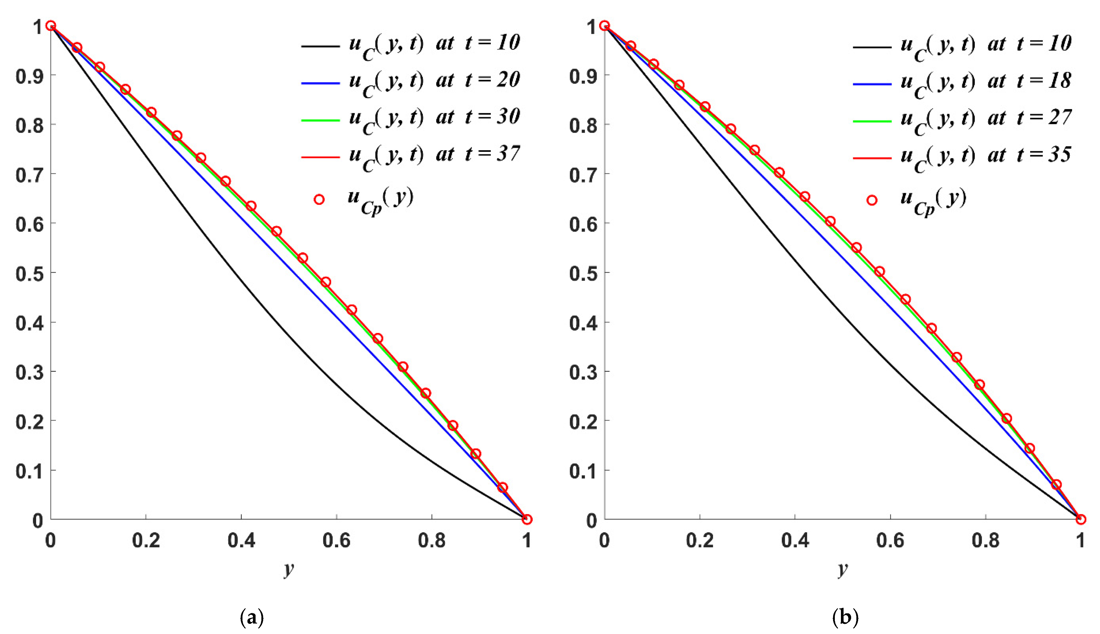
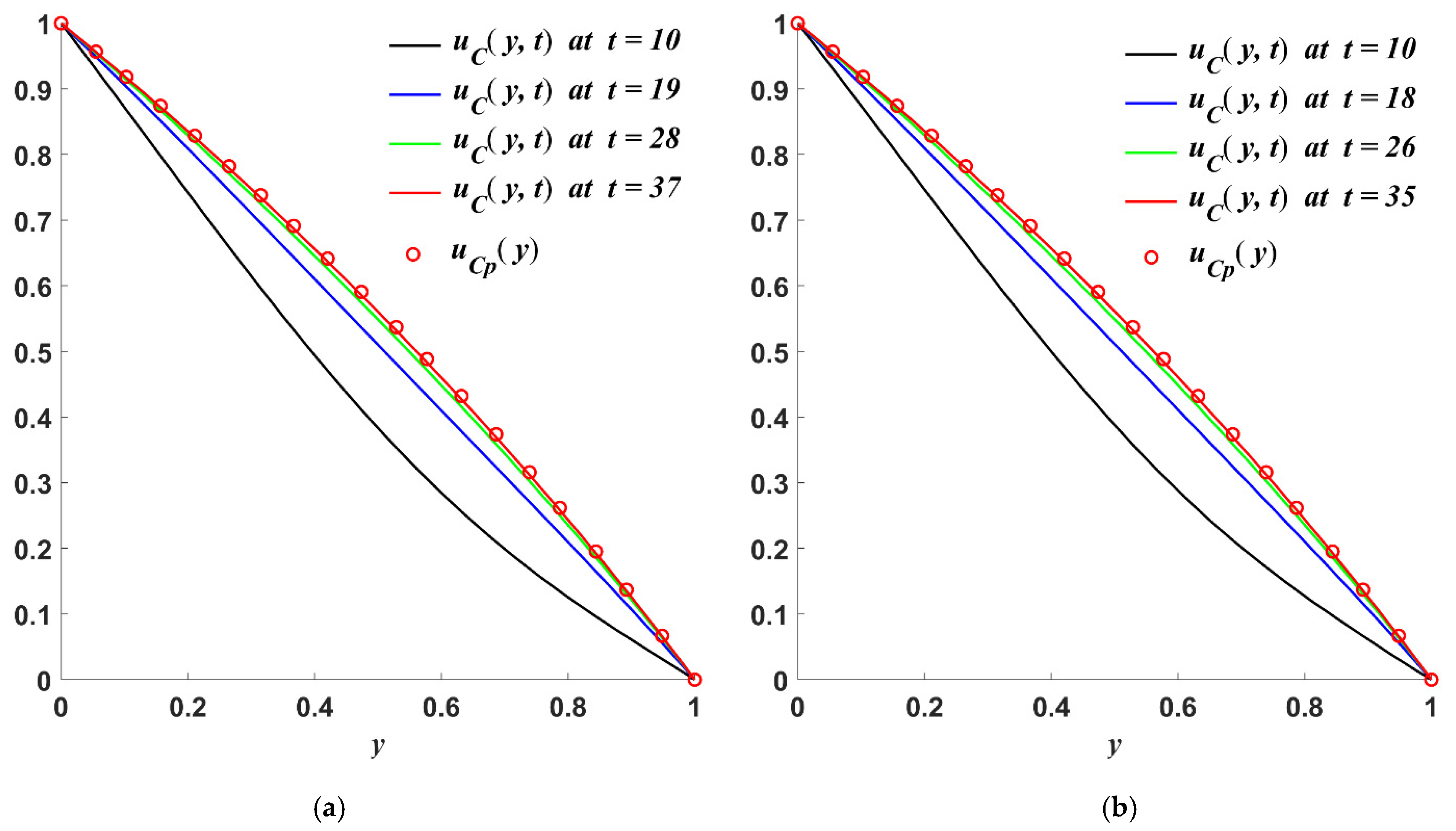
For a check of results that were here obtained, the convergence of the start-up solutions and (numerical solutions) to their steady-state components and , respectively, is proved in Figure 1, Figure 2, Figure 3 and Figure 4 for distinct values of the dimensionless pressure–viscosity coefficient and the Weissenberg number We.
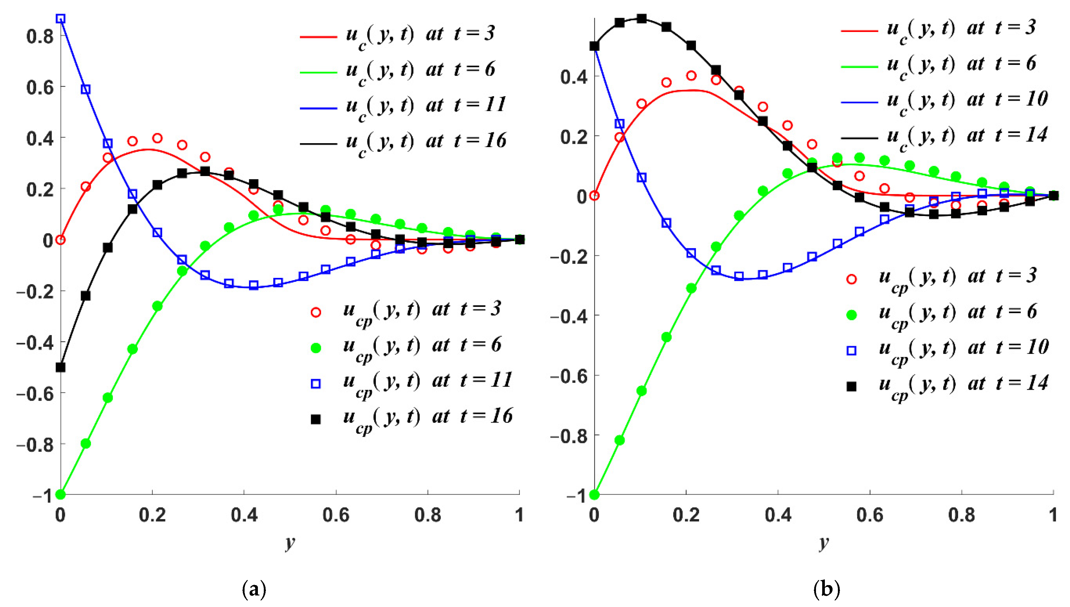
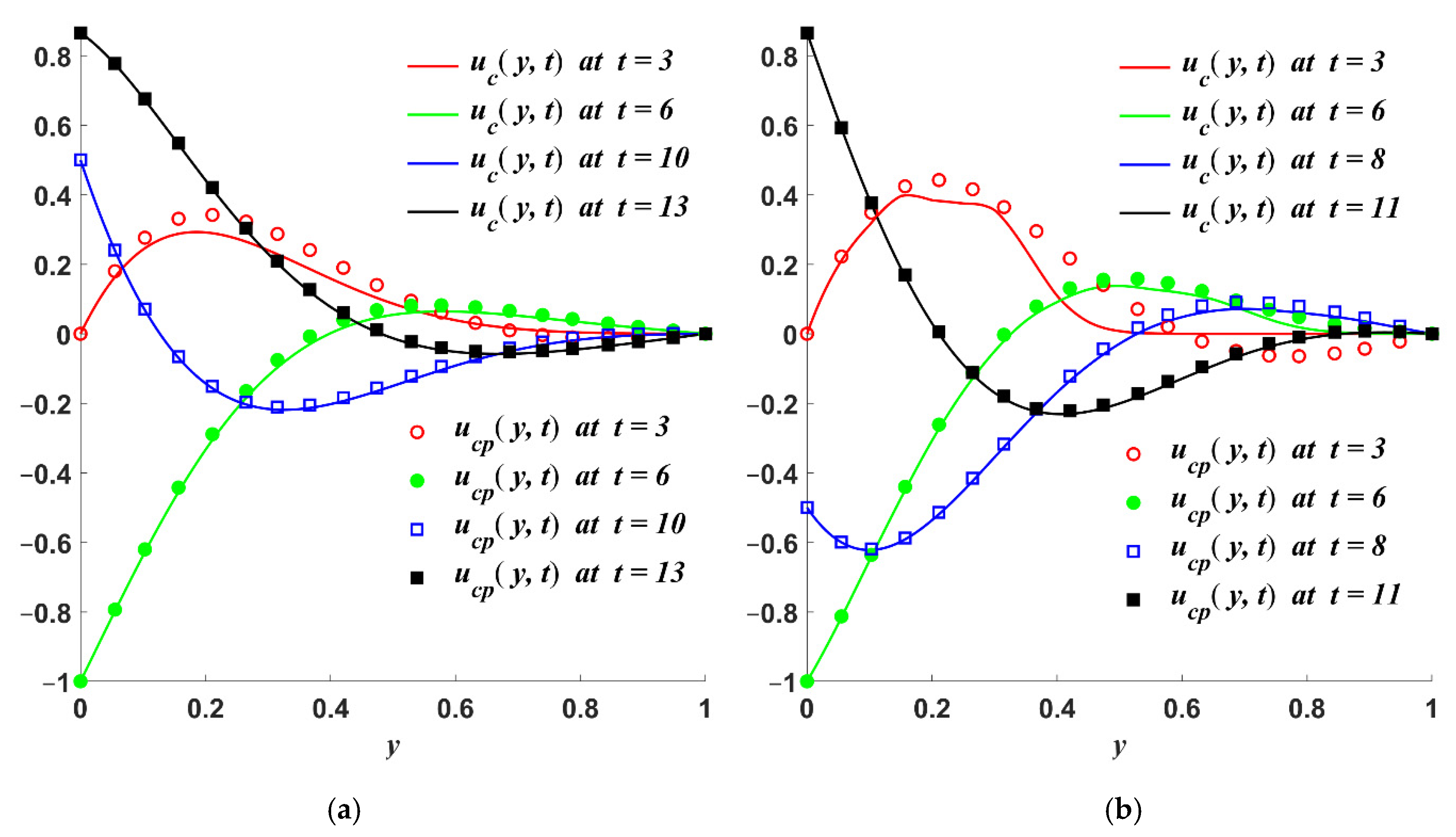
From these graphical representations, it also results that the necessary time to reach the permanent (steady) state dwindles for increasing values of or We. Consequently, the permanent state is reached later for motions of ordinary fluids, compared with fluids with pressure-dependent viscosity. It is also obtained for motions of Newtonian fluids later than UCM fluids. Figure 3 and Figure 4, as expected, reveal that the fluid velocity increases in time, and the boundary conditions are clearly satisfied.
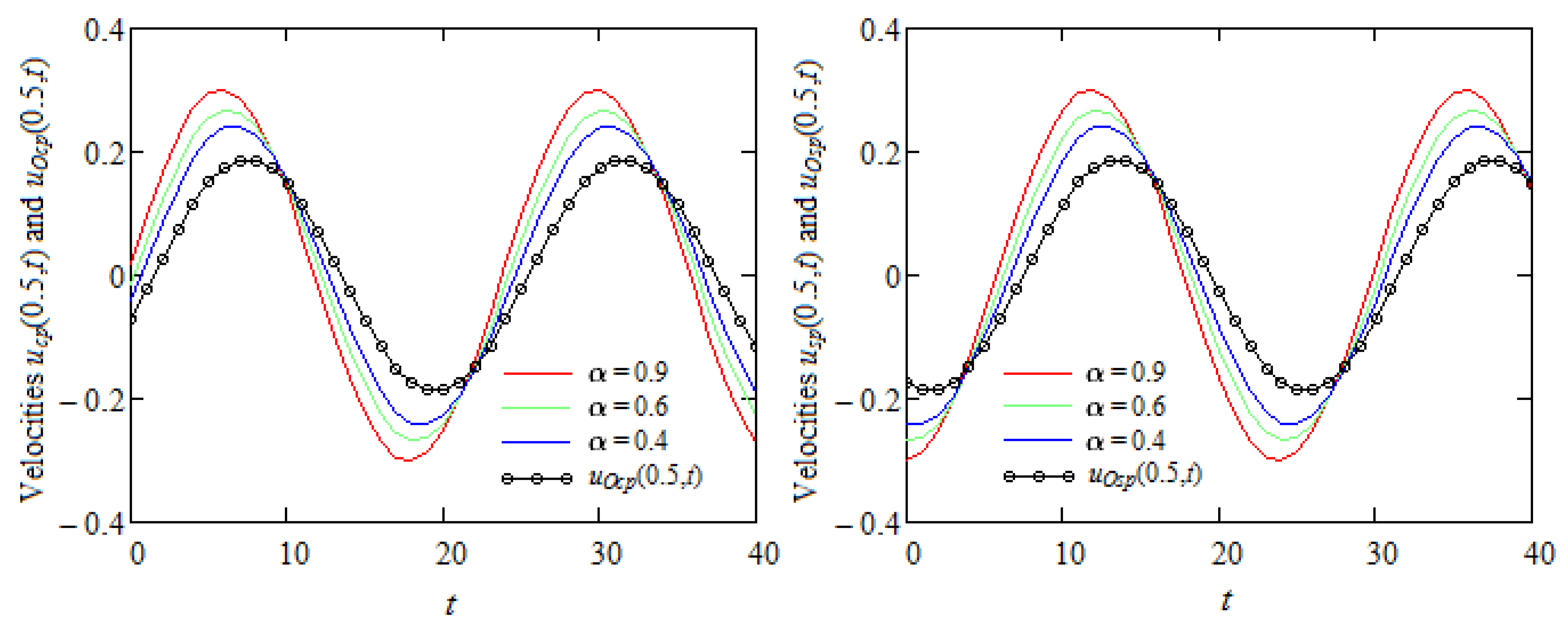
To shed light on the important characteristics regarding the fluid behavior in such motions, Figure 5, Figure 6, Figure 7, Figure 8 and Figure 9 are here prepared for and . Of particular interest for this study is the pressure–viscosity coefficient. The oscillatory specific features of the two motions and the phase difference between them are clearly underlined in Figure 5 and Figure 6. In Figure 5, the time variations in the midplane velocities are together presented at three decreasing values of , as well as .
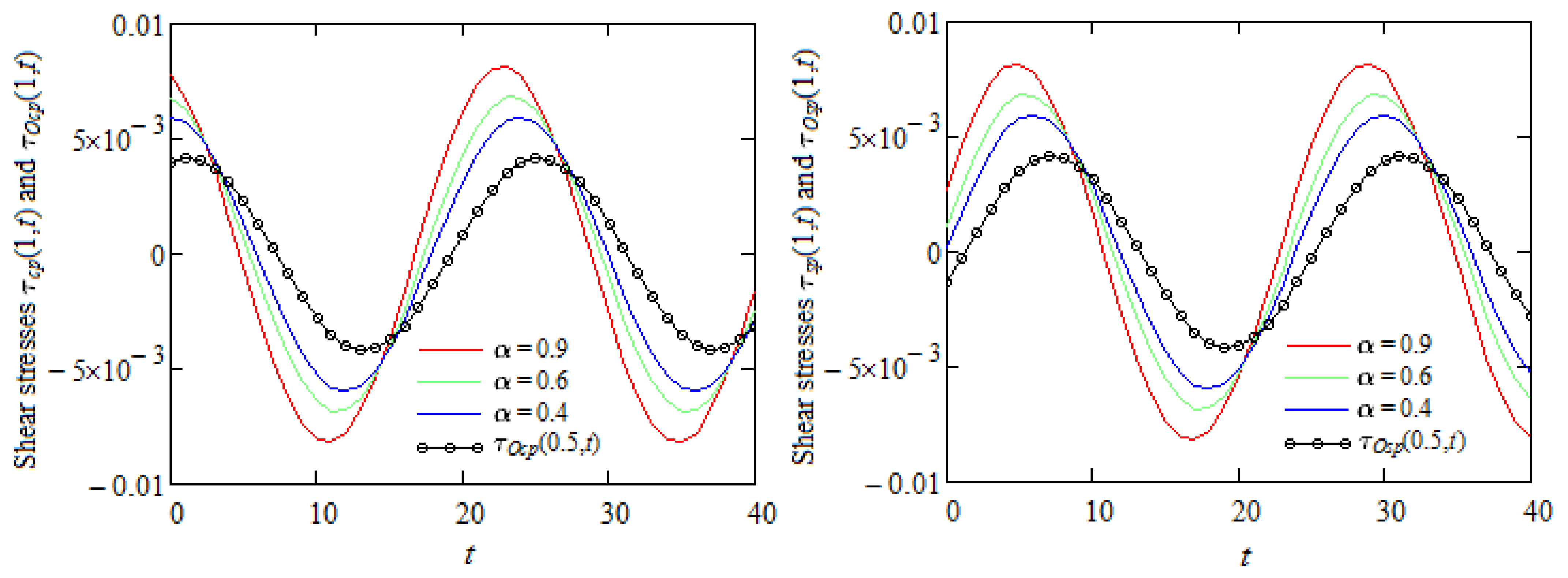
Similar graphical representations are provided in Figure 6 for the corresponding frictional forces and on the stationary wall. In all cases, as expected, the diagrams corresponding to motions of fluids with pressure-dependent viscosity tend to superpose over those of ordinary fluids. The amplitude of the oscillations corresponding to the same values of is the same for both motions. This is an increasing function with regard to the parameter . Consequently, the fluid accelerates for increasing values of and the lowest velocity corresponds to the ordinary fluids.
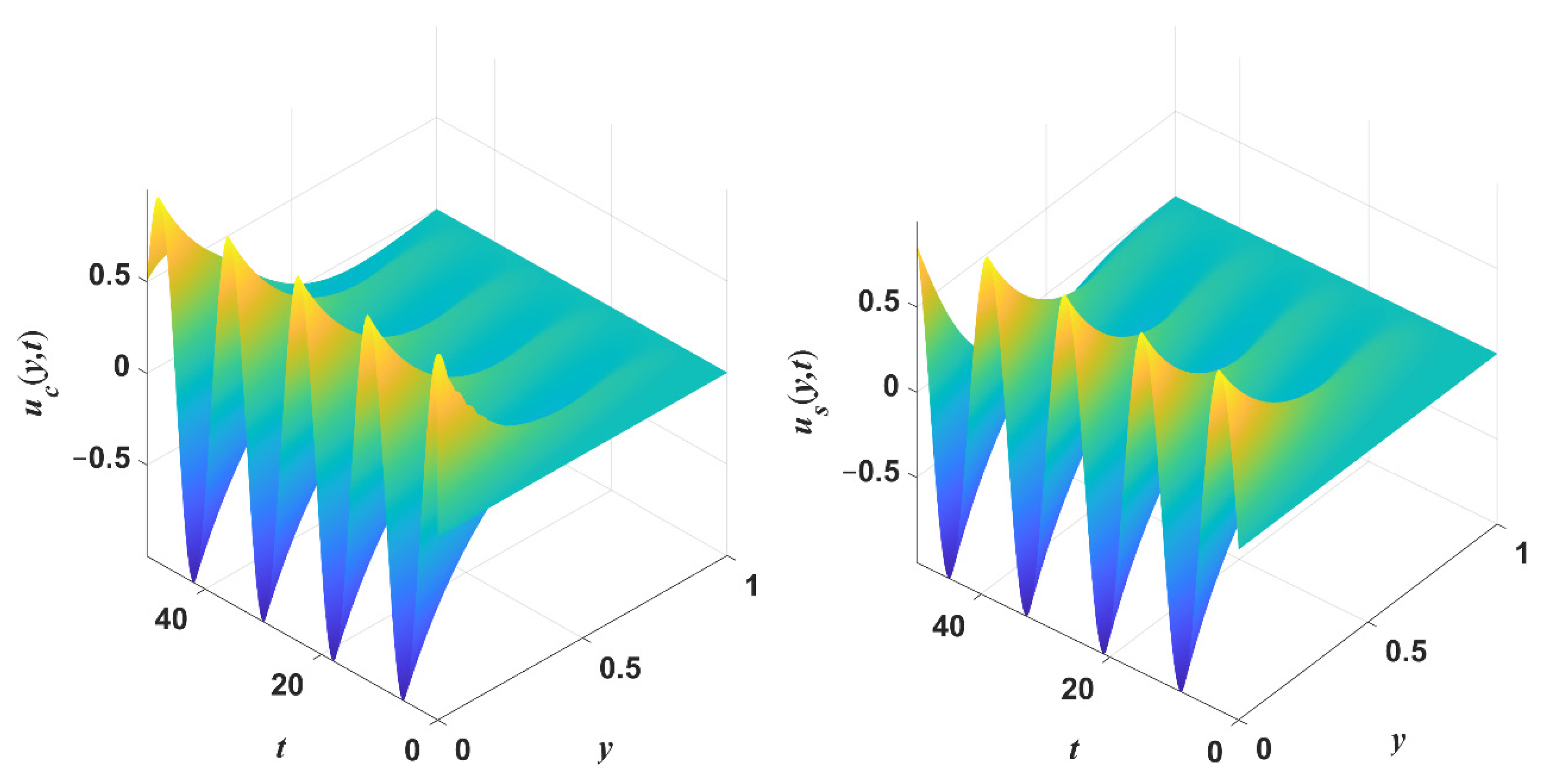
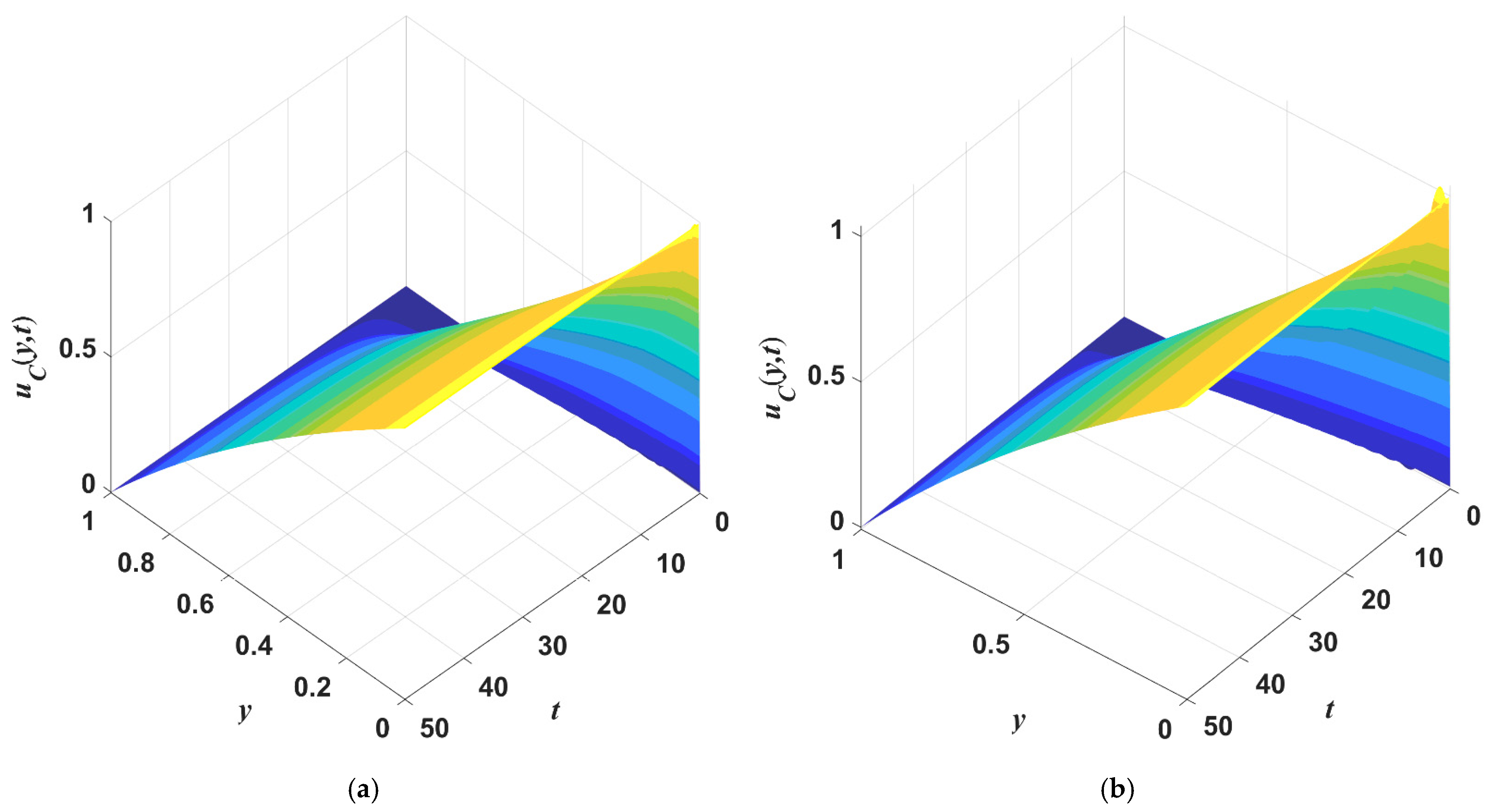
In Figure 7, for comparison, the spatial distributions of the start-up velocities and are together presented for , and . The oscillatory behavior and the phase difference between motions are easily observed, and the imposed conditions and are clearly satisfied. The spatial distribution of the velocity corresponding to the simple Couette flow is depicted in Figure 8a,b for two values of We. A careful analysis shows that is a decreasing function with regard to We. This behavior is easily explained, bearing in mind the fact that the Weissenberg number can also be interpreted as the ratio of elastic to viscous forces (see Poole [34], for instance). More specifically, if the elastic force is fixed, a reduction in We means an increase in the viscous force, which suggests a decline in the fluid velocity.
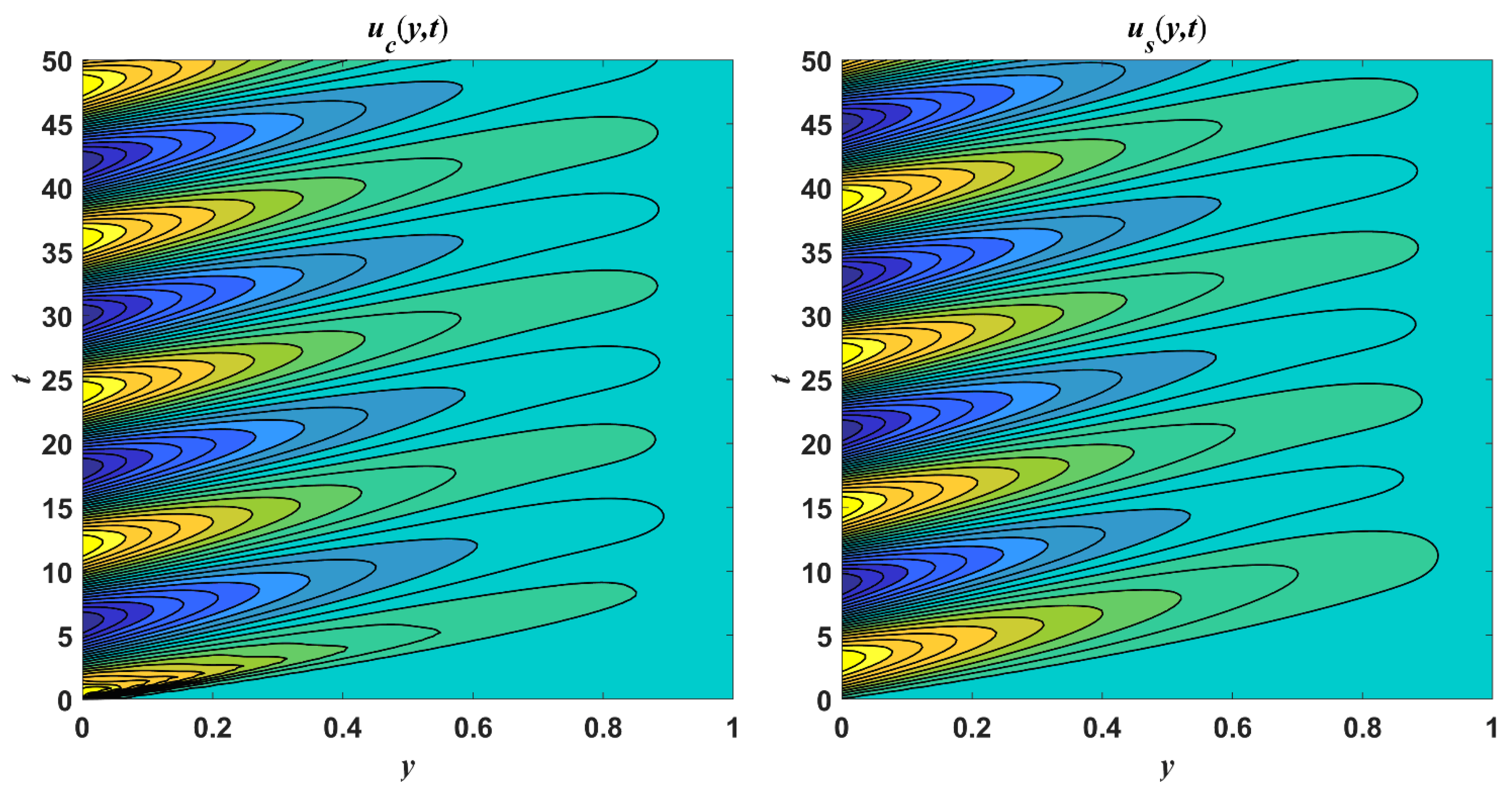
As an alternative to the first two three-dimensional graphs, the numerically computed two-dimensional contours graphs of the dimensionless start-up velocity fields and are together illustrated in Figure 9 for , and . The current graphical representations are displayed in the Parula colormap of the MATLAB software, where the maximum and minimum values of the solutions are underlined by dark yellow and dark blue colors, respectively. The alternative moving of the two separate sets of closed curves along the time t signifies the oscillatory behavior of the two solutions. The amplitude of the oscillations, as expected, diminishes for increasing values of the spatial variable y, and the notable phase difference between the two motions is due to the satisfaction of the boundary conditions.
The main outcomes that have been obtained in this work are as follows:
- –
- Closed-form expressions were established for dimensionless steady-state solutions of the modified Stokes second problem of incompressible UCM fluids with linear dependence of viscosity on the pressure;
- –
- Steady solutions for the simple Couette flow of the same fluids and steady-state solutions for the modified Stokes second problem of ordinary incompressible UCM fluids were obtained as special cases of previous results;
- –
- The dimensionless steady shear stress of the simple Couette flow of these fluids is constant on the whole flow domain, although the corresponding velocity and the normal stress are functions of the spatial variable y;
- –
- The permanent state is obtained later for motions of ordinary fluids in comparison with the fluids having pressure-dependent viscosity, as well as for incompressible Newtonian fluids, compared with incompressible UCM fluids;
- –
- Known solutions for the modified Stokes second problem of incompressible Newtonian fluids with/without pressure-dependent viscosity were immediately recovered as special cases of the present results;
- –
- The graphical representations from Figure 1, Figure 2, Figure 3 and Figure 4 and 7–9 clearly show the fluid motion is not symmetric with regard to the median plane in view of some physical reasons. However, it can become symmetric if both plates are moving in the same way. In addition, various symmetry properties are inherent at Bessel functions used in constructing solutions.
Author Contributions
Conceptualization, C.F., A.R., and D.V.; methodology, C.F., T.M.Q., and D.V.; software, T.M.Q., A.R., and D.V.; validation, C.F., T.M.Q., A.R., and D.V.; writing—review and editing, C.F. and A.R. All authors have read and agreed to the published version of the manuscript.
Funding
This research received no external funding.
Institutional Review Board Statement
Not applicable.
Informed Consent Statement
Not applicable.
Data Availability Statement
Data sharing is not applicable to this article.
Conflicts of Interest
The authors declare no conflict of interest.
Nomenclature
| Cauchy stress tensor | |
| [s] | Relaxation time |
| Extra stress tensor | |
| [Kg⋅m−1⋅s−1] | Dynamic viscosity |
| L | Velocity gradient |
| [kg⋅m−3] | Fluid density |
| I | Identity tensor |
| [m2⋅s−1] | Kinematic viscosity |
| Velocity vector | |
| [s−1] | Frequency of oscillations |
| g [ms−2] | Gravitational acceleration |
| [Kg⋅m−1⋅s−2] | Shear stress |
| [m] | Cartesian coordinates |
| [Kg⋅m−1⋅s−2] | Normal stress |
| [m⋅s−1] | Fluid velocity |
Appendix A
References
- Stokes, G.G. On the theories of the internal friction of fluids in motion, and of the equilibrium and motion of elastic solids. Trans. Camb. Philos. Soc. 1845, 8, 287–319. [Google Scholar]
- Barus, C. Note on the dependence of viscosity on pressure and temperature. Proc. Am. Acad. Arts. Sci. 1891, 27, 13–18. [Google Scholar] [CrossRef]
- Barus, C. Isothermals, isopiestics and isometrics relative to viscosity. Am. J. Sci. 1893, 45, 87–96. [Google Scholar]
- Bridgman, P.W. Viscosities to 30,000 kg/cm2. Proc. Am. Acad. Arts. Sci. 1949, 77, 117–128. [Google Scholar]
- Griest, E.M.; Webb, W.; Schiessler, R.W. Effect of pressure on viscosity of higher hydrocarbons and their mixture. J. Chem. Phys. 1958, 29, 711–720. [Google Scholar] [CrossRef]
- Bair, S.; Jarzynski, J.; Winer, W.O. The temperature, pressure and time dependence of lubricant viscosity. Tribol. Int. 2001, 34, 461–468. [Google Scholar] [CrossRef]
- Bair, S.; Kottke, P. Pressure-viscosity relationship for elastohydro-dynamics. Tribol. Trans. 2003, 46, 289–295. [Google Scholar] [CrossRef]
- Prusa, V.; Srinivasan, S.; Rajagopal, K.R. Role of pressure dependent viscosity in measurements with falling cylinder viscometer. Int. J. Non Linear Mech. 2012, 47, 743–750. [Google Scholar] [CrossRef]
- Denn, M.M. Polymer Melt Processing: Foundations in Fluid Mechanics and Heat Transfer Polymer Melt Processing; Cambridge University Press: Cambridge, UK, 2008. [Google Scholar]
- Renardy, M. Parallel shear flows of fluids with a pressure-dependent viscosity. J. Nonnewton. Fluid Mech. 2003, 114, 229–236. [Google Scholar] [CrossRef]
- Rajagopal, K.R.; Saccomandi, G.; Vergori, L. Flow of fluids with pressure and shear-dependent viscosity down an inclined plane. J. Fluid Mech. 2012, 706, 173–189. [Google Scholar] [CrossRef] [Green Version]
- Le Roux, C. Flow of fluids with pressure dependent viscosities in an orthogonal rheometer subject to slip boundary conditions. Meccanica 2009, 44, 71–83. [Google Scholar] [CrossRef]
- Martinez-Boza, F.J.; Martin-Alfonso, M.J.; Callegos, C.; Fernandez, M. High-pressure behavior of intermediate fuel oils. Energy Fuels 2011, 25, 5138–5144. [Google Scholar] [CrossRef]
- Dealy, J.M.; Wang, J. Melt Rheology and Its Applications in the Plastics Industry, 2nd ed.; Springer: Dordrecht, The Netherlands, 2013. [Google Scholar]
- Dowson, D.; Higginson, G.R. Elastohydrodynamic Lubrication: The Fundamentals of Roller and Gear Lubrication; Pergamon Press: Oxford, UK, 1966. [Google Scholar]
- Housiadas, K.D. An exact analytical solution for fluids with pressure-dependent viscosity. J. Nonnewton. Fluid Mech. 2015, 223, 147–156. [Google Scholar] [CrossRef]
- Hron, J.; Malek, J.; Rajagopal, K.R. Simple flows of fluids with pressure-dependence viscosities. Proc. Math. Phys. Eng. Sci. 2001, 457, 1603–1622. [Google Scholar] [CrossRef]
- Fusi, L. Unidirectional flows of a Herschel-Bulkley fluid with pressure-dependent rheological moduli. Eur. Phys. J. Plus 2020, 135, 544. [Google Scholar] [CrossRef]
- Rajagopal, K.R. Couette flow of fluids with pressure dependent viscosity. Int. J. Appl. Mech. Eng. 2004, 9, 573–585. [Google Scholar]
- Rajagopal, K.R. A semi-inverse problem of flows of fluids with pressure-dependent viscosities. Inverse Probl. Sci. Eng. 2008, 16, 269–280. [Google Scholar] [CrossRef]
- Prusa, V. Revisiting Stokes first and second problems for fluids with pressure-dependent viscosities. Int. J. Eng. Sci. 2010, 48, 2054–2065. [Google Scholar] [CrossRef]
- Rajagopal, K.R.; Saccomandi, G.; Vergori, L. Unsteady flows of fluids with pressure dependent viscosity. J. Math. Anal. Appl. 2013, 404, 362–372. [Google Scholar] [CrossRef]
- Kalagirou, A.; Poyiadji, S.; Georgiou, G.C. Incompressible Poiseuille flows of Newtonian liquids with a pressure-dependent viscosity. J. Nonnewton. Fluid Mech. 2011, 166, 413–419. [Google Scholar] [CrossRef]
- Akyildiz, F.T.; Siginer, D. A note on the steady flow of Newtonian fluids with pressure dependent viscosity in rectangular duct. Int. J. Eng. Sci. 2016, 104, 1–4. [Google Scholar] [CrossRef]
- Housiadas, K.D.; Georgiou, G.C. Analytical solution of the flow of a Newtonian fluid with pressure-dependent viscosity in a rectangular duct. Appl. Math. Comput. 2018, 322, 123–128. [Google Scholar] [CrossRef]
- Fetecau, C.; Bridges, C. Analytical solutions of some unsteady flows of fluids with linear dependence of viscosity on the pressure. Inverse Probl. Sci. Eng. 2021, 29, 378–395. [Google Scholar] [CrossRef]
- Vieru, D.; Fetecau, C.; Bridges, C. Analytical solutions for a general mixed boundary value problem associated to motions of fluids with linear dependence of viscosity on the pressure. Int. J. Appl. Mech. Eng. 2020, 25, 181–197. [Google Scholar] [CrossRef]
- Karra, S.; Prusa, V.; Rajagopal, K.R. On Maxwell fluid with relaxation time and viscosity depending on the pressure. Int. J. Non Linear Mech. 2011, 46, 819–827. [Google Scholar] [CrossRef] [Green Version]
- Fetecau, C.; Rauf, A.; Qureshi, T.M.; Mehmood, O.U. Analytical solutions of upper-convected Maxwell fluid flow with exponential dependence of viscosity on the pressure. Eur. J. Mech. B Fluids 2021, 88, 148–159. [Google Scholar] [CrossRef]
- Evans, J.D. High Weissenberg number boundary layer structures for UCM fluids. Appl. Math. Comput. 2020, 387, 124952. [Google Scholar] [CrossRef]
- Menon, E.S. Fluid flow in pipes. In Transmission Pipeline Calculations and Simulations Manual; Elsevier: Amsterdam, The Netherlands, 2015; pp. 149–234. [Google Scholar]
- Erdogan, M.E. On the unsteady unidirectional flows generated by impulsive motion of a boundary or sudden application of a pressure gradient. Int. J. Non Linear Mech. 2002, 37, 1091–1106. [Google Scholar] [CrossRef]
- Fetecau, C.; Ellahi, R.; Sait, S.M. Mathematical analysis of Maxwell fluid flow through a porous plate channel induced by a constantly accelerating or oscillating wall. Mathematics 2021, 9, 90. [Google Scholar] [CrossRef]
- Poole, R.J. The Deborah and Weissenberg numbers. Rheol. Bull. 2012, 53, 32–39. [Google Scholar]
Figure 1.
Graphical representations of and (numerical solutions) for , increasing values of the time t and two values of . (a) . (b) .
Figure 1.
Graphical representations of and (numerical solutions) for , increasing values of the time t and two values of . (a) . (b) .

Figure 2.
Graphical representations of and (numerical solutions) for , increasing values of the time t and two values of We. (a) . (b) .
Figure 2.
Graphical representations of and (numerical solutions) for , increasing values of the time t and two values of We. (a) . (b) .

Figure 3.
Graphical representations of and (numerical solutions) for , increasing values of the time t and two values of . (a) . (b) .
Figure 3.
Graphical representations of and (numerical solutions) for , increasing values of the time t and two values of . (a) . (b) .

Figure 4.
Graphical representations of and (numerical solutions) for , increasing values of the time t and two values of We. (a) . (b) .
Figure 4.
Graphical representations of and (numerical solutions) for , increasing values of the time t and two values of We. (a) . (b) .

Figure 5.
Time evolution of the velocities , (for three decreasing values of ) and , , for .

Figure 6.
Time evolution of the shear stresses , (for three decreasing values of ) and , , for .

Figure 7.
Spatial distribution of the dimensionless start-up velocities and (numerical solutions) for and .
Figure 7.
Spatial distribution of the dimensionless start-up velocities and (numerical solutions) for and .

Figure 8.
Spatial distribution of the dimensionless start-up velocity (numerical solution) for , and two values of We. (a) . (b) .
Figure 8.
Spatial distribution of the dimensionless start-up velocity (numerical solution) for , and two values of We. (a) . (b) .

Figure 9.
Contours diagrams of the dimensionless start-up velocities and (numerical solutions) for and .
Figure 9.
Contours diagrams of the dimensionless start-up velocities and (numerical solutions) for and .

Publisher’s Note: MDPI stays neutral with regard to jurisdictional claims in published maps and institutional affiliations. |
© 2022 by the authors. Licensee MDPI, Basel, Switzerland. This article is an open access article distributed under the terms and conditions of the Creative Commons Attribution (CC BY) license (https://creativecommons.org/licenses/by/4.0/).
Share and Cite
MDPI and ACS Style
Fetecau, C.; Qureshi, T.M.; Rauf, A.; Vieru, D. On the Modified Stokes Second Problem for Maxwell Fluids with Linear Dependence of Viscosity on the Pressure. Symmetry 2022, 14, 219. https://doi.org/10.3390/sym14020219
AMA Style
Fetecau C, Qureshi TM, Rauf A, Vieru D. On the Modified Stokes Second Problem for Maxwell Fluids with Linear Dependence of Viscosity on the Pressure. Symmetry. 2022; 14(2):219. https://doi.org/10.3390/sym14020219
Chicago/Turabian StyleFetecau, Constantin, Tahir Mushtaq Qureshi, Abdul Rauf, and Dumitru Vieru. 2022. "On the Modified Stokes Second Problem for Maxwell Fluids with Linear Dependence of Viscosity on the Pressure" Symmetry 14, no. 2: 219. https://doi.org/10.3390/sym14020219
Note that from the first issue of 2016, this journal uses article numbers instead of page numbers. See further details here.