
Partial Asymmetry Measures for Square Contingency Tables

1
Innovative and Clinical Research Promotion Center, Gifu University Hospital, Gifu City 501-1194, Gifu, Japan
2
Department of Biostatistics, Yokohama City University School of Medicine, Yokohama City 236-0004, Kanagawa, Japan
3
Department of Information Sciences, Faculty of Science and Technology, Tokyo University of Science, Noda City 278-8510, Chiba, Japan
4
Department of Information Sciences, Faculty of Information Sciences, Meisei University, Hino City 191-0042, Tokyo, Japan
*
Author to whom correspondence should be addressed.
Symmetry 2022, 14(9), 1936; https://doi.org/10.3390/sym14091936
Submission received: 19 August 2022
/
Revised: 13 September 2022
/
Accepted: 14 September 2022
/
Published: 17 September 2022
(This article belongs to the Section Mathematics)
Abstract
:In square contingency table analysis, we consider a partial measure that represents the degree of departure from symmetry for each of several pairs. It may be useful to pool the values of the measure into a single summary measure of partial asymmetry. We show that the estimator of partial measures is asymptotically mutually independent for a large sample size. The present paper proposes a symmetry measure in the class of weighted averages that is different from previous studies. The proposed measure is an approximation of the measure in the class of weighted averages that has the smallest variance.
1. Introduction
In categorical data analysis, contingency tables are a basic tool used to examine the relationship between row and column categories. For example, the Pearson statistic is commonly used to test the null hypothesis of statistical independence (Agresti [1] [p. 75]). When statistical independence is rejected, we are interested in describing the association between the row and column categories. Summary measures of association have been proposed, such as the Cramér V, gamma, and uncertainty coefficient. For details, see for instance Agresti [1] [Sec. 2.4] and Bishop et al. [2] [Sec. 11.3]. Additionally, the recent development of association measures is described, for example, in Beh et al. [3], Lombardo [4], Wei and Kim [5], Wei and Kim [6], Zhang et al. [7], and Wei et al. [8].
Contingency tables with the same row and column classifications are called square contingency tables. These tables are used for unaided distance vision data, social mobility data, and longitudinal data in biomedical research. The analysis of square contingency tables considers the issue of symmetry rather than independence because it is not sensible to treat these data as independent.
Bowker [9] introduced the simple symmetry model and proposed a test for the hypothesis of symmetry. When the symmetry model fits the given data poorly, we are interested in measuring the degree of departure from symmetry. Tomizawa [10] proposed a measure that represents the degree of departure from symmetry expressed using the Shannon entropy or Kullback–Leibler information. In the real world, the Shannon entropy is widely applied as a measure of complexity, for example in Fernandes and Araújo [11]. The measure lies between 0 and 1, and its value equals 0 if and only if the symmetry model holds. Additionally, the degree of departure from symmetry increases as the value of the measure increases.
In the present paper, we propose a measure that represents the degree of departure from symmetry using a different approach. We also consider a partial measure that represents the degree of departure from symmetry for each of several pairs. If the asymmetry appears to be similar in the various pairs, it may be useful to pool the values of the measure into a single summary measure of partial asymmetry. In an analogous manner to Agresti [12] [p. 170], we consider taking a weighted average of the sample values as a summary measure. The properties of the proposed measure are given, and it has a characteristic that is different from that of Tomizawa’s measure.
The rest of this paper is organized as follows. Section 2 describes the background of this study by reviewing previous research. Section 3 proposes the new measure that represents the degree of departure from symmetry. Section 4 shows some numerical examples and discusses the difference between the estimate of and the estimate of the proposed measure. Section 5 gives an example involving the cross-classification of mothers’ and fathers’ birth orders. Section 6 contains concluding remarks.
2. Review of Previous Research
Consider an square contingency table having the same row and column classifications. Let denote the probability that an observation will fall in the th cell of the table . The simple symmetry model introduced by Bowker [9] is defined by
This model indicates the symmetry structure with respect to the cell probabilities. Bowker [9] proposed a test for the hypothesis of symmetry.
When the symmetry model does not hold for a given dataset, we are interested in evaluating the degree of departure from symmetry. Assuming is not equal to zero for , the measure is defined as
where . The measure has three properties: (i) ; (ii) the table has a symmetrical structure if and only if ; (iii) there is a structure for which either or for if and only if .
Let for . The conditional probability that an observation falls in cell or in the table is . It should be noted that the symmetry model can be expressed as
The measure can be expressed as
where
It should be noted that is the normalized Kullback–Leibler information between and . That is, the measure is the weighted average of .
We review in . The partial measure represents the degree of departure from symmetry for a pair of symmetric cells because: (i) ; (ii) there is a symmetrical structure for the pair of and cells if and only if ; (iii) there is a structure for which either or for the pair of and cells if and only if . That is, the measure expresses partial asymmetry.
3. The Proposed Measure
Let denote the observed frequency in the th cell of the table (; ). We assume that have a multinomial distribution:
where . Let be the vector
where
Furthermore, let us define the vector in terms of s in the same way as . Let denote the sample version of . Namely, the estimated is given as
where and . Let be the vector:
and we define the vector in terms of s in a similar manner to . From Appendix A, is asymptotically distributed as normal with mean and covariance matrix
where
It should be noted that the set is asymptotically mutually independent for large n.
We consider the weighted average of , that is
where the weights satisfy all and . We see from Appendix A that is asymptotically distributed normal as independently. Thus, the measure has an asymptotically normal distribution with mean
and variance
In an analogous manner to Agresti [12] [p. 170], we derive the weights so as to minimize the variance of with the constraint that all and . From Appendix B, we obtain
Then, we consider the following measure, which represents the degree of departure from symmetry:
The measure (17) has the smallest variance among measures in the class of weighted averages given in Equation (13). It should be noted that we should estimate the variances because these are unknown.
We propose the estimated measure as follows:
where is given by with replaced by . The proposed measure approximates the measure in the class of weighted averages that has the smallest variance. The estimated measure is the weighted average of using the weights , where . On the other hand, the proposed measure is the weighted average of using the weights . It should be noted that (i) indicates the estimated conditional probability that the observation falls in or cells on the condition that the observation falls in off-diagonal cells and (ii) the weight becomes larger as the variance of partial measure decreases.
4. Numerical Examples
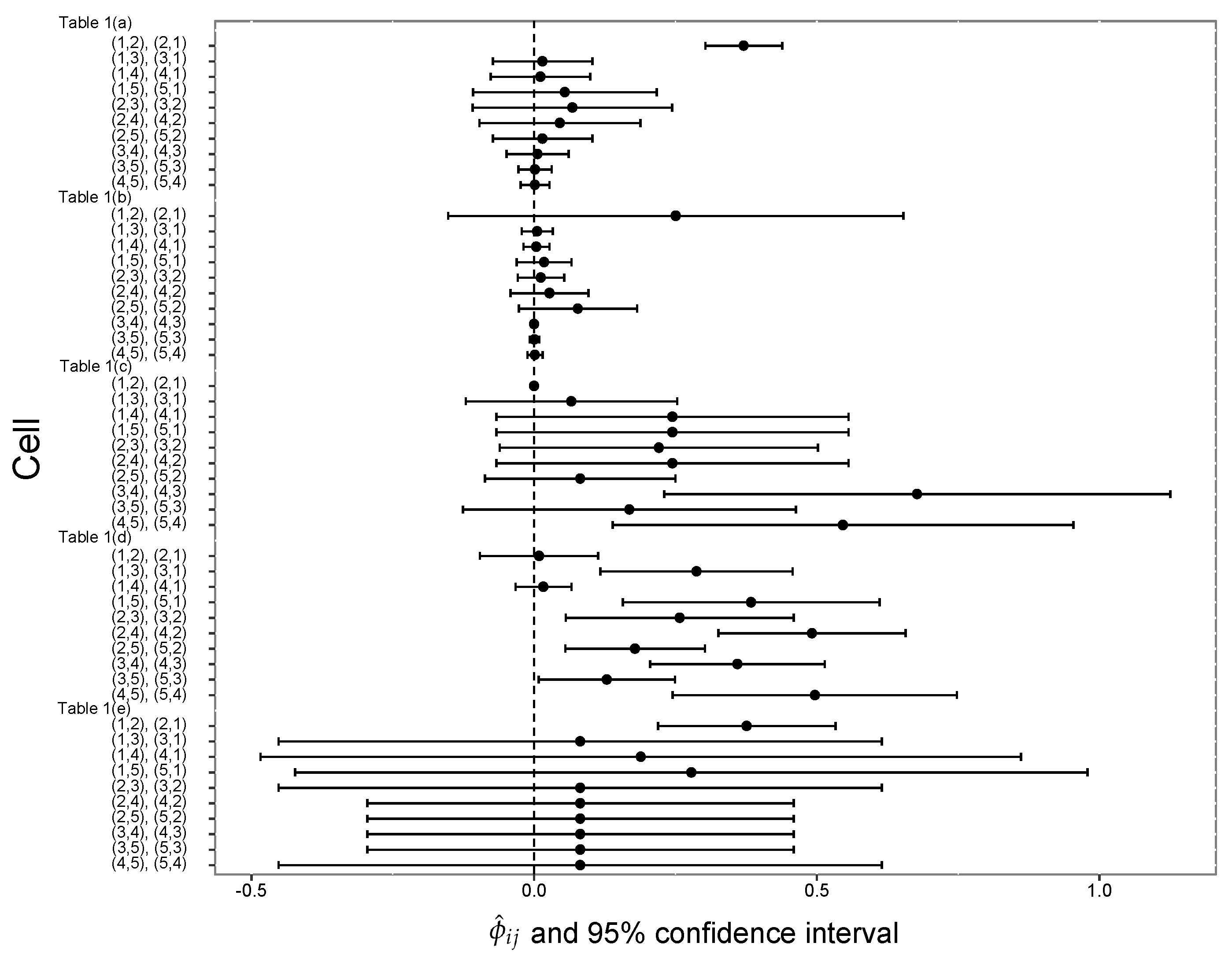
The objective is to confirm the difference in the single summary measure for symmetry by comparing the weights and . Consider the artificial data in Table 1(a)–(d) with and Table 1(e) with . Table 1(a)–(d) are generated from the random numbers of the multinomial distribution based on the cell probability tables (a), (b), (c), and (d) in Table 2, respectively. Table 1(e) is generated from the random numbers of the multinomial distribution based on the cell probability table in Table 2(a). The artificial cell probability tables of Table 2 focus in particular on the probabilities of cells and , and the four patterns (a), (b), (c), and (d) are set according to the combination of partial symmetry/asymmetry. We shall apply the partial measure . Table 3 shows the estimated partial measure , estimated variance , confidence interval for , estimated weights for , and estimated weights for . Figure 1 visualizes the estimated partial measure and confidence interval for . The confidence interval for applied to the data in Table 1(a) does not contain zero, indicating that there is a partially asymmetric structure in cells and . Furthermore, the confidence interval for does not overlap with the confidence intervals for for any other pair of cells, indicating that cells and are partially asymmetric compared to every other pair of cells. The of is remarkably smaller than the of , and the value of is smaller than that of . The value of applied to the data in Table 1(b) is as large as the value of applied to the data in Table 1(a). However, it cannot be shown that there is a partially asymmetric structure in cells and in Table 1(b) because the confidence interval for is wide and contains zero. Both and in Table 1(b) have small values of and , and in particular, the for is remarkably small.
On the other hand, the value of applied to the data in Table 1(c) indicates that there is a partially symmetric structure in cells and because the value of is small and the confidence interval for the contains zero. In addition, the in Table 1(c) is large, indicating that the weight of is larger when the pair of cells is more frequent than others and has a partially symmetric structure. Both and applied to the data in Table 1(c) are close to zero because of the greater weight of the pair of cells and that show partial symmetry compared to the pairs of cells and and and that show partial asymmetry. The values of applied to the data in Table 1(d) indicate that the pair of cells and and the pair of cells and both have a partially symmetric structure because the confidence intervals of and include zero. It can be seen that the values of and for are similar, while the value of for is large compared to .
The value of applied to the data in Table 1(e) is about the same as the value applied to the data in Table 1(a), but the confidence interval is wider due to the smaller sample size, making it relatively difficult to conclude partial asymmetry for the pair of cells and . The magnitude of applied to Table 1(e) does not differ much from the results applied to Table 1(a). However, the values of and are greater when applied to Table 1(e) than Table 1(a). It should be noted that the weight becomes larger as the variance of the partial measure decreases, and the weight becomes larger as the proportion increases.
5. Example
Consider the data in Table 4, derived from the national survey on educational attitudes of high school students and their mothers in Japan in 2012. To clarify the structure of educational inequalities in contemporary Japanese society and the actual educational awareness of parents and children, a postal survey was conducted among second-year high school students and their mothers throughout Japan, using the same framework as the national survey on the educational awareness of high school students and their mothers conducted in November 2002. The data describe the cross-classification of mothers’ and fathers’ birth orders. For example, for the 179 high school students whose mothers’ birth order is “First” and whose fathers’ birth order is “Second”, the mother is the eldest daughter and the father is the second son. The partial symmetry of cells and means that the probability of high school students whose mother is the eldest daughter and whose father is the second son is equal to that of high school students whose mother is the second daughter and whose father is the eldest son.
Let and denote the likelihood ratio and Pearson’s chi-squared statistics for testing the goodness of fit of the symmetry model, i.e., and . For large samples, and have a chi-squared null distribution with degrees of freedom. From and with six degrees of freedom for the data in Table 4, these values indicate the lack of a symmetrical structure. Note that the exact test introduced by West [13] is well known as a test for the contingency table including structural zeros. As the proposed measure does not require the frequency of the diagonal components, West’s test was also conducted assuming that the diagonal components are structural zeros. The simulated p-value from West’s test is 0.085, which indicates that the rows and columns are independent. The value of is 0.0184, and the 95% confidence interval is (0.000003, 0.036719), which does not include zero.
Next, we measured the degree of departure from partial symmetry for each pair of cells. We shall apply the partial measure for the data in Table 4. Table 5 shows the estimated values for and , confidence intervals for , estimated weights and , and estimated measures and . According to the magnitudes of the estimates, can explain the partial symmetry for each pair of cells in Table 4. The 95% confidence interval for the for all pairs of cells contains zero, which indicates that there is a partially symmetrical structure in each birth order category in the mother–father pairs.
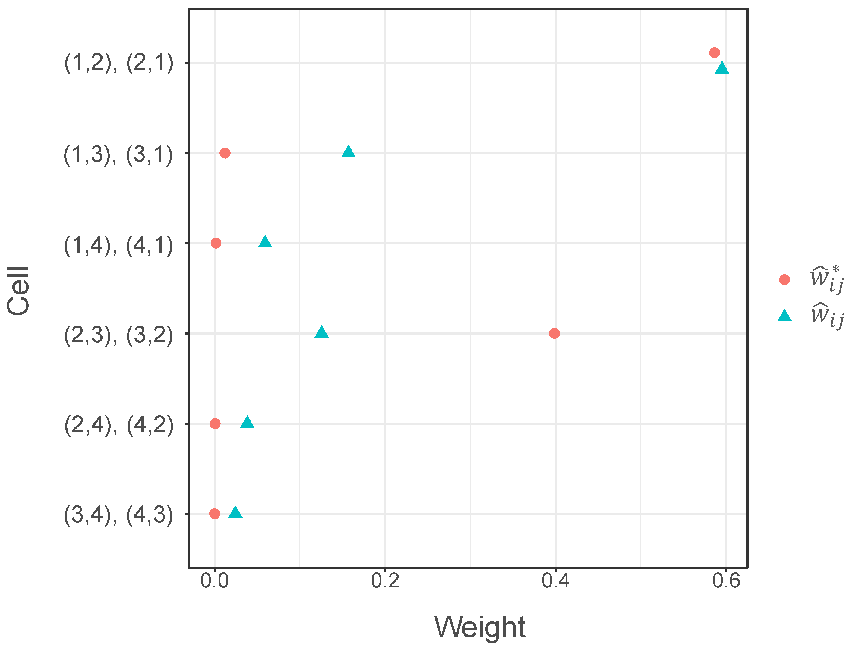
Furthermore, the estimated departure from symmetry is smaller with , which uses different weights than . Figure 2 plots estimated weights and . Cells and have similar frequencies and are more frequent than the other cells. Then, weights and are similar and large. On the other hand, the pair of cells and have similar frequencies, but are less frequent than the pair of cells and . In such cases, is larger than . Therefore, has a higher weight than when the pair of cells has a lower frequency than another pair of cells and when the cells have similar frequencies. Conversely, is smaller than when the frequencies are different, as in the pair of cells and . Since the weights and take different values, the single summary measures and also take different values. As mentioned above, there is a partially symmetrical structure in each birth order category in the mother–father pairs. Then, the proposed measure may be reasonable to express the degree of departure from symmetry.
6. Concluding Remarks
We proposed a partial measure to express the degree of departure from partial symmetry. The measure was constructed as the weighted average of partial measures expressed using the Shannon entropy or Kullback–Leibler information. The composition of the proposed measure is similar to that of the measure proposed by Tomizawa [10] in the sense that they are classes of weighted averages. However, they differ in that the weights multiplied by the partial measure are constructed so as to minimize the measure’s variance. This measure increase with the degree of departure from symmetry, allowing us to see how far away the probability structure of the contingency table is from complete asymmetry.
The measures and are invariant under the arbitrary simultaneous permutations of row and column categories, and therefore, it is possible to apply these measures to analyze the data on a nominal scale, as well as on an ordinal scale if one cannot use the information about the order in which the categories are listed.
We compared the weights used to construct the measures and . Those used to construct are large when the frequency of the pair of cells is high compared to others. On the other hand, the weight of is higher when the frequency of the pair of cells is higher than others and when the structure is partially symmetric. Conversely, when the frequency of the pair of cells is lower than others and the structure is partially asymmetric, the weights of are smaller than those of .
In the present study, confidence intervals for partial measures were used to interpret the partially asymmetric structure of the data. Alternatively, global tests for the null hypothesis that all are equally zero, and multiplicity correction for paired comparisons also need to be considered and are left as future works.
We should note, however, that cannot be calculated if any of the off-diagonal cells are zero. As such, the proposed measure should be used for contingency tables with large sample sizes.
Author Contributions
Conceptualization, T.I., K.T. and K.Y.; methodology, T.I., K.T. and K.Y.; software, T.I.; validation, K.T.; formal analysis, T.I.; investigation, T.I.; writing—original draft preparation, T.I., K.T. and K.Y.; writing—review and editing, T.I., K.T., K.Y. and S.T.; visualization, T.I.; supervision, S.T.; project administration, K.T.; All authors have read and agreed to the published version of the manuscript.
Funding
This research received no external funding.
Data Availability Statement
Not applicable.
Acknowledgments
The data, for example, in Section 5, the national survey on educational attitudes of high school students and their mothers in Japan in 2012, were provided by the Social Science Japan Data Archive, Center for Social Research and Data Archives, Institute of Social Science, The University of Tokyo. Furthermore, the authors are grateful to an Associate Editor and three Referees for their constructive comments and useful suggestions.
Conflicts of Interest
The authors declare no conflict of interest.
Appendix A
From the central limit theorem, is asymptotically distributed as normal , where is the matrix
where denotes a diagonal matrix with the ith element of as the ith diagonal element. Then, we also obtain
where is the matrix. Thus, is asymptotically distributed as normal , where
Let be the vector:
where . Noting that is a function of only , we obtain
It should be noted that is the matrix and is the matrix. By obtaining , we can see that is expressed as
where is the matrix:
where
Thus, is also expressed as follows:
where
Appendix B
Let be the vector:
Then, the measure (13) is expressed as .
Then, we can obtain the following so as to minimize with the constraint that is unity ( is the vector of 1 elements):
References
- Agresti, A. Categorical Data Analysis, 3rd ed.; Wiley: Hoboken, NJ, USA, 2013. [Google Scholar]
- Bishop, Y.M.M.; Fienberg, S.E.; Holl, P.W. Discrete Multivariate Analysis: Theory and Practice; The MIT Press: Cambridge, MA, USA, 1975. [Google Scholar]
- Beh, E.J.; Simonetti, B.; D’Ambra, L. Partitioning a non-symmetric measure of association for three-way contingency tables. J. Multivar. Anal. 2007, 98, 1391–1411. [Google Scholar] [CrossRef]
- Lombardo, R. Three-way association measure decompositions: The Delta index. J. Stat. Plan. Inference 2011, 141, 1789–1799. [Google Scholar] [CrossRef]
- Wei, Z.; Kim, D. Subcopula-based measure of asymmetric association for contingency tables. Stat. Med. 2017, 36, 3875–3894. [Google Scholar] [CrossRef] [PubMed]
- Wei, Z.; Kim, D. Measure of asymmetric association for ordinal contingency tables via the bilinear extension copula. Stat. Probab. Lett. 2021, 178, 109183. [Google Scholar] [CrossRef]
- Zhang, L.; Lu, D.; Wang, X. The essential dependence for a group of random vectors. Commun. Stat.-Theory Methods 2021, 50, 5836–5872. [Google Scholar] [CrossRef]
- Wei, Z.; Kim, D.; Conlon, E.M. A Bayesian approach to the analysis of asymmetric association for two-way contingency tables. Comput. Stat. 2022, 37, 1311–1338. [Google Scholar] [CrossRef]
- Bowker, A.H. A test for symmetry in contingency tables. J. Am. Stat. Assoc. 1948, 43, 572–574. [Google Scholar] [CrossRef] [PubMed]
- Tomizawa, S. Two kinds of measures of departure from symmetry in square contingency tables having nominal categories. Stat. Sin. 1994, 4, 325–334. [Google Scholar]
- Fernandes, L.H.S.; Araújo, F.H.A. Taxonomy of commodities assets via the complexity-entropy causality plane. Chaos Solitons Fractals 2020, 137, 109909. [Google Scholar] [CrossRef]
- Agresti, A. Analysis of Ordinal Categorical Data; Wiley: New York, NY, USA, 1984. [Google Scholar]
- West, L.J.; Hankin, R.K.S. Exact tests for two-way contingency tables with structural zeros. J. Stat. Softw. 2008, 28, 1–19. [Google Scholar] [CrossRef] [Green Version]
Figure 1.
Estimate of measure and approximate 95% confidence interval for applied to Table 1.
Figure 1.
Estimate of measure and approximate 95% confidence interval for applied to Table 1.

Figure 2.
The weight for each pair of symmetric cells obtained by applying the proposed method and Tomizawa [10] to Table 4.


Table 1.
Artificial data.
| (a) | (1) | (2) | (3) | (4) | (5) |
| (1) | 37 | 544 | 12 | 7 | 8 |
| (2) | 102 | 26 | 15 | 15 | 12 |
| (3) | 9 | 8 | 29 | 10 | 11 |
| (4) | 9 | 9 | 12 | 40 | 12 |
| (5) | 14 | 9 | 10 | 11 | 29 |
| (b) | (1) | (2) | (3) | (4) | (5) |
| (1) | 47 | 11 | 37 | 44 | 48 |
| (2) | 3 | 38 | 34 | 37 | 49 |
| (3) | 44 | 44 | 52 | 56 | 48 |
| (4) | 38 | 25 | 55 | 45 | 47 |
| (5) | 35 | 25 | 51 | 43 | 44 |
| (c) | (1) | (2) | (3) | (4) | (5) |
| (1) | 33 | 316 | 13 | 18 | 18 |
| (2) | 321 | 37 | 20 | 18 | 20 |
| (3) | 7 | 6 | 26 | 16 | 14 |
| (4) | 5 | 5 | 1 | 30 | 19 |
| (5) | 5 | 10 | 5 | 2 | 35 |
| (d) | (1) | (2) | (3) | (4) | (5) |
| (1) | 39 | 4 | 70 | 42 | 50 |
| (2) | 5 | 34 | 45 | 110 | 84 |
| (3) | 17 | 12 | 54 | 103 | 63 |
| (4) | 31 | 14 | 20 | 39 | 48 |
| (5) | 9 | 29 | 26 | 6 | 46 |
| (e) | (1) | (2) | (3) | (4) | (5) |
| (1) | 7 | 103 | 1 | 1 | 4 |
| (2) | 19 | 10 | 2 | 2 | 4 |
| (3) | 2 | 1 | 6 | 2 | 2 |
| (4) | 3 | 4 | 4 | 5 | 2 |
| (5) | 1 | 2 | 4 | 1 | 8 |
Table 2.
Artificial cell probability tables.
| (a) | (1) | (2) | (3) | (4) | (5) |
| (1) | 0.030 | 0.570 | 0.010 | 0.010 | 0.010 |
| (2) | 0.010 | 0.030 | 0.010 | 0.010 | 0.010 |
| (3) | 0.010 | 0.010 | 0.030 | 0.010 | 0.010 |
| (4) | 0.010 | 0.010 | 0.010 | 0.030 | 0.010 |
| (5) | 0.010 | 0.010 | 0.010 | 0.010 | 0.030 |
| (1) | 0.040 | 0.008 | 0.040 | 0.040 | 0.040 |
| (2) | 0.004 | 0.040 | 0.040 | 0.040 | 0.040 |
| (3) | 0.040 | 0.040 | 0.050 | 0.050 | 0.050 |
| (4) | 0.040 | 0.040 | 0.050 | 0.040 | 0.049 |
| (5) | 0.040 | 0.040 | 0.050 | 0.049 | 0.040 |
| (c) | (1) | (2) | (3) | (4) | (5) |
| (1) | 0.030 | 0.320 | 0.015 | 0.015 | 0.015 |
| (2) | 0.320 | 0.030 | 0.021 | 0.019 | 0.024 |
| (3) | 0.005 | 0.007 | 0.030 | 0.020 | 0.016 |
| (4) | 0.005 | 0.006 | 0.005 | 0.030 | 0.018 |
| (5) | 0.005 | 0.007 | 0.004 | 0.003 | 0.030 |
| (d) | (1) | (2) | (3) | (4) | (5) |
| (1) | 0.040 | 0.003 | 0.080 | 0.050 | 0.050 |
| (2) | 0.003 | 0.040 | 0.050 | 0.100 | 0.080 |
| (3) | 0.020 | 0.010 | 0.050 | 0.100 | 0.064 |
| (4) | 0.030 | 0.020 | 0.020 | 0.040 | 0.050 |
| (5) | 0.010 | 0.020 | 0.020 | 0.020 | 0.040 |
Table 3.
Estimate of measure , estimated approximate variance for , approximate 95% confidence interval for , weights for measures and , and estimates of measures and , applied to Table 1(a)–(d).
Table 3.
Estimate of measure , estimated approximate variance for , approximate 95% confidence interval for , weights for measures and , and estimates of measures and , applied to Table 1(a)–(d).
| Applied Data | Cells | Confidence Interval for | ||||||
|---|---|---|---|---|---|---|---|---|
| Table 1(a) | (1,2), (2,1) | 0.37075 | 0.0012005 | (0.303, 0.439) | 0.057987 | 0.769964 | ||
| (1,3), (3,1) | 0.01477 | 0.0020088 | (−0.073, 0.103) | 0.034653 | 0.025030 | |||
| (1,4), (4,1) | 0.01130 | 0.0020219 | (−0.077, 0.099) | 0.034428 | 0.019070 | |||
| (1,5), (5,1) | 0.05434 | 0.0068561 | (−0.108, 0.217) | 0.010153 | 0.026222 | |||
| (2,3), (3,2) | 0.06789 | 0.0081116 | (−0.109, 0.244) | 0.008582 | 0.027414 | 0.02624 | 0.29124 | |
| (2,4), (4,2) | 0.04557 | 0.0053039 | (−0.097, 0.188) | 0.013124 | 0.028605 | |||
| (2,5), (5,2) | 0.01477 | 0.0020088 | (−0.073, 0.103) | 0.034653 | 0.025030 | |||
| (3,4), (4,3) | 0.00597 | 0.0007797 | (−0.049, 0.061) | 0.089277 | 0.026222 | |||
| (3,5), (5,3) | 0.00164 | 0.0002246 | (−0.028, 0.031) | 0.309966 | 0.025030 | |||
| (4,5), (5,4) | 0.00136 | 0.0001710 | (−0.024, 0.027) | 0.407178 | 0.027414 | |||
| Table 1(b) | (1,2), (2,1) | 0.25041 | 0.0422558 | (−0.152, 0.653) | 0.000032 | 0.018088 | ||
| (1,3), (3,1) | 0.00539 | 0.0001914 | (−0.022, 0.033) | 0.006979 | 0.104651 | |||
| (1,4), (4,1) | 0.00387 | 0.0001357 | (−0.019, 0.027) | 0.009848 | 0.105943 | |||
| (1,5), (5,1) | 0.01777 | 0.0006101 | (−0.031, 0.066) | 0.002190 | 0.107235 | |||
| (2,3), (3,2) | 0.01189 | 0.0004362 | (−0.029, 0.053) | 0.003063 | 0.100775 | 0.00036 | 0.01843 | |
| (2,4), (4,2) | 0.02719 | 0.0012416 | (−0.042, 0.096) | 0.001076 | 0.080103 | |||
| (2,5), (5,2) | 0.07727 | 0.0028494 | (−0.027, 0.182) | 0.000469 | 0.095607 | |||
| (3,4), (4,3) | 0.00006 | 0.0000015 | (−0.002, 0.002) | 0.877858 | 0.143411 | |||
| (3,5), (5,3) | 0.00066 | 0.0000193 | (−0.008, 0.009) | 0.069221 | 0.127907 | |||
| (4,5), (5,4) | 0.00143 | 0.0000457 | (−0.012, 0.015) | 0.029264 | 0.116279 | |||
| Table 1(c) | (1,2), (2,1) | 0.00004 | 0.0000002 | (−0.001, 0.001) | 0.999900 | 0.759237 | ||
| (1,3), (3,1) | 0.06593 | 0.0090727 | (−0.121, 0.253) | 0.000022 | 0.023838 | |||
| (1,4), (4,1) | 0.24463 | 0.0252616 | (−0.067, 0.556) | 0.000008 | 0.027414 | |||
| (1,5), (5,1) | 0.24463 | 0.0252616 | (−0.067, 0.556) | 0.000008 | 0.027414 | |||
| (2,3), (3,2) | 0.22065 | 0.0205989 | (−0.061, 0.502) | 0.000010 | 0.030989 | 0.00006 | 0.06270 | |
| (2,4), (4,2) | 0.24463 | 0.0252616 | (−0.067, 0.556) | 0.000008 | 0.027414 | |||
| (2,5), (5,2) | 0.08170 | 0.0074074 | (−0.087, 0.250) | 0.000027 | 0.035757 | |||
| (3,4), (4,3) | 0.67724 | 0.0521067 | (0.230, 1.125) | 0.000004 | 0.020262 | |||
| (3,5), (5,3) | 0.16853 | 0.0225185 | (−0.126, 0.463) | 0.000009 | 0.022646 | |||
| (4,5), (5,4) | 0.54628 | 0.0432851 | (0.139, 0.954) | 0.000005 | 0.025030 | |||
| Table 1(d) | (1,2), (2,1) | 0.00892 | 0.0028433 | (−0.096, 0.113) | 0.113903 | 0.011421 | ||
| (1,3), (3,1) | 0.28736 | 0.0075340 | (0.117, 0.457) | 0.042986 | 0.110406 | |||
| (1,4), (4,1) | 0.01644 | 0.0006424 | (−0.033, 0.066) | 0.504107 | 0.092640 | |||
| (1,5), (5,1) | 0.38383 | 0.0134101 | (0.157, 0.611) | 0.024150 | 0.074873 | |||
| (2,3), (3,2) | 0.25751 | 0.0106028 | (0.056, 0.459) | 0.030545 | 0.072335 | 0.11518 | 0.28830 | |
| (2,4), (4,2) | 0.49139 | 0.0071440 | (0.326, 0.657) | 0.045333 | 0.157360 | |||
| (2,5), (5,2) | 0.17837 | 0.0039745 | (0.055, 0.302) | 0.081484 | 0.143401 | |||
| (3,4), (4,3) | 0.35950 | 0.0061895 | (0.205, 0.514) | 0.052323 | 0.156091 | |||
| (3,5), (5,3) | 0.12854 | 0.0037881 | (0.008, 0.249) | 0.085494 | 0.112944 | |||
| (4,5), (5,4) | 0.49674 | 0.0164609 | (0.245, 0.748) | 0.019674 | 0.068528 | |||
| Table 1(e) | (1,2), (2,1) | 0.37599 | 0.0064089 | (0.219, 0.533) | 0.486330 | 0.743902 | ||
| (1,3), (3,1) | 0.08170 | 0.0740741 | (−0.452, 0.615) | 0.042077 | 0.018293 | |||
| (1,4), (4,1) | 0.18872 | 0.1177550 | (−0.484, 0.861) | 0.026469 | 0.024390 | |||
| (1,5), (5,1) | 0.27807 | 0.1280000 | (−0.423, 0.979) | 0.024350 | 0.030488 | |||
| (2,3), (3,2) | 0.08170 | 0.0740741 | (−0.452, 0.615) | 0.042077 | 0.018293 | 0.23244 | 0.30922 | |
| (2,4), (4,2) | 0.08170 | 0.0370370 | (−0.295, 0.459) | 0.084155 | 0.036585 | |||
| (2,5), (5,2) | 0.08170 | 0.0370370 | (−0.295, 0.459) | 0.084155 | 0.036585 | |||
| (3,4), (4,3) | 0.08170 | 0.0370370 | (−0.295, 0.459) | 0.084155 | 0.036585 | |||
| (3,5), (5,3) | 0.08170 | 0.0370370 | (−0.295, 0.459) | 0.084155 | 0.036585 | |||
| (4,5), (5,4) | 0.08170 | 0.0740741 | (−0.452, 0.615) | 0.042077 | 0.018293 |
Table 4.
Cross-classification of mothers’ and fathers’ birth orders.
| Fathers’ Birth Order | |||||
|---|---|---|---|---|---|
| Mothers’ Birth Order | First | Second | Third | Fourth or More | Total |
| First | 224 | 179 | 53 | 22 | 478 |
| Second | 162 | 153 | 35 | 15 | 365 |
| Third | 37 | 37 | 18 | 11 | 103 |
| Fourth or more | 12 | 7 | 3 | 5 | 27 |
| Total | 435 | 376 | 109 | 53 | 973 |
Table 5.
Estimate of measure , estimated approximate variance for , approximate 95% confidence interval for , estimates of measures of and , and weights for measures of and , applied to Table 4.
Table 5.
Estimate of measure , estimated approximate variance for , approximate 95% confidence interval for , estimates of measures of and , and weights for measures of and , applied to Table 4.
| Cells | Confidence Interval for | ||||||
|---|---|---|---|---|---|---|---|
| (1,2), (2,1) | 0.0018 | 0.00002 | (−0.006, 0.009) | 0.5864 | 0.5951 | ||
| (1,3), (3,1) | 0.0229 | 0.00072 | (−0.030, 0.076) | 0.0123 | 0.1571 | ||
| (1,4), (4,1) | 0.0633 | 0.00514 | (−0.077, 0.204) | 0.0017 | 0.0593 | ||
| (2,3), (3,2) | 0.0006 | 0.00002 | (−0.009, 0.010) | 0.3986 | 0.1257 | 0.0018 | 0.0184 |
| (2,4), (4,2) | 0.0976 | 0.01192 | (−0.116, 0.312) | 0.0007 | 0.0384 | ||
| (3,4), (4,3) | 0.2504 | 0.04226 | (−0.152, 0.653) | 0.0002 | 0.0244 |
Publisher’s Note: MDPI stays neutral with regard to jurisdictional claims in published maps and institutional affiliations. |
© 2022 by the authors. Licensee MDPI, Basel, Switzerland. This article is an open access article distributed under the terms and conditions of the Creative Commons Attribution (CC BY) license (https://creativecommons.org/licenses/by/4.0/).
Share and Cite
MDPI and ACS Style
Ishihara, T.; Yamamoto, K.; Tahata, K.; Tomizawa, S. Partial Asymmetry Measures for Square Contingency Tables. Symmetry 2022, 14, 1936. https://doi.org/10.3390/sym14091936
AMA Style
Ishihara T, Yamamoto K, Tahata K, Tomizawa S. Partial Asymmetry Measures for Square Contingency Tables. Symmetry. 2022; 14(9):1936. https://doi.org/10.3390/sym14091936
Chicago/Turabian StyleIshihara, Takuma, Kouji Yamamoto, Kouji Tahata, and Sadao Tomizawa. 2022. "Partial Asymmetry Measures for Square Contingency Tables" Symmetry 14, no. 9: 1936. https://doi.org/10.3390/sym14091936
Note that from the first issue of 2016, this journal uses article numbers instead of page numbers. See further details here.