Analysis of an M/G/1 Retrial Queue with Delayed Repair and Feedback under Working Vacation policy with Impatient Customers

Abstract

The concept of a single server retrial queueing system with delayed repair and feedback under a working vacation policy, along with the asymmetric transition representation, is discussed in this article. In addition, consumers are entitled to balk and renege in some situations. The steady-state probability generating function for system size and orbit size is derived by using the approach of supplementary variables. Discussions include key metrics of the system and a few significant special conditions. Moreover, the impact of system parameters is examined through the analysis of some numerical examples.

1. Introduction

In queueing theory, research on vacation queues and retrial queues has been ongoing for a while. An arriving consumer is instructed to leave the service area and join a retrial queue called “orbit” when they find the server is busy. This is known as a retrial queue with repeated tries in a retrial queueing system. After some time, the consumers in the orbit may retry their service request. Moreover, the consumers in the orbit are free to make repeated requests for the same service without having an impact on the other consumers. Generalized models can be found in retrial queues from Artalejo and Gomez-Corral [1] and in vacation queues from Ke et al. [2]. These queues have a unique function in computer and communication systems.

In the case of a vacation queueing model, the system offers its service to the consumers at a slower pace during the working vacation (WV) time, whereas the system ceases its service to the consumers altogether during the usual vacation period. Such models may be used to provide internet service, data transfer service, and mail delivery, among other things. Finn and Servi [3] presented an $M/M/1$ queueing model in 2002, which included WVs. The $M/M/1/WV$ queue was expanded by Wu and Takagi [4] to an $M/G/1/WV$ queue. Wang [5] probed an $M/G/1$ RQ with a $FIFS$, board retrial time, 2-stage service and system collapse. Arivudainambi et al. [6] discovered a single server retrial queueing system (SSRQ) with WV, where the server continues to provide service at varying rates rather than ceasing altogether when on vacation.

In recent years, Chandrasekaran et al. [7] provided a brief description of WV queueing systems. Varalakshmi et al. [8] studied the steady-state of an $M/G/1$ RQ model with 2 stages of services and instantaneous feedback under a WV policy, in which the usual busy system has been impacted by the entry of negative consumers. Revathi [9] investigated a single server retrial queueing system, with optional re-service, consumer search, and delayed repair. Rajadurai [10] introduced a novel form, the RQ model that included WV and breaks. The monotonicity features and stochastic controllability of various behaviour metrics of an $M/G/1$ queue with repeated tries and 2-stages of service were investigated by Boualem et al. [11].

The phenomenon of feedback is one of the crucial components of communication systems. When a consumer’s service is not satisfactory, the service might be attempted once more until it is successful. For instance, retrial queues with feedback can be used to represent multiple access telecommunication networks, where messages that proved to be mistakes are transmitted again. Choudhury and Paul [12] used two stages of heterogeneous service and Bernoulli feedback to inspect an $M/G/1$ system. A consumer who has been identified in this system may receive poor service before trying again until they receive good service. Under a different vacation strategy, Rajadurai et al. [13,14,15] discovered a single server feedback retrial queueing system. Ismailkhan and Rajendran Paramasivam [16] discussed the encouraged arrival line with feedback, balking, and maintaining reneged clients.

The goal behind this inquiry is therefore to determine the queue length and orbit length distributions that will be used to determine the system’s remaining behaviour metrics. Our article is outlined as follows: With the necessary conditions in place, we present a precise explanation of the queueing model in Section 2. The system’s steady-state behaviour and the queue size’s probability generating function (PGF) at a random epoch have been determined explicitly in Section 3. Section 4 provides several key system behaviour indicators. A few specific instances are described in Section 5. Section 6 contains numerical results as well as some graphical representations. Finally, Section 7 presents the work’s conclusion and summary.

2. Model Description and Analysis

Under the working vacations policy, we propose an SSRQ with delayed repair and feedback. The following is a proper explanation of our model:

• The arrival process: The consumers arrive via a Poisson process with rate $\omega$.
• The retrial process: We presume there is no waiting space; therefore if a consumer arrives and finds the server empty, the consumer immediately begins his service. However, if a consumer arrives and the server busy, on vacation, or broken, then the consumer has two options: they can either depart the service area with prob., $\overline{\alpha }=(1-\alpha )$ and enroll in a group of blocked consumers who have been blocked, known as an “orbit” or balk the system with prob., $\alpha$. Starting from the moment the server becomes idle, the consumer at the head of the RQ competes with potential main consumers to choose who will join the service next. If the main consumer comes first, the retrial consumer has the option of cancelling their request for service and either return to their place in the retrial queue with prob., $\beta$ or quit the system with prob. $\overline{\beta }=(1-\beta )$. Inter-retrial times have an arbitrary distribution $F\left(x\right)$ with a corresponding “Laplace-Stieltijes transform” (LST) $F^{*}\left(\vartheta \right)$.
• The regular service process: The server instantly starts the regular service for the new or retrial consumers when they arrive at the server in its idle state. The service time follows a general distribution and it is denoted by the random variable A with the distribution function $A\left(x\right)$ having LST $A^{*}\left(\vartheta \right)$.
• The working vacation process: When the orbit goes empty, the server automatically commences working vacations, which has an exponential dist., with the rate $\eta$. If any consumers show up during a break, the server keeps working, but at a slower pace. The server will halt the vacation and return to the usual busy period if any orbiting consumers reach a service completion moment during the vacation time. This results in a vacation interruption. The vacation persists elsewhere. If there are still consumers in the orbit after a vacation expires, the server resumes normal operation. If not, the server starts a new vacation. During the working vacation period, the service time follows a general random variable $A_w$ with a distribution function $A_w\left(x\right)$ and LST $A_w^{*}\left(\vartheta \right)$.
• Feedback rule: Unsatisfied consumers have two options after obtaining their normal services: they may either quit the system with prob., $\overline{\gamma }=(1-\gamma )$., or rejoin the orbit as a feedback consumer and receive another service with prob.,$\gamma$ $(0\le \gamma \le 1)$.
• Delayed repair policy: Exogenous Poisson stream with mean breakdown rates as stated by $\xi$ for regular service when the work fails. For regular service, the delay time is determined by an arbitrary distribution $Q\left(t\right)$ and LST $Q^{*}\left(\phi \right)$. The moments of delaying repair on normal service are denoted by $q_1$.
• Repair policy: When a server breaks down, it is immediately dispatched for repair. During this time, the server stops serving consumers who are arriving and waits for the repair to be completed. The repair period is determined by a probability distribution $H\left(t\right)$, LST $H^{*}\left(\phi \right)$ and first moments denoted by $h_1$.

The system’s many stochastic processes are considered to be independent of one another. In our model, the transition between all the state spaces is possible and hence the transition representation is asymmetric.

Practical Application of the Model

The suggested paradigm has real-world applications in telephone consultation medical care systems. We take into account a system for telephone consultations with a head doctor (primary server) and a doctor assistant (working breakdown server). Only when the lead doctor is on working vacation, the doctor assistant offer service, and even then, the doctor assistant’s service pace is often slower than that of the head doctor. After each patient’s usual service is completed, the dissatisfied patient may re-enter the orbit (feedback). Normally, there is a phone operator who either records the sequence of the calls or is in charge of establishing connections between patients and doctors. When a patient calls, if the line is busy, he cannot wait in line and must try again later (retrial); if not, the head doctor or the medical assistant will attend to him right away.

The patient’s call will be disconnected if there is no network coverage during the consultation time. They might have to wait longer for the service if they want to prevent phone malfunctions (delayed repair). The system is once more regarded as good as new for service after the signal strength is fully restored (repaired). The consumer who is in orbit under FCFS, on the other hand, will be called (or searched for) by the phone operator as soon as the service is finished, and the search time is considered to be generally distributed, which is compatible with the general retry time policy. This is conducted to reduce the chief doctor’s idle time.

3. Analysis of the Steady State Probabilities

The steady-state equations for the retrial system are initially developed in this division by treating the elapsed retrial times, the elapsed times of normal service, the elapsed lower-speed service times, elapsed delay times and the elapsed repair times as supplementary variables. The orbit size generating functions (GFs) for various server states, as well as the PGF of the no. of consumers in the system and orbit, are then calculated.

3.1. The Steady State Equations

In steady state, we presume that $F\left(0\right)=0$, $F(\infty )=1$, $A\left(0\right)=0$, $A(\infty )=1$ and $A_w\left(0\right)=0$, $A_w(\infty )=1$ are continuous at $x=0$ and $Q\left(0\right)=0$, $Q(\infty )=1$, and $H\left(0\right)=0$, $H(\infty )=1$, are continuous at $y=0.$ Therefore, we define the hazard rate functions $f\left(x\right)$, $\chi \left(x\right)$, ${\chi }_w\left(x\right)$, ${\chi }_D\left(y\right)$ and $\zeta \left(y\right)$, for retrial, normal service, lower rate service, delayed repair and repair, respectively.

$$\begin{array}{cc}\hfill f\left(x\right)dx& =\frac{dF\left(x\right)}{1-F\left(x\right)}\hfill \\ \hfill \chi \left(x\right)dx& =\frac{dA\left(x\right)}{1-A\left(x\right)}\hfill \\ \hfill {\chi }_w\left(x\right)dx& =\frac{d{A}_w\left(x\right)}{1-A_w\left(x\right)}\hfill \\ \hfill {\chi }_D\left(y\right)dy& =\frac{dQ\left(y\right)}{1-Q\left(y\right)}\hfill \\ \hfill \zeta \left(y\right)dy& =\frac{dH\left(y\right)}{1-H\left(y\right)}\hfill \end{array}$$

Let $F^0\left(t\right)$,$A^0\left(t\right)$,$A_w^0\left(t\right)$,$Q^0\left(t\right)$ and $H^0\left(t\right)$ be the elapsed retrial times, the elapsed times of normal service, the elapsed lower-speed service times, elapsed delay times and the elapsed repair times, respectively, at time t. Furthermore, generate the random variable,

$$\Delta \left(t\right)=\left\{\begin{array}{cc}0,\hfill & \mathrm{if}\mathrm{the}\mathrm{server}\mathrm{is}\mathrm{free}\mathrm{and}\mathrm{in}\mathrm{working}\mathrm{vacation}\mathrm{period}\hfill \\ 1,\hfill & \mathrm{if}\mathrm{the}\mathrm{server}\mathrm{is}\mathrm{free}\mathrm{and}\mathrm{in}\mathrm{regular}\mathrm{service}\mathrm{period}\hfill \\ 2,\hfill & \mathrm{if}\mathrm{the}\mathrm{server}\mathrm{is}\mathrm{busy}\mathrm{and}\mathrm{in}\mathrm{regular}\mathrm{service}\mathrm{period}\mathrm{at}\mathrm{time}t\hfill \\ 3,\hfill & \mathrm{if}\mathrm{the}\mathrm{server}\mathrm{is}\mathrm{busy}\mathrm{and}\mathrm{in}\mathrm{slower}\mathrm{pace}\mathrm{service}\mathrm{period}\mathrm{at}\mathrm{time}t\hfill \\ 4,\hfill & \mathrm{if}\mathrm{the}\mathrm{server}\mathrm{is}\mathrm{under}\mathrm{delayed}\mathrm{repair}\mathrm{period}\mathrm{at}\mathrm{time}t.\hfill \\ 5,\hfill & \mathrm{if}\mathrm{the}\mathrm{server}\mathrm{is}\mathrm{under}\mathrm{regular}\mathrm{repair}\mathrm{period}\mathrm{at}\mathrm{time}t.\hfill \end{array}\right.$$

Thus, the SV $F^0\left(t\right)$,$A^0\left(t\right)$,$A_w^0\left(t\right)$,$Q^0\left(t\right)$ and $H^0\left(t\right)$ are compelled to create a bivariate Markov procedure {$\Delta$(t), $S\left(t\right)$; t ≥ 0 }, where $\Delta \left(t\right)$ signifies the server state $(0,1,2,3,4,5)$ depending on whether the server is free or busy on both normal service and working vacation periods, delayed repair and repair periods. $S\left(t\right)$ denotes the number of consumers in the orbit. If $\Delta \left(t\right)=1$ and $F\left(t\right)>0$, then $F^0\left(t\right)$ is equivalent to the elapsed retrial time. If $\Delta \left(t\right)=2$ and $S\left(t\right)\ge 0$, then $A^0\left(t\right)$ is equivalent to the elapsed time of the consumer served in normal busy period. If $\Delta \left(t\right)=3$ and $S\left(t\right)\ge 0$, then $A_w^0\left(t\right)$ is equivalent to the elapsed time of the consumer being served in lower rate service period. If $\Delta \left(t\right)=4$ and $S\left(t\right)\ge 0$, then $Q^0\left(t\right)$ is equivalent to the elapsed time of the server being delayed or repaired. If $\Delta \left(t\right)=5$ and $S\left(t\right)\ge 0$, then $H^0\left(t\right)$ is equivalent to the elapsed time of the server being repaired.

Theorem 1.

The embedded Markov chain $\{V_n;nϵN\}$ is ergodic if $\Gamma <1$ for our system to be stable, where $\Gamma =\beta (1-F^{*}\left(\omega \right))-\alpha \omega [1+\xi (q_1+h_1)]E\left(A\right)+\overline{\gamma }$.

Proof. 

It is quite straightforward to utilise Foster’s criteria [17] to verify the necessary condition of ergodicity, which asserts that the chain $\{V_n;n\in N\}$ is an irreducible and aperiodic chain. If there is a non-negative function $e\left(l\right),$ $l\in N$ and $ϵ>0,$ the Markov chain is ergodic, and average drift ${\eta }_l=E[e\left(v_{n+1}\right)-e\left(v_n\right)/v_n=l]$ except for a finite no. of $l^{\prime }$s, $l\in N$ and ${\eta }_l\le -\in$ for all $l\in N$. In this example, we are thinking about the function $e\left(l\right)=l.$ Then, we have

$${\eta }_l=\left\{\begin{array}{cc}\alpha \omega [1+\xi (q_1+h_1)]E\left(A\right)+\overline{\gamma }-1,\hfill & \mathrm{if}l=0\hfill \\ \beta (1-F^{*}\left(\omega \right))-\alpha \omega [1+\xi (q_1+h_1)]E\left(A\right)+\overline{\gamma }-1,\hfill & \mathrm{if}l=1,2,\dots \hfill \end{array}\right.$$

Here $\beta (1-F^{*}\left(\omega \right))-\alpha \omega [1+\xi (q_1+h_1)]E\left(A\right)+\overline{\gamma }<1$ is clearly a necessary requirement for ergodicity.

According to Humblett et al. [18], if the Markov chain $\{V_n;nϵN\}$ meets Kaplan’s status, notably ${\eta }_l<\infty$ for all $l\ge 0$ and ∃$l_0\in N$ s.t ${\eta }_l\ge 0$ for $l\ge l_0$, the required condition is met. $M=\left(m_{kl}\right)$ is the the one-step transition matrix of $\{V_n;n\in N\}$ for $l<k-i$ and $k>0$. The non-ergodicity of the Markov chain is implied by $\Gamma \ge 1$. □

Let {$t_n;n=1,2,\cdots$} be the series of epochs, where either a service period completion or a shorter service period happens. $V_n=\{\Delta (t_n+),S(t_n+)\}$ is the sequence of random vectors which forms a Markov chain, embedded in the RQ system. As a result of Theorem $\left(3.1\right)$ $V_n;n\in N$ is ergodic if $\Gamma <1,$ in order for our system to remain stable, where $\Gamma =\beta (1-F^{*}\left(\omega \right))-\alpha \omega [1+\xi (q_1+h_1)]E\left(A\right)+\overline{\gamma }$.

For the procedure $\left\{S\right(t),t\ge 0\},$, we define the probabilities ${\mathsf{\Omega }}_0\left(t\right)=P\{\Delta \left(t\right)=0,S\left(t\right)=0\}$, and the prob. densities are

${\mathsf{\Omega }}_n(x,t)dx=P\{\Delta \left(t\right)=1,S\left(t\right)=n,x\le F^0\left(t\right)<x+dx\}$,

for $t\ge 0$, $x\ge 0$ and $n\ge 1$.

${\mathsf{{\rm Y}}}_n(x,t)dx=P\{\Delta \left(t\right)=2,S\left(t\right)=n,x\le A^0\left(t\right)<x+dx\}$,

for $t\ge 0$, $x\ge 0$ and $n\ge 0$.

${\mathsf{\Psi }}_n(x,t)dx=P\{\Delta \left(t\right)=3,S\left(t\right)=n,x\le A_w^0\left(t\right)<x+dx\}$,

for $t\ge 0$, $x\ge 0$ and $n\ge 0$.

${\mathsf{\Phi }}_n(x,y,t)dy=P\{\Delta \left(t\right)=4,S\left(t\right)=n,y\le Q^0\left(t\right)<y+dy/A^0\left(t\right)=x\}$,

for $t\ge 0$, $x\ge 0$ and $n\ge 0$.

${\Pi }_n(x,y,t)dy=P\{\Delta \left(t\right)=5,S\left(t\right)=n,y\le H^0\left(t\right)<y+dy/A^0\left(t\right)=x\}$,

for $t\ge 0$, $x\ge 0$ and $n\ge 0$.

We presume that the stability requirement is satisfied in the sequel, so we may assign ${\mathsf{\Omega }}_0=li{m}_{t\to \infty }{\mathsf{\Omega }}_0\left(t\right)$, and the limiting densities are

$$\begin{array}{cc}\hfill {\mathsf{\Omega }}_n\left(x\right)& =li{m}_{t\to \infty }{\mathsf{\Omega }}_n(x,t);{\mathsf{{\rm Y}}}_n\left(x\right)=li{m}_{t\to \infty }{\mathsf{{\rm Y}}}_n(x,t);\hfill \\ \hfill {\mathsf{\Psi }}_{w,n}\left(x\right)& =li{m}_{t\to \infty }{\mathsf{\Psi }}_{w,n}(x,t);{\mathsf{\Phi }}_n(x,y)=li{m}_{t\to \infty }{\mathsf{\Phi }}_n(x,y,t)\hfill \\ \hfill {\Pi }_n(x,y)& =li{m}_{t\to \infty }{\Pi }_n(x,y,t)\hfill \end{array}$$

We construct the following system of equations using the supplementary variable approach.

$$\begin{array}{cc}\hfill \omega {\mathsf{\Omega }}_0& =\overline{\gamma }{\int }_0^{\infty }{\mathsf{{\rm Y}}}_0\left(x\right)\chi \left(x\right)dx+\overline{\gamma }{\int }_0^{\infty }{\mathsf{\Psi }}_{w,0}\left(x\right)\chi \left(x\right)dx\hfill \\ \hfill & +{\int }_0^{\infty }{\Pi }_0\left(x\right){\eta }_b\left(y\right)dy\hfill \end{array}$$

(1)

$$\begin{array}{cc}\hfill \frac{d}{dx}{\mathsf{\Omega }}_n\left(x\right)+(\omega +f\left(x\right)){\mathsf{\Omega }}_n\left(x\right)& =0,n\ge 1\hfill \end{array}$$

(2)

$$\begin{array}{cc}\hfill \frac{d}{dx}{\mathsf{{\rm Y}}}_0\left(x\right)+(\omega +\xi +\chi \left(x\right)){\mathsf{{\rm Y}}}_0\left(x\right)& =\omega \overline{\alpha }{\mathsf{{\rm Y}}}_0\left(x\right)+{\int }_0^{\infty }\Pi (x,y)\zeta \left(y\right)dy,n=0\hfill \end{array}$$

(3)

$$\begin{array}{cc}\hfill \frac{d}{dx}{\mathsf{{\rm Y}}}_n\left(x\right)+(\omega +\xi +\chi \left(x\right)){\mathsf{{\rm Y}}}_n\left(x\right)& =\omega \alpha {\mathsf{{\rm Y}}}_{n-1}\left(x\right)+\omega \overline{\alpha }{\mathsf{{\rm Y}}}_n\left(x\right)\hfill \\ \hfill & +{\int }_0^{\infty }\Pi (x,y)\zeta \left(y\right)dy,n\ge 1\hfill \end{array}$$

(4)

$$\begin{array}{cc}\hfill \frac{d}{dx}{\mathsf{\Psi }}_{w,0}\left(x\right)+(\omega +\eta +{\chi }_w\left(x\right)){\mathsf{\Psi }}_{w,0}\left(x\right)& =\omega \overline{\alpha }{\mathsf{\Psi }}_{w,0}\left(x\right),n=0\hfill \end{array}$$

(5)

$$\begin{array}{cc}\hfill \frac{d}{dx}{\mathsf{\Psi }}_{w,n}\left(x\right)+(\omega +\eta +{\chi }_w\left(x\right)){\mathsf{\Psi }}_{w,n}\left(x\right)& =\omega \alpha {\mathsf{\Psi }}_{w,n-1}\left(x\right)+\omega \overline{\alpha }{\mathsf{\Psi }}_{w,n}\left(x\right),n\ge 0\hfill \end{array}$$

(6)

$$\begin{array}{cc}\hfill \frac{d}{dy}{\mathsf{\Phi }}_0(x,y)+(\omega +{\chi }_D\left(y\right)){\mathsf{\Phi }}_0(x,y)& =\omega \overline{\alpha }{\mathsf{\Phi }}_0(x,y),n=0\hfill \end{array}$$

(7)

$$\begin{array}{cc}\hfill \frac{d}{dy}{\mathsf{\Phi }}_n(x,y)+(\omega +{\chi }_D\left(y\right)){\mathsf{\Phi }}_n(x,y)& =\omega \alpha {\mathsf{\Phi }}_{n-1}(x,y)+\omega \overline{\alpha }{\mathsf{\Phi }}_n(x,y),n\ge 1\hfill \end{array}$$

(8)

$$\begin{array}{cc}\hfill \frac{d}{dy}{\Pi }_0(x,y)+(\omega +\zeta \left(y\right)){\Pi }_0(x,y)& =\omega \overline{\alpha }{\Pi }_0(x,y),n=0\hfill \end{array}$$

(9)

$$\begin{array}{cc}\hfill \frac{d}{dy}{\Pi }_n(x,y)+(\omega +\zeta \left(y\right)){\Pi }_n(x,y)& =\omega \alpha {\Pi }_{n-1}(x,y)+\omega \overline{\alpha }{\Pi }_n(x,y),n\ge 1\hfill \end{array}$$

(10)

At $x=0$, $y=0$ the steady-state boundary conditions are as follows:

$$\begin{array}{cc}\hfill {\mathsf{\Omega }}_n\left(0\right)& =\gamma {\int }_0^{\infty }{\mathsf{{\rm Y}}}_n\left(x\right)\chi \left(x\right)dx+\overline{\gamma }{\int }_0^{\infty }{\mathsf{{\rm Y}}}_{n-1}\left(x\right)\chi \left(x\right)dx\hfill \\ \hfill & +\gamma {\int }_0^{\infty }{\mathsf{\Psi }}_{w,n}\left(x\right){\chi }_w\left(x\right)dx+\overline{\gamma }{\int }_0^{\infty }{\mathsf{\Psi }}_{w,n-1}\left(x\right){\chi }_w\left(x\right)dx,n\ge 1\hfill \end{array}$$

(11)

$$\begin{array}{cc}\hfill {\mathsf{{\rm Y}}}_n\left(0\right)& ={\int }_0^{\infty }{\mathsf{\Omega }}_{n+1}\left(x\right)f\left(x\right)dx+\omega \beta {\int }_0^{\infty }{\mathsf{\Omega }}_n\left(x\right)dx+\omega (1-\beta ){\int }_0^{\infty }{\mathsf{\Omega }}_{n+1}\left(x\right)dx\hfill \\ \hfill & +\eta {\int }_0^{\infty }{\mathsf{\Psi }}_{w,n}\left(x\right)dx,n\ge 1\hfill \end{array}$$

(12)

$$\begin{array}{cc}\hfill {\mathsf{{\rm Y}}}_0\left(0\right)& ={\int }_0^{\infty }{\mathsf{\Omega }}_1\left(x\right)f\left(x\right)dx+\omega (1-\beta ){\int }_0^{\infty }{\mathsf{\Omega }}_1\left(x\right)dx+\eta {\int }_0^{\infty }{\mathsf{\Psi }}_{w,0}\left(x\right)dx+\omega \beta {\mathsf{\Omega }}_0,n=0\hfill \end{array}$$

(13)

$$\begin{array}{cc}\hfill {\mathsf{\Psi }}_{w,n}\left(0\right)& =\left\{\begin{array}{cc}\omega {\mathsf{\Omega }}_0,\hfill & n=0\hfill \\ 0,\hfill & n\ge 1\hfill \end{array}\right.\hfill \end{array}$$

(14)

$$\begin{array}{cc}\hfill {\mathsf{\Phi }}_n(x,0)& =\xi {\mathsf{{\rm Y}}}_n\left(x\right),n\ge 0\hfill \end{array}$$

(15)

$$\begin{array}{cc}\hfill {\Pi }_n(x,0)& ={\int }_0^{\infty }{\mathsf{\Phi }}_n(x,y){\chi }_D\left(y\right)dy,n\ge 0\hfill \end{array}$$

(16)

The normalizing condition is

$$\begin{array}{c}\hfill {\mathsf{\Omega }}_0+\sum _{n=1}^{\infty }{\int }_0^{\infty }{\mathsf{\Omega }}_n\left(x\right)dx+\sum _{n=0}^{\infty }\left({\int }_0^{\infty }{\mathsf{{\rm Y}}}_n\left(x\right)dx+{\int }_0^{\infty }{\mathsf{\Psi }}_{w,n}\left(x\right)dx+{\int }_0^{\infty }{\int }_0^{\infty }{\mathsf{\Phi }}_n(x,y)dxdy+{\int }_0^{\infty }{\int }_0^{\infty }{\Pi }_n(x,y)dxdy\right)=1\end{array}$$

(17)

3.2. The Steady State Solution

The steady-state solution of the RQ model is obtained using the generating function strategy. To calculate the above equations, the GFs for $|\check{z}|<1$ are defined as follows:

$$\mathsf{\Omega }(x,\check{z})=\sum _{n=1}^{\infty }{\mathsf{\Omega }}_n\left(x\right){\check{z}}^n;\mathsf{\Omega }(0,\check{z})=\sum _{n=1}^{\infty }{\mathsf{\Omega }}_n\left(0\right){\check{z}}^n;$$

$$\mathsf{{\rm Y}}(x,\check{z})=\sum _{n=0}^{\infty }{\mathsf{{\rm Y}}}_n\left(x\right){\check{z}}^n;\mathsf{{\rm Y}}(0,\check{z})=\sum _{n=0}^{\infty }{\mathsf{{\rm Y}}}_n\left(0\right){\check{z}}^n;$$

$${\mathsf{\Psi }}_w(x,\check{z})=\sum _{n=0}^{\infty }{\mathsf{\Psi }}_{w,n}\left(x\right){\check{z}}^n;{\mathsf{\Psi }}_w(0,\check{z})=\sum _{n=0}^{\infty }{\mathsf{\Psi }}_{w,n}\left(0\right){\check{z}}^n;$$

$$\mathsf{\Phi }(x,y,\check{z})=\sum _{n=0}^{\infty }{\mathsf{\Phi }}_n(x,y){\check{z}}^n;\mathsf{\Phi }(x,0,\check{z})=\sum _{n=0}^{\infty }{\mathsf{\Phi }}_n(x,0){\check{z}}^n;$$

$$\Pi (x,y,\check{z})=\sum _{n=0}^{\infty }{\Pi }_n(x,y){\check{z}}^n;\Pi (x,0,\check{z})=\sum _{n=0}^{\infty }{\Pi }_n(x,0){\check{z}}^n;$$

Multiplying Equations $\left(2\right)$–$\left(16\right)$ by $z^n$ and summing over n, we obtain the following partial differential equations

$$\begin{array}{cc}\hfill \frac{\partial }{\partial x}\mathsf{\Omega }(x,\check{z})+(\omega +f\left(x\right))\mathsf{\Omega }(x,\check{z})& =0\hfill \end{array}$$

(18)

$$\begin{array}{cc}\hfill \frac{\partial }{\partial x}\mathsf{{\rm Y}}(x,\check{z})+(\omega \alpha (1-\check{z})+\xi +\chi \left(x\right))\mathsf{{\rm Y}}(x,\check{z})-{\int }_0^{\infty }\Pi (x,y,\check{z})\zeta \left(y\right)dy& =0\hfill \end{array}$$

(19)

$$\begin{array}{cc}\hfill \frac{\partial }{\partial x}{\mathsf{\Psi }}_w(x,\check{z})+(\omega \alpha (1-\check{z})+\eta +{\chi }_w\left(x\right)){\mathsf{\Phi }}_w(x,\check{z})& =0\hfill \end{array}$$

(20)

$$\begin{array}{cc}\hfill \frac{\partial }{\partial x}\mathsf{\Phi }(x,y,\check{z})+(\omega \alpha (1-\check{z})+{\chi }_D\left(y\right))\mathsf{\Phi }(x,y,\check{z})& =0\hfill \end{array}$$

(21)

$$\begin{array}{cc}\hfill \frac{\partial }{\partial x}\Pi (x,y,\check{z})+(\omega \alpha (1-\check{z})+\zeta \left(y\right))\Pi (x,y,\check{z})& =0\hfill \end{array}$$

(22)

$$\begin{array}{cc}\hfill \mathsf{\Omega }(0,\check{z})& =(\gamma +\overline{\gamma }\check{z}){\int }_0^{\infty }\mathsf{{\rm Y}}(x,\check{z})\chi \left(x\right)dx+(\gamma +\overline{\gamma }\check{z}){\int }_0^{\infty }{\mathsf{\Psi }}_w(x,\check{z}){\chi }_w\left(x\right)dx-\omega {\mathsf{\Omega }}_0\hfill \end{array}$$

(23)

$$\begin{array}{cc}\hfill \mathsf{{\rm Y}}(0,\check{z})& =\frac{1}{\check{z}}{\int }_0^{\infty }\mathsf{\Omega }(x,\check{z})f\left(x\right)dx+\omega \beta {\int }_0^{\infty }\mathsf{\Omega }(x,\check{z})dx+\frac{\omega (1-\beta )}{z}{\int }_0^{\infty }\mathsf{\Omega }(x,\check{z})dx\hfill \\ & +\eta {\int }_0^{\infty }{\mathsf{\Psi }}_w(x,\check{z})dx\hfill \end{array}$$

(24)

$$\begin{array}{cc}\hfill {\mathsf{\Psi }}_w(0,\check{z})& =\omega {\mathsf{\Omega }}_0\hfill \end{array}$$

(25)

$$\begin{array}{cc}\hfill \mathsf{\Phi }(x,0,\check{z})& =\xi \mathsf{{\rm Y}}(x,z)\hfill \end{array}$$

(26)

$$\begin{array}{cc}\hfill \Pi (x,0,\check{z})& ={\int }_0^{\infty }{\mathsf{\Phi }}_n(x,y,\check{z}){\chi }_D\left(y\right)dy\hfill \end{array}$$

(27)

By solving the partial differential Equations $\left(18\right)$–$\left(22\right)$, we obtain

$$\begin{array}{cc}\hfill \mathsf{\Omega }(x,\check{z})& =\mathsf{\Omega }(0,\check{z})[1-F\left(x\right)]e^{-\omega x}\hfill \end{array}$$

(28)

$$\begin{array}{cc}\hfill \mathsf{{\rm Y}}(x,\check{z})& =\mathsf{{\rm Y}}(0,\check{z})[1-A\left(x\right)]e^{-D_1\left(\check{z}\right)x}\hfill \end{array}$$

(29)

$$\begin{array}{cc}\hfill {\mathsf{\Psi }}_w(x,\check{z})& ={\mathsf{\Psi }}_w(0,\check{z})[1-A_w\left(x\right)]e^{-D_2\left(\check{z}\right)x}\hfill \end{array}$$

(30)

$$\begin{array}{cc}\hfill \mathsf{\Phi }(x,y,\check{z})& =\mathsf{\Phi }(x,0,\check{z})[1-Q\left(y\right)]e^{-D\left(\check{z}\right)y}\hfill \end{array}$$

(31)

$$\begin{array}{cc}\hfill \Pi (x,y,\check{z})& =\Pi (x,0,\check{z})[1-H\left(y\right)]e^{-D\left(\check{z}\right)y}\hfill \end{array}$$

(32)

where $D\left(\check{z}\right)=\omega \alpha (1-\check{z})$, $D_1\left(\check{z}\right)=D\left(\check{z}\right)+\xi -\xi Q^{*}\left(D\left(\check{z}\right)\right)H^{*}\left(D\left(\check{z}\right)\right)$ and $D_2\left(\check{z}\right)=\eta +D\left(z\right)$

Inserting the Equations $\left(28\right)$ to $\left(32\right)$ and $\left(23\right)$ to $\left(26\right)$ in $\left(24\right)$ and making some calculation, finally, we obtain

$$\begin{array}{c}\hfill \mathsf{{\rm Y}}(0,\check{z})=\frac{\mathsf{\Omega }(0,\check{z})}{\check{z}}\{F^{*}\left(\omega \right)+(1-\beta +\beta \check{z})[1-F^{*}\left(\omega \right)]\}+\omega {\mathsf{\Omega }}_{0}B\left(\check{z}\right)\end{array}$$

(33)

where $B\left(\check{z}\right)=\frac{\eta }{\eta +\alpha \omega (1-\check{z})}$ $(1-A_w^{*}\left(D_2\left(\check{z}\right)\right)),$

$$\begin{array}{c}\hfill \mathsf{\Omega }(0,\check{z})=(\gamma +\overline{\gamma }\check{z})\mathsf{{\rm Y}}(0,\check{z})A^{*}\left(D_1\left(\check{z}\right)\right)+(\gamma +\overline{\gamma }\check{z})A_w^{*}\left(D_2\left(\check{z}\right)\right){\mathsf{\Psi }}_w(0,\check{z})-\omega {\mathsf{\Omega }}_0\end{array}$$

(34)

Combining $\left(26\right)$ and $\left(33\right)$ in $\left(34\right)$, we obtain

$$\begin{array}{cc}\hfill & \mathsf{\Omega }(0,\check{z})\{\check{z}-(\gamma +\overline{\gamma }\check{z})\{F^{*}\left(\omega \right)+(1-\beta +\beta \check{z})[1-F^{*}\left(\omega \right)]\}{A}^{*}\left(D_1\left(\check{z}\right)\right)\}\hfill \\ \hfill & =\check{z}\omega {\mathsf{\Omega }}_0\{(\gamma +\overline{\gamma }\check{z})[B\left(\check{z}\right)A^{*}\left(D_1\left(\check{z}\right)\right)+A_w^{*}\left(D_2\left(\check{z}\right)\right)]-1\}\hfill \end{array}$$

(35)

From the above equation, we all know that the most important factor in gaining $\mathsf{\Omega }(0,\check{z})$ is to find the zeros of $p\left(\check{z}\right)=\check{z}-(\gamma +\overline{\gamma }\check{z})\{F^{*}\left(\omega \right)+(1-\beta +\beta \check{z})[1-F^{*}\left(\omega \right)]\}{A}^{*}\left(D_1\left(\check{z}\right)\right)=0$ within the scope $0<\check{z}<1$ for the equation $p\left(\check{z}\right)=0$ (from [19]). To this end, the next lemma is given.

Lemma 1.

If $\Gamma <1,$ the eqn. $\check{z}-(\gamma +\overline{\gamma }\check{z})\{F^{*}\left(\omega \right)+(1-\beta +\beta \check{z})[1-F^{*}\left(\omega \right)]\}{A}^{*}\left(D_1\left(\check{z}\right)\right)$ has no roots in the scope of $0<\check{z}<1$ and has the minimal non-negative root $\check{z}=1$.

Proof. 

We merely need to prove that

$$v\left(\check{z}\right)\triangleq (\gamma +\overline{\gamma }\check{z})\{F^{*}\left(\omega \right)+(1-\beta +\beta \check{z})[1-F^{*}\left(\omega \right)]\}{A}^{*}\left(D_1\left(\check{z}\right)\right)$$

is a PGF of the no. of consumers that enter in the system. Indicate V as the time interval between the epoch when a service completion happens, departing from the orbit non-empty, and $NV$ as the no. of main consumers that enters during V and define

$$V_j\left(t\right)dt=P(t<V<t+dt,M\left(V\right)=j).$$

Then,

$$v_j\left(t\right)dt=e^{-\omega t}x\left(t\right)*d_j\left(t\right)+(1-{\sigma }_{j,0})\omega e^{-\omega t}(1-F\left(t\right))*d_{j-1}\left(t\right),j=0,1,2...$$

where * denotes convolution, γ(t) represents the PDF of inter-retrial times, $c\left(t\right)$ represent the PDF of regular service durations and $d_j\left(t\right)dt=e^{-\omega t}\frac{{\left(\omega t\right)}^j}{j!}c\left(t\right)$. Denoted by $M_V\left(\check{z}\right)$ the PGF of $M_V$, We have that

$$\begin{array}{cc}\hfill M_V\left(\check{z}\right)=& \sum _{j=0}^{\infty }{\check{z}}^j{\int }_0^{\infty }{v}_j\left(t\right)dt\hfill \\ \hfill =& \sum _{j=0}^{\infty }{\check{z}}^j{\int }_0^{\infty }\left(e^{-\omega t}x\left(t\right)*d_j\left(t\right)+(1-{\sigma }_{j,0})\omega e^{-\omega t}(1-F\left(t\right))\ast d_{j-1}\left(t\right)\right)\hfill \\ \hfill =& (\gamma +\overline{\gamma }\check{z})\{F^{*}\left(\omega \right)+(1-\beta +\beta \check{z})[1-F^{*}\left(\omega \right)]\}{A}^{*}\left(D_1\left(\check{z}\right)\right)\hfill \\ \hfill =& v\left(\check{z}\right),\hfill \end{array}$$

which demonstrates the desired outcome that $v\left(\check{z}\right)\triangleq (\gamma +\overline{\gamma }\check{z})\{F^{*}\left(\omega \right)+(1-\beta +\beta \check{z})[1-F^{*}\left(\omega \right)]\}{A}^{*}\left(D_1\left(\check{z}\right)\right)$ is specifically a PGF. From premise $\Gamma <1,$ we have $E\left[M_v\right]=\frac{d}{d\check{z}}v\left(\check{z}\right){|}_{\check{z}=1}=1-\{\beta (1-F^{*}\left(\omega \right))-\alpha \omega [1+\xi (q_1+h_1)]E\left(A\right)+\overline{\gamma }\}<1$ and the convex function $v\left(\check{z}\right)$ is a monotonically increasing function of $\check{z}$ for $0\le \check{z}\le 1$, and $v\left(0\right)=P(M_V=0)<1,$ $v\left(1\right)=1.$ Thus, we can simply verify Lemma 1’s predicted conclusion.

Then, for $\Gamma <1,$ $\check{z}-(\gamma +\overline{\gamma }\check{z})\{F^{*}\left(\omega \right)+(1-\beta +\beta \check{z})[1-F^{*}\left(\omega \right)]\}{A}^{*}\left(D_1\left(\check{z}\right)\right)$ never fades in the range $0<\check{z}<1.$

From $\left(35\right)$, we obtain

$$\begin{array}{cc}\hfill \mathsf{\Omega }(0,\check{z})& =\frac{Ne\left(\check{z}\right)}{De\left(\check{z}\right)}\hfill \end{array}$$

(36)

$$\begin{array}{cc}\hfill Ne\left(\check{z}\right)=& \check{z}\omega {\mathsf{\Omega }}_0\{(\gamma +\overline{\gamma }\check{z})[B\left(\check{z}\right)A^{*}\left(D_1\left(\check{z}\right)\right)+A_w^{*}\left(D_2\left(\check{z}\right)\right)]-1\}\hfill \\ \hfill De\left(\check{z}\right)=& \check{z}-(\gamma +\overline{\gamma }\check{z})\{F^{*}\left(\omega \right)+(1-\beta +\beta \check{z})[1-F^{*}\left(\omega \right)]\}{A}^{*}\left(D_1\left(\check{z}\right)\right)\hfill \end{array}$$

Utilising an Equations (36) in (33), we obtain

$$\begin{array}{cc}\hfill \mathsf{{\rm Y}}(0,\check{z})=& \frac{\omega {\mathsf{\Omega }}_0}{De\left(\check{z}\right)}\{\check{z}B\left(\check{z}\right)+[(\gamma +\overline{\gamma }\check{z})A_w^{*}\left(D_2\left(\check{z}\right)\right)-1][F^{*}\left(\omega \right)+(1-\beta +\beta \check{z})[1-F^{*}\left(\omega \right)]]\}\hfill \end{array}$$

(37)

Thus, by substituting $\left(36\right)$ & $\left(37\right)$ in $\left(28\right)$ & $\left(29\right)$ we obtain the limiting PGFs $\mathsf{\Omega }(x,\check{z}),$ $\mathsf{{\rm Y}}(x,\check{z}),$ and also by using $\left(25\right)$–$\left(27\right)$ & $\left(37\right)$ in $\left(30\right)$–$\left(31\right)$ we obtain the limiting PGFs ${\mathsf{\Psi }}_w(x,\check{z})$, $\mathsf{\Phi }(x,\check{z})$ and $\Pi (x,\check{z}).$ Following that, we want to look at the marginal orbit size discrepancy caused by the server’s current system state, which is investigated in the following theorem. □

Theorem 2.

Under the stability condition $\Gamma <1$, the stationary dist., of the no. of consumers in the orbit when the server is empty, regular busy, low speed service is given by

$$\begin{array}{cc}\hfill \mathsf{\Omega }\left(\check{z}\right)& =\frac{Ne\left(\check{z}\right)}{De\left(\check{z}\right)}\hfill \end{array}$$

(38)

$$\begin{array}{cc}\hfill Ne\left(\check{z}\right)=& \check{z}{\mathsf{\Omega }}_0(1-F^{*}\left(\omega \right))\{(\gamma +\overline{\gamma }\check{z})[B\left(\check{z}\right)A^{*}\left(D_1\left(\check{z}\right)\right)+A_w^{*}\left(D_2\left(\check{z}\right)\right)]-1\}\hfill \\ \hfill De\left(\check{z}\right)=& \check{z}-(\gamma +\overline{\gamma }\check{z})\{F^{*}\left(\omega \right)+(1-\beta +\beta \check{z})[1-F^{*}\left(\omega \right)]\}{A}^{*}\left(D_1\left(\check{z}\right)\right)\hfill \end{array}$$

$$\begin{array}{cc}\hfill \mathsf{{\rm Y}}\left(\check{z}\right)=& \frac{\omega {\mathsf{\Omega }}_0(1-A^{*}\left(D_1\left(\check{z}\right)\right))}{D_1\left(\check{z}\right)Dr\left(\check{z}\right)}\left\{\begin{array}{l}\check{z}B\left(\check{z}\right)+[(\gamma +\overline{\gamma }\check{z})A_w^{*}\left(D_2\left(\check{z}\right)\right)-1]\\ [F^{*}\left(\omega \right)+(1-\beta +\beta \check{z})[1-F^{*}\left(\omega \right)]]\end{array}\right\}\hfill \end{array}$$

(39)

$$\begin{array}{cc}\hfill {\mathsf{\Psi }}_w\left(\check{z}\right)=& \frac{\omega {\mathsf{\Omega }}_0}{D_2\left(\check{z}\right)}(1-A_w^{*}\left(D_2\left(\check{z}\right)\right))\hfill \end{array}$$

(40)

$$\begin{array}{cc}\hfill \mathsf{\Phi }\left(\check{z}\right)=& \frac{\omega \xi {\mathsf{\Omega }}_0(1-A^{*}\left(D_1\left(\check{z}\right)\right))(1-Q^{*}\left(D\left(\check{z}\right)\right)))}{D\left(\check{z}\right)D_1\left(\check{z}\right)Dr\left(\check{z}\right)}\left\{\begin{array}{l}\check{z}B\left(\check{z}\right)+[(\gamma +\overline{\gamma }\check{z})A_w^{*}\left(D_2\left(\check{z}\right)\right)-1]\\ [F^{*}\left(\omega \right)+(1-\beta +\beta \check{z})[1-F^{*}\left(\omega \right)]]\end{array}\right\}\hfill \end{array}$$

(41)

$$\begin{array}{cc}\hfill \Pi \left(\check{z}\right)=& \frac{\omega \xi {\mathsf{\Omega }}_0(1-A^{*}\left(D_1\left(\check{z}\right)\right))(1-H^{*}\left(D\left(\check{z}\right)\right))\left(Q^{*}\left(D_z\left(\check{z}\right)\right)\right)}{D\left(\check{z}\right)D_1\left(\check{z}\right)Dr\left(\check{z}\right)}\hfill \\ \hfill & \left\{\begin{array}{l}\check{z}B\left(\check{z}\right)+[(\gamma +\overline{\gamma }\check{z})A_w^{*}\left(D_2\left(\check{z}\right)\right)-1]\\ [F^{*}\left(\omega \right)+(1-\beta +\beta \check{z})[1-F^{*}\left(\omega \right)]]\end{array}\right\}\hfill \end{array}$$

(42)

where

$$\begin{gathered} \begin{array}{cc}\hfill & {\mathsf{\Omega }}_0=\hfill \\ & \frac{1-\beta (1-F^{*}\left(\omega \right))+\alpha \omega [1+\xi (q_1+h_1)]E\left(A\right)-\overline{\gamma }}{1-\beta (1-F^{*}\left(\omega \right))[1+\frac{\omega }{\eta }(1-A_w^{*}\left(\eta \right)]+\frac{\omega }{\eta }(1-A_w^{*}\left(\eta \right))\{\alpha (1-F^{*}\left(\omega \right)) \\ +\alpha \omega (1+\xi (q_1+h_1)E\left(A\right)-\overline{\gamma }+1)\}-F^{*}\left(\omega \right)[\overline{\gamma }-\alpha \omega (1+\xi (q_1+h_1)E\left(A\right))] \\ +A_w^{*}\left(\eta \right)(1-F^{*}\left(\omega \right)(1+\xi (q_1+h_1)E\left(A\right))-\omega E\left(A\right)(1+\xi E\left(Q\right)(1-\alpha \omega E\left(H\right))) \\ \{\overline{\gamma }+\left(A_w^{*}\left(\eta \right)\right)[\beta (1-F^{*}\left(\omega \right))-\frac{\alpha \omega }{\eta }]-A_w^{*}\left(\eta \right)+1\}}\hfill \end{array} \end{gathered}$$

(43)

Proof. 

Taking the Eqations (28)–(32) and integrating them with regard to x and determine the partial PGFs as $\mathsf{\Omega }\left(\check{z}\right)={\int }_0^{\infty }\mathsf{\Omega }(x,\check{z})dx,$ $\mathsf{{\rm Y}}\left(\check{z}\right)={\int }_0^{\infty }\mathsf{{\rm Y}}(x,\check{z})dx,$ ${\mathsf{\Psi }}_w\left(\check{z}\right)={\int }_0^{\infty }{\mathsf{\Psi }}_w(x,\check{z})dx,$ $\mathsf{\Phi }\left(\check{z}\right)={\int }_0^{\infty }\mathsf{\Phi }(x,\check{z})dx,$ $\Pi \left(\check{z}\right)={\int }_0^{\infty }\Pi (x,\check{z})dx.$ Therefore, we can finally determine the prob.that the server is free when there is no consumer in the orbit using the normalisation condition $\left({\mathsf{\Phi }}_0\right)$ by setting, $\check{z}=1$ in (38)–(42) and by utilizing the rule of l’Hospital’s whenever needed, we obtain ${\mathsf{\Omega }}_0+\mathsf{\Omega }\left(1\right)+\mathsf{{\rm Y}}\left(1\right)+{\mathsf{\Psi }}_w\left(1\right)+\mathsf{\Phi }\left(1\right)+\Pi \left(1\right)=1.$ □

Theorem 3.

Under the stability constraint $\Gamma <1,$ the PGF of the no. of consumers in the system and the orbit size dist., are given by

$$\begin{array}{c}\hfill K_s\left(\check{z}\right)=\frac{N{e}_s\left(\check{z}\right)}{D{e}_s\left(\check{z}\right)}\end{array}$$

(44)

$$\begin{array}{cc}\hfill N{e}_s\left(\check{z}\right)=& {\mathsf{\Omega }}_0\{D\left(\check{z}\right)\left\{\right\{\check{z}-(\gamma +\overline{\gamma }\check{z})\{F^{*}\left(\omega \right)+(1-\beta +\beta \check{z})[1-F^{*}\left(\omega \right)]\}{A}^{*}\left(D_1\left(\check{z}\right)\right)\hfill \\ \hfill & [1+\frac{\omega }{D_2\left(\check{z}\right)}(1-A_w^{*}\left(D_z\left(\check{z}\right)\right))]\}+\check{z}(1-F^{*}\left(\omega \right))\left\{(\gamma +\overline{\gamma }\check{z})\right[B\left(\check{z}\right)A^{*}\left(D_1\left(\check{z}\right)\right)\hfill \\ \hfill & +A_w^{*}\left(D_2\left(\check{z}\right)\right)]-1\}\}+\check{z}\omega (1-A^{*}\left(D_1\left(\check{z}\right)\right))\{\check{z}B\left(\check{z}\right)+[(\gamma +\overline{\gamma }\check{z})A_w^{*}\left(D_2\left(\check{z}\right)\right)-1]\hfill \\ \hfill & [F^{*}\left(\omega \right)+(1-\beta +\beta \check{z})[1-F^{*}\left(\omega \right)]]\left\}\right\}\hfill \\ \\ \hfill D{e}_s\left(\check{z}\right)=& D\left(\check{z}\right)\{\check{z}-(\gamma +\overline{\gamma }\check{z})\{F^{*}\left(\omega \right)+(1-\beta +\beta \check{z})[1-F^{*}\left(\omega \right)]\}{A}^{*}\left(D_1\left(\check{z}\right)\right)\}\hfill \end{array}$$

$$\begin{array}{c}\hfill K_0\left(\check{z}\right)=\frac{N{e}_0\left(\check{z}\right)}{D{e}_s\left(\check{z}\right)}\end{array}$$

(45)

$$\begin{array}{cc}\hfill N{e}_0\left(\check{z}\right)=& {\mathsf{\Omega }}_0\{D\left(\check{z}\right)\left\{\right\{\check{z}-(\gamma +\overline{\gamma }\check{z})\{F^{*}\left(\omega \right)+(1-\beta +\beta \check{z})[1-F^{*}\left(\omega \right)]\}{A}^{*}\left(D_1\left(\check{z}\right)\right)\hfill \\ \hfill & [1+\frac{\omega }{D_2\left(\check{z}\right)}(1-A_w^{*}\left(D_z\left(\check{z}\right)\right))]\}+\check{z}(1-F^{*}\left(\omega \right))\left\{(\gamma +\overline{\gamma }\check{z})\right[B\left(\check{z}\right)A^{*}\left(D_1\left(\check{z}\right)\right)\hfill \\ \hfill & +A_w^{*}\left(D_2\left(\check{z}\right)\right)]-1\}\}+\omega (1-A^{*}\left(D_1\left(\check{z}\right)\right))\{\check{z}B\left(\check{z}\right)+[(\gamma +\overline{\gamma }\check{z})A_w^{*}\left(D_2\left(\check{z}\right)\right)-1]\hfill \\ \hfill & [F^{*}\left(\omega \right)+(1-\beta +\beta \check{z})[1-F^{*}\left(\omega \right)]]\left\}\right\}\hfill \end{array}$$

where ${\mathsf{\Omega }}_0$ is denoted by Equation (43).

Proof. 

The PGF of the no.of consumer in the system $\left(K_s\left(\check{z}\right)\right)$ and in the orbit $\left(K_0\left(\check{z}\right)\right)$ is determined by using $K_s\left(z\right)={\mathsf{\Omega }}_0+\mathsf{\Omega }\left(\check{z}\right)+\mathsf{{\rm Y}}\left(\check{z}\right)+{\mathsf{\Psi }}_w\left(\check{z}\right)+\mathsf{\Phi }\left(\check{z}\right)+\Pi \left(\check{z}\right).$ When the Equations (38)–(43) are substituted in the previous findings, the Equations $\left(44\right)$ and $\left(45\right)$ may be calculated directly. □

4. System Performance Measures

In this section, different system states are used to derive a variety of pertinent system probabilities, system efficiency metrics, and the model’s mean busy time and mean busy cycle.

4.1. System State Probabilities

We obtain the following results using Equations (38)–(42) giving $\check{z}\to 1$ and utilising l’Hospital’s rule unless possible.

(i) Let $\mathsf{\Psi }$ be the steady-state prob. of the server being free for the duration of the retrial,

$$\mathsf{\Omega }=\mathsf{\Omega }\left(1\right)={\mathsf{\Omega }}_0(1-F^{*}\left(\omega \right))\left\{\frac{\overline{\gamma }+(1-A_w^{*}\left(\eta \right))[\frac{\alpha \omega }{\eta }-\alpha \omega (1+\xi (q_1+h_1))E\left(A\right)]}{1-\beta (1-F^{*}\left(\omega \right))+\alpha \omega [1+\xi (q_1+h_1)]E\left(A\right)-\overline{\gamma }}\right\}$$

(ii) Let $\mathsf{{\rm Y}}$ be the steady-state prob. that the server is busy,

$$\mathsf{{\rm Y}}=\mathsf{{\rm Y}}\left(1\right)=\omega {\mathsf{\Omega }}_{0}E\left(A\right)\left\{\frac{A_w^{*}\left(\eta \right)-\overline{\gamma }-(A_w^{*}\left(\eta \right)-1)[\beta (1-F^{*}\left(\omega \right))-\frac{\alpha \omega }{\eta }]-1}{1-\beta (1-F^{*}\left(\omega \right))+\alpha \omega [1+\xi (q_1+h_1)]E\left(A\right)-\overline{\gamma }}\right\}$$

(iii) Let ${\mathsf{\Psi }}_w$ be the steady-state prob. that the server is on working vacation,

$${\mathsf{\Psi }}_w={\mathsf{\Psi }}_w\left(1\right)=\frac{\omega {\mathsf{\Omega }}_0}{\eta }[1-A_w^{*}\left(\eta \right)]$$

(iv) Let $\mathsf{\Phi }$ be the steady-state prob. that the server is under delaying repair,

$$\mathsf{\Phi }=\mathsf{\Phi }\left(1\right)=\omega {\mathsf{\Omega }}_0\xi E\left(A\right)E\left(Q\right)\left\{\frac{\overline{\gamma }-A_w^{*}\left(\eta \right)+(A_w^{*}\left(\eta \right)-1)[\beta (1-F^{*}\left(\omega \right))-\frac{\alpha \omega }{\eta }]+1}{1-\beta (1-F^{*}\left(\omega \right))+\alpha \omega [1+\xi (q_1+h_1)]E\left(A\right)-\overline{\gamma }}\right\}$$

(v) Let $\Pi$ be the steady-state prob. that the server is under repair,

$$\Pi =\Pi \left(1\right)=\alpha {\left(\omega \right)}^2{\mathsf{\Omega }}_{0}E\left(A\right)E\left(H\right)E\left(Q\right)\left\{\frac{A_w^{*}\left(\eta \right)-\overline{\gamma }-(A_w^{*}\left(\eta \right)-1)[\beta (1-F^{*}\left(\omega \right))-\frac{\alpha \omega }{\eta }]-1}{1-\beta (1-F^{*}\left(\omega \right))+\alpha \omega [1+\xi (q_1+h_1)]E\left(A\right)-\overline{\gamma }}\right\}$$

4.2. Average Size of A System and the Size of Its Orbit

When the system is in a steady state,

(i) With regard to $\check{z}$, by differentiating $\left(45\right)$ and giving $\check{z}=1$ yields the expected no. of consumers in the orbit $\left(L_q\right)$

$$\begin{array}{c}\hfill L_q=K_0^{{}^{\prime }}\left(1\right)=\underset{\check{z}\to 1}{lim}\frac{d}{d\check{z}}{K}_0\left(\check{z}\right)={\mathsf{\Omega }}_0\left[\frac{N{e}_q^{{}^{\prime \prime \prime }}\left(1\right)D{e}_q^{{}^{\prime \prime }}\left(1\right)-D{e}_q^{{}^{\prime \prime \prime }}\left(1\right)N{e}_q^{{}^{\prime \prime }}\left(1\right)}{3{\left(D{e}_q^{{}^{\prime \prime }}\left(1\right)\right)}^2}\right]\end{array}$$

(46)

$$\begin{array}{cc}\hfill N{e}_q^{{}^{\prime \prime }}\left(1\right)=& -2\alpha \omega \{[1+\frac{\omega }{\eta }(1-A_w^{*}\left(\eta \right))][1-\beta (1-F^{*}\left(\omega \right))+\alpha \omega [1+\xi (q_1+h_1)]E\left(A\right)-\overline{\gamma }]\hfill \\ \hfill & +(1-F^{*}\left(\omega \right))[\overline{\gamma }+(1-A_w^{*}\left(\eta \right))[\frac{\alpha \omega }{\eta }-\alpha \omega (1+\xi (q_1+h_1))E\left(A\right)]]\hfill \\ \hfill & -\omega (1+\xi (q_1+h_1))E\left(A\right)[\overline{\gamma }-A_w^{*}\left(\eta \right)+(A_w^{*}\left(\eta \right)-1)[\beta (1-F^{*}\left(\omega \right))-\frac{\alpha \omega }{\eta }]+1]\}\hfill \\ \hfill D{e}_q^{{}^{\prime \prime }}\left(1\right)=& -2\alpha \omega \{1-\beta (1-F^{*}\left(\omega \right))+\alpha \omega [1+\xi (q_1+h_1)]E\left(A\right)-\overline{\gamma }\}\hfill \end{array}$$

$$\begin{array}{cc}\hfill N{e}_q^{{}^{\prime \prime \prime }}\left(1\right)=& -6\alpha \omega [\frac{\omega }{{\eta }^2}\left(\eta E\left(A_w\right)\right)-A_w^{*}\left(\eta \right)+1]\left\{1-\beta (1-F^{*}\left(\omega \right))+\alpha \omega [1+\xi (q_1+h_1)]E\left(A\right)-\overline{\gamma }\right\}\hfill \\ \hfill & +D{r}^{{}^{\prime \prime \prime }}\left(1\right)[1+\frac{\omega }{\eta }(1-A_w^{*}\left(\eta \right))]-3\alpha \omega \beta (1-F^{*}\left(\omega \right))\left\{2\right[\overline{\gamma }+(1-A_w^{*}\left(\eta \right))[\frac{\alpha \omega }{\eta }\hfill \\ \hfill & -\alpha \omega (1+\xi (q_1+h_1))E\left(A\right)\left]\right]+2\overline{\gamma }[\frac{\alpha \omega }{\eta }-\alpha \omega (1+\xi (q_1+h_1))E\left(A\right)]\hfill \\ \hfill & +[\frac{\alpha \omega }{\eta }\left(\eta E\left(A_w\right)\right)-A_w^{*}\left(\eta \right)+1](\overline{\gamma }-2\alpha \omega [1+\xi (q_1+h_1)]E\left(A\right))\hfill \\ \hfill & +(1-A_w^{*}\left(\eta \right)){[\tau +\left(\alpha \omega [1+\xi (q_1+h_1)]E\left(A\right)\right)]}^2+{\left(\alpha \omega \right)}^{2}E\left(A_w^2\right)-2\alpha \omega \overline{\gamma }E\left(A_w\right)+B^{{}^{\prime \prime }}\left(1\right)\hfill \\ \hfill & +3\omega \left\{\right\{(-\alpha \omega [1+\xi (q_1+h_1)]E\left(A\right))(\left[\frac{2\alpha \omega }{\eta }[\eta E\left(A_w\right)-A_w^{*}\left(\eta \right)+1]\right]+B^{{}^{\prime \prime }}\left(1\right)\hfill \\ \hfill & +2\beta (1-F^{*}\left(\omega \right))[\overline{\gamma }-\alpha \omega E\left(A_w\right)]-2\overline{\gamma }\alpha \omega E\left(A_w\right)+{\left(\alpha \omega \right)}^{2}E{\left(A_w\right)}^2\left)\right\}\hfill \\ \hfill & +\tau \left\{[\overline{\gamma }-A_w^{*}\left(\eta \right)+(A_w^{*}\left(\eta \right)-1)[\beta (1-F^{*}\left(\omega \right))-\frac{\alpha \omega }{\eta }]+1]\right\}\}\hfill \\ \hfill D{e}_q^{{}^{\prime \prime \prime }}\left(1\right)=& -3\alpha \omega \{2\overline{\gamma }\alpha \omega (1+\xi (q_1+h_1))E\left(A\right)-2\overline{\gamma }\beta (1-F^{*}\left(\omega \right))\hfill \\ \hfill & +2\alpha \omega \beta (1-F^{*}\left(\omega \right))(1+\xi (q_1+h_1))E\left(A\right)+\tau \}\hfill \end{array}$$

where $\tau =\alpha \omega \{\alpha \omega {(1+\xi (q_1+h_1))}^{2}E\left(A^2\right)+\alpha \omega \xi (q_1^2+h_1^2+2q_1{h}_1)E\left(A\right)+$ ${(1+\xi (q_1+h_1))}^{2}E\left(A^2\right)\}$

$B^{{}^{\prime \prime }}\left(1\right)=\frac{{\left(\alpha \omega \right)}^2}{{\eta }^3}\{(1+\eta \alpha \omega -{\eta }^2)E\left(A_w\right)-\eta E_w^{{*}^{\prime }}\left(\eta \right)+\alpha \omega (1-A_w^{*}\left(\eta \right))\}$

(ii) With regard to $\check{z}$, by differentiating $\left(44\right)$ and giving $\check{z}=1$ yields the expected no.of consumers in the system $\left(L_s\right)$

$$\begin{array}{c}\hfill L_s=K_s^{{}^{\prime }}\left(1\right)=\underset{\check{z}\to 1}{lim}\frac{d}{d\check{z}}{K}_s\left(\check{z}\right)={\mathsf{\Omega }}_0\left[\frac{N{e}_s^{{}^{\prime \prime \prime }}\left(1\right)D{e}_q^{{}^{\prime \prime }}\left(1\right)-D{e}_q^{{}^{\prime \prime \prime }}\left(1\right)N{e}_q^{{}^{\prime \prime }}\left(1\right)}{3{\left(D{e}_q^{{}^{\prime \prime }}\left(1\right)\right)}^2}\right]\end{array}$$

(47)

$$\begin{array}{cc}\hfill N{e}_s^{{}^{\prime \prime \prime }}\left(1\right)=& N{r}_q^{{}^{\prime \prime \prime }}\left(1\right)+6\alpha \omega [1+\xi (q_1+h_1)]E\left(A\right)\{\overline{\gamma }-A_w^{*}\left(\eta \right)\hfill \\ \hfill & +(A_w^{*}\left(\eta \right)-1)[\beta (1-F^{*}\left(\omega \right))-\frac{\alpha \omega }{\eta }]+1\}\hfill \end{array}$$

4.3. Average Busy Period And The Busy Cycle

Under steady-state circumstances, let $A\left(T_y\right)$ and $A\left(T_z\right)$ be the predicted lengths of the busy period and busy cycle, respectively. The conclusions are drawn directly from the reasoning of an alternate renewal process [19], which results to

$$\begin{array}{c}\hfill {\mathsf{\Omega }}_0=\frac{A\left(T_0\right)}{A\left(T_y\right)+A\left(T_0\right)};A\left(T_y\right)=\frac{1}{\omega }\left(\frac{1}{{\mathsf{\Omega }}_0}-1\right);A\left(T_z\right)=\frac{1}{\vartheta {\mathsf{\Omega }}_0}=A\left(T_0\right)+A\left(T_y\right).\end{array}$$

(48)

where $T_0$ is the time spent in the empty state of the system. Because there is an exponential difference in time between two consumers’ arrivals, with parameter $\omega ,$ we have $A\left(T_0\right)=(1/\omega )$. We can retrieve $\left(43\right)$ by inserting it into $\left(48\right)$, and, using the above findings, we obtain

$$\begin{gathered} \begin{array}{cc}\hfill & A\left(T_y\right)=\frac{1}{\omega }\hfill \\ \hfill & \times \left\{\frac{1-\beta (1-F^{*}\left(\omega \right))[1+\frac{\omega }{\eta }(1-A_w^{*}\left(\eta \right)]+\frac{\omega }{\eta }(1-A_w^{*}\left(\eta \right))\{\alpha (1-F^{*}\left(\omega \right)) \\ +\alpha \omega (1+\xi (q_1+h_1)E\left(A\right)-\overline{\gamma }+1)\}-F^{*}\left(\omega \right)[\overline{\gamma }-\alpha \omega (1+\xi (q_1+h_1)E\left(A\right))] \\ +A_w^{*}\left(\eta \right)(1-F^{*}\left(\omega \right)(1+\xi (q_1+h_1)E\left(A\right))-\omega E\left(A\right)(1+\xi E\left(Q\right)(1-\alpha \omega E\left(H\right))) \\ \{\overline{\gamma }+\left(A_w^{*}\left(\eta \right)\right)[\beta (1-F^{*}\left(\omega \right))-\frac{\alpha \omega }{\eta }]-A_w^{*}\left(\eta \right)+1\}}{1-\beta (1-F^{*}\left(\omega \right))+\alpha \omega [1+\xi (q_1+h_1)]E\left(A\right)-\overline{\gamma }}-1\right\}\hfill \end{array} \end{gathered}$$

(49)

$$\begin{gathered} \begin{array}{cc}\hfill & A\left(T_{\check{z}}\right)=\frac{1}{\omega }\hfill \\ \hfill & \times \left\{\frac{1-\beta (1-F^{*}\left(\omega \right))[1+\frac{\omega }{\eta }(1-A_w^{*}\left(\eta \right)]+\frac{\omega }{\eta }(1-A_w^{*}\left(\eta \right))\{\alpha (1-F^{*}\left(\omega \right)) \\ +\alpha \omega (1+\xi (q_1+h_1)E\left(A\right)-\overline{\gamma }+1)\}-F^{*}\left(\omega \right)[\overline{\gamma }-\alpha \omega (1+\xi (q_1+h_1)E\left(A\right))] \\ +A_w^{*}\left(\eta \right)(1-F^{*}\left(\omega \right)(1+\xi (q_1+h_1)E\left(A\right))-\omega E\left(A\right)(1+\xi E\left(Q\right)(1-\alpha \omega E\left(H\right))) \\ \{\overline{\gamma }+\left(A_w^{*}\left(\eta \right)\right)[\beta (1-F^{*}\left(\omega \right))-\frac{\alpha \omega }{\eta }]-A_w^{*}\left(\eta \right)+1\}}{1-\beta (1-F^{*}\left(\omega \right))+\alpha \omega [1+\xi (q_1+h_1)]E\left(A\right)-\overline{\gamma }}\right\}\hfill \end{array} \end{gathered}$$

(50)

5. Special Cases

We look at some concrete applications of our approach that are in accord with the present literature in this segment.

Case (i): No balking, No reneging and No feedback

Let $\alpha =\beta =1$ and $\overline{\gamma }=0.$ Our model reduces to an $M/G/1$ RQ with WVs. Here, the results coincides with Gao et al. [19].

$$\begin{array}{cc}\hfill K_s\left(\check{z}\right)=& {\mathsf{\Omega }}_0\left\{\frac{N{e}_s\left(\check{z}\right)}{D{e}_s\left(\check{z}\right)}\right\}\hfill \\ \hfill N{e}_s\left(\check{z}\right)=& \omega (1-\check{z})\left\{\right\{\{\check{z}-\left[A^{*}(\omega (1-\check{z})++\xi +\xi Q^{*}\left(\omega (1-\check{z})\right)H^{*}\left(\omega (1-\check{z})\right))\right)\hfill \\ \hfill & (F^{*}\left(\omega \right)+\check{z}(1-F^{*}\left(\omega \right)))\left]\right\}\hfill \\ \hfill & [1+\frac{\omega (1-A_w^{*}(\eta +\omega (1-\check{z})))}{\eta +\omega (1-\check{z})}]\}+\check{z}(1-F^{*}\left(\omega \right))\{\left[\frac{\eta (1-A_w^{*}(\eta +\omega (1-\check{z})))}{\eta +\omega (1-\check{z})}\right]\hfill \\ \hfill & [A^{*}(\omega (1-\check{z})+\xi +\xi Q^{*}\left(\omega (1-\check{z})\right)H^{*}\left(\omega (1-\check{z})\right))+A_w^{*}(\eta +\omega (1-\check{z}))-1]\left\}\right\}\hfill \\ \hfill & +\check{z}\omega (1-A^{*}(\omega (1-\check{z})+\xi +\xi Q^{*}\left(\omega (1-\check{z})\right)H^{*}\left(\omega (1-\check{z})\right)))\hfill \\ \hfill & \left\{[A_w^{*}(\eta +\omega (1-\check{z}))-1][F^{*}\left(\omega \right)+\check{z}(1-F^{*}\left(\omega \right))]\right\}\hfill \\ \hfill D{e}_s\left(\check{z}\right)=& \omega (1-\check{z})\{\check{z}-[A^{*}(\omega (1-\check{z})+\xi +\xi Q^{*}\left(\omega (1-\check{z})\right)H^{*}\left(\omega (1-\check{z})\right))\hfill \\ \hfill & (F^{*}\left(\omega \right)+\check{z}(1-F^{*}\left(\omega \right)))\left]\right\}\hfill \end{array}$$

Case (ii): No balking, No reneging, No vacation and No delaying repair

Let $\alpha =\beta =1$; and $\eta =\xi =0.$ Our model reduces to an $M/G/1$ RQ with general retrial times. Here, the results coincides with Gomez-Corral [20].

$$\begin{array}{cc}\hfill K_s\left(\check{z}\right)=& {\mathsf{\Omega }}_0\left\{\frac{N{e}_s\left(\check{z}\right)}{D{e}_s\left(\check{z}\right)}\right\}\hfill \\ \hfill N{e}_s\left(\check{z}\right)=& \omega (1-\check{z})\left\{\right\{\{\check{z}-\left[(\gamma +\overline{\gamma }\check{z})A^{*}\left(\omega (1-\check{z})\right)\right(F^{*}\left(\omega \right)\hfill \\ \hfill & +\check{z}(1-F^{*}\left(\omega \right))\left)\right]\}[1+\frac{(1-A_w^{*}\left(\omega (1-\check{z})\right))}{(1-\check{z})}]\}\hfill \\ \hfill & +\check{z}(1-F^{*}\left(\omega \right))[(\gamma +\overline{\gamma }\check{z})A_w^{*}\left(\omega (1-\check{z})\right)-1]\}+\check{z}\omega (1-A^{*}\left(\omega (1-\check{z})\right))\hfill \\ \hfill & \left\{[(\gamma +\overline{\gamma }\check{z})A_w^{*}\left(\omega (1-\check{z})\right)-1][F^{*}\left(\omega \right)+\check{z}(1-F^{*}\left(\omega \right))]\right\}\hfill \\ \hfill D{e}_s\left(\check{z}\right)=& \omega (1-\check{z})\{\check{z}-\left[(\gamma +\overline{\gamma }\check{z})A^{*}\left(\omega (1-\check{z})\right)(F^{*}\left(\omega \right)+\check{z}(1-F^{*}\left(\omega \right)))\right]\}\hfill \\ \hfill \mathrm{where},{\mathsf{\Omega }}_0=& \frac{F^{*}\left(\omega \right)+\omega E\left(A\right)-\overline{\gamma }}{1-F^{*}\left(\omega \right)(\overline{\gamma }-\omega E\left(A\right))-\overline{\gamma }\omega E\left(A\right)}\hfill \end{array}$$

Case (iii): No balking, No reneging, No retrial, No feedback and No delaying repair

Let $\alpha =\beta =1$, $F^{*}\left(\omega \right)\to 1$ and $\gamma =\xi =0.$ Our model reduces to an $M/G/1$ queue with WVs. Here, the results coincides with Zhang and Hou [21].

$$\begin{gathered} \begin{array}{cc}\hfill K_s\left(\check{z}\right)=& {\mathsf{\Omega }}_0\left\{\frac{N{e}_s\left(\check{z}\right)}{D{e}_s\left(\check{z}\right)}\right\}\hfill \\ \hfill N{e}_s\left(\check{z}\right)=& \omega (1-\check{z})\left\{[\check{z}-A^{*}\left(\omega (1-\check{z})\right)][1+\frac{\omega (1-A_w^{*}(\eta +\omega (1-\check{z})))}{\eta +\omega (1-\check{z})}]\right\}\hfill \\ \hfill & +\check{z}\omega (1-A^{*}\left(\omega (1-\check{z})\right))\{\check{z}\frac{\eta (1-A_w^{*}(\eta +\omega (1-\check{z})))}{\eta +\omega (1-\check{z})}+\left[A_w^{*}(\eta +\omega (1-z))\right)-1]\}\hfill \\ \hfill D{e}_s\left(\check{z}\right)=& \omega (1-\check{z})\{\check{z}-A^{*}\left(\omega (1-\check{z})\right)\}\hfill \\ \hfill \mathrm{where},{\mathsf{\Omega }}_0=& \frac{1+\alpha \omega E\left(A\right)}{1-\frac{\omega }{\eta }(1-A_w^{*}\left(\eta \right))(\alpha \omega E\left(A\right)-\overline{\gamma }+1)-\omega E\left(A\right) \\ \{\overline{\gamma }-\frac{\alpha \omega }{\eta }(A_w^{*}\left(\eta \right)-1)-A_w^{*}\left(\eta \right)+1\}-\overline{\gamma }+\alpha \omega E\left(A\right)}\hfill \end{array} \end{gathered}$$

6. Numerical Results

In this section, we use MATLAB to demonstrate the numerous settings on system behaviour measurements. We look into retrial times, service times, slower pace service times, vacation periods, delayed repair and repair times, which are exponentially distributed. The numerical measurements are picked at randomly to fulfil the stability criterion. The estimated values of our model’s many characteristics, such as the probability that the server is idle $\left({\mathsf{\Omega }}_0\right),$ the average queue size $\left(L_q\right),$ the probability that the server is idle during retrial time $\left(\mathsf{\Omega }\right(1\left)\right)$ and average waiting time in the queue $\left(W_q\right),$ are presented in the tables below.

Table 1. ${\mathsf{\Omega }}_0$ and $Lq$ for different Retrial rate $\left(f\right)$ for the values of $\alpha =0.3,$ $\beta =0.8,$ $\omega =0.4,$ $\xi =0.5,$ $\overline{\gamma }=0.5,$ $\eta =0.5$.

Retrial Rate $\left(\mathit{f}\right)$	${\mathbf{\Omega }}_0$	${\mathit{L}}_{\mathit{q}}$	$\mathbf{\Omega }\left(1\right)$	${\mathit{W}}_{\mathit{q}}$
5	1.0373	0.0228	0.0281	0.0760
5.05	1.0442	0.0208	0.0280	0.0693
5.1	1.0510	0.0185	0.0279	0.0617
5.15	1.0579	0.0160	0.0278	0.5319
5.2	1.0647	0.0131	0.0277	0.0436
5.25	1.0716	0.0099	0.0276	0.0329
5.3	1.0784	0.0063	0.0271	0.0210

clearly displays that as the retrial rate f escalates, $L_q$, $\mathsf{\Omega }\left(1\right),$ $W_q$ decline.

Table 2. ${\mathsf{\Omega }}_0$ and $Lq$ for different feedback probabilities $\left(\overline{\gamma }\right)$ for the values of $\alpha =0.3,$ $\beta =0.8,$ $\omega =0.4,$ $\xi =0.5,$ $f=3,$ $\eta =0.5$.

Feedback $\left(\overline{\mathit{\gamma }}\right)$	${\mathbf{\Omega }}_0$	${\mathit{L}}_{\mathit{q}}$	$\mathbf{\Omega }\left(1\right)$	${\mathit{W}}_{\mathit{q}}$
0.01	2.8400	0.1272	0.0328	0.4240
0.02	2.7976	0.1208	0.0338	0.4028
0.03	2.7552	0.1147	0.0350	0.3825
0.04	2.7129	0.1090	0.0361	0.3631
0.05	2.6705	0.1034	0.0371	0.3446
0.06	2.6281	0.0981	0.0381	0.3269
0.07	2.5857	0.0930	0.0391	0.3100

displays that as the feedback rate $\overline{\gamma }$ escalates, $L_q$, $W_q$, ${\mathsf{\Omega }}_0$ decline.

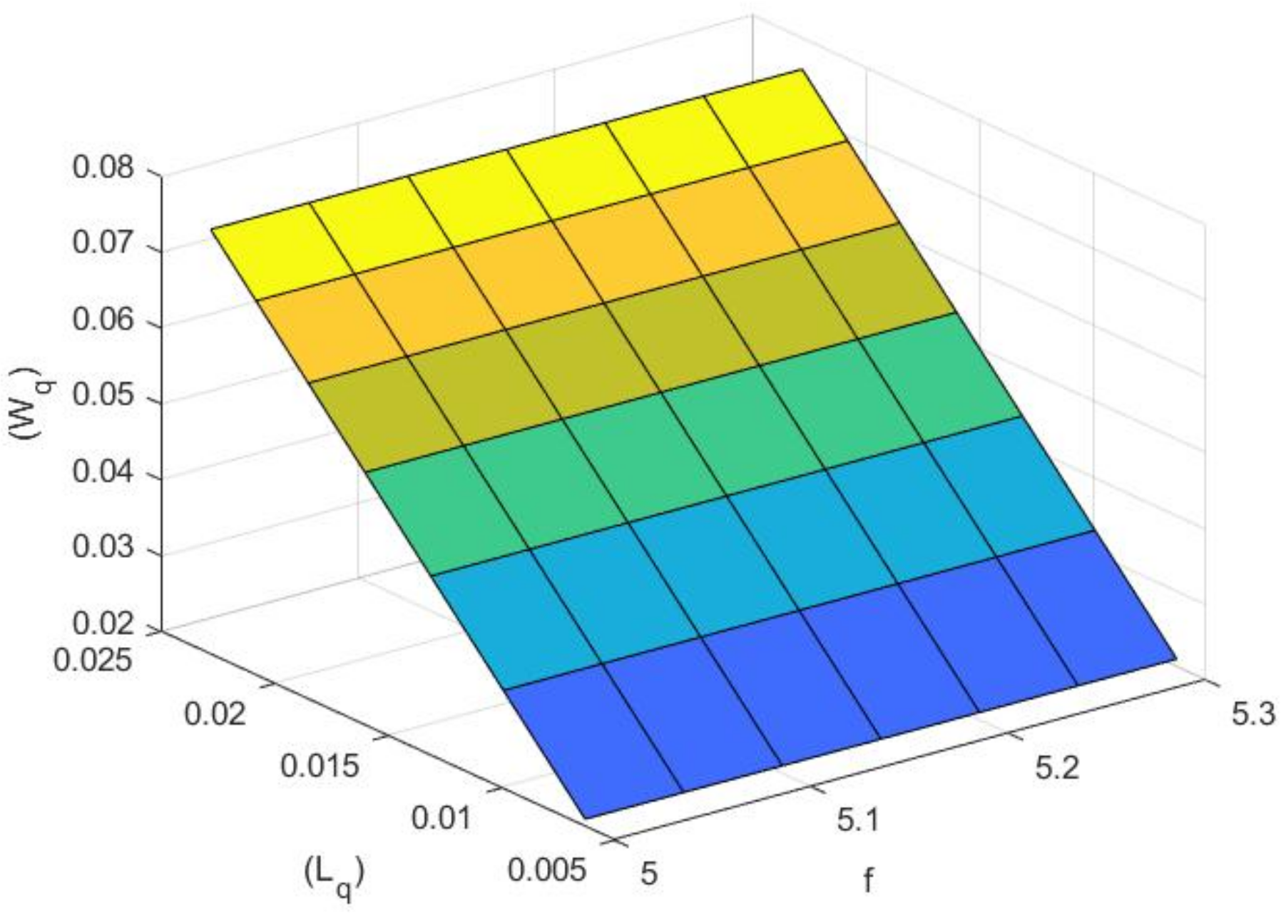
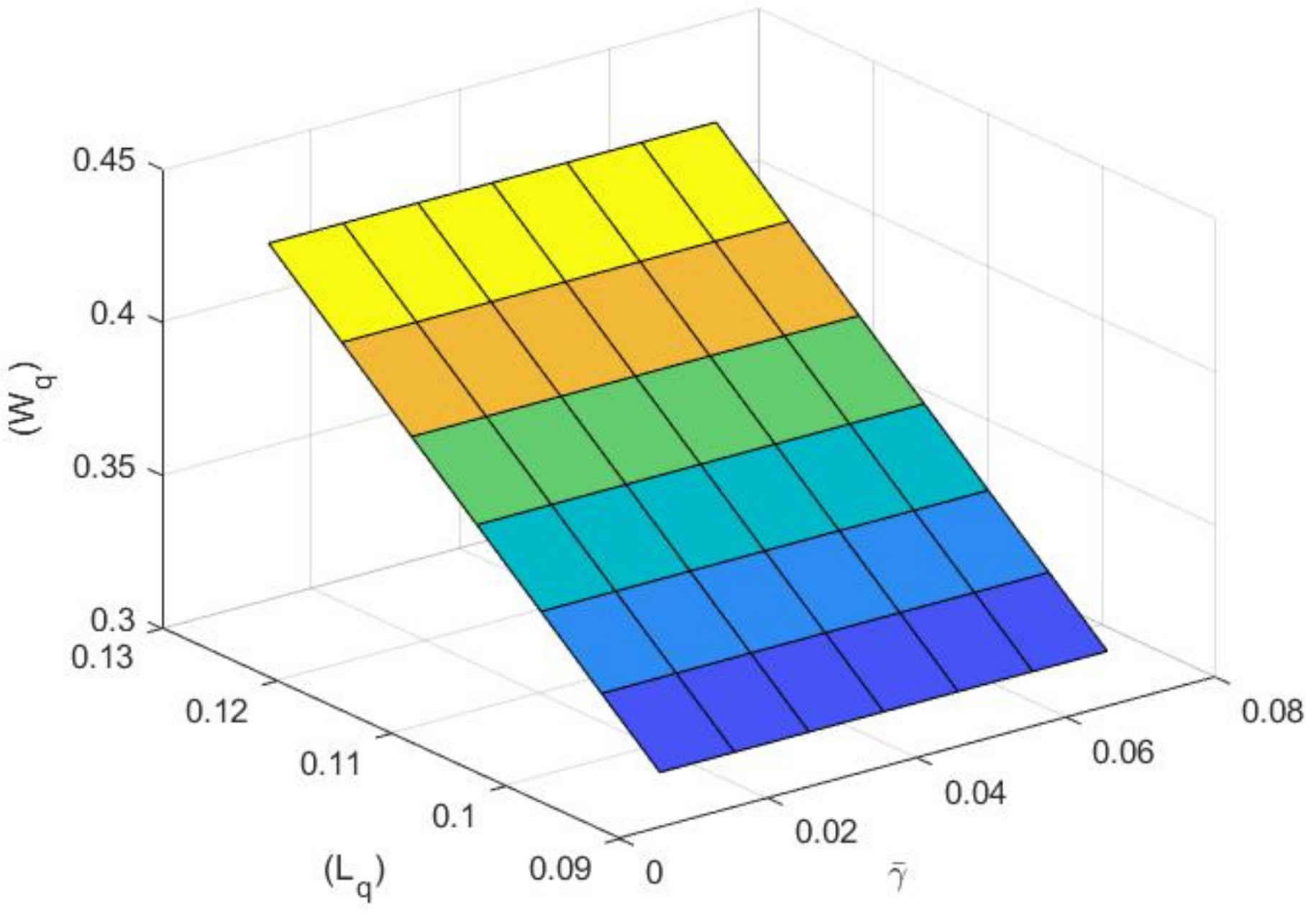
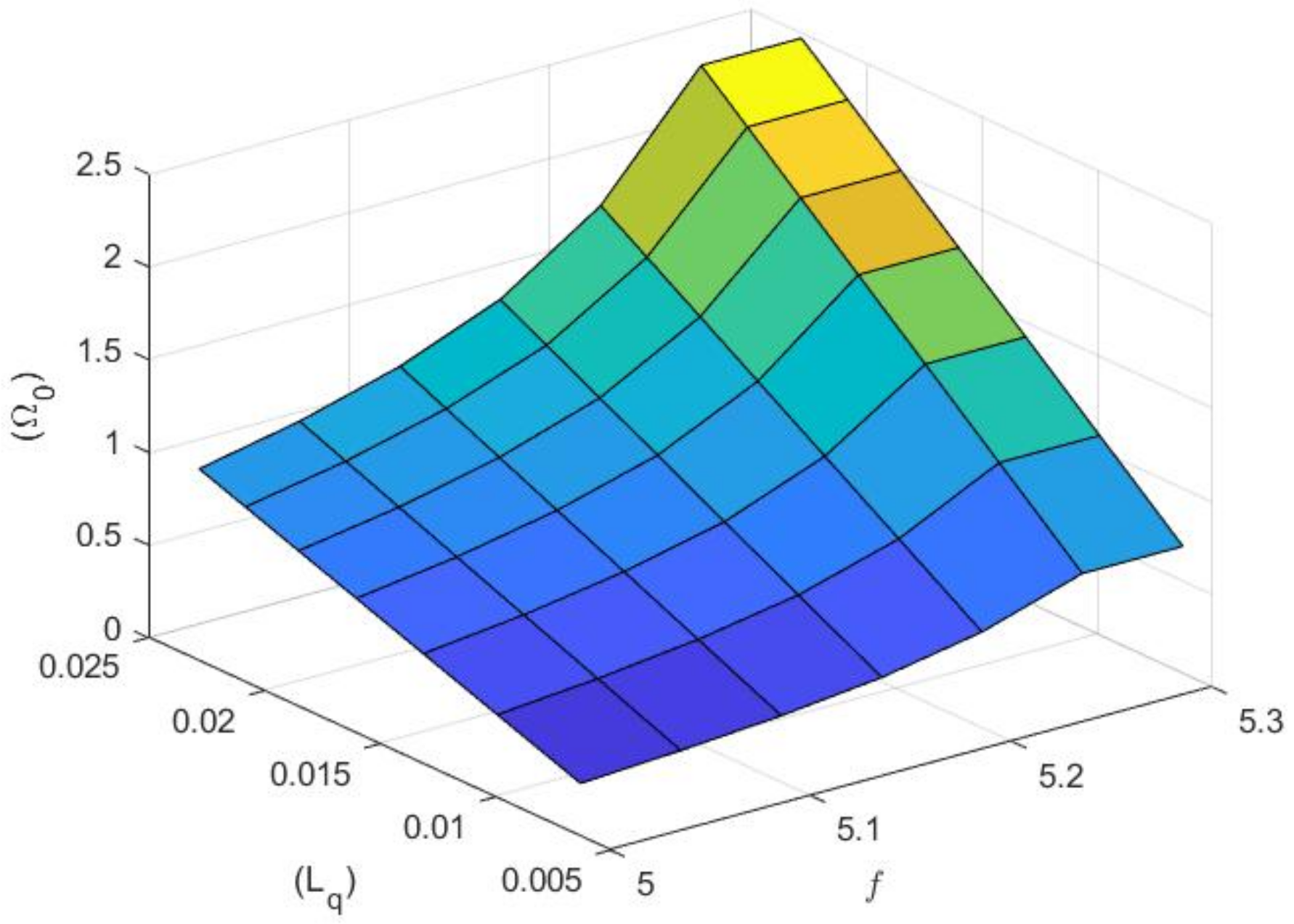
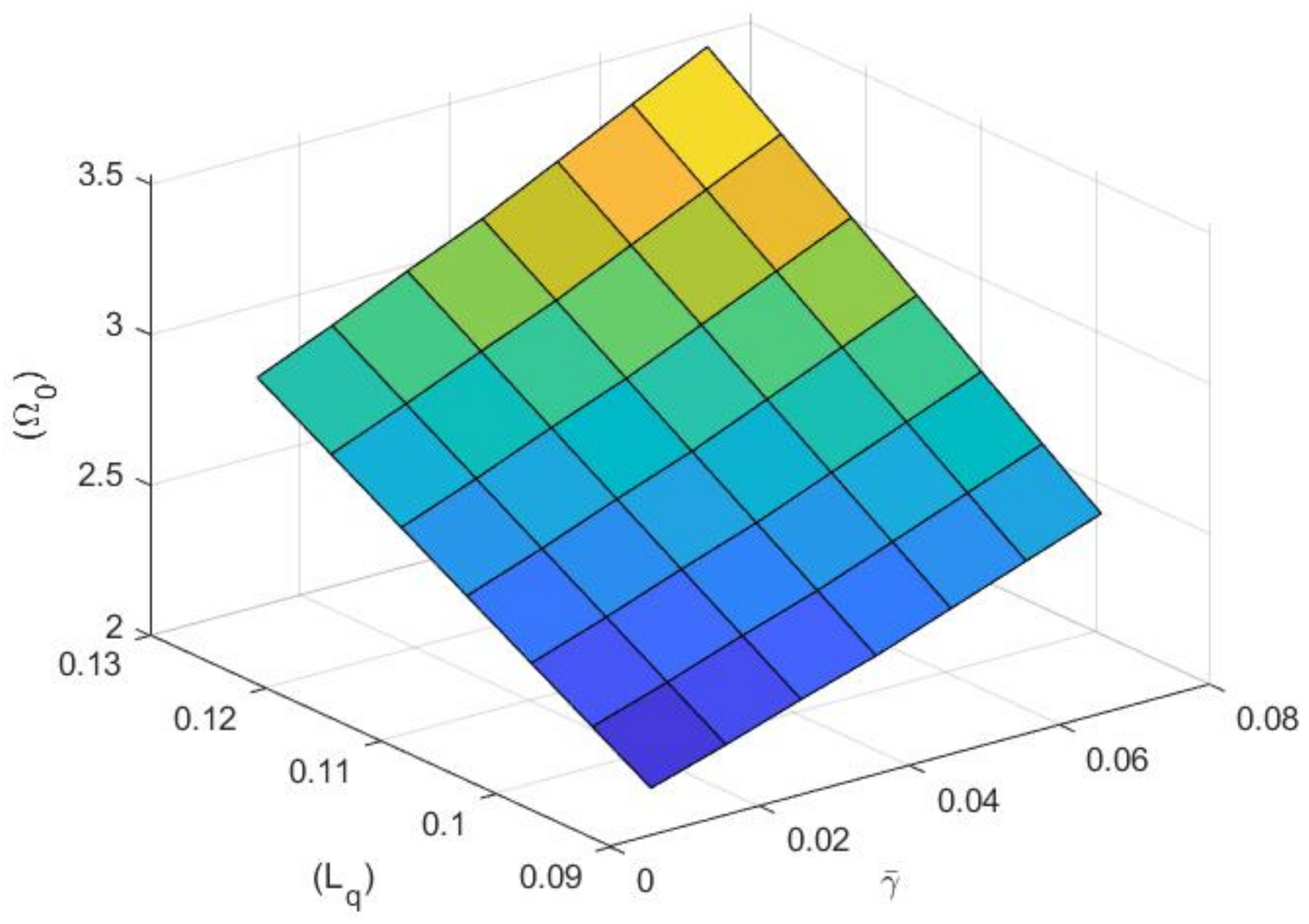
With the effect of the parameters $\alpha ,$ $\beta ,$ $\omega ,$ $\xi ,$ $\overline{\gamma },$ $\eta$, Figure 1, Figure 2, Figure 3 and Figure 4 represents a three-dimensional graph that depict the system’s performance measures. In Figure 1, the surface displays the escalation of the retrial rate $\left(f\right)$, as $\left(L_q\right)$ and $\left(W_q\right)$ decline. In Figure 2, we found that $\left(L_q\right)$ and $\left(W_q\right)$ diminishes, while the feedback rate $\overline{\gamma }$ increases. Figure 3, shows that as ${\mathsf{\Omega }}_0$ and retrial rate f mounts, $\left(L_q\right)$ subsides. Figure 4, shows that as feedback rate $\overline{\gamma }$ mounts, ${\mathsf{\Omega }}_0$ and $\left(L_q\right)$ subsides.

We can identify the effect of characteristics on the system’s evaluation criteria using the numerical results above, and we can be certain that the results are comparable to real-world circumstances.

7. Conclusions

We examined a single-server retrial queue with delayed repair and feedback under working vacations and breakdowns in this article. The system can be stabilised if the necessary and adequate criteria is viable. The PGF of the no. of consumers in the system and its orbit are determined using the PGF approach and supplementary variable approach, whenever it is ideal, normal busy, and on slower pace service. Some numerical results are provided to investigate the impact of system parameters.The novelty of this investigation is the introduction of delaying repair, impatient consumers in the presence of retrial queues with working vacation policy. Moreover, the analytical conclusions that are proved with the aid of numerical examples may be beneficial in various real-world scenarios to construct the outcomes. Furthermore, our model can be observed as a generalised version of numerous queueing models already in existence, each of which has a variety of features and applications.

References

- Artalejo, J.R.; Gómez-Corral, A. Limiting Distribution of the System State. In Retrial Queueing Systems: A Computational Approach; Springer: Berlin/Heidelberg, Germany, 2008; pp. 39–93. [Google Scholar]
- Ke, J.C.; Wu, C.H.; Zhang, Z.G. Recent developments in vacation queueing models: A short survey. Int. J. Oper. Res. 2010, 7, 3–8. [Google Scholar]
- Servi, L.D.; Finn, S.G. M/M/1 queues with working vacations (m/m/1/wv). Perform. Eval. 2002, 50, 41–52. [Google Scholar] [CrossRef]
- Wu, D.A.; Takagi, H. M/G/1 queue with multiple working vacations. Perform. Eval. 2006, 63, 654–681. [Google Scholar] [CrossRef]
- Wang, J.; Li, J. A single server retrial queue with general retrial times and two-phase service. J. Syst. Sci. Complex. 2009, 22, 291–302. [Google Scholar] [CrossRef]
- Arivudainambi, D.; Godhandaraman, P.; Rajadurai, P. Performance analysis of a single server retrial queue with working vacation. Opsearch 2014, 51, 434–462. [Google Scholar] [CrossRef]
- Chandrasekaran, V.; Indhira, K.; Saravanarajan, M.; Rajadurai, P. A survey on working vacation queueing models. Int. J. Pure Appl. Math 2016, 106, 33–41. [Google Scholar]
- Varalakshmi, M.; Chandrasekaran, V.; Saravanarajan, M. A study on M/G/1 retrial G-queue with two phases of service, immediate feedback and working vacations. In Proceedings of the IOP Conference Series: Materials Science and Engineering, Birmingham, UK, 13–15 October 2017; IOP Publishing, 2017; Volume 263, p. 042156. [Google Scholar]
- Revathi, C. Search of arrivals of an M/G/1 retrial queueing system with delayed repair and optional re-service using modified bernoulli vacation. J. Comput. Math. 2022, 6, 200–209. [Google Scholar]
- Rajadurai, P. Sensitivity analysis of an M/G/1 retrial queueing system with disaster under working vacations and working breakdowns. RAIRO-Oper. Res. 2018, 52, 35–54. [Google Scholar] [CrossRef]
- Boualem, M.; Bareche, A.; Cherfaoui, M. Approximate controllability of stochastic bounds of stationary distribution of an M/G/1 queue with repeated attempts and two-phase service. Int. J. Manag. Sci. Eng. Manag. 2019, 14, 79–85. [Google Scholar] [CrossRef]
- Choudhury, G.; Paul, M. A two phase queueing system with Bernoulli feedback. Int. J. Inf. Manag. Sci. 2005, 16, 35. [Google Scholar]
- Rajadurai, P.; Saravanarajan, M.; Chandrasekaran, V.; Indhira, K. An M/(G1, G2)/1 Feedback Retrial Queue with Two Phase Service, Variant Vacation Policy Under Delaying Repair for Impatient Customer. Int. J. Fuzzy Math. Arch. 2015, 6, 45–55. [Google Scholar]
- Rajadurai, P.; Saravanarajan, M.; Chandrasekaran, V. A study on M/G/1 feedback retrial queue with subject to server breakdown and repair under multiple working vacation policy. Alex. Eng. J. 2018, 57, 947–962. [Google Scholar] [CrossRef]
- Ammar, S.I.; Rajadurai, P. Performance analysis of preemptive priority retrial queueing system with disaster under working breakdown services. Symmetry 2019, 11, 419. [Google Scholar] [CrossRef]
- Khan, I.E.; Paramasivam, R. Reduction in Waiting Time in an M/M/1/N Encouraged Arrival Queue with Feedback, Balking and Maintaining of Reneged Customers. Symmetry 2022, 14, 1743. [Google Scholar] [CrossRef]
- Pakes, A.G. Some conditions for ergodicity and recurrence of Markov chains. Oper. Res. 1969, 17, 1058–1061. [Google Scholar] [CrossRef]
- Sennott, L.I.; Humblet, P.A.; Tweedie, R.L. Mean drifts and the non-ergodicity of Markov chains. Oper. Res. 1983, 31, 783–789. [Google Scholar] [CrossRef]
- Gao, S.; Wang, J.; Li, W.W. An M/G/1 retrial queue with general retrial times, working vacations and vacation interruption. Asia-Pac. J. Oper. Res. 2014, 31, 1440006. [Google Scholar] [CrossRef]
- Gómez-Corral, A. Stochastic analysis of a single server retrial queue with general retrial times. Nav. Res. Logist. 1999, 46, 561–581. [Google Scholar] [CrossRef]
- Zhang, M.; Hou, Z. M/G/1 queue with single working vacation. J. Appl. Math. Comput. 2012, 39, 221–234. [Google Scholar] [CrossRef]
Figure 1.
, verses retrial rate f.
Figure 2.
verses feedback rate .
Figure 3.
verses retrial rate f.
Figure 4.