Article

Crossover Dynamics of Rotavirus Disease under Fractional Piecewise Derivative with Vaccination Effects: Simulations with Real Data from Thailand, West Africa, and the US

1
Department of Mathematics, Faculty of Science and Technology, Suratthani Rajabhat University, Surat Thani 84100, Thailand
2
Department of Mathematics, University of Malakand, Chakdara 18800, Khyber Pakhtunkhwa, Pakistan
3
Department of Electricity and Electronics, Institute of Research and Development of Processes, Faculty of Science, Technology University of the Basque Country Campus of Leioa (Bizkaia), 644 Leioa, Spain
4
Department of Computer Science and Mathematics, Lebanese American University, Beirut 1102 2801, Lebanon
5
Department of Mathematics, Art and Science Faculty, Siirt University, 56100 Siirt, Turkey
6
Department of Mathematics, Mathematics Research Center, Near East University, Near East Boulevard, Mersin 10, 99138 Nicosia, Turkey
*
Author to whom correspondence should be addressed.
Symmetry 2022, 14(12), 2641; https://doi.org/10.3390/sym14122641
Submission received: 9 November 2022 / Revised: 28 November 2022 / Accepted: 6 December 2022 / Published: 14 December 2022

Abstract

:
Many diseases are caused by viruses of different symmetrical shapes. Rotavirus particles are approximately 75 nm in diameter. They have icosahedral symmetry and particles that possess two concentric protein shells, or capsids. In this research, using a piecewise derivative framework with singular and non-singular kernels, we investigate the evolution of rotavirus with regard to the effect of vaccination. For the considered model, the existence of a solution of the piecewise rotavirus model is investigated via fixed-point results. The Adam–Bashforth numerical method along with the Newton polynomial is implemented to deduce the numerical solution of the considered model. Various versions of the stability of the solution of the piecewise rotavirus model are presented using the Ulam–Hyres concept and nonlinear analysis. We use MATLAB to perform the numerical simulation for a few fractional orders to study the crossover dynamics and evolution and effect of vaccination on rotavirus disease. To check the validity of the proposed approach, we compared our simulated results with real data from various countries.

1. Introduction

The sickness causes a lot of deaths. The spread of the illness can be stopped using mathematical models. They are effective instruments for predicting the course of the disease [1,2]. Infectious diseases come in a vast variety, a number of which have minimal impact on our health, while others are lethal. Due to the great infectivity of rotavirus, it is regarded as a directly transmitted illness. For almost 40 years, both in developed and developing nations, it has been acknowledged as the primary cause of gastroenteritis and diarrhoea in babies and young children. The main way that rotaviruses spread is by the fecal–oral pathway, which includes intimate contact between people as well as interaction with contaminated environments [3,4]. Unvaccinated children often contract rotavirus between the ages of 6 and 24 months, and almost always before the age of five. Rotavirus infections typically take two days to develop [5]. Around the world, millions of children have the rotavirus. Although rotavirus infections seldom cause fatalities in high-income nations, they nonetheless place a significant strain on medical resources and can result in serious morbidity. The main method of transmission is when the virus enters another person’s mouth through the infected person’s feces [6,7].
Fever, nausea, vomiting, stomach pains, and frequent watery diarrhoea are some of its manifestations, which can persist up to eight days [8,9,10]. There are seven different types of rotavirus, denoted by the letters A through G. Species A, B, and C are the most frequent to infect humans, with A being the most prevalent. Despite the availability of a fast antigen stool test, the recognition of rotavirus infection is frequently established clinically. According to [11,12], the main ways that rotavirus is spread are by the fecal–oral channel; touching infected hands, surfaces, or objects; and perhaps through respiration. About two days pass during the incubation stage [13,14]. Reinfection occurs; however, with every infection, the immunity grows and the severity of subsequent illnesses decreases [15]. Indeed, it was shown in [16] that children who had two naturally occurring rotavirus infections were completely protected against moderate-to-severe diarrhoea as opposed to children who had never had an infection. Additionally, it has been proven that both symptomatic and silent illnesses offer a comparable level of defence [16].
Moreover, other research [17,18] have noted that breastfeeding exclusively might minimize gastrointestinal infections in newborns, as well as good cleanliness, access to the clean and safe water, and sanitation, although these approaches have not been proven yet to be successful. In addition to the aforementioned measures, a cure has been also proposed as a strategy of rotavirus reduction; this involves regular re-hydration therapy [19,20]. Children are given this orally to prevent dehydration from severe diarrhoea and vomiting. In order to avoid fatal and severe rotavirus illness, rotavirus vaccinations have been suggested as being more successful than alternative methods [21,22]. As a result, the WHO issued global suggestions urging all nations, particularly developing ones, to incorporate the vaccination of infants infected with rotavirus into their national immunisation programs. The GAVI Alliance also pledged to support developing nations’ rotavirus vaccinations programs financially.
The most essential tool for examining the epidemiological features of viral diseases is the mathematical model. Regarding the dynamics of the illness, it may offer some insightful information. Several scholars have undertaken various investigations using various studies concerning the modeling and the dynamical study of the rotavirus disease’s transmission. The model of rotavirus infection introduced by Shim et al. in 2006 [23] takes into account the effects of breastfeeding, seasonally, and the potential for control with vaccination. Namawejje et al. [24]’s model of rotavirus disease, which includes three doses of vaccine and therapy and a bilinear incidence rate, was suggested in 2015. A unique mathematical model for rotavirus illness by Omondi et al. [25] that integrates the bilinear incidence rate and vaccination has been developed and extensively investigated. In order to comprehend the dynamics of rotavirus epidemic propagation, Shuaib and Riyapan [26] created and examined the mathematical model shown below, which incorporates breastfeeding and immunisation into consideration.
d S d t = ( 1 ξ ζ ) Λ + ω M + ν V δ I S ( φ + Υ + ζ ) S , d M d t = Λ ξ + φ S ς δ I M ( ω + ψ + ζ ) M , d V d t = Λ ζ + Υ S + ψ M λ δ I V ( ν + ζ ) V , d I d t = δ S I + ϵ δ I M + λ δ I V ( τ + κ + ζ ) I , d R d t = κ I ζ R ,
with
S ( 0 ) = S 0 > 0 , M ( 0 ) = M 0 0 , V ( 0 ) = V 0 0 , I ( 0 ) = I 0 0 , R ( 0 ) = R 0 0 ,
where S ( t ) , M ( t ) , V ( t ) , I ( t ) , and R ( t ) stand for susceptible, breastfeeding, vaccinated, infected, and recovered compartments. The description of the parameter are given in the Table 1.
Fractional-order (FO) models have attracted greater attention from researchers during the last 20 years [27,28]. Compared to traditional integer-order models, they provide novel, accurate, and deeper information on the complicated activity of many diseases [29,30]. Due to genetic characteristics and descriptions memory, classical-order systems are not superior to FO systems. Numerous equations of integer order are used in mathematical models (IDEs). The real events are improved for a higher degree of accuracy and precision using fractional differential equations (FDEs). As a result, Ahmad et al. [31] used the Atangana–Baleanu fractional derivative with the impacts of vaccination and lactation on the FO model of rotavirus outbreaks. Some more applications of fractional calculus can be found in [32,33].
A novel class of operators called piecewise integrals and derivatives was recently presented by Atangana and Araz [34]. Since the timing of the crossover cannot be specified by the exponential or Mittag–Lefler mappings, in order to overcome these challenges, one of the unique methods of piecewise derivatives has been proposed in [34]. The cross-over behaviors using these operators must now be studied in a new way by researchers. Some applications of piecewise fractional operators are available in the literature [35,36,37]. Based on these benefits, we will investigate the model (1) using the piecewise Caputo and Atangana–Baleanu operator in the manner as follows:
0 P C A B C D t m S ( t ) = ( 1 ξ ζ ) Λ + ω M + ν V δ I S ( φ + Υ + ζ ) S , 0 P C A B C D t m M ( t ) = Λ ξ + φ S ς δ I M ( ω + ψ + ζ ) M , 0 P C A B C D t m V ( t ) = Λ ζ + Υ S + ψ M λ δ I V ( ν + ζ ) V , 0 P C A B C D t m I ( t ) = δ S I + ϵ δ I M + λ δ I V ( τ + κ + ζ ) I , 0 P C A B C D t m R ( t ) = κ I ζ R .
More specifically, we can write Equation (2) as
0 C A B C D t m ( S ( t ) ) = 0 C D t m ( S ( t ) ) = C ϝ 1 ( S , t ) , 0 < t t 1 , 0 A B C D t m ( S ( t ) ) = A B C ϝ 1 ( S , t ) , t 1 < t T , 0 C A B C D t m ( M ( t ) ) = 0 C D t m ( M ( t ) ) = C ϝ 2 ( M , t ) , 0 < t t 1 , 0 A B C D t m ( M ( t ) ) = A B C ϝ 2 ( M , t ) , t 1 < t T , 0 C A B C D t m ( V ( t ) ) = 0 C D t m ( V ( t ) ) = C ϝ 3 ( V , t ) , 0 < t t 1 , 0 A B C D t m ( V ( t ) ) = A B C ϝ 3 ( V , t ) , t 1 < t T , 0 C A B C D t m ( I ( t ) ) = 0 C D t m ( I ( t ) ) = C ϝ 4 ( I , t ) , 0 < t t 1 , 0 A B C D t m ( I ( t ) ) = A B C ϝ 4 ( I , t ) , t 1 < t T , 0 C A B C D t m ( R ( t ) ) = 0 C D t m ( R ( t ) ) = C ϝ 5 ( R , t ) , 0 < t t 1 , 0 A B C D t m ( R ( t ) ) = A B C ϝ 5 ( R , t ) , t 1 < t T .
In this paper, the epidemic model of rotavirus is investigated under the piecewise fractional operator in the sense of the Caputo and ABC operators. The existence and uniqueness of the solution is derived with the help of fixed point theorems. The Ulam–Hyres-type stability of the solution and its different version is studied through nonlinear functional analysis. The numerical results are derived by using the Adams–Bashforth method. All of the results are validated through numerical simulations with real data from three different countries. The rest of the paper is organized as follows: Section 2 provides the basic notions of the piecewise fractional operators. Section 3 is devoted to the existence and uniqueness of the solution. The results of Ulam–Hyres stability are discussed in Section 4. The numerical results of the proposed model are given Section 5. Numerical simulations of the considered model are provided in Section 6. Section 7 provides the conclusion of the manuscript.

2. Preliminaries

Here, we present some definitions regarding Caputo and A B C fractional, as well as piecewise derivatives and integrals.
Definition 1.
The definition of A B C operator of function M ( t ) with condition M ( t ) H 1 ( 0 , T ) is:
A B C 0 D t m ( M ( t ) ) = A B C ( m ) 1 m 0 t d d P M ( P ) E m m t P m 1 m d P .
Here, ABC ( m ) denotes the normalization function such that A B C ( 0 ) = A B C ( 1 ) = 1 . Additionally, E m is the special function known as Mittag–Leffler function.
Definition 2.
The integral for the ABC operator is expressed by:
A B C 0 I t m M ( t ) = 1 m A B C ( m ) M ( t ) + m A B C ( m ) Γ ( m ) 0 t M ( P ) ( t P ) m 1 d P .
Definition 3.
The Caputo operator for a function M ( t ) is defined as
0 C D t m M ( t ) = 1 Γ ( 1 m ) 0 t d d P M ( P ) ( t P ) m d P .
Definition 4.
Suppose M ( t ) is piecewise differentiable; then, the piecewise derivative with the Caputo and ABC operators [17] is
0 P C A B C D t m M ( t ) = 0 C D t m M ( t ) , 0 < t t 1 , 0 A B C D t m M ( t ) t 1 < t T ,
here, 0 P C A B C D t m represents a piecewise differential operator, where the Caputo operator is in the interval 0 < t t 1 and the A B C operator is in the interval t 1 < t T .
Definition 5.
Suppose M ( t ) is a piecewise integrable; then, the piecewise integral with Caputo and ABC operators [17] is
0 P C A B C I t M ( t ) = 1 Γ ( m ) t 1 t M ( P ) ( t P ) m 1 d ( P ) , 0 < t t 1 , 1 m A B C ( m ) M ( t ) + m A B C ( m ) Γ ( m ) t 1 t M ( P ) ( t P ) m 1 d ( P ) t 1 < t T , ,
here, 0 P C A B C I t m represents the piecewise integral operator, where the Caputo operator is in interval 0 < t t 1 and the A B C operator in interval t 1 < t T .

3. Existence and Uniqueness

The existence and the uniqueness results of the suggested model in the piecewise notion are found in this part. We shall now determine whether a solution exists for the hypothetical piecewise derivable function as well as its specific solution attribute. In order to do this, we can also write the following by way of more explanation.
0 P C A B C D t m Q ( t ) = W ( t , Q ( t ) ) , 0 < m 1 ,
is
Q ( t ) = Q 0 + 1 Γ ( m ) 0 t W ( ϑ , Q ( ϑ ) ) ( t ϑ ) m 1 d ϑ , 0 < t t 1 , Q ( t 1 ) + 1 m A B C ( m ) W ( t , Q ( t ) ) + m A B C ( m ) Γ ( m ) t 1 t ( t ϑ ) m 1 W ( ϑ , Q ( ϑ ) ) d ( ϑ ) , t 1 < t T ,
where
Q ( t ) = S ( t ) M ( t ) V ( t ) I ( t ) R ( t ) , Q 0 = S 0 M 0 V 0 I 0 R 0 , Q ( t 1 ) = S ( t 1 ) M ( t 1 ) V ( t 1 ) I ( t 1 ) R ( t 1 ) , W ( t , Q ( t ) ) = ϝ 1 = C ϝ 1 ( S , t ) A B C ϝ 1 ( S , t ) , ϝ 2 = C ϝ 2 ( M , t ) A B C ϝ 2 ( M , t ) , ϝ 3 = C ϝ 3 ( V , t ) A B C ϝ 3 ( V , t ) , ϝ 4 = C ϝ 4 ( I , t ) A B C ϝ 4 ( I , t ) , ϝ 5 = C ϝ 5 ( R , t ) A B C ϝ 5 ( R , t ) .
Taking 0 < t T < and the Banach space E 1 = C [ 0 , T ] with a norm
Q = max t [ 0 , T ] | Q ( t ) | .
We assume the following growth condition:
(C1) 
L Q > 0 ; ∀ W , Q ¯ E we have
| W ( t , Q ) W ( t , Q ¯ ) | m a t h c a l L W | Q Q ¯ | .
(C2) 
C W > 0 & M W > 0 , ;
| W ( t , Q ( t ) ) | C W | Q | + M W .
Theorem 1.
If W be piece-wise continuous on ( 0 , t 1 ] and [ t 1 , T ] on [ 0 , T ] , also satisfy ( C 2 ) ; then, (3) has least one solution.
Proof. 
Let us define a closed sub-set as B and E in both subintervals of [ 0 , L ] .
B = { Q E : Q R 1 , 2 , R > 0 } ,
Suppose L : B B and using (6) as
L ( Q ) = Q 0 + 1 Γ ( m ) 0 t 1 W ( ϑ , Q ( ϑ ) ) ( t ϑ ) m 1 d ϑ , 0 < t t 1 , Q ( t 1 ) + 1 m A B C ( m ) W ( t , Q ( t ) ) + m A B C ( m ) Γ ( m ) t 1 t ( t ϑ ) m 1 W ( ϑ , Q ( ϑ ) ) d ( ϑ ) , t 1 < t T ,
For any Q B , we have
| L ( Q ) ( t ) | | Q 0 | + 1 Γ ( m ) 0 t 1 ( t ϑ ) m 1 | W ( ϑ , Q ( ϑ ) ) | d ϑ , | Q ( t 1 ) | + 1 m A B C ( m ) | W ( t , Q ( t ) ) | + m A B C ( m ) Γ ( m ) t 1 t ( t ϑ ) m 1 | W ( ϑ , Q ( ϑ ) ) | d ( ϑ ) , | Q 0 | + 1 Γ ( m ) 0 t 1 ( t ϑ ) m 1 [ C W | Q | + M W ] d m , | Q ( t 1 ) | + 1 m A B C ( m ) [ C W | Q | + M W ] + m A B C ( m ) Γ ( m ) t 1 t ( t ϑ ) m 1 [ C W | Q | + M W ] d ( m ) , | Q 0 | + T m Γ ( m + 1 ) [ C H | Q | + M W ] = R 1 , 0 < t t 1 , | Q ( t 1 ) | + 1 m A B C ( m ) [ C W | Q | + M W ] + m ( T T ) m A B C ( m ) Γ ( m ) + 1 [ C W | Q | + M W ] d ( m ) = R 2 , t 1 < t T , R 1 , 0 < t t 1 , R 2 , t 1 < t T .
As determined by the previous equation, Q B . Therefore, L ( B ) B . Thus, it demonstrates that L is closed and complete. In order to further demonstrate the completely continuity, we may present t i < t j [ 0 , t 1 ] as an initial interval in the sense of Caputo. Consider the following:
| L ( Q ) ( t j ) L ( Q ) ( t i ) | = | 1 Γ ( m ) 0 t j ( t j ϑ ) m 1 W ( ϑ , Q ( ϑ ) ) d ϑ 1 Γ ( m ) 0 t i ( t i ϑ ) m 1 W ( ϑ , Q ( ϑ ) ) d ϑ | 1 Γ ( m ) 0 t i [ ( t i ϑ ) m 1 ( t j ϑ ) m 1 ] | W ( ϑ , Q ( ϑ ) ) | d ϑ + 1 Γ ( m ) t i t j ( t j ϑ ) m 1 | W ( ϑ , Q ( ϑ ) ) | d ϑ 1 Γ ( m ) [ 0 t i [ ( t i ϑ ) m 1 ( t j ϑ ) m 1 ] d ϑ + t i t j ( t j ϑ ) m 1 d ϑ ] ( C H | Q | + M W ) ( C W Q + M W ) Γ ( m + 1 ) [ t j ϑ t i m + 2 ( t j t i ) m ] .
If t i t j , then
| L ( Q ) ( t j ) L ( Q ) ( t i ) | 0 , as t i t j .
So, L is equicontinuous in [ 0 , t 1 ] . Consider t i , t j [ t 1 , T ] in the A B C sense as
| L ( Q ) ( t j ) L ( Q ) ( t i ) | = | 1 m A B C ( m ) W ( t , Q ( t ) ) + m A B C ( m ) Γ ( m ) t 1 t j ( t j ϑ ) m 1 W ( ϑ , Q ( ϑ ) ) d ϑ 1 m A B C ( m ) W ( t , Q ( t ) ) + ( m ) A B C ( m ) Γ ( m ) t 1 t i ( t i ϑ ) m 1 W ( ϑ , Q ( ϑ ) ) d ϑ | m A B C ( m ) Γ ( m ) t 1 t i [ ( t i ϑ ) m 1 ( t j ϑ ) m 1 ] | W ( ϑ , Q ( ϑ ) ) | d ϑ + m A B C ( m ) Γ ( m ) t i t j ( t j ϑ ) m 1 | W ( ϑ , Q ( ϑ ) ) | d ϑ m A B C ( m ) Γ ( m ) [ t 1 t i [ ( t i ϑ ) m 1 ( t j ϑ ) m 1 ] d ϑ + t i t j ( t j ϑ ) m 1 d m ] ( C W | Q | + M W ) m ( C W Q + M W ) A B C ( m ) Γ ( m + 1 ) [ t j m t i m + 2 ( t j t i ) m ] .
If t i t j , then
| L ( Q ) ( t j ) L ( Q ) ( t i ) | 0 , as t i t j .
So, L , which shows its equi-continuity in [ t 1 , T ] . Thus, L is an equi-continuous map. Based on the Arzel’a–Ascoli result, L is continuous (completely), uniformly continuous, and bounded as the Schauder result indicates that problem (3) contains the solution to at least one solution in the subintervals.
Further, if L is a contraction mapping with ( C 1 ) , then the suggested system has a unique solution. Since L : B B is a piece-wise continuous operator, consider Q and Q ¯ B on [ 0 , t 1 ] in the sense of Caputo as
L ( Q ) L ( Q ¯ ) = max t [ 0 , t 1 ] | 1 Γ ( m ) 0 t ( t ϑ ) m 1 W ( ϑ , Q ( ϑ ) ) d ϑ 1 Γ ( m ) 0 t ( t ϑ ) m 1 W ( ϑ , W ¯ ( ϑ ) ) d ϑ | T m Γ ( m + 1 ) L W Q Q ¯ .
From (11), we have
L ( Q ) L ( Q ¯ ) T m Γ ( m + 1 ) L W Q Q ¯ .
As a result, L is a contraction. So, the model under consideration has a only one solution in the provided sub interval in light of the Banach contraction result. Additionally, t [ t 1 , T ] in the sense of the A B C derivative as
L ( Q ) L ( Q ¯ ) 1 m A B C ( m ) L W Q Q ¯ + m ( T T m ) A B C ( m ) Γ ( m + 1 ) L ϝ Q Q ¯ .
or
L ( Q ) L ( Q ¯ ) L W 1 m A B C ( m ) + m ( T T ) m A B C ( m ) Γ ( m + 1 ) Q Q ¯ .
Thus, L is a contraction. As a result, the model under consideration has a unique solution in the provided sub interval in light of the Banach contraction result. Hence, the proof is finished. □

4. Stability Analysis

In this portion, we demonstrate the H-U stabilities of the solution of the model (2).
Definition 6.
The PW rotavirus model (2) is U-H-stable, if for each d > 0 , we have:
P C A B C D t m Θ ( t ) ϝ ( t , Θ ( t ) ) < d , f o r a l l , t T ,
and ∃ H > 0 and a unique solution Θ ¯ Z such that,
Θ Θ ¯ Z H d , f o r a l l , t T .
Moreover, if a non-decreasing function K : [ 0 , ) R + , then
Θ Θ ¯ Z H K ( d ) , a t e v e r y , t T ,
with K ( 0 ) = 0 , then acquired solution is generalized U-H-stable.
Definition 7.
The model (2) is H-U-R-stable if G : [ 0 , ) R + , for each d > 0 , and inequality
P C A B C D t m Θ ( t ) ϝ ( t , Θ ( t ) ) < d G ( t ) , f o r a l l , t T ,
H G > 0 and a unique solution Θ ¯ Z , so that
Θ Θ ¯ Z H G d G ( t ) , t T .
Let G : [ 0 , ) R + , so that
P C A B C D t m Θ ( t ) ϝ ( t , Θ ( t ) ) < G ( t ) , t T ,
H G > 0 and a unique solution Θ ¯ Z , so that
Θ Θ ¯ Z H G G ( t ) , t T .
the acquired solution is generalized H-U-R-stable.
Remark 1.
Consider a function ϕ 1 C ( T ) so that it does not on Θ Z , and ϕ 1 ( 0 ) = 0 , and
ϕ 1 ( t ) d , t T ; P C A B C D t m Θ ( t ) = ϝ t , Θ ( t ) + ϕ 1 ( t ) , t T .
Lemma 1.
Consider the system as:
0 P C A B C D t ϱ Θ ( t ) = ϝ ( t , Θ ( t ) ) , 0 < ϱ 1 .
One can get the solution of the system (22) as
Θ ( t ) = Θ 0 + 1 Γ ( m ) 0 t ϝ ( ϱ , Θ ( ϱ ) ) ( t ϱ ) m 1 d ϱ , 0 < t t 1 Θ ( t 1 ) + 1 m A B C ( m ) ϝ ( t , Θ ( t ) ) + m A B C ( m ) Γ ( m ) t 1 t ( t ϱ ) m 1 ϝ ( ϱ , Θ ( ϱ ) ) d ( ϱ ) , t 1 < t T ,
and
F ( Θ ) F ( Θ ¯ ) T 1 m Γ ( m + 1 ) d t T 1 , ( 1 m ) Γ ( m ) + ( T 2 m ) A B C ( m ) Γ ( m ) d = Λ d , t T 2 .
Theorem 2.
In light of Lemma (1) if the condition L f T m Γ ( m ) < 1 holds, then the solution of the PW rotavirus model (2) is H-U as well as generalized H-U-stable.
Proof. 
Let Θ Z satisfy the Equation (2) and Θ ¯ Z be a unique solution of (2); so, we have two parts:
Case:1 For t T , we consider the Caputo case. Consider
Θ Θ ¯ = sup t T Θ Θ + 1 Γ ( m ) 0 t 1 ( t 1 s ) m 1 ϝ s , Θ ¯ ( s ) d s
sup t T Θ Θ + 1 Γ ( m ) 0 t 1 ( t 1 s ) m 1 ϝ s , Θ ¯ ( s ) d s
+ sup t T + 1 Γ ( m ) 0 t 1 ( t 1 s ) m 1 ϝ s , Θ ( s ) d s
1 Γ ( m ) 0 t 1 ( t 1 s ) m 1 ϝ s , Θ ¯ ( s ) d s
T 1 m Γ ( m + 1 ) d + L f T 1 Γ ( m + 1 ) Θ Θ ¯ .
Through further simplification
Θ Θ ¯ T 1 Γ ( m + 1 ) 1 L f T 1 Γ ( m + 1 ) d .
Case:2
Θ Θ ¯ sup t T Θ Θ ( t 1 ) + 1 m A B C ( m ) ϝ t , Θ ( t ) + m A B C ( m ) Γ ( m ) t 1 t ( t s ) m 1 ϝ s , Θ ¯ ( s ) d ( s ) + sup t T 1 m A B C ( m ) ϝ t , Θ ( t ) ϝ t , Θ ¯ ( t ) + sup t T m A B C ( m ) Γ ( m ) t 1 t ( t s ) m 1 ϝ s , Θ ( s ) ϝ s , Θ ¯ ( s ) d s .
Through further simplification and using Λ = ( 1 m ) Γ ( m ) + T 2 m A B C ( m ) Γ ( m ) , we have
Θ Θ ¯ Z Λ d + Λ L f Θ Θ ¯ Z ,
we have
Θ Θ ¯ Z Λ 1 Λ L f d Θ Θ ¯ Z .
Using
H = max T 1 Γ ( m + 1 ) 1 L f T 1 Γ ( m + 1 ) , Λ 1 Λ L f 1 M f .
Now from Equations (30) and (34), we have
Θ Θ ¯ Z H d , a t e a c h t T .
Hence, the solution of the PW rotavirus model (2) is H-U-stable. Moreover, by replacing d with K ( d ) , we have
Θ Θ ¯ Z H K ( d ) , a t e a c h t T .
Thus, the solution of the PW rotavirus model (2) is G-H-U-stable. □
Remark 2.
Consider ϕ 1 C ( T ) with ϕ 1 ( 0 ) = 0 ; then,
ϕ 1 ( t ) G ( t ) d , t T ; P C A B C D t m Θ ( t ) = ϝ t , Θ ( t ) + ϕ 1 ( t ) , t T .
Lemma 2.
Solution to the model
P C A B C D t m Θ ( t ) = ϝ t , Θ ( t ) + ϕ 1 ( t ) , Θ ( 0 ) = Θ ,
satisfies the following inequality:
F ( Θ ) F ( Θ ¯ ) T 1 m Γ ( m + 1 ) C G G ( t ) d , t T 1 , ( 1 m ) Γ ( m ) + ( T 2 m ) A B C ( m ) Γ ( m ) C G G ( t ) d = Λ C G G ( t ) d , t T 2 .
where H f , G , Λ = Λ H f , G .
Remark 2 can be used to obtain Equation (31).
Theorem 3.
The solution of the PW rotavirus model is H-U-R-stable if the following conditions hold:
(H1) For each Θ , v Z and a constant C K > 0 , we obtain
K ( Θ ) K ( v ) C K Θ v ;
(H2) For each Θ , v , Θ ¯ , v ¯ Z and constant L f > 0 , 0 < M f < 1 , we obtain
ϝ ( t , Θ , v ) ϝ ( t , Θ ¯ , v ¯ ) L f Θ Θ ¯ + M f v v ¯ .
Proof. 
We prove the results in two parts.
Case:1 for t T , we have
Θ Θ ¯ = sup t T Θ Θ + 1 Γ ( m ) 0 t 1 ( t 1 s ) m 1 ϝ s , Θ ¯ ( s ) d s sup t T Θ Θ + 1 Γ ( m ) 0 t 1 ( t 1 s ) m 1 ϝ s , Θ ¯ ( s ) d s + sup t T + 1 Γ ( m ) 0 t 1 ( t 1 s ) m 1 ϝ s , Θ ( s ) d s 1 Γ ( m ) 0 t 1 ( t 1 s ) m 1 ϝ s , Θ ¯ ( s ) d s T 1 m Γ ( m + 1 ) C K K ( t ) d + L f T 1 Γ ( m + 1 ) Θ Θ ¯ .
Through further simplification
Θ Θ ¯ C K K ( t ) T 1 Γ ( m + 1 ) 1 L f T 1 Γ ( m + 1 ) d .
Case:2
Θ Θ ¯ sup t T Θ Θ ( t 1 ) + 1 m A B C ( m ) ϝ t , Θ ( t ) + m A B C ( m ) Γ ( m ) t 1 t ( t s ) m 1 ϝ s , Θ ¯ ( s ) d ( s ) + sup t T 1 m A B C ( m ) ϝ t , Θ ( t ) ϝ t , Θ ¯ ( t ) + sup t T m A B C ( m ) Γ ( m ) t 1 t ( t s ) m 1 ϝ s , Θ ( s ) ϝ s , Θ ¯ ( s ) d s .
Through further simplification and using Λ = ( 1 m ) Γ ( m ) + T 2 m A B C ( m ) Γ ( m ) , we have
Θ Θ ¯ Z Λ C K K ( t ) d + Λ L f Θ Θ ¯ Z ,
we have
Θ Θ ¯ Z Λ C K K ( t ) 1 Λ L f d Θ Θ ¯ Z .
Using
H Λ , C K = max T 1 Γ ( m + 1 ) 1 L f T 1 Γ ( m + 1 ) , C K K ( t ) Λ 1 Λ L f 1 M f .
Now, from Equations (30) and (34), we have
Θ Θ ¯ Z H Λ , C K d , a t e a c h t T .
Hence, the theorem is proved. □
Remark 3.
Let ϕ 1 C ( T ) with ϕ 1 ( 0 ) = 0 ; then,
ϕ 1 ( t ) G ( t ) , t T .
Theorem 4.
Using H 1 , H 2 , and Remarks 2 and 3, the solution of the PW rotavirus model (2) is generalized H-U-R-stable, if M f < 1 .
Where
(H1) For each Θ , v Z and constant C K > 0 , we obtain
K ( Θ ) K ( v ) C K Θ v ;
and
(H2) For each Θ , v , Θ ¯ , v ¯ Z and constant L f > 0 , 0 < M f < 1 , we obtain
ϝ ( t , Θ , v ) ϝ ( t , Θ ¯ , v ¯ ) L f Θ Θ ¯ + M f v v ¯ .
Proof. 
We obtain our results in two parts:
Case:1 We consider the Caputo operator in the t T . Consider
Θ Θ ¯ = sup t T Θ Θ + 1 Γ ( m ) 0 t 1 ( t 1 s ) m 1 ϝ s , Θ ¯ ( s ) d s sup t T Θ Θ + 1 Γ ( m ) 0 t 1 ( t 1 s ) m 1 ϝ s , Θ ¯ ( s ) d s + sup t T + 1 Γ ( m ) 0 t 1 ( t 1 s ) m 1 ϝ s , Θ ( s ) d s 1 Γ ( m ) 0 t 1 ( t 1 s ) m 1 ϝ s , Θ ¯ ( s ) d s T 1 m Γ ( m + 1 ) C K K ( t ) d + L f T 1 Γ ( m + 1 ) Θ Θ ¯ .
Through further simplification
Θ Θ ¯ C K K ( t ) T 1 Γ ( m + 1 ) 1 L f T 1 Γ ( m + 1 ) d .
Case:2
Θ Θ ¯ sup t T Θ Θ ( t 1 ) + 1 m A B C ( m ) ϝ t , Θ ( t ) + m A B C ( m ) Γ ( m ) t 1 t ( t s ) m 1 ϝ s , Θ ¯ ( s ) d ( s ) + sup t T 1 m A B C ( m ) ϝ t , Θ ( t ) ϝ t , Θ ¯ ( t ) + sup t T m A B C ( m ) Γ ( m ) t 1 t ( t s ) m 1 ϝ s , Θ ( s ) ϝ s , Θ ¯ ( s ) d s .
Through further simplification and using Λ = ( 1 m ) Γ ( m ) + T 2 m A B C ( m ) Γ ( m ) , we have
Θ Θ ¯ Z Λ C K K ( t ) d + Λ L f Θ Θ ¯ Z ,
we have
Θ Θ ¯ Z Λ C K K ( t ) 1 Λ L f Θ Θ ¯ Z .
Using
H Λ , C K = max T 1 Γ ( m + 1 ) 1 L f T 1 Γ ( m + 1 ) , C K K ( t ) Λ 1 Λ L f .
Now, from Equations (30) and (34), we have
Θ Θ ¯ Z H Λ , C K , a t e a c h t T .
The generalized H-U-R stability of the solution is proved. □

5. Numerical Scheme for the Fractional Piecewise Rotavirus Model

In this section, we derive the numerical scheme for the following rotavirus epidemic model (2):
0 P C A B C D t m S ( t ) = ( 1 ξ ζ ) Λ + ω M + ν V δ I S ( φ + Υ + ζ ) S , 0 P C A B C D t m M ( t ) = Λ ξ + φ S ς δ I M ( ω + ψ + ζ ) M , 0 P C A B C D t m V ( t ) = Λ ζ + Υ S + ψ M λ δ I V ( ν + ζ ) V , 0 P C A B C D t m I ( t ) = δ S I + ϵ δ I M + λ δ I V ( τ + κ + ζ ) I , 0 P C A B C D t m R ( t ) = κ I ζ R .
By applying the piece-wise integral to the Caputo and AB derivative, we obtain
S ( t ) = S ( 0 ) + 1 Γ ( m ) 0 t 1 ( t ρ ) m 1 c ϝ 1 ( t , S ) d ρ 0 < t t 1 , S ( t 1 ) + 1 m A B ( m ) ϝ 1 ( t , S ) d ρ + m A B ( m ) Γ ( m ) t 1 t ( t ρ ) m 1 ϝ 1 ( t , S ) d ρ t 1 < t T , M ( t ) = M ( 0 ) + 1 Γ ( m ) 0 t 1 ( t ρ ) m 1 c ϝ 2 ( t , M ) d ρ 0 < t t 1 , M ( t 1 ) + 1 m A B ( m ) ϝ 2 ( t , M ) d ρ + m A B ( m ) Γ ( m ) t 1 t ( t ρ ) m 1 ϝ 2 ( t , M ) d ρ t 1 < t T , V ( t ) = V ( 0 ) + 1 Γ ( m ) 0 t 1 ( t ρ ) m 1 c ϝ 3 ( t , V ) d ρ 0 < t t 1 , V ( t 1 ) + 1 m A B ( m ) ϝ 3 ( t , V ) d ρ + m A B ( m ) Γ ( m ) t 1 t ( t ρ ) m 1 ϝ 3 ( t , V ) d ρ t 1 < t T , I ( t ) = I ( 0 ) + 1 Γ ( m ) 0 t 1 ( t ρ ) m 1 c ϝ 4 ( t , I ) d ρ 0 < t t 1 , I ( t 1 ) + 1 m A B ( m ) ϝ 4 ( t , I ) d ρ + m A B ( m ) Γ ( m ) t 1 t ( t ρ ) m 1 ϝ 4 ( t , I , ) d ρ t 1 < t T , R ( t ) = R ( 0 ) + 1 Γ ( m ) 0 t 1 ( t ρ ) m 1 c ϝ 5 ( t , R ) d ρ 0 < t t 1 , R ( t 1 ) + 1 m A B ( m ) ϝ 5 ( t , R ) d ρ + m A B ( m ) Γ ( m ) t 1 t ( t ρ ) m 1 ϝ 5 ( t , R ) d ρ t 1 < t T ,
At t = t n + 1
S ( t ) = S ( 0 ) + 1 Γ ( m ) 0 t 1 ( t ρ ) m 1 c ϝ 1 ( t , S ) d ρ 0 < t t 1 , S ( t 1 ) + 1 m A B ( m ) ϝ 1 ( t , S ) d ρ + m A B ( m ) Γ ( m ) t 1 t n + 1 ( t ρ ) m 1 ϝ 1 ( t , S ) d ρ t 1 < t T , M ( t ) = M ( 0 ) + 1 Γ ( m ) 0 t 1 ( t ρ ) m 1 c ϝ 2 ( t , M ) d ρ 0 < t t 1 , M ( t 1 ) + 1 m A B ( m ) ϝ 2 ( t , M ) d ρ + m A B ( m ) Γ ( m ) t 1 t n + 1 ( t ρ ) m 1 ϝ 2 ( t , M ) d ρ t 1 < t T , V ( t ) = V ( 0 ) + 1 Γ ( m ) 0 t 1 ( t ρ ) m 1 c ϝ 3 ( t , V ) d ρ 0 < t t 1 , V ( t 1 ) + 1 m A B ( m ) ϝ 3 ( t , V ) d ρ + m A B ( m ) Γ ( m ) t 1 t n + 1 ( t ρ ) m 1 ϝ 3 ( t , V ) d ρ t 1 < t T , I ( t ) = I ( 0 ) + 1 Γ ( m ) 0 t 1 ( t ρ ) m 1 c ϝ 4 ( t , I ) d ρ 0 < t t 1 , I ( t 1 ) + 1 m A B ( m ) ϝ 4 ( t , I ) d ρ + m A B ( m ) Γ ( m ) t 1 t n + 1 ( t ρ ) m 1 ϝ 4 ( t , I , ) d ρ t 1 < t T , R ( t ) = R ( 0 ) + 1 Γ ( m ) 0 t 1 ( t ρ ) m 1 c ϝ 5 ( t , R ) d ρ 0 < t t 1 , R ( t 1 ) + 1 m A B ( m ) ϝ 5 ( t , R ) d ρ + m A B ( m ) Γ ( m ) t 1 t n + 1 ( t ρ ) m 1 ϝ 5 ( t , R ) d ρ t 1 < t T .
We put the Newton polynomials, so we obtain
S ( t n + 1 ) = S 0 + ( Δ t ) m 1 Γ ( m + 1 ) k = 2 i C ϝ 1 ( S k 2 , t k 2 ) Π + ( Δ t ) m 1 Γ ( m + 2 ) k = 2 i C ϝ 1 ( S k 1 , t k 1 ) C ϝ 1 ( S k 2 , t k 2 ) + m ( Δ t ) m 1 2 Γ ( m + 3 ) k = 2 i [ C ϝ 1 ( S k , t k ) 2 C ϝ 1 ( S k 1 , t k 1 ) + C ϝ 1 ( S k 2 , t k 2 ) ] Δ . S ( t 1 ) + 1 m A B C ( m ) A B C ϝ 1 ( S n , t n ) + m A B C ( m ) ( δ t ) m 1 Γ ( m + 1 ) k = i + 3 n A B C ϝ 1 ( S k 2 , t k 2 ) Π + m A B C ( m ) ( m t ) m 1 Γ ( m + 2 ) k = i + 3 n [ A B C ϝ 1 ( S k 1 , t k 1 ) + A B C ϝ 1 ( S k 2 , t k 2 ) ] + m A B C ( m ) m ( m t ) m 1 Γ ( m + 3 ) k = i + 3 n [ A B C ϝ 1 ( S k , t k ) 2 A B C ϝ 1 ( S k 1 , t k 1 ) + A B C ϝ 1 ( S k 2 , t k 2 ) ] Δ . . .
M ( t n + 1 ) = M 0 + ( Δ t ) m 1 Γ ( m + 1 ) k = 2 i C ϝ 2 ( M k 2 , t k 2 ) Π + ( Δ t ) m 1 Γ ( m + 2 ) k = 2 i C ϝ 2 ( M k 1 , t k 1 ) C ϝ 2 ( M k 2 , t k 2 ) + m ( Δ t ) m 1 2 Γ ( m + 3 ) k = 2 i [ C ϝ 2 ( M k , t k ) 2 C ϝ 2 ( M k 1 , t k 1 ) + C ϝ 2 ( M k 2 , t k 2 ) ] Δ . M ( t 1 ) + 1 m A B C ( m ) A B C ϝ 2 ( M n , t n ) + m A B C ( m ) ( δ t ) m 1 Γ ( m + 1 ) k = i + 3 n A B C ϝ 2 ( M k 2 , t k 2 ) Π + m A B C ( m ) ( m t ) m 1 Γ ( m + 2 ) k = i + 3 n [ A B C ϝ 2 ( M k 1 , t k 1 ) + A B C ϝ 2 ( M k 2 , t k 2 ) ] + m A B C ( m ) m ( m t ) m 1 Γ ( m + 3 ) k = i + 3 n [ A B C ϝ 2 ( M k , t k ) 2 A B C ϝ 2 ( M k 1 , t k 1 ) + A B C ϝ 2 ( M k 2 , t k 2 ) ] Δ . . .
V ( t n + 1 ) = V 0 + ( Δ t ) m 1 Γ ( m + 1 ) k = 2 i C ϝ 3 ( V k 2 , t k 2 ) Π + ( Δ t ) m 1 Γ ( m + 2 ) k = 2 i C ϝ 3 ( V k 1 , t k 1 ) C ϝ 3 ( V k 2 , t k 2 ) + m ( Δ t ) m 1 2 Γ ( m + 3 ) k = 2 i [ C ϝ 3 ( V k , t k ) 2 C ϝ 3 ( V k 1 , t k 1 ) + C ϝ 3 ( V k 2 , t k 2 ) ] Δ . V ( t 1 ) + 1 m A B C ( m ) A B C ϝ 3 ( V n , t n ) + m A B C ( m ) ( δ t ) m 1 Γ ( m + 1 ) k = i + 3 n A B C ϝ 3 ( V k 2 , t k 2 ) Π + m A B C ( m ) ( m t ) m 1 Γ ( m + 2 ) k = i + 3 n [ A B C ϝ 3 ( V k 1 , t k 1 ) + A B C ϝ 3 ( V k 2 , t k 2 ) ] + m A B C ( m ) m ( m t ) m 1 Γ ( m + 3 ) k = i + 3 n [ A B C ϝ 3 ( V k , t k ) 2 A B C ϝ 3 ( V k 1 , t k 1 ) + A B C ϝ 3 ( V k 2 , t k 2 ) ] Δ . . .
I ( t n + 1 ) = I 0 + ( Δ t ) m 1 Γ ( m + 1 ) k = 2 i C ϝ 4 ( I k 2 , t k 2 ) Π + ( Δ t ) m 1 Γ ( m + 2 ) k = 2 i C ϝ 4 ( I k 1 , t k 1 ) C ϝ 4 ( I k 2 , t k 2 ) + m ( Δ t ) m 1 2 Γ ( m + 3 ) k = 2 i [ C ϝ 4 ( I k , t k ) 2 C ϝ 4 ( I k 1 , t k 1 ) + C ϝ 4 ( I k 2 , t k 2 ) ] Δ . I ( t 1 ) + 1 m A B C ( m ) A B C ϝ 4 ( I n , t n ) + m A B C ( m ) ( δ t ) m 1 Γ ( m + 1 ) k = i + 3 n A B C ϝ 4 ( I k 2 , t k 2 ) Π + m A B C ( m ) ( m t ) m 1 Γ ( m + 2 ) k = i + 3 n [ A B C ϝ 4 ( I k 1 , t k 1 ) + A B C ϝ 4 ( I k 2 , t k 2 ) ] + m A B C ( m ) m ( m t ) m 1 Γ ( m + 3 ) k = i + 3 n [ A B C ϝ 4 ( I k , t k ) 2 A B C ϝ 4 ( I k 1 , t k 1 ) + A B C ϝ 4 ( I k 2 , t k 2 ) ] Δ . . .
R ( t n + 1 ) = R 0 + ( Δ t ) m 1 Γ ( m + 1 ) k = 2 i C ϝ 5 ( R k 2 , t k 2 ) Π + ( Δ t ) m 1 Γ ( m + 2 ) k = 2 i C ϝ 5 ( R k 1 , t k 1 ) C ϝ 5 ( R k 2 , t k 2 ) + m ( Δ t ) m 1 2 Γ ( m + 3 ) k = 2 i [ C ϝ 5 ( R k , t k ) 2 C ϝ 5 ( R k 1 , t k 1 ) + C ϝ 5 ( R k 2 , t k 2 ) ] Δ . R ( t 1 ) + 1 m A B C ( m ) A B C ϝ 5 ( R n , t n ) + m A B C ( m ) ( δ t ) m 1 Γ ( m + 1 ) k = i + 3 n A B C ϝ 5 ( R k 2 , t k 2 ) Π + m A B C ( m ) ( m t ) m 1 Γ ( m + 2 ) k = i + 3 n [ A B C ϝ 5 ( R k 1 , t k 1 ) + A B C ϝ 5 ( R k 2 , t k 2 ) ] + m A B C ( m ) m ( m t ) m 1 Γ ( m + 3 ) k = i + 3 n [ A B C ϝ 5 ( R k , t k ) 2 A B C ϝ 5 ( R k 1 , t k 1 ) + A B C ϝ 5 ( R k 2 , t k 2 ) ] Δ . . .
Here
Π = ( k + 1 + n ) m 2 ( n k ) 2 + ( 3 m + 10 ) ( k + n ) + 2 m 2 + 9 m + 12 ( n k ) 2 ( k + n ) 2 + ( 5 m + 10 ) ( n k ) + 6 m 2 + 18 m + 12 ,
= ( 1 k + n ) m 3 + n + 2 m k ( k + n ) n + 3 m k + 3 ,
Δ = ( 1 k + n ) m ( k + n ) m .
and
C ϝ 1 ( S , t ) = A B C ϝ 1 ( S , t ) = ( 1 ξ ζ ) Λ + ω M + ν V δ I S ( φ + Υ + ζ ) S , C ϝ 3 ( M , t ) = A B C ϝ 3 ( M , t ) = Λ ξ + φ S ς δ I M ( ω + ψ + ζ ) M , C ϝ 2 ( V , t ) = A B C ϝ 2 ( V , t ) = Λ ζ + Υ S + ψ M λ δ I V ( ν + ζ ) V , C ϝ 4 ( I , t ) = A B C ϝ 4 ( I , t ) = δ S I + ϵ δ I M + λ δ I V ( τ + κ + ζ ) I , C ϝ 5 ( R , t ) = A B C ϝ 5 ( R , t ) = κ I ζ R .

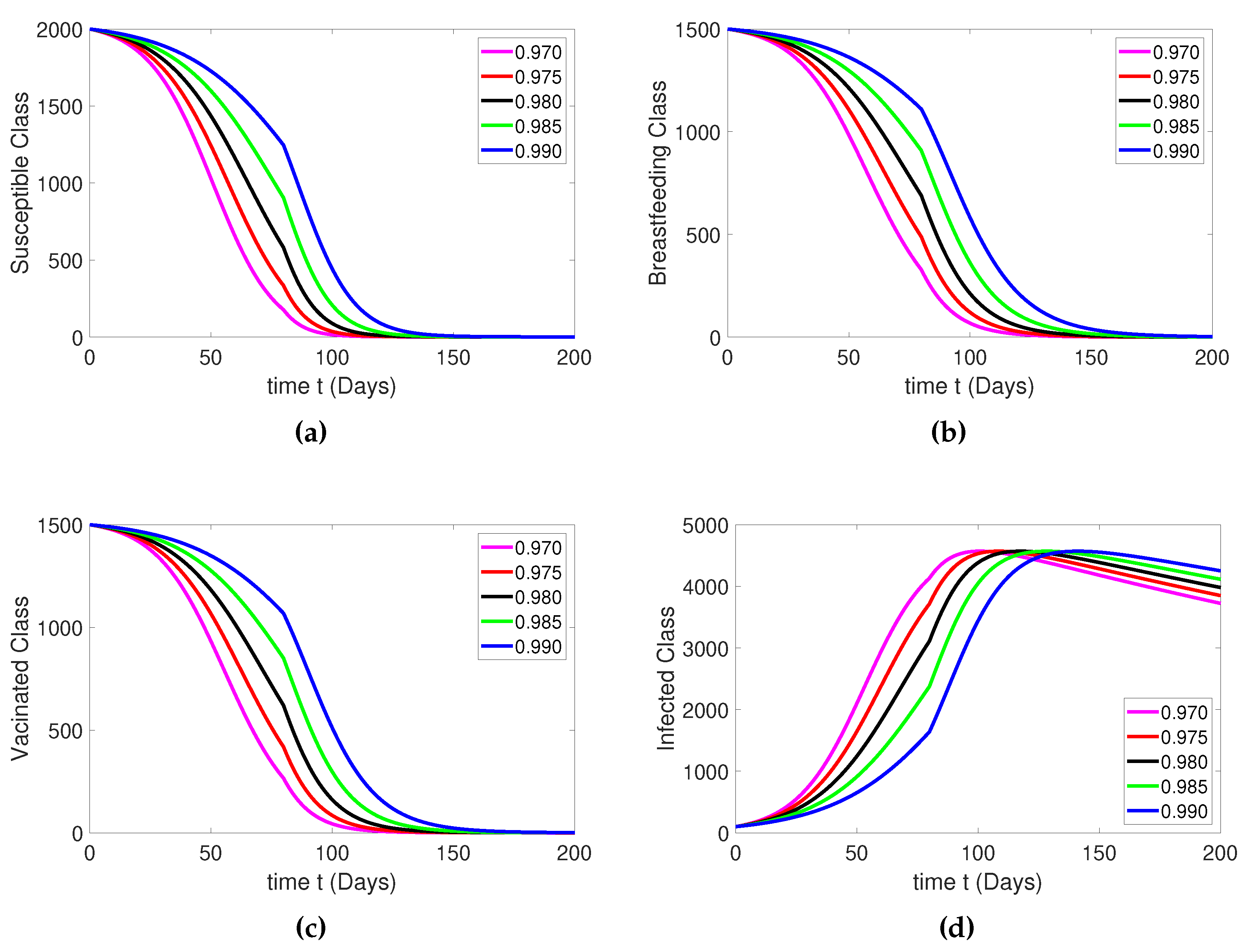
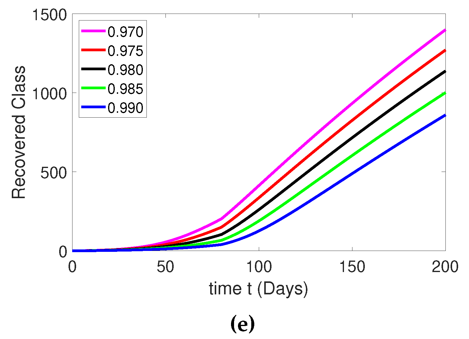
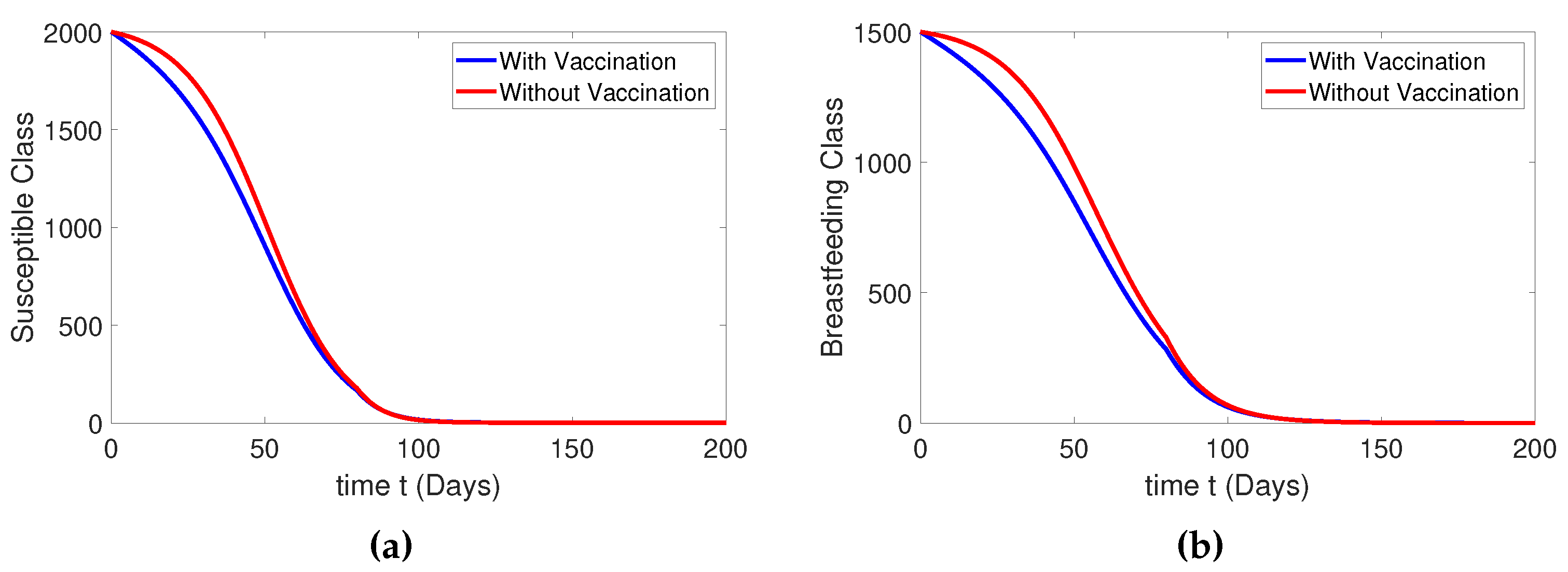
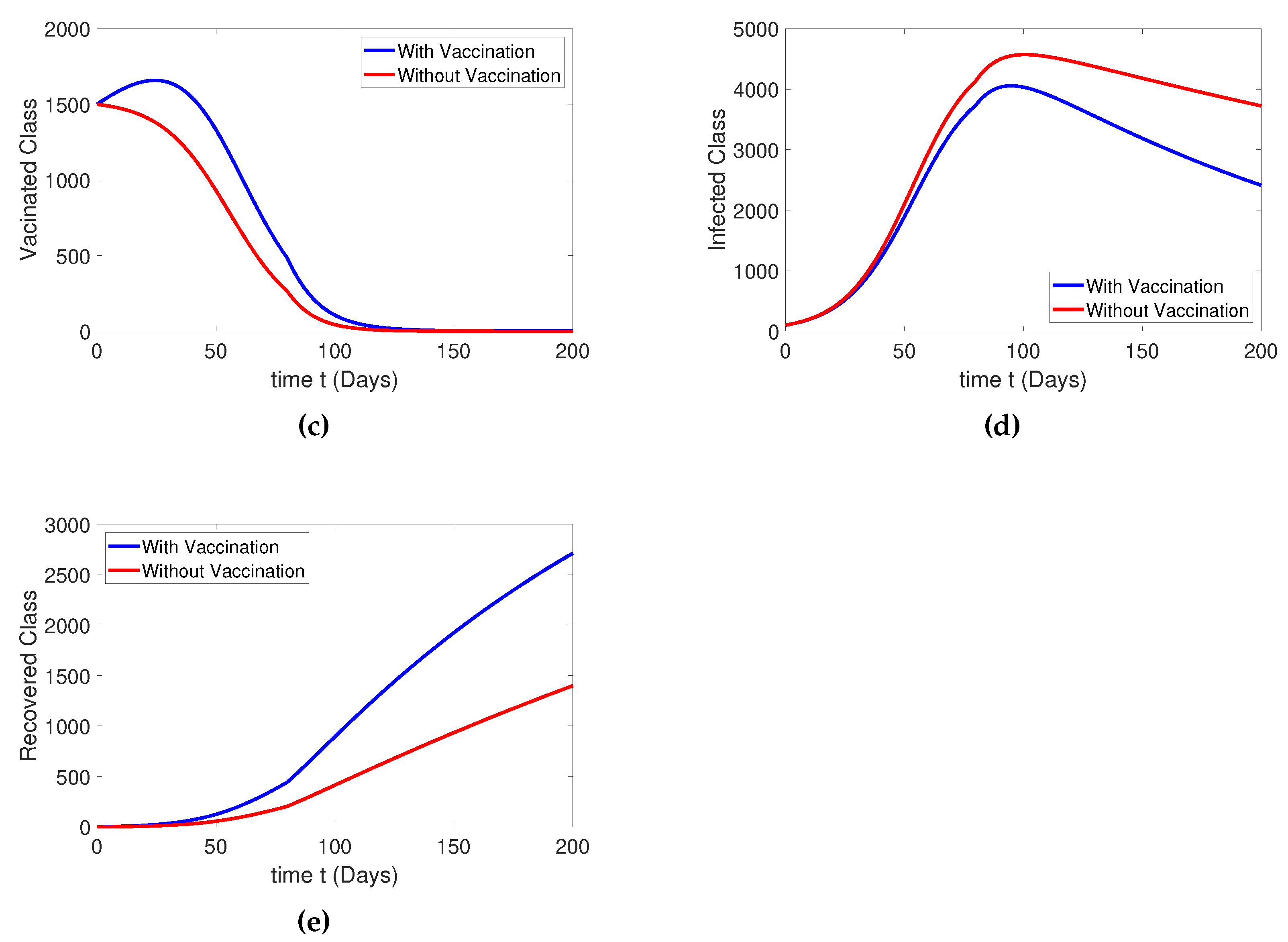
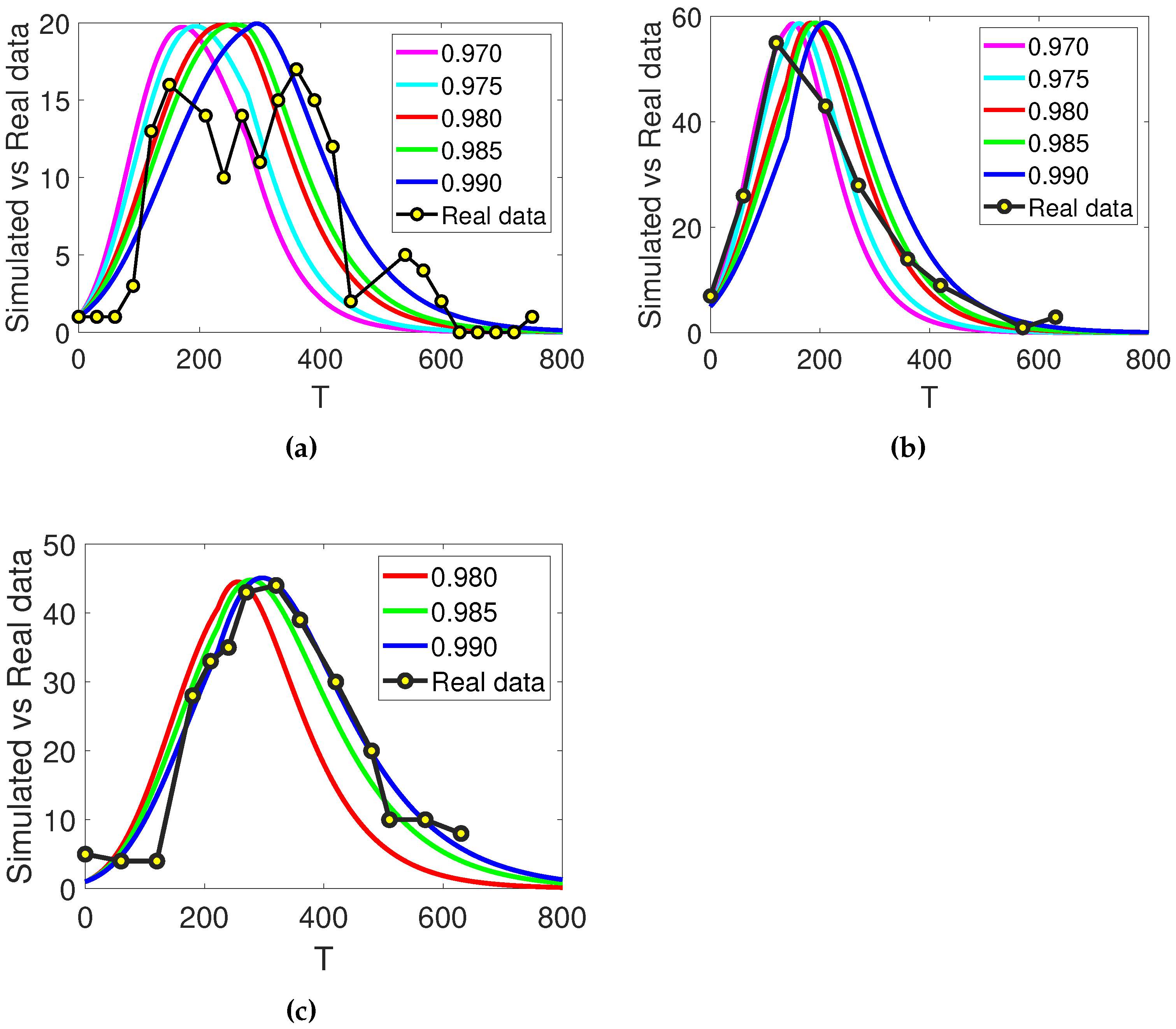
6. Numerical Simulations

Here, we present the graphical simulations of the suggested model (2). The initial conditions are used as [ S 0 , M 0 , V 0 , I 0 , R 0 ] = [ 2000 , 1500 , 1500 , 100 , 0 ] . The simulations for the values of Table 2 are presented in Figure 1a–e. We split the interval into two sub-intervals, which are ( 0 , t 1 ] = ( 0 , 85 ] and ( t 1 , T ] = ( 85 , 200 ] . In the first half-interval, we take the Caputo derivative, and the fractional order ABC operator is used in the second half-interval. Thus, the first half-interval shows the evolution of the considered model (2) in the Caputo operator’s sense, and the curves in second half-interval demonstrate the behavior of the suggested model with various values of m in the ABC sense. In Figure 1a–e, the values of fractional order m are used as ( b l u e , 0.990 ) , ( g r e e n , 0.985 ) , ( b l a c k , 0.980 ) , ( r e d , 0.975 ) and ( m a g e n t a , 0.970 ) .
Figure 1a, depicts the behavior of susceptible individuals. Figure 1b,c demonstrates the evolution of breastfeeding and vaccinated populous. Further, Figure 1d,e demonstrates the effects of the piecewise operator on the evolution of the infected and recovered populous. In Figure 1a, the number of susceptible individuals declines with the passage of time and vanishes after t = 105 . This shows that at small fractional orders, the individuals decreases fast. The breastfeeding population also decreases with time, which becomes stable after t = 130 , as shown in Figure 1b. Furthermore, the vaccinated populous decays with time starting from 1500 individuals. Moreover, the number of infected children increases and reaches its highest point at t = 80 , after which the number of infections gradually decreases. The recovered populous increases with time demonstrate a rapid increase at the lower values of m as compared to the higher values.
For Figure 2a–e, the parameter values are taken into consideration as shown in Table 2 with fractional order 0.98 . Figure 2a,b show the dynamics of susceptible and breastfeeding population with and without vaccination. Similarly, Figure 2c,d demonstrate the behavior of vaccinated and infected individuals. Furthermore, Figure 2e shows the dynamics of the recovered population. From the simulation of the results with and without vaccination, one thing is clear: that vaccination increases the number of recovered individuals and reduces the size of the infected population.
Figure 3a shows a comparison of the simulated data and the real data of the infected children for three years, September 2012 to October 2014 of the Thailand. We have simulated the infected class with real data. The data considered here is interpolated into days. For the simulation, we have considered initial value I 0 = 2 and the parameters m = 0.52 and λ = 0.2 , while the other parameters are used as presented in Table 2. Here, the fractional order m are used as ( b l u e , 0.990 ) , ( g r e e n , 0.985 ) , ( r e d , 0.980 ) , ( c y a n , 0.975 ) , and ( m a g e n t a , 0.970 ) . For the crossover behavior, the interval is split into two intervals, which are ( 0 , t 1 ] = ( 0 , 280 ] and ( t 1 , T ] = ( 280 , 800 ] . The comparison shows that the proposed rotavirus system shows the best-fitted dynamics with the real cases. The piecewise operator positively affects the model dynamics, which makes the simulated data more fitted with the real data, as can be observed for fractional orders 0.990 , 0.980 , , and 0.970 . Figure 3b,c show the comparison between the simulated results and real data for West Africa and the United States of America. For the simulation of Figure 3b, the parameter δ is considered as δ = 0.009 , while the other parameters are considered as presented in Table 2. Similarly, for the simulation of Figure 3c, the parameters are estimated as δ = 0.00108 , ψ = 0.5 , and other parameters are used from Table 2. We observed that the piecewise operators provide a suitable and efficient way to analyze biological models showing the best-fitted dynamics, as observed from the proposed comparison.

7. Conclusions

The concept of piecewise operators is rarely used in the analysis of mathematical models of biomathematics. So, here in this paper, we have provided another application of the piecewise fractional operator in mathematical biology. We have used the fractional piecewise operator to analyze the rotavirus model regarding the effects of vaccination. The important theoretical and numerical properties have been presented for the proposed model. Using the concept of fixed-point results, we have derived results that deals with the existence and uniqueness of the solution. The solution of a nonlinear model is difficult to compute by using an analytical approach. So, we have used the Adams–Bashforth technique to compute the numerical solution of the piecewise fractional model of rotavirus. The stability of the solution has been studied via the concept of Ulam–Hyres stability. We have used MATLAB-18 to depict the numerical results for few fractional orders. We have observed that the simulated data coincide with the real data for different fractional orders.

Author Contributions

Conceptualization, S.N. and S.A.; methodology, S.S.; software, S.S.; validation, M.D.l.S., A.A. and S.N.; formal analysis, S.A.; investigation, S.A.; resources, A.A.; data curation, S.N.; writing—original draft preparation, S.N., S.A. and S.S.; writing—review and editing, S.A.; visualization, M.D.l.S.; supervision, A.A.; project administration, A.A.; funding acquisition, M.D.l.S. All authors have read and agreed to the published version of the manuscript.

Funding

The APC is supported by the Basque Government, Grant IT1555-22.

Data Availability Statement

Not applicable.

Acknowledgments

The authors are grateful to the Basque Government for its support through Grant IT1555-22 and to MCIN/AEI 269.10.13039/501100011033 for Grant PID2021-1235430B-C21/C22.

Conflicts of Interest

The authors declare no conflict of interest.

References

  1. Prathumwan, D.; Trachoo, K.; Chaiya, I. Mathematical Modeling for Prediction Dynamics of the Coronavirus Disease 2019 (COVID-19) Pandemic, Quarantine Control Measures. Symmetry 2020, 12, 1404. [Google Scholar] [CrossRef]
  2. Chamnan, A.; Pongsumpun, P.; Tang, I.M.; Wongvanich, N. Local and Global Stability Analysis of Dengue Disease with Vaccination and Optimal Control. Symmetry 2021, 13, 1917. [Google Scholar] [CrossRef]
  3. Centers for Disease Control and Prevention 2015 Rotavirus: Epidemiology and prevention of vaccine preventable diseases. In The Pink Book: Course Textbook, 13th ed.; Second; CDC: Atlanta, GA, USA, 2015.
  4. Kraay, A.N.M.; Brouwer, A.F.; Nan, L.; Collender, P.A.; Remais, J.V.; Eisenberg, J.N.S. Modeling environmentally mediated rotavirustransmission: The role of temperature and hydrologic factors. Proc. Natl. Acad. Sci. USA 2018, 115, 2782–2790. [Google Scholar] [CrossRef] [Green Version]
  5. Parashar, U.D.; Gibson, C.J.; Bresee, J.S.; Glass, R.I. Rotavirus and severe childhood diarrhea. Emerg. Infect. Dis. 2006, 12, 304–306. [Google Scholar] [CrossRef] [Green Version]
  6. Glass, R.I.; Parashar, U.; Patel, M.; Tate, J.; Jiang, B.; Gentsch, J. The control of rotavirus gastroenteritis in the United States. Trans. Am. Clin. Climatol. Assoc. 2012, 123, 36–52. [Google Scholar] [PubMed]
  7. Glass, R.I.; Parashar, U.; Patel, M.; Gentsch, J.; Jiang, B. Rotavirus vaccines: Successes and challenges. J. Infect. 2014, 68, S9–S18. [Google Scholar] [CrossRef] [PubMed]
  8. Anderson, E.J.; Weber, S.G. Rotavirus infection in adults. Lancet Infect. Dis. 2004, 4, 91–99. [Google Scholar] [CrossRef]
  9. Ruuska, T.; Vesikari, T. Rotavirus disease in Finnish children: Use of numerical scores for clinical severity of diarrhoeal episodes. Scand. J. Infect. Dis. 1990, 22, 259–267. [Google Scholar] [CrossRef]
  10. McNeal, M.M.; Bernstein, D.I. Rotaviruses. In Viral Infections of Humans; Springer: Berlin, Germany, 2014; pp. 713–714. [Google Scholar]
  11. Dennehy, P.H. Transmission of rotavirus and other enteric pathogens in the home. Pediatr. Infect. Dis. J. 2000, 19, S103–S105. [Google Scholar] [CrossRef]
  12. Nitiema, L.W.; Nordgren, J.; Ouermi, D.; Dianou, D.; Traore, A.S.; Svensson, L.; Simpore, J. Burden of rotavirus and other enteropathogens among children with diarrhea in Burkina Faso. Int. J. Infect. Dis. 2011, 15, 646–652. [Google Scholar] [CrossRef]
  13. Wang, Y.; Jin, Z.; Yang, Z.; Zhang, Z.K.; Zhou, T.; Sun, G.Q. Global analysis of an SIS model with an infective vector on complex networks. Nonlinear Anal. Real World Appl. 2012, 13, 543–557. [Google Scholar] [CrossRef]
  14. Wang, Y.; Jin, Z. Global analysis of multiple routes of disease transmission on heterogeneous networks. Phys. A Stat. Mech. Appl. 2013, 392, 3869–3880. [Google Scholar] [CrossRef]
  15. Hochwald, C.; Kivela, L. Rotavirus vaccine, live, oral, tetravalent (RotaShield). Pediatr. Nurs. 1998, 25, 203–204. [Google Scholar]
  16. Jain, P.; Jain, A. Waterborne viral gastroenteritis: An introduction to common agents. In Water and Health; Springer: Berlin, Germany, 2014; pp. 53–74. [Google Scholar]
  17. WHO. Introduction of Rotavirus Vaccines into National Immunization Programs; WHO: Geneva, Switzerland, 2009; Volume 5, pp. 200–209.
  18. WHO. World Health Organisation Statistics Report on Water and Sanitation Program (WSP) in Uganda; Epidemiological March Record 2012; WHO: Geneva, Switzerland, 2012; Volume 88, pp. 224–240.
  19. WHO. Bulletin of the World Health Organisation, Rotavirus and Other Viral Diarrhoes; WHO Scientific Working Group; WHO: Geneva, Switzerland, 1980; Volume 58, pp. 183–198.
  20. Heymann, D. (Ed.) Gastroenteritis, acute viral. In Control of Communicable Disease Manual, 18th ed.; America Public Health Association: Washington, DC, USA, 2004; pp. 224–227. [Google Scholar]
  21. Vesikari, T.; Karvonen, A.; Prymula, R.; Schuster, V.; Tejedor, J.C.; Cohen, R. Efficacy of human rotavirus vaccine against rotavirus gastroenteritis during the first 2 years of life in European Infants: Randomized double-blind controlled study. Lancet 2007, 370, 1757–1763. [Google Scholar] [CrossRef] [PubMed]
  22. Zaman, K.; Dang, D.A.; Victor, J.C. Efficay of pentavalent rotavirus vaccines against severe rotavirus gastroenteritis in infants in developing countries in Sub-Sahara Africa: A randomised, double-blind, placebocontrolled trail. Lancet 2010, 376, 615–623. [Google Scholar] [CrossRef]
  23. Shim, E.; Feng, Z.; Martcheva, M.; Castillo-Chavez, C. An age-structured epidemic model of rotavirus with vaccination. J. Math. Biol. 2006, 53, 719–746. [Google Scholar] [CrossRef]
  24. Cortese, M.M.; Parashar, U.D. Prevention of Rotavirus Gastroenteritis Among Infants and Children: Recommendations of The Advisory Committee On Immunization Practices (ACIP). MMWR Morb. Mortal. Wkly. Rep. 2009, 58, 1–25. [Google Scholar]
  25. Snelling, T.; Markey, P.; Carapetis, J.; Andrews, R. Rotavirus Infection in Northern Territory Before and after Vaccination. Microbiology 2012, 2, 61–63. [Google Scholar] [CrossRef]
  26. Shuaib, S.E.; Riyapan, P. A mathemathical model to study the effects of breastfeeding and vaccination on rotavirus epidemics. J. Math. Fund. Sci. 2020, 52, 43–65. [Google Scholar] [CrossRef]
  27. Sweilam, N.H.; Assiri, T.A.; Hasan, M.M.A. Numerical solutions of nonlinear fractional Schrödinger equations using nonstandard discretizations. Numer. Methods Partial Differ. Equ. 2017, 33, 1399–1419. [Google Scholar] [CrossRef]
  28. Rahman, M.; Ahmad, S.; Arfan, M.; Akgül, A.; Jarad, F. Fractional Order Mathematical Model of Serial Killing with Different Choices of Control Strategy. Fractal Fract. 2022, 6, 162. [Google Scholar] [CrossRef]
  29. Sinan, M.; Ali, A.; Shah, K.; Assiri, T.A.; Nofal, T.A. Stability analysis and optimal control of COVID-19 pandemic SEIQR fractional mathematical model with harmonic mean type incidence rate and treatment. Results Phys. 2021, 22, 103873. [Google Scholar] [CrossRef] [PubMed]
  30. Sweilam, N.H.; Al-Mekhlafi, S.M.; Assiri, T.A. Numerical Study for Time Delay Multistrain Tuberculosis Model of Fractional Order. Complexity 2017, 2017, 1047384. [Google Scholar] [CrossRef] [Green Version]
  31. Ahmad, S.; Ullah, A.; Arfan, M.; Shah, K. On analysis of the fractional mathematical model of rotavirus epidemic with the effects of breastfeeding and vaccination under Atangana–Baleanu (AB) derivative. Chaos Soliton. Fract. 2020, 140, 110233. [Google Scholar] [CrossRef]
  32. Omar, O.A.M.; Elbarkouky, R.A.; Ahmed, H.M. Fractional stochastic modeling of COVID-19 under wide spread of vaccinations: Egyptian case study. Alex. Eng. J. 2022, 61, 8595–8609. [Google Scholar] [CrossRef]
  33. Omar, O.A.M.; Alnafisah, Y.; Elbarkouk, R.A.; Ahmed, H.M. COVID-19 deterministic and stochastic modeling with optimized daily vaccinations in Saudi Arabia. Results Phys. 2021, 28, 104629. [Google Scholar] [CrossRef]
  34. Atangana, A.; Araz, S.I. New concept in calculus:Piecewise differential and integral operators. Chaos Soliton. Fract. 2021, 145, 110638. [Google Scholar]
  35. Abdelmohsen, S.A.M.; Yassen, M.F.; Ahmad, S.; Abdelbacki, A.M.M.; Khan, J. Theoretical and numerical study of the rumours spreading model in the framework of piecewise derivative. Eur. Phys. J. Plus 2022, 137, 1–12. [Google Scholar]
  36. Ahmad, S.; Yassen, M.F.; Alam, M.M.; Alkhati, S.; Jarad, F.; Riaz, M.B. A numerical study of dengue internal transmission model with fractional piecewise derivative. Results Phys. 2022, 39, 105798. [Google Scholar] [CrossRef]
  37. Xu, C.; Alhejaili, W.; Saifullah, S.; Khan, A.; Khan, J.; El-Shorbagy, M.A. Analysis of Huanglongbing disease model with a novel fractional piecewise approach. Chaos Soliton. Fract. 2022, 161, 112316. [Google Scholar] [CrossRef]
Figure 1. The dynamics of the considered model (2) for t 1 = 80 .
Symmetry 14 02641 g001aSymmetry 14 02641 g001b
Figure 2. The dynamics of the model (2) with and without vaccination.
Symmetry 14 02641 g002aSymmetry 14 02641 g002b
Figure 3. The comparison of the simulated and real data with a variety of fractional orders of the model (2) with t 1 = 280 .
Symmetry 14 02641 g003
Table 1. Parameters and their description in model (1).
ParameterDescriptionUnits
( 1 ξ ζ ) Λ Rate of inclusion into class S people/day
Λ ξ Rate of inclusion into class M people/day
Λ ζ Rate of inclusion into class V people/day
φ Rate of breastfeeding of class S 1/day
Υ Rate of vaccination of class S 1/day
ψ Rate of vaccination of class M 1/day
δ Contact rate1/day
ω Rate of waning of antibodies (maternal) from breast milk1/day
ν Rate of waning of vaccine1/day
ς Infection risk reduction due to antibodies (maternal)1/day
λ Infection risk reduction due to vaccines1/day
τ Mortality rate of disease1/day
κ Natural death rate1/day
m Flow rate into the removed class1/day
Table 2. Parameters and their values in model (1).
ParameterBreastfeeding OnlyBreastfeeding and Vaccination
Λ 6.83946.8394
φ 4.9315 × 10 4 4.9315 × 10 4
Υ 00.2
ψ 00.2
δ 0.010.01
ω 5.4945 × 10 3 5.4945 × 10 3
ν 1.3699 × 10 3 1.3699 × 10 3
ς 0.620.62
λ 0.620.62
τ 4.4660 × 10 5 4.4660 × 10 5
κ 3.6529 × 10 5 3.6529 × 10 5
m 8.3333 × 10 2 8.3333 × 10 2
Publisher’s Note: MDPI stays neutral with regard to jurisdictional claims in published maps and institutional affiliations.

