
The 35-Day Cycle of Hercules X-1 in Multiple Energy Bands from MAXI and Swift/BAT Monitoring


Department of Physics and Astronomy, University of Calgary, Calgary, AB T2N 1N4, Canada
*
Author to whom correspondence should be addressed.
Universe 2021, 7(6), 160; https://doi.org/10.3390/universe7060160
Submission received: 23 April 2021
/
Revised: 18 May 2021
/
Accepted: 20 May 2021
/
Published: 23 May 2021
(This article belongs to the Special Issue Universe: Feature Papers − Compact Objects)
Abstract
:Hercules X-1 (Her X-1) has been monitored by MAXI and by Swift/BAT for over a decade. Those observations are analyzed to measure the shape and energy dependence of the long-term average of the 35-day cycle of Her X-1. The cross-correlation (CC) method is used to determine peak times and cycle lengths. Swift/BAT data produces better 35-day times because of the gaps in the MAXI data. Using Swift/BAT-derived times, average 35-day cycle light-curves are created for multiple energy bands: MAXI’s 2–20 keV, 2–4 keV, 4–10 keV and 10–20 keV bands and Swift/BAT’s 15–50 keV band. The durations of the different states of the 35-day cycle are measured better than previously. We find clear changes in X-ray softness ratio with 35-day phase, and detect persistent features in the 35-day cycle. These include column density changes during turn-on of Main High and of Short High states, and persistent absorption dips during the bright part of Main High and of Short High states.
1. Introduction
Hercules X-1 (Her X-1) is a X-ray pulsar with an accretion disk. Her X-1 and its optical companion HZ Her forms an X-ray binary system of active research interest. First discovered in 1971 by the Uhuru satellite, the system has been observed by many missions which have accumulated extensive amounts of data.
Different components in the Her X-1/HZ Her binary system contribute to various phenomena seen in the light-curve on different timescales. Her X-1 has a pulsation period of 1.24 s, and the orbital period of the binary system is 1.7 days. In addition, the X-ray emission of Her X-1 displays a repetitive feature of 35 days in length.
The 35-day cycle was discovered, and shown to have significant variations in length, by [1]. The pulse shape shows a regular progression of changes with 35-day phase [2], and 35-day flux phase and 35-day pulse-precession-phase have been shown to be tied to the same irregular 35-day cycle clock [3]. The cycle is caused by a counter-precessing twisted-tilted accretion disk of Her X-1 [2,4,5]. The cycle sometimes disappears in X-rays, which is called an anomalous low state (ALS) [6]. During those times, the optical cycle is still seen [7], giving evidence that the shape of the accretion disk changes during ALS periods [8,9].
Her X-1/HZ Her can be studied from multiple aspects in detail thanks to the multi-band emissions from the system in X-ray, extreme ultraviolet (EUV), ultraviolet (UV) and optical. Spectral studies of X-ray emissions from Her X-1 include those using GINGA [10], ASCA [11], BeppoSAX [12,13], and AstroSat [14], confirming a blackbody component of ∼0.1 keV. Analyses of UV spectra are given by [15,16] and EUV spectra by [17]. The broadband emission in optical is studied by, e.g., [18,19,20,21].
Long term monitoring observations of Her X-1 by Rossi X-ray Timing Explorer (RXTE) All-Sky Monitor (ASM) were analyzed by [22,23,24] and most recently by [25]. RXTE/ASM operated from 1996 until 2013.
Since 2008, monitoring of Her X-1 has been carried out by MAXI, the Monitor of All-sky X-ray Image on the International Space Station (ISS) [26]. The other main instrument monitoring Her X-1 is the Swift Burst Alert Telescope (BAT) as part of its all-sky monitoring observations [27].
RXTE/ASM and Swift/BAT observations of Her X-1 were analyzed by [25]. In the current work, we analyze the 35-day cycle of Her X-1 using MAXI and Swift/BAT data to produce multiband light-curves of the 35-day cycle. The data sets and our cross-correlation (CC) analysis method are described in Section 2. In Section 3, we obtain the 35-day cycle shape in the different energy ranges covered by MAXI and BAT. The timing of the 35-day cycle in different energy bands is compared. Softness-ratios vs. 35-day phase are used to examine the spectral changes over 35-day cycle. In Section 4, we further analyze and discuss the main results, and summarize in Section 5.
2. Data and Analysis
2.1. Data
Here we analyse public observations of Hercules X-1 from MAXI and Swift/BAT instruments. MAXI monitors Her X-1 in the energy band 2–20 keV (hereafter “Total”), and in three narrower bands available simultaneously: 2–4 keV, 4–10 keV, and 10–20 keV (hereafter Band 1, 2 and 3, respectively) [26]. The Swift/BAT instrument monitors sources in the 15–50 keV band and is described in [27].
For MAXI, data products (version 7L) were downloaded from the website provided by RIKEN, JAXA and the MAXI team.1 The data contained a total number of 31,927 observation intervals, with flux in unit of cts sec cm from August 2009 to June 2020. MAXI observations are labelled with MJD in ISS time. For Swift/BAT, we downloaded the data for the energy range of 15–50 keV, covering 14 years of observation with 71,165 points from February 2005 to November 2019. Swift/BAT observations are labelled with MJD in TT time. For both data sets, the correction from ISS or TT time to Barycentric Dynamical Time (TDB) is small (∼ s) and is ignored compared to the time resolution of our analysis, which is ∼0.01–0.02 of a 35-day cycle (∼860–1720 s). Similarly, the maximum correction for Her X-1 to solar system barycentre is ∼268 s, small compared to our time resolution, is ignored for this analysis.
Figure 1 shows two examples of MAXI and Swift/BAT data on Her X-1 over a 35-day cycle. This illustrates that both MAXI and BAT can clearly detect the 35-day cycle of Her X-1. The observation times are generally not simultaneous and both instruments have significant noise level. e.g., near MJD 56,228 and 56,229.7, MAXI detects two binary eclipses which are not seen in BAT, and around MJD 56,221 there is a gap in the MAXI data which is well covered by BAT data.
2.2. Analysis
In order to determine the occurence times of 35-day cycles we use the cross-correlation (CC) method [22,25]). The CC method includes template fitting, and in our iterative application of the method, it has the advantage that the template is derived from the data. The CC method is used because it has better properties compared to previously used methods, such as defining a fiducial point on the light-curve, like Turn-On (TO) [23]. Defining a fiducial point is difficult when the light-curve has strong variability, like the 35-day cycle of Her X-1: different fiducial points give different results because of the changing shape of the light-curve. For TO, there is the further difficulty that the TO occurs over a period of many hours: e.g. the TO observed by [28] took place over a period of 2.0 d (0.057 of a 35-day cycle) inhibiting an accurate timing of the 35-day cycle.
For most observations, because of limited observation time and earth occultation gaps, only a partial or fragmented light-curve can be obtained. The CC method is better in that it uses all available observations over a 35-day cycle and gives the time when the average 35-day cycle light-curve matches the observations. Our method of CC analysis is applied iteratively [22], which means it also produces a reliable average light-curve based on the observations.
The iteration process is as follows: an initial template light-curve is cross-correlated with the data to measure 35-day cycle peak times; the peak times are used to measure individual cycle lengths; the peak times and cycle lengths are used to create a new average 35-day light-curve. The new 35-day light-curve then replaces the initial template. This process is repeated until convergence. We took the convergence criterion as the condition that the difference in 35-day cycle peak times between one interation and the previous iteration to be less than 0.1 days. To avoid aliasing with the orbital period (from peaks in the cross-correlation function when eclipses line up), the data near neutron star eclipse, in orbital phases 0–0.16 and 0.84–1.0 were removed prior to CC analysis.
We used the peak of Main High (MH) state to define 35-day phase 0. That provides a better reference point than using TO. This is because TO is defined differently in different papers and because the 35-day cycle shape is quite variable, especially when measured with high sensitivity instruments such as RXTE/PCA (see the light-curves in [22]). For the average 35-day cycle shape measured with Swift/BAT [25], TO occurs at 35 day phase 0.13 earlier than peak of MH.
2.2.1. Initial MAXI Analysis
MAXI observations have long data gaps because of the observing limits from the International Space Station: typical observations of Her X-1 last ∼44 days followed by a data gap of ∼28 days. As a result, our previous cross-correlation (CC) method [25] does not directly work on this data. Thus, we made changes to the method to be able to deal with observations with large data gaps. The modified CC method is described in Appendix A.
We apply the CC method with the initial input template from the Swift/BAT analysis of [25]. After calculating the CC function for all points in the MAXI data, peaks of CC were detected and thus the MJD time of MH peaks. Using the new times of MH peaks (times of 35-day phase 0), the new phases of each data point with index k are recalculated2. The data are binned in new 35-day phase to create a new template. The process is repeated, as described in [25], until the set of 35-day MH peak times and the template converge.
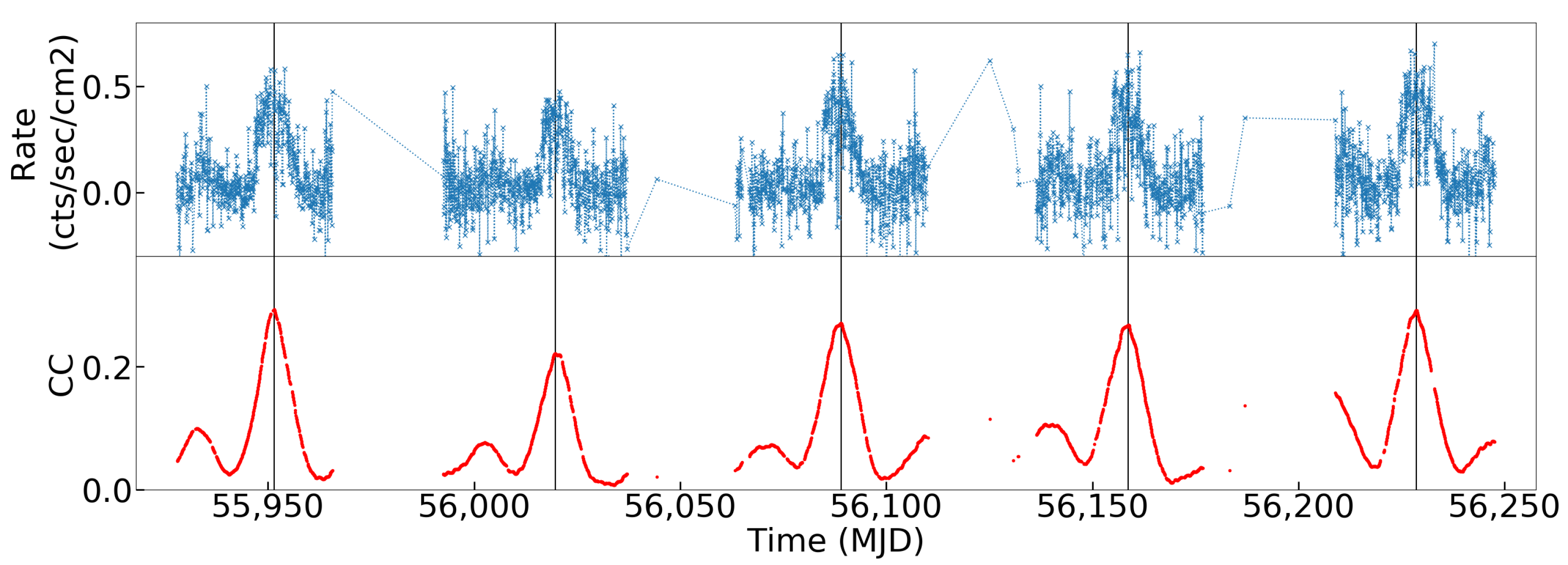
The MH peak times of individual cycles and template shape converged quickly for MAXI, thus three iterations of CC were performed on the MAXI data. The MAXI data and the CC function from the last iteration are shown for a day section of MAXI data in Figure 2. The peaks in CC value find the MH peaks of the 35-day cycles as expected.
The time period of MAXI observations covers a total of 112 35-day cycles, of which 73 peaks are detected in the last (third) run by the modified CC method. Cycle # 59, 109, 111, 138 have weak CC peaks and are identified manually. Because MAXI covers a similar observation time period to Swift/BAT, we assign the cycles with the same cycle number as those from Swift/BAT in Table 1 of [25].
The 77 MH peak times measured from the data are used to calculate the cycle lengths. For the missing cycles, caused by MAXI data gaps, we estimate peak times and cycle lengths by dividing the difference of detected MH peak times by the number of intervening cycles. We name these estimate peak times and cycle lengths as as interpolated peak times and cycle lengths. From the 77 detected MH peak times (including the four weak cycles), the average cycle length of MAXI is 34.32 days (with standard deviation3 SD days). The average from all 112 MH peak times (including 35 interpolated ones) during the MAXI observation time is 34.76 days (SD days). The SD for all cycles is lower because the interpolated cycle lengths are averages over 2 or 3 cycles, thus have smaller fluctuations.
The average 35-day light-curve (i.e., the template) created using the 35-day cycle timings from the CC analysis of MAXI 2–20 keV data is not shown here. However, it is nearly the same as the MAXI average 35-day light-curve created using 35-day cycle timings from the BAT data CC analysis, which is discussed in Section 3.1 below.
2.2.2. Swift/BAT Analysis
We apply the new CC method to the Swift/BAT data, with iterations until convergence for the 35-day cycle times and average 35-day cycle shape. The new CC method is described in Appendix B. The main difference from the CC method used by [25] is that the new procedure uses binning the data rather than interpolating the data to bin centers to calculate the template. The new method allows calculation of errors on the average 35-day light-curve. The resulting Swift/BAT 35-day cycle timings are unchanged from those given by [25], so we refer to that paper for the timings.
2.2.3. Adopted Method for 35-Day Cycle Analysis
A total number of 104 cycles are present during the overlap time period between MAXI and Swift/BAT (Cycle - ), of which 41 cycles are detected by CC method in both missions. For these 41 cycles, we compared the scatter in cycle lengths found by Swift/BAT and by MAXI. The mean and standard deviation for BAT-derived cycle lengths are 34.80 and 1.09 days, compared to 34.03 and 5.71 days for MAXI-derived cycle lengths. BAT measures the cycle lengths with less scatter, which is consistent with using BAT as a better reference for MH peak times.
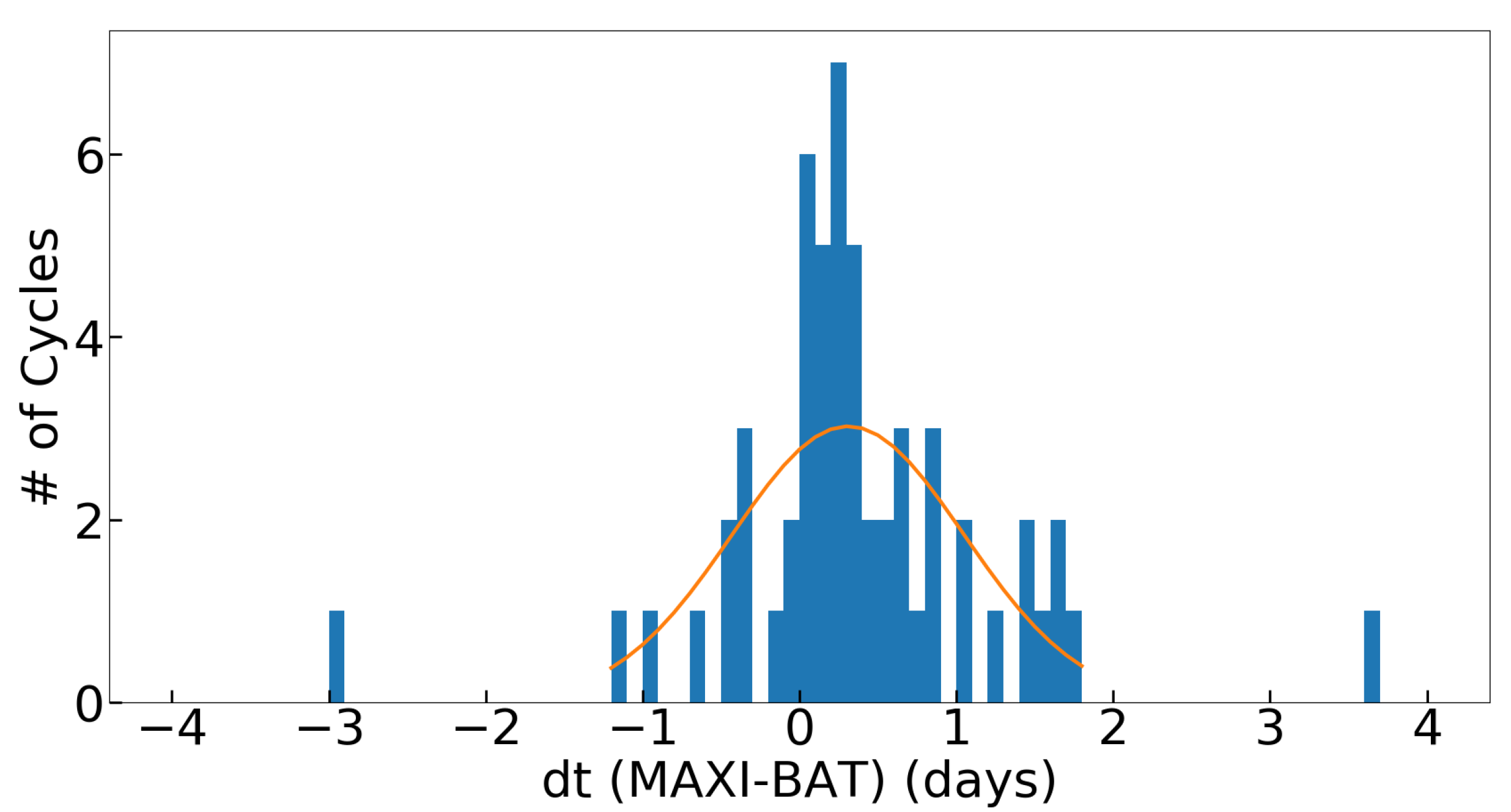
We define the difference between MH peak times of MAXI and BAT as with and the MH peak times determined by CC analysis on MAXI and BAT data, respectively. The histogram of is shown in Figure 4. can be seen in Figure 1 for the data from cycles 80 and 97. (2–20 keV band) is generally later than (15–50 keV band). The mean delay (mean of ) is 0.343 days ( in 35-day phase) with SD of 1.010 days. We fit the histogram of with a Gaussian, shown in Figure 4. The best-fit parameters of the Gaussian are consistent with the mean and SD of . The mean is consistent with the mean delay of RXTE/ASM (2–12 keV) with respect to Swift/BAT of days [25]. This result is not surprising because MAXI has a similar energy band to the 2–12 keV band of RXTE/ASM.
We compared the MH peak times from the CC analysis on MAXI 2–20 keV data with those from Swift/BAT data. We find the Swift/BAT MH peak times are a better and more complete measure of the cycle lengths than those from the MAXI data because of the data gaps in the MAXI data. Thus in our final analysis, we use MH peak times and cycle lengths derived using the Swift/BAT CC analysis as a common reference to calculate 35-day phases of all data for MAXI and Swift/BAT. Those values are listed in Table 1 in [25].4
3. Results
3.1. 35-Day Cycle Average Light-Curves from MAXI and Swift/BAT
The MAXI and BAT average 35-day light-curves are compared in Figure 5. The two different vertical axes are chosen so that the zeros and maxima of the light-curves match. The mean countrates (units ct s cm) are given in Table 1 for the different states of the 35-day cycle. The ratios of mean SH rate to mean MH rate are 0.235 (±0.010) and 0.212 (±0.007) for MAXI and BAT, respectively. Thus relative to MH, SH is brighter (1.9) in the lower energy band of MAXI.
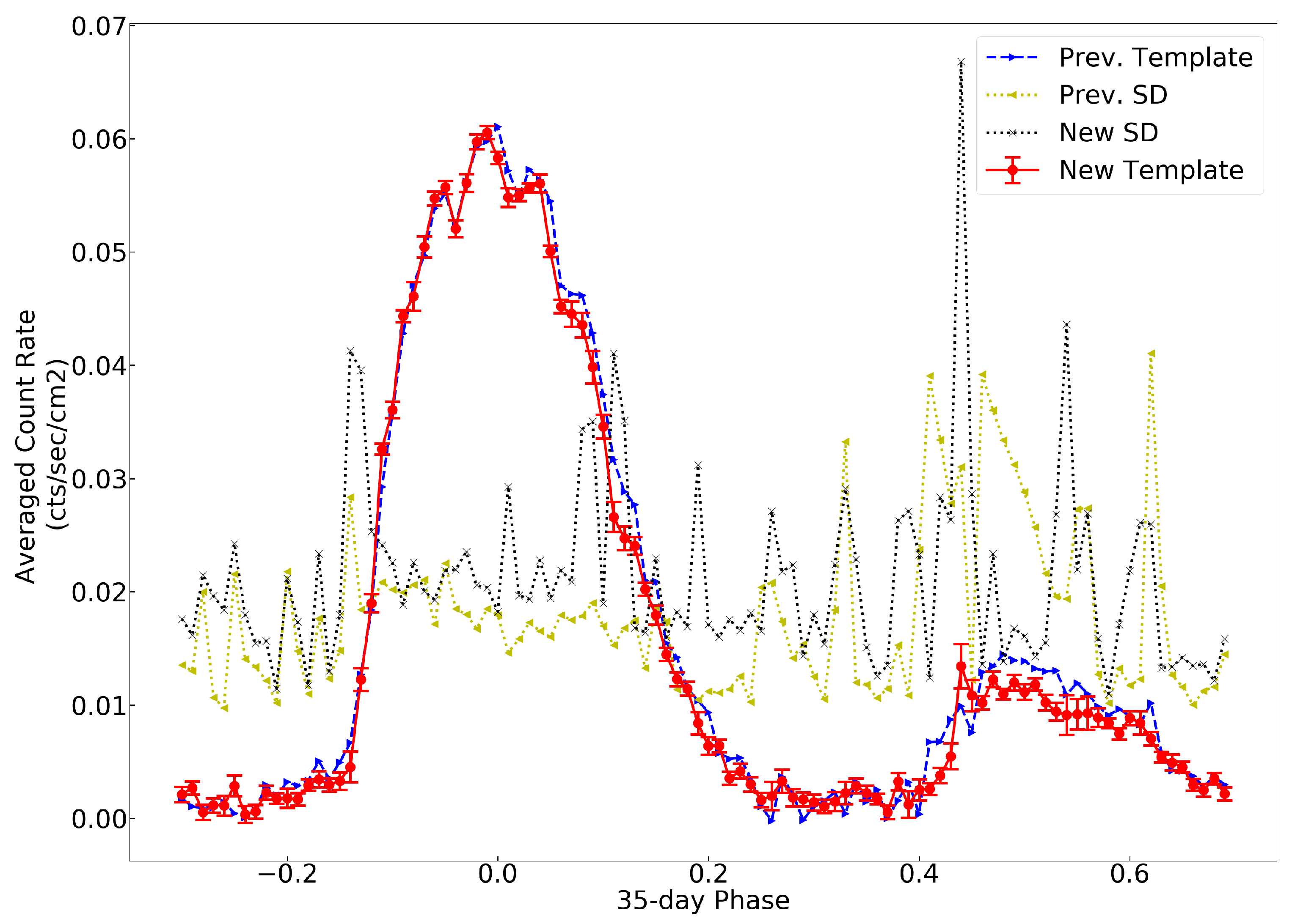
The two light-curves approximately agree in shape, and have similar relative SD-to-rate ratio. MAXI shows higher SD during MH than BAT, but the relative SD agrees between MAXI and BAT during the other states of the 35-day cycle. The BAT relative SD shows larger fluctuations than the MAXI relative SD, likely because the counts in each bin are smaller for BAT, so that Poisson fluctuations in the counts rates are larger.
To better understand the behaviour of SD, we note that SD of each bin measures the mean level of fluctuations of all the data in that bin. The error for each bin (plotted as error bars in Figure 5) measures the measurement error of the mean of all data in that bin (, with the number of data points in bin k and the measurement error of data point i in bin k). The errors are similar for all bins because the numbers of data points (from MAXI or from BAT) are approximately equal for all bins, and statistical errors are similar for all bins. The SD, in the case that the only cause of data fluctuations is measurement noise, is the same as the data measurement error, which is ≃ larger than the error in the mean for bin k. However in the case of intrinsic source variations, the SD is larger than the error.
Here, typical is ∼300 for MAXI and ∼700 for BAT. The individual data measurement errors are ∼0.1 count cm s for MAXI and ∼0.012 count cm s for BAT. These correspond to an error in the mean count rate per bin of ∼0.06 count cm s for MAXI and ∼0.0005 count cm s for BAT, similar to the values calculated in detail for Figure 5. The expected SD, if measurement error dominates, is the data measurement errors, i.e., the expected SD is ∼0.1 count cm s for MAXI and ∼0.01 count cm s for BAT. From Figure 5, it is seen that the MAXI SD is similar to that from measurement errors for SH and low states, but is significantly higher for MH, indicating source variations dominate for MH. For BAT, the same result is found: the SD is signficantly higher than expected from measurement errors for MH, but similar to that expected for SH and low states (LS).
There are large peaks in SD for BAT at TO to MH (35-day phase −0.13) and TO to SH (35-day phase 0.44), and during decline of MH (35-day phase 0.06 to 0.25) and decline of SH (35-day phase 0.52 to 0.71). These peaks in SD are expected in the disk occultation model of the 35-day cycle [29]. This is because the timing of TO and of decline are determined by the crossing of the line-of-sight by the outer disk edge (for TO) and by inner disk edge (for decline), which are sensitive to changes in disk shape. In addition to the large peaks in SD for BAT there are small oscillations in SD for both MAXI and BAT, which number about 20 for each case. Because there are ≃20 orbital periods in a 35-day cycle, this could be an aliasing effect which was not fully removed when we omitted the eclipse data from the data set prior to the CC analysis.
3.2. Spectral Changes Over the 35-Day Cycle
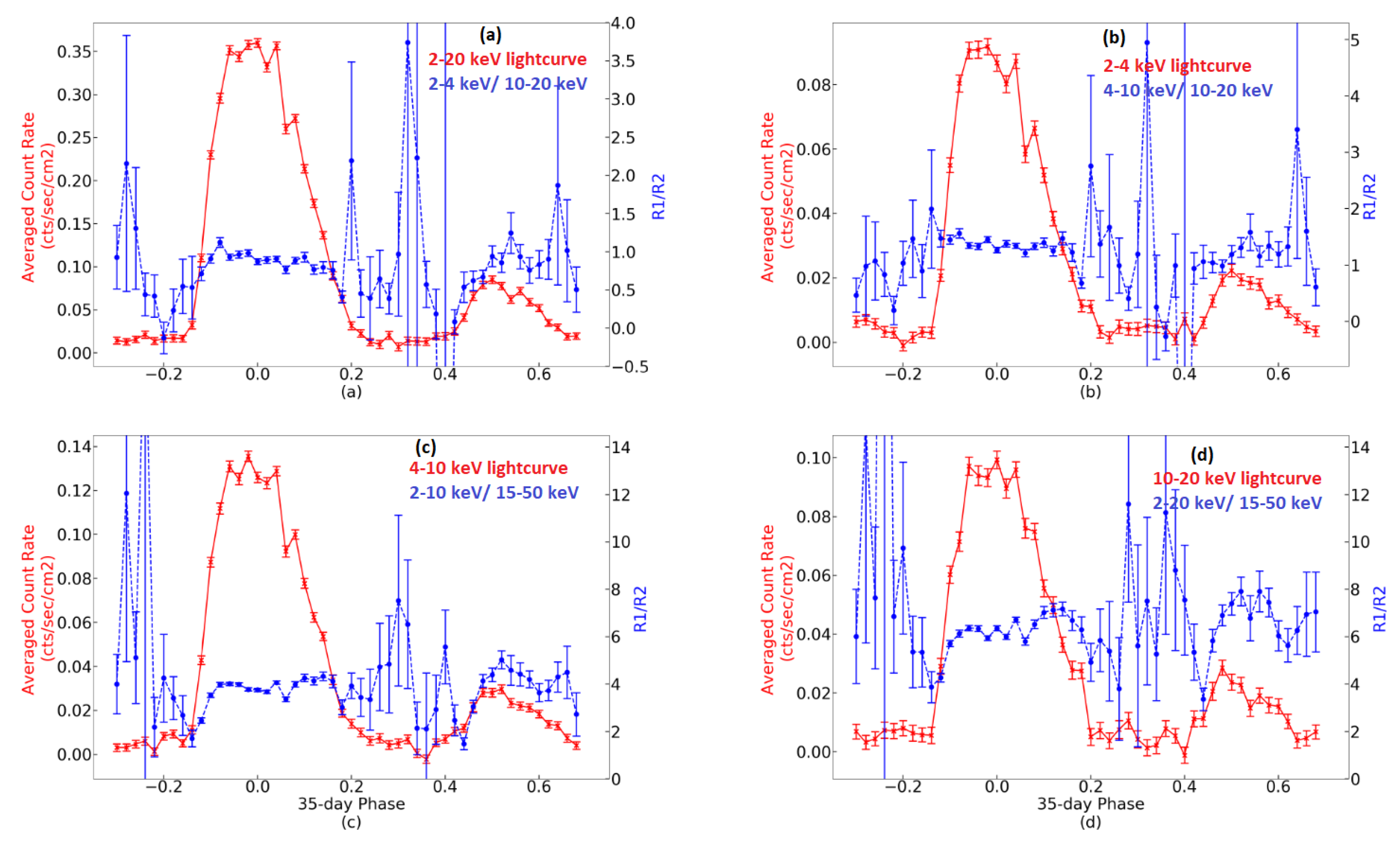
35-day light-curves with 50 bins were created for the energy bands 2–4 keV, 4–10 keV and 10–20 keV of MAXI and for the 15–50 keV band of Swift/BAT. We followed the procedure as given in Appendix B using BAT 35-day cycle times as a reference. Figure 6 shows the light-curves vs. 35-day phase for the MAXI Total (2–20 keV) and the three MAXI energy bands. Also shown are the softness ratios 2–4 keV/10–20 keV, 4–10 keV/10–20 keV, 2–10 keV/15–50 keV and 2–20 keV/15–50 keV.
4. Discussion
4.1. Timing of 35-Day Cycles
Here we discuss the results related to timing (MH peak times and cycle lengths) of the 35-day cycle of Her X-1, derived from the MAXI and Swift/BAT data.
4.1.1. Distribution of Orbital Phases of MH Peak
Orbital phases of MH peak were determined from the CC analysis on MAXI data. We find that the histogram of orbital phases is fit by a large contribution from a uniform distribution plus a smaller contribution from a Gaussian distribution centered on orbital phase 0.5. A similar analysis was done for CC analysis of Swift/BAT data by [25]. Figure 7 shows the histogram of the orbital phases of peak of MH from MAXI CC analysis and from Swift/BAT CC analysis. If the effect was intrinsic to the system, we should have found an orbital phase distribution for MAXI which was delayed from that for Swift/BAT by 0.343 days (0.2 in orbital phase) contradicting what was found.
We believe instead that both results, i.e., the small contribution to a peak centered on orbital phase 0.5 for both BAT and MAXI analyses, are caused by selection effects. The fit times of MH peak tend to avoid the faintest part of the orbital light-curve. In particular, Ref. [30] showed orbital light-curves measured by the RXTE/PCA, averaged for all data (their Figure 4), and separate light-curves for each orbit in MH state and in SH state (their Figure 5). The fainter parts of the orbital light-curve are orbital phases ∼0 to 0.15 and ∼0.65 to 1.0. This selection effect would result in lower efficiency of detection of MH peak times during those orbital phases. This would result in a peak near orbital phase 0.5 on top of a uniform distribution of phases for both MAXI and BAT data. This explanation is more consistent than that the peak at orbital phase 0.5 is intrinsic to Her X-1.
The current results are compared previous work. Previous work referenced the 35-day cycle to TO rather than to peak of MH (see also Section 4.1.3 below). The first evidence that TO occured at specific orbital phases, 0.2 and 0.7, was presented by [1], with 9 observed TOs were concentrated near those orbital phases. The study of the 35-day cycle by [23] assumed TOs occured only at orbital phase 0.2 and 0.7 to create average 35-day light-curves for 0.2 and for 0.7 TOs. TOs measured using the CC method applied to RXTE/ASM data were presented by [22], which showed a uniform distribution of orbital phases. However, Ref. [25] analysed a larger set of RXTE/ASM data and found that the errors in RXTE/ASM TO times were large enough that the the result by [22] should be regarded as inconclusive.
Because of the regular change of pulse-shape with 35-day phase [2], it has been possible to track the cycle lengths and TO times using measurements of pulse shape [3]. A comparison of TOs determined by rise of flux with TOs determined by pulse-shape-phase was shown in Table 1 of [3]. The uncertainties in TO times were typically 0.29 in orbital phase for both flux-determined TOs and pulse-shape-phase determined TOs. TOs from [3] were found to be consistent with 0.25 and 0.75 orbital phases within the ∼0.29 phase error of TOs. The errors in 35-day phase measured using MH peak from the current CC analysis on the Swift/BAT data are ∼0.5 days. There is additional error in converting from MH peak to TO which comes from the variation in 35-day cycle length, which is ∼0.8 day. Thus the error in TO phase from the CC analysis is ∼1 day (0.6 in orbital phase). This precludes a definitive test of distribution of TO orbital phases with the current analysis.
4.1.2. 35-Day Cycle Lengths
The large gaps in the MAXI data compared to Swift/BAT data yield the result that the Swift/BAT 35-day cycle times are the most accurate. Previous analysis of RXTE/ASM and Swift/BAT data [25] found that the BAT 35-day cycle times were most accurate because of the larger noise of the ASM data. The mean cycle length is 34.79 days with standard deviation of 1.1 days The list of Swift/BAT-derived 35-day cycle lengths and peak times is given in [25].
4.1.3. Relation between 35-Day Cycle Peak and Turn-On
The TO to MH for Her X-1 was observed in detail with RXTE/PCA by [28], which noted that there have been very few observations of TO. There have been 3 pointed observations prior 1980, plus those of [2,14,28]. For example, the observation of [28] covered the TO period but ended prior to peak of MH. This is typical because the interval between TO, which lasts anywhere from a few hours [2,14] to ∼40 h [28], occurs on average 4.5 days prior to peak of MH [25].
We defined CC peak, or equivalently MH peak, as 35-day phase 0, whereas previous studies often used TO to define 35-day phase 0. One definition of TO is the time during rise to peak when the flux reaches a fixed percentage (e.g., 20%) of its peak value.5 In the Swift/BAT average 35-day light-curve of Figure 5, TO happens at phase or in 35-day phase, using our reference for 35-day phase 0. TO measured in the 15–50 keV band is on average 4.52 days, or 2.66 binary orbits prior to MH peak.
In the MAXI average 35-day light-curve of Figure 5, TO happens at phase or in 35-day phase. Thus TO in the MAXI 2–20 keV band is later by 0.35 days or ≃ in 35-day phase Compared to the TO for Swift/BAT. This agrees well with the average -day difference between individual MH peak times derived from CC analysis on MAXI data and on Swift/BAT data (Figure 4). The agreement between the two shows that on average the CC-derived peak times from MAXI data are accurate, although the scatter is larger than times derived using Swift/BAT data.
4.2. 35-Day Cycle Long-Term Average Light-Curve
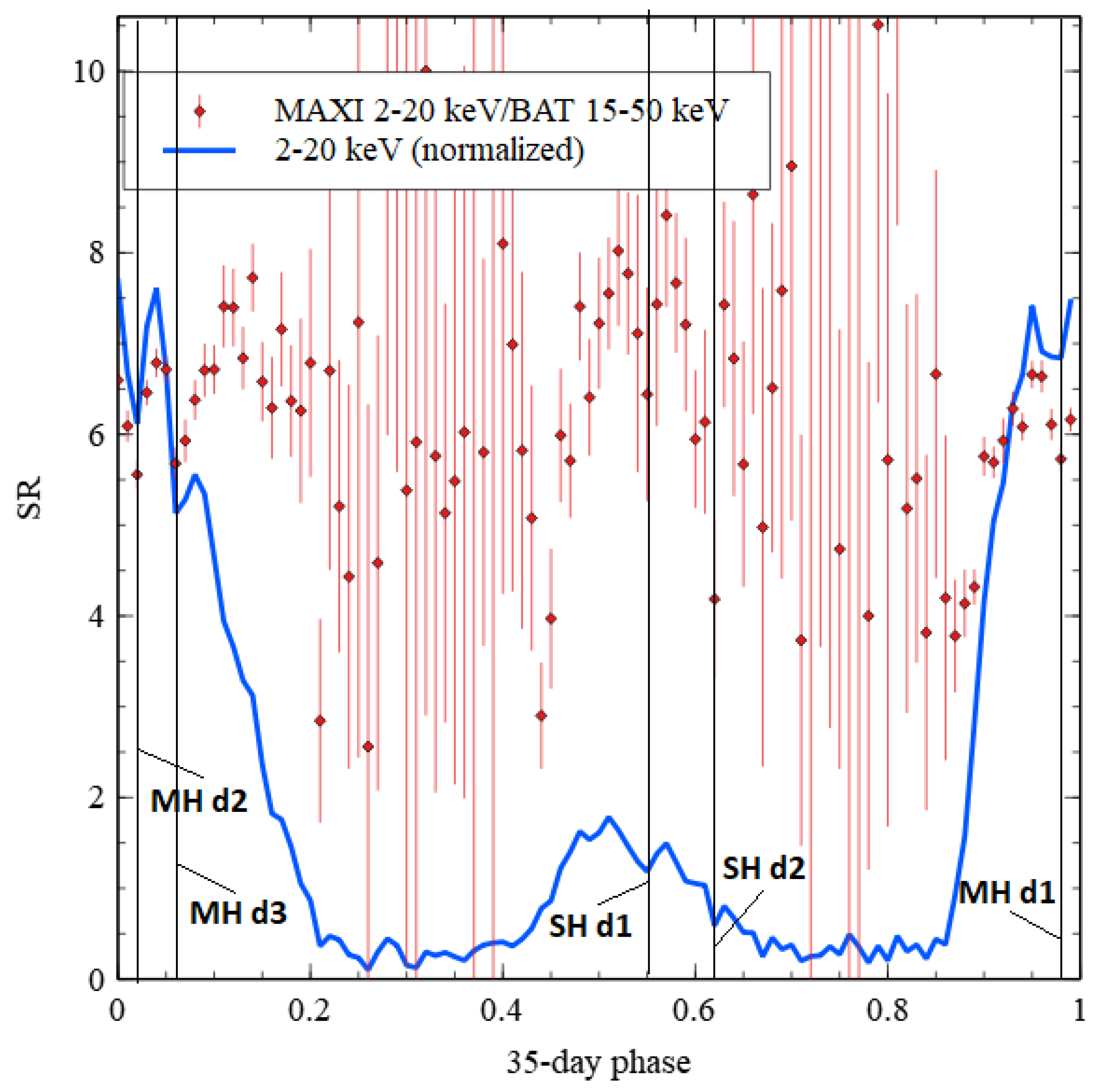
The more-accurate Swift/BAT derived times were used to construct average 35-day light-curves from BAT and MAXI data. These MAXI and BAT light-curves (Figure 5) are the best long-term average 35-day light-curves yet constructed for Hercules X-1, with more accurate 35-day phase alignment than previously possible. Details not previously detectable are now seen in these light-curves. We add basic spectral information by calculating the MAXI 2–20 keV/BAT 15–50 keV SR. This is shown in Figure 8 along with the rescaled (normalized) MAXI light-curve.
4.2.1. Timing of the States of the 35-Day Cycle
The widths and shapes of the different states of Her X-1 are better measured than before. From the light-curves we can identify the well known MH, SH and LS, and the TOs and declines of MH and SH states. The 35-day phases of these features can be given more reliably than before because the long-term average light-curve has now been measured better than previously.
The MH state starts with TO. TO is gradual, best characterized at high sensitivity for a single cycle by [28], with amalgamated RXTE/PCA light-curves given by [30]. Because most previous observations have been carried out in bands similar to the MAXI 2–20 keV band, we use that band to define the states. From Figure 5, it is seen that the 15–50 keV BAT light-curve has essentially the same timing for the different states, with the exception that MH TO, and likely SH TO, start earlier by 0.35 days or 0.01 in 35-day phase.We define MH TO as the period between the first detection of strong absorption at the end of LS until the SR reaches its normal value for peak of MH. Comparing the MAXI 2–20 keV light-curve and 2–20 keV/15–50 keV SR (Figure 8), MH TO starts at 35-day phase 0.86 to 0.87 and ends at 35-day phase 0.94 to 0.95 (the uncertainty in determining the phases is ≃).
MH state lasts from end of TO until beginning of MH decline, which happens at 35-day phase 0.05 to 0.06. MH decline is characterized by decreasing 2–20 keV count rate without corresponding decrease in 2–20 keV/15–50 keV SR. The end of MH decline is characterized by 2–20 keV count rate reaching LS values. This happens at 35-day phase ≃0.25.
The first LS, LS1, lasts from end of MH decline until SH TO. SH TO is characterized, like MH TO, by first detection of strong absorption after LS1. This happens at 35-day phase 0.43 to 0.44. The end of SH TO is characterized by SR reaching its normal value for peak of SH, which happens at 35-day phase 0.48 to 0.49. SH decline sets in nearly immediately ([29]) characterized by declining flux with no change in SR, at 35-day phase 0.51 to 0.52.
SH decline ends when the count rate reaches normal LS values. This happens at 35-day phase ≃0.71. LS2 lasts from end of SH decline until MH TO starts at 35-day phase 0.86 to 0.87. Table 2 summarized these results.
Notable features of the 35-day cycle are as follows. The center phase of MH is 0.00 and center phase of SH is 0.50: these are separated by exactly 0.50 in 35-day phase, to the accuracy that we can measure. This supports the disk occultation model for the 35-day cycle, which predicts a 0.50 phase difference between peak of MH and peak of SH (Figure 3 of [29]). The decline of MH and of SH are both measured to last 0.195 in 35-day phase. In the disk occultation model, the inner edge of the disk blocks the line of sight, and the inner edge is expected to be ionized so that there is no clear absorption signal [2] during decline.
The SH is shorter than MH because the observer’s line-of-sight is blocked by the inner disk edge sooner for SH than for MH ([2,29]). The same effect causes the TO for SH to be shorter than that for MH. The duration of LS1 and LS2 are not expected to be equal because the duration is set by the twist and tilt of the disk combined with the observer’s inclination above the orbital plane (Figure 3 of [29]). For observer inclination of 90, one has LS1 and LS2 of equal duration, MH and SH are the same, and MH and SH TO are the same (but TOs still differ from declines). No other model than the disk occultation model,6 that we are aware of, can match the observations of state durations and SR changes during TOs and declines.7
4.2.2. Delay of Turn-On at Lower Energies
Because the same 35-day phase 0 timings are used for both data sets, we can detect an absolute difference in timing in the peak of the 35-day cycle between BAT (15–50 keV) and MAXI (2–20 keV). From Figure 5 it is seen that the rise to peak in the softer X-ray band is delayed with respect to the hard X-ray band by ≃0.35 days. In contrast to the rise to peak, the decline of MH in both templates is nearly simultaneous. To quantify this, we selected the early part of MH TO from BAT and MAXI light-curves and the intermediate part of decline (after the dips seen in Figure 8 up to 35-day phase 0.2). These were least-squares fit with linear functions to find the x-intercepts. The difference in x-intercepts for the fit to TO for MAXI 2–20 keV compared to that for BAT 15–50 keV was 0.008 in 35-day phase.8 This confirms that the TO in the MAXI 2–20 keV band is delayed compared to the TO in the BAT 15–50 keV band. The difference for decline was 0.0002 in 35-day phase, which is not significant. These results are consistent with those from comparison of the RXTE/ASM 2–12 keV average 35-day light-curve with that of Swift/BAT [25], but are better constrained here.
The delay in rise to peak at lower energies is consistent with absorption by cold matter. TO to MH occurs when the cold matter of the outer disk moves out of the line of sight, thus TO is accompanied by an observed decrease in cold matter absorption with time [28,32]. This is a further confirmation of the disk occultation model for the 35-day cycle (e.g., [2,29]).
4.2.3. New Detection of Persistent Dips
The presence of dips in Her X-1 has been known since their discovery [1]. Observations of dips are reviewed in [33], which also includes a study of all dips observed by RXTE/PCA over a decade of observations which includes dips from 24 MH, 10 SH and 14 LSs over 35 different 35-day cycles. Most previous studies only consider a few dips [34,35]. Dip occurence as a function of orbital phase and 35-day phase was determined by [33], with a predominance of the dips occuring during orbital phases 0.6 to 0.93 (pre-eclipse dips). Figure 3 of [33] shows the 35-day phases of dips. There is no clear set of 35-day phases at which dips occur, except that they do not occur during LS. The occurence of dips vs. 35-day phase is highly biased by the uneven observation times vs. 35-day phase, shown in Figure 3 of [30]. The exposure times are concentrated in MH, 35-day phases ∼0 to 0.25, and SH, phases ∼0.55 to 0.75, with almost no observations in LS.
An important factor for dips is determination of their 35-day phase. As shown by [22], RXTE/ASM data gives TO times, and thus 35-day phase 0, with formal uncertainties of 0.1 to 0.7 days (their Table 1). The scatter (standard deviation) of cycle lengths for the full 14.5 years of observations by RXTE/ASM was found to be 3.4 days [25], or ∼0.1 in 35-day phase. The Swift/BAT 35-day cycle lengths show a much lower scatter of 1.1 days [25], which provides a maximum on the intrinsic fluctuations in the 35-day cycle length. The excess scatter in the RXTE/ASM measured TOs is ≃ days. This precludes determination of the 35-day phase of dips to better than 0.09 prior to the Swift/BAT data. Thus it is not surprising that fixed 35-day phases of dips has not been seen before the current work.
Three dips during MH state are now seen to be significant features (Figure 5) in the average 35-day light-curve, well above the noise level. We call these persistent dips. These occur at 35-day phases of 0.98, 0.02 and 0.06. The second and third dips are deeper in the 2–20 keV data than in the 15–50 keV data. This is confirmed by the 2–20 keV/15–50 keV SR, shown in Figure 8. The dips are consistent with absorption by cold matter, which affects the 2–20 keV band more strongly than the 15–50 keV band. The minimum in SR for all three dips is similar (Figure 8). In Section 4.3.1 below, we analyze 2–10 keV/15–50 keV SR which is more sensitive to column density but of lower signal-to-noise. We find that the column density is somewhat larger for dips MH d2 and MH d3 than MH d1.
Two clear SH dips are seen at 35-day phases 0.55 and 0.62. In all cases the minimum in SR corresponds to the local minimum in MAXI count rate. This illustrates that the dips are consistent with absorption by cold matter, which was determined from analysis of high time-resolution analysis of single dips [34].
From Figure 8, we identify smaller, marginally significant dips during MH at 35-day phases of 0.13, 0.16, 0.21 and 0.26, and during SH at 35-day phases of 0.49 and 0.67. The count rate errors and SR errors are too large during the LSs to identify any dips. Short dips during MH were recently found to have no decrease in softness ratio, and no evidence for absorption [36]. However, the newly discovered dips are too short in duration (minutes) to be detected in the MAXI or Swift/BAT data.
4.3. Softness Ratio vs. 35-Day Phase
Figure 6 shows the softness ratio vs. 35-day phase for 4 different cases: MAXI 2–4 keV/10–20 keV, MAXI 4–10 keV/10–20 keV, MAXI 2–10 keV/BAT 15–50 keV and MAXI 2–20 keV/BAT 15–50 keV. The four different SRs show overall similar behaviour, with rising SR during TO to MH and SH, and declining SR at the late part of decline of MH and SH. There are differences in detail between the different energy bands, which must be caused by spectral changes with 35-day phase.
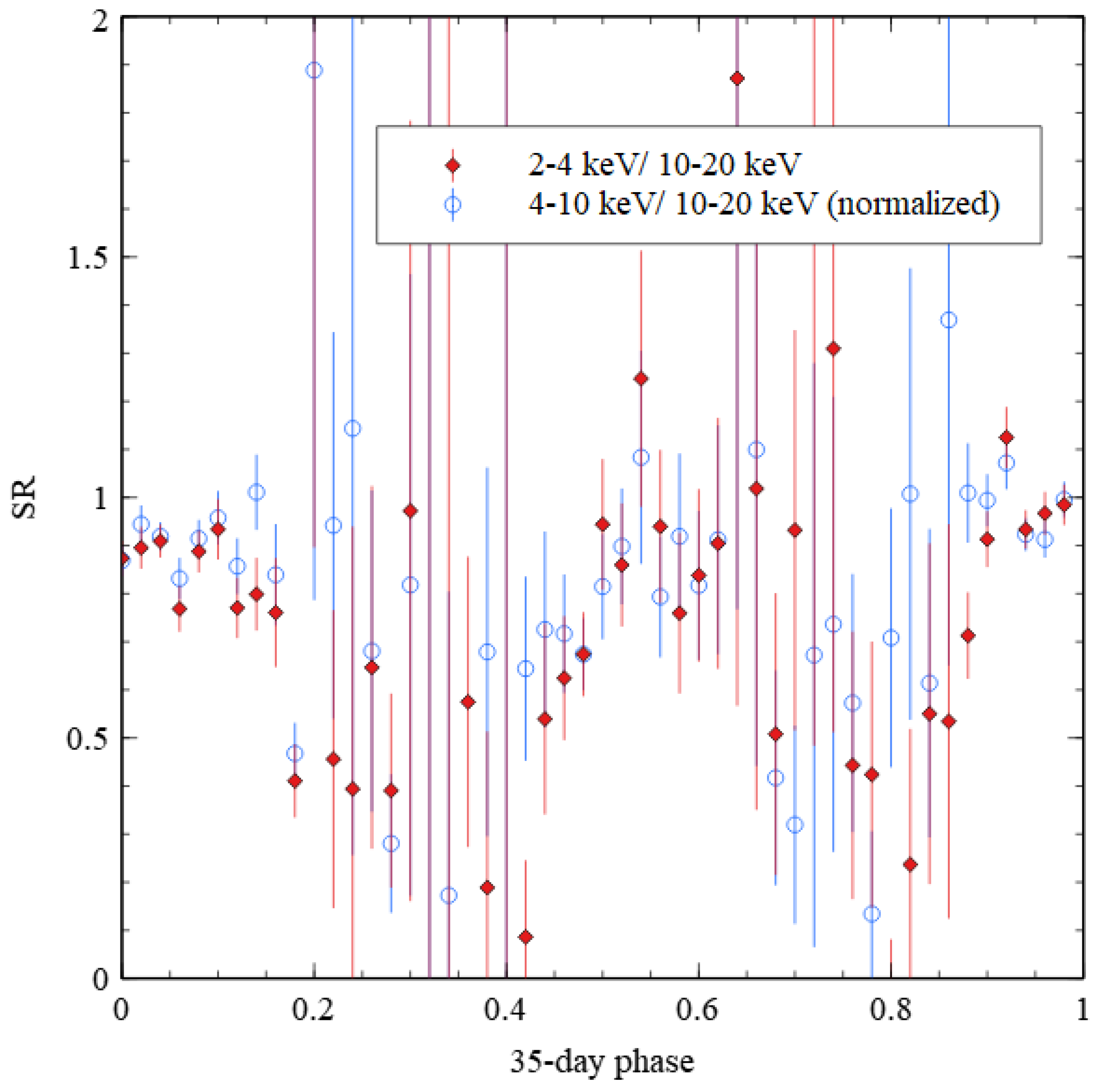
We define the normalized 4–10 keV/10–20 keV SR as the SR multiplied by the ratio of (mean 4–10 keV/10–20 keV SR) to (mean 2–10 keV/10–20 keV SR) for 35-day phase 0.94 to 0.05 (MH excluding TO and decline). This is defined so that it has the same mean value as 2–4 keV/10–20 keV SR over the 35-day phase 0.94 to 0.05, which makes it easy to compare changes in the two SRs. Figure 9 shows a comparison between the 2–4 keV/10–20 keV SR and the normalized 4–10 keV/10–20 keV SR. For TO to MH the 2–4 keV/10–20 keV SR shows lower values compared to 4–10 keV/10–20 keV normalized SR, as expected from absorption by cold matter. Similarly, for SH state TO the 2–4 keV/10–20 keV SR shows lower values than 4–10 keV/10–20 keV normalized SR.
For decline of MH state the 2–4 keV/10–20 keV SR on average shows lower values than 4–10 keV/10–20 keV normalized SR, although for decline the difference between the SRs is of less statistical significance. For SH decline the 2–4 keV/10–20 keV SR and 4–10 keV/10–20 keV normalized SR are not significantly different. Thus, in addition to absorption, scattering and other effects on the spectrum are important for MH and SH decline.
4.3.1. Softness Ratio for MH and SH
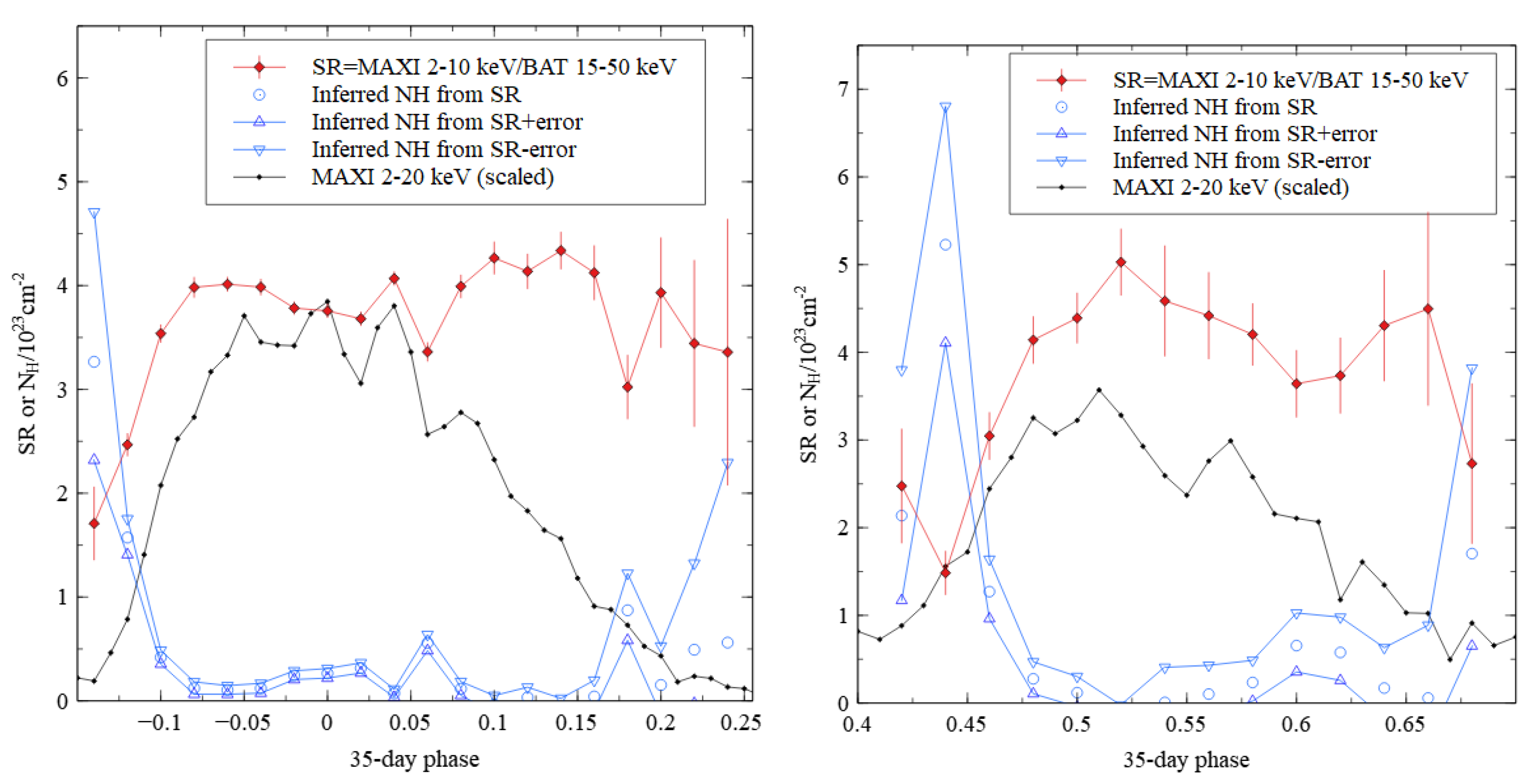
The MAXI 2–10 keV/BAT 15–50 keV SR during MH and SH has significantly smaller errors than the SR for the other bands. Figure 10 shows the MAXI 2–10 keV/BAT 15–50 keV SR with 1 errors during the MH (left panel) and during SH (right panel). To illustrate the flux changes that are simultaneous with the SR changes, we show the MAXI 2–20 keV light-curve scaled to fit on the same plot.
For MH and SH the errors in SR for MAXI 2–10 keV/BAT 15–50 keV are small enough that we can carry out a spectral analysis. In order to determine the effect of absorption on the SR, we model the 2–10 keV MH and SH spectra as described by [14] (their Table 2). For the 15–50 keV states we used the continuum as described by [37] (their Table 3, BPL*HECUT model) for MH, and by [38] (their Table 1) for SH. We then add an extra absorbing column density, , and compute the expected SR. By comparing the expected and measured SR we derive the that fits the data.
The details of the procedure are as follows. The models were fed into the WebPIMMS multiple component model interface,9 which includes the instrument response matrices of MAXI and BAT, to calculate count rates for MAXI 2–4, 4–10, 10–20 and BAT 15–50 keV bands. An additional column density was added to the models. This was repeated for a large number of column densities between and cm. From these absorbed count rates, model SRs were calculated. This produced a SR vs. relation for MH and a different SR vs. relation for SH, because of the different input spectra. Finally, the SR vs. relation for MH was used to produce a vs. 35-day phase plot for MH, and the SR vs. relation for SH was used to produce vs 35-day phase for SH. These are shown in the left and right panels of Figure 10.
For both MH and SH, the radiation from Her X-1 is hardest (smallest SR) when the flux starts to rise at beginning of MH and SH TO (35-day phases ≃−0.14 and 0.44). The radiation softens (SR rises) and column density decreases as TO proceeds for MH and for SH. Then it hardens (SR declines) and column density increases at the end of the decline of MH and of SH. For MH and SH TOs, the softening and decreasing absorption is expected from the outer disk edge moving away from the line-of-sight during TO [23,29]. For MH and SH declines, the flux declines for a ∼4 days (35-day phase 0.06 to ≃0.17 for MH and 0.52 to ≃0.65 for SH) before the rise in column density is detected (at 35-day phase ≃ 0.17 for MH and ≃0.55 to 0.65 for SH).10
The decrease of during SH TO is closely similar to that for MH TO. The for the first point plotted for SH is probably unreliable because the SH spectrum has too large a contribution from the LS spectrum, for which the SR vs. relation from SH is not valid. The increase of during SH decline is also similar to that for MH decline. This is consistent with the standard picture of disk occultation driving the shape of the 35-day cycle ([23,29]).
4.3.2. Softness Ratio for Other 35-Day Phases
For 35-day phases other than MH and SH (e.g., Figure 10), the larger errors imply that SR changes can be detected only by averaging over longer 35-day phase intervals. We chose the ranges in 35-day phase, , given in Table 2 for averaging, omitting MH and SH TOs and declines when SR is changing rapidly. LS1 and LS2 yielded the same results within errors, thus we combined the two. The results are shown in Table 3.
Comparing SH and MH across different energy bands, in all four cases the difference is within . For LS, MAXI 2–4 keV/10–20 keV and 4–10 keV/10–20 keV are lower than for MH by 2.9 and 4.1 respectively. The MAXI 2–10 keV/BAT 15–50 keV and MAXI 2–20 keV/BAT 15–50 keV for LS is not significantly different than for SH or MH.
5. Conclusions
The MAXI and Swift/BAT monitoring data are analyzed here to produce long-term average 35-day cycle light-curves for Her X-1 in different energy bands. The CC methods presented in [22,25] were modified to handle large data gaps, as occur in the MAXI data. The most accurate and complete 35-day cycle timings (peak of MH and cycle lengths) are found using the Swift/BAT data. Thus we use the Swift/BAT timings to construct average 35-day light-curves from MAXI and BAT data.
The 2–20 keV and 15–50 keV 35-day cycle light-curves are quite similar, with main difference that the TO to MH state is later in the 2–20 keV band by 0.343 days. The 2–20 keV/15–50 keV softness ratio shows distinct changes with 35-day phase. These are signatures of the different states of the 35-day cycle: TO to MH, MH, decline of MH, LS 1, TO to SH, decline of SH and LS 2. In addition, the light-curves and softness ratios reveal recurrent broad absorption dips during MH and SH states (Figure 8).
Average 35-day light-curves were constructed for the 2–4 keV, 4–10 keV, 10–20 keV sub-bands of MAXI. From these, softness ratios in narrower energy bands were calculated which are more sensitive to spectral changes, especially column density, than the broad-band softness ratio. Spectral modelling was used to extract column density vs. 35-day phase for MH and SH states (Figure 10). The column density drops simultaneously with the flux rise for TO of both states. This is consistent with decreasing cold-matter absorption at TO from the outer disk edge moving out of the line-of-sight [29]. The flux decline starts much earlier than the column density rise for decline of both states, consistent with optically thick obscuration by the inner disk edge [2]. The column density for MH and for SH shows nearly the same behaviour, consistent with accretion disk occultation model for the 35-day cycle, where both MH and SH TOs are caused by the outer disk edge and the declines of both states are caused by the inner disk edge.
In summary, the average 35-day light-curve has now been well-characterized in multiple energy bands. The mean durations of the states of the 35-day cycle are better measured than previously (Table 2). A number of features which were previously only detected in individual observations at higher sensitivity are now measured in the long-term average 35-day light-curve. This illustrates that the accretion disk in Hercules X-1 has been quite stable over the past ∼10 years, despite a small amount of variability in 35-day X-ray cycle lengths and amplitude. It has been stable likely since Her X-1 was first discovered in the 1970’s,11 with the notable exception of disk changes during intermittent ALSs.
The long-term average light-curves and softness ratios will be an important input for modelling the binary system, which now must include the scattering material and the accretion stream [39] in addition to the existing model structures [29]: neutron star, companion star and warped precessing accretion disk. In particular, the new 35-day light-curves can be used to significantly improve the physical binary system models by providing new constraints on the different components in the system.
Author Contributions
Conceptualization, D.L.; methodology, D.L.; software, Y.W.; validation, D.L., Y.W.; writing—original draft preparation, Y.W.; writing—review and editing, D.L.; supervision, D.L.; project administration, D.L.; funding acquisition, D.L. All authors have read and agreed to the published version of the manuscript.
Funding
This research was funded by Natural Sciences and Engineering Research Council of Canada.
Data Availability Statement
This research has made use of MAXI data provided by RIKEN, JAXA and the MAXI team. The data were accessed on 19 June 2020. The MAXI data products are available at the website http://maxi.riken.jp/pubdata/v7l/. The Swift/BAT data are available at the website https://swift.gsfc.nasa.gov/results/transients/.
Conflicts of Interest
The authors declare no conflict of interest.
Abbreviations
The following abbreviations are used in this manuscript:
| CC | cross correlation |
| UV | Ultraviolet |
| EUV | Extreme Ultraviolet |
| MAXI | Monitoring All-Sky X-Ray Images |
| BAT | Burst Alert Telescope |
| RXTE | Rossi X-ray Timing Explorer |
| ASM | All Sky Monitor |
| PCA | Proportional Counter Array |
| MJD | Modified Julian Date |
| MH | Main High |
| SH | Short High |
| LS | Low State |
| ALS | Anomalous Low State |
| TO | Turn On |
Appendix A. Modified Cross-Correlation (CC) Method for MAXI Data
The weighted CC function is defined as previously:
where is observed count rate, is template value, is count rate error and the weight is . In the modified CC method, we select one full 35-day cycle of data as follows:12 Given a data point at MJD time ,
- At , calculate and days, assuming a initial 35-day cycle length of . Select data between and (total points).
- For all observed points () in this cycle, convert time (MJD) to 35-day phases with .
- With the list , find corresponding template count rates at using cubic interpolation on the input template.
- Calculate with Equation (A1) from the set of constructed for each .
To avoid having the 35-day cycle analysis affected by aliasing with the 1.7 day orbital period, we remove data from times of eclipse (orbital phase 0.93 to 1.07). We remove extra time on either side of eclipse because that is the time period when dips are concentrated [30]. Thus we kept data with orbital phases of 0.16–0.84 (boundaries inclusive), which contribute ∼68.1% of the original data in MAXI. The 10,180 in-eclipse data points were replaced by simulated data. The simulated data were calculated by linear interpolation between the corresponding edge points with orbital phases ≃0.16 and ≃0.84, followed by adding fluctuations from a Gaussian distribution, with standard deviation based on the sum errors of the edge points. New rate errors are also assigned to be errors from the two edges summed. As a result, the number of data points and the time of observation are retained, and we are able to study the properties of the 35-day cycle without data gaps during eclipses.
We assumed an initial 35-day cycle length, to adapt to the large data gaps in MAXI and obtain the initial 35-day phase calculation of all data points. After each iteration of the CC method, the variable 35-day cycle lengths were then re-calculated from MH peak times, and the variable cycle lengths were used in calculating a better 35-day average light-curve.
Appendix B. Calculation of Average 35-Day Light-Curve with Reference MH Peak Times
The following procedure creates average 35-day light-curves with an input list of reference MH peak times (35-day phase 0 times).
- Calculate 35-day cycle lengths using reference phase 0 times (MJD) for all cycles. Calculate phase for all data points.
- Split into N bins. We use bins for 35-day cycle light-curve, and reduce to bins for calculating softness ratios, to obtain smaller error bars. For the kth bin: , i points fall in this bin.
- In the kth bin, calculate the average rate and standard deviation given by .
- Estimate the error for this bin:
| 1. | http://maxi.riken.jp/star_data/J1657+353/J1657+353.html. The data were accessed on 19 June 2020. |
| 2. | For this analysis we assumed a fixed 35-day cycle length of 35 days to calculate only for simplicity. For the final 35-day light-curve of MAXI we used a variable 35-day cycle length to calculate and our final method described in Section 2.2.3 uses that. |
| 3. | We use the mean , and sample standard deviation with the data points and n the number of data points. |
| 4. | The published paper contains only the first 10 lines: the complete table is published as online Table 1 of [25]. |
| 5. | In Section 4.2.1 below we introduce an improved definition of start of TO. |
| 6. | |
| 7. | Dips are a separate phenomena, require a separate explanation from the disk occultation model, and are discussed below. |
| 8. | Table 2 gives the error in absolute 35-day phase which is ≃, limited by the bin size. The error in difference in 35-day phase between MAXI and BAT is limited by the observation intervals (∼60 s for MAXI and ∼1000 s for BAT, yielding a net 35-day phase uncertainty of ). The CC analysis yielded a time difference between MAXI and BAT of 0.343 days with an error of 0.157 days, which corresponds to an uncertainty of 0.0045 in 35-day phase. |
| 9. | Available online: https://heasarc.gsfc.nasa.gov/cgi-bin/Tools/w3pimms/w3pimms.pl, accessed on 26 April 2021. |
| 10. | The errors in SR and inferred column density are large enough for SH, so it is not clear when the rise in column density during SH decline occurs. We can only say that it is between 35-day phases 0.55 to 0.65. |
| 11. | |
| 12. | Compared to the CC method used for Swift/BAT and RXTE/ASM in [25], and in the new method are not required to be in the data set. |
References
- Giacconi, R.; Gursky, H.; Kellogg, E.; Levinson, R.; Schreier, E.; Tananbaum, H. Further X-ray observations of Hercules X-1 from Uhuru. Astrophys. J. 1973, 184, 227–236. [Google Scholar] [CrossRef]
- Scott, D.M.; Leahy, D.A.; Wilson, R.B. The 35 Day Evolution of the Hercules X-1 Pulse Profile: Evidence for a Resolved Inner Disk Occultation of the Neutron Star. Astrophys. J. 2000, 539, 392–412. [Google Scholar] [CrossRef] [Green Version]
- Staubert, R.; Klochkov, D.; Vasco, D.; Postnov, K.; Shakura, N.; Wilms, J.; Rothschild, R.E. Variable pulse profiles of Hercules X-1 repeating with the same irregular 35 d clock as the turn-ons. Astron. Astrophys. 2013, 550, 110–118. [Google Scholar] [CrossRef] [Green Version]
- Petterson, J.A. Hercules X-1: A neutron star with a twisted accretion disk? Astrophys. J. 1975, 201, L61–L64. [Google Scholar] [CrossRef]
- Gerend, D.; Boynton, P.E. Optical clues to the nature of Hercules X-1/HZ Herculis. Astrophys. J. 1976, 209, 562–573. [Google Scholar] [CrossRef]
- Parmar, A.N.; Pietsch, W.; McKechnie, S.; White, N.E.; Truemper, J.; Voges, W.; Barr, P. An extended X-ray low state from Hercules X-1. Nature 1985, 313, 119–121. [Google Scholar] [CrossRef]
- Delgado, A.J.; Schmidt, H.U.; Thomas, H.-C. HZ Herculis, still active. Astrophys. J. 1983, 127, L15–L16. [Google Scholar]
- Coburn, W.; Heindl, W.A.; Wilms, J.; Gruber, D.E.; Staubert, R.; Rothschild, R.E.; Pelling, M.R.; Risse, P. The 1999 Hercules X-1 Anomalous Low State. Astrophys. J. 2000, 543, 351–358. [Google Scholar] [CrossRef] [Green Version]
- Leahy, D.A.; Dupuis, J. Extreme Ultraviolet Explorer Observations of Hercules X-1 over a 35 Day Cycle. Astrophys. J. 2010, 715, 897–901. [Google Scholar] [CrossRef] [Green Version]
- Leahy, D.A. GINGA observations of absorption dips in Hercules X-1. Mon. Not. R. Astron. Soc. 1997, 287, 622–628. [Google Scholar] [CrossRef] [Green Version]
- Choi, C.S.; Seon, K.I.; Dotani, T.; Nagase, F. A Low State Eclipse Spectrum of Hercules X-1 Observed with ASCA. Astrophys. J. 1997, 476, L81–L84. [Google Scholar] [CrossRef] [Green Version]
- dal Fiume, D.; Orlandini, M.; Cusumano, G.; Del Sordo, S.; Oosterbroek, T.; Cusumano, G.; Parmar, A.N.; Santangelo, A.; Feroci, M.; Frontera, F.; et al. The broad-band (0.1-200 keV) spectrum of HER X-1 observed with BeppoSAX. Astron. Astrophys. 1998, 329, L41–L44. [Google Scholar]
- Oosterbroek, T.; Parmar, A.N.; Martin, D.D.E.; Lammers, U. The BeppoSAX LECS X-ray spectrum of Hercules X-1. Astron. Astrophys. 1997, 327, 215–218. [Google Scholar]
- Leahy, D.A.; Chen, Y. AstroSat SXT Observations of Her X-1. Astrophys. J. 2019, 871, 152–161. [Google Scholar] [CrossRef]
- Boroson, B.; Blair, W.P.; Davidsen, A.F.; Vrtilek, S.D.; Raymond, J.; Long, K.S.; McCray, R. Hopkins Ultraviolet Telescope Observations of Hercules X-1. Astrophys. J. 1997, 491, 903–909. [Google Scholar] [CrossRef] [Green Version]
- Vrtilek, S.D.; Cheng, F.H. The Ultraviolet/Optical Continuum of Hercules X-1/HZ Herculis. Astrophys. J. 1996, 465, 915–922. [Google Scholar] [CrossRef]
- Leahy, D.A.; Marshall, H.; Scott, D.M. EUVE Observations of Hercules X-1 during a Short High-State Turn-on. Astrophys. J. 2000, 542, 446–453. [Google Scholar] [CrossRef] [Green Version]
- Deeter, J.; Crosa, L.; Gerend, D.; Boynton, P.E. Analysis of periodic optical variability in the compact X-ray source Her X-1/HZ Herculis. Astrophys. J. 1976, 206, 861–868. [Google Scholar] [CrossRef]
- Voloshina, I.B.; Lyutyi, V.M.; Sheffer, E.K. Some Characteristics of the Photometric Behavior of Hz-Herculis HERCULES-X-1—The Effect of the Twisted Disk. Sov. Astron. Lett. 1990, 16, 267–270. [Google Scholar]
- Anderson, S.F.; Wachter, S.; Margon, B.; Downes, R.A.; Blair, W.P.; Halpern, J.P. Ultraviolet Spectra of HZ Herculis/Hercules X-1 from HST: Hot Gas during Total Eclipse of the Neutron Star. Astrophys. J. 1994, 436, 319–325. [Google Scholar] [CrossRef]
- Leahy, D.A.; Abdallah, M.H. HZ Her: Stellar Radius from X-Ray Eclipse Observations, Evolutionary State, and a New Distance. Astrophys. J. 2014, 793, 79–86. [Google Scholar] [CrossRef] [Green Version]
- Leahy, D.A.; Igna, C.D. RXTE-based 35 Day Cycle Turn-on Times for Hercules X-1. Astrophys. J. 2010, 713, 318–324. [Google Scholar] [CrossRef] [Green Version]
- Scott, D.M.; Leahy, D.A. Rossi X-Ray Timing Explorer All-Sky Monitor Observations of the 35 Day Cycle of Hercules X-1. Astrophys. J. 1999, 510, 974–985. [Google Scholar] [CrossRef]
- Shakura, N.I.; Ketsaris, N.A.; Prokhorov, M.E.; Postnov, K.A. RXTE highlights of the 34.85-day cycle of HER X-1. Mon. Not. R. Astron. Soc. 1998, 300, 992–998. [Google Scholar] [CrossRef] [Green Version]
- Leahy, D.; Wang, Y. Swift/BAT and RXTE/ASM Observations of the 35 day X-Ray Cycle of Hercules X-1. Astrophys. J. 2020, 902, 146–154. [Google Scholar] [CrossRef]
- Matsuoka, M.; Kawasaki, K.; Ueno, S.; Tomida, H.; Kohama, M.; Suzuki, M.; Ebisawa, K. The MAXI Mission on the ISS: Science and Instruments for Monitoring All-Sky X-Ray Images. Publ. Astron. Soc. Jpn. 2009, 61, 999–1010. [Google Scholar] [CrossRef]
- Krimm, H.A.; Holland, S.T.; Corbet, R.H.D.; Pearlman, A.B.; Romano, P.; Kennea, J.A.; Ukwatta, T.N. The Swift/BAT Hard X-Ray Transient Monitor. Astrophys. J. Suppl. Ser. 2013, 209, 14–46. [Google Scholar] [CrossRef] [Green Version]
- Kuster, M.; Wilms, J.; Staubert, R.; Heindl, W.A.; Rothschild, R.E.; Shakura, N.I.; Postnov, K.A. Probing the outer edge of an accretion disk: A Her X-1 turn-on observed with RXTE. Astron. Astrophys. 2005, 443, 753–767. [Google Scholar] [CrossRef] [Green Version]
- Leahy, D.A. Modelling RXTE/ASM observations of the 35-d cycle in Her X-1. Mon. Not. R. Astron. Soc. 2002, 334, 847–854. [Google Scholar] [CrossRef]
- Leahy, D.A.; Igna, C. The Light Curve of Hercules X-1 as Observed by the Rossi X-Ray Timing Explorer. Astrophys. J. 2011, 736, 74–80. [Google Scholar] [CrossRef]
- Wijers, R.A.M.J.; Pringle, J.E. Warped accretion discs and the long periods in X-ray binaries. Mon. Not. R. Astron. Soc. 1999, 308, 207–220. [Google Scholar] [CrossRef] [Green Version]
- Leahy, D.A. Observations of spectral shape changes in Hercules X-1. Astron. Astrophys. Suppl. Ser. 1995, 113, 21–31. [Google Scholar]
- Igna, C.D.; Leahy, D.A. Hercules X-1’s light-curve dips as seen by the RXTE/PCA: A study of the entire 1996 February–2005 August light-curve. Mon. Not. R. Astron. Soc. 2011, 418, 2283–2291. [Google Scholar] [CrossRef] [Green Version]
- Leahy, D.A.; Yoshida, A.; Matsuoka, M. Spectral Evolution during Pre-Eclipse Dips in Hercules X-1. Astrophys. J. 1994, 434, 341–347. [Google Scholar] [CrossRef]
- Reynolds, A.P.; Parmar, A.N. A comparison between the Hercules X-1 pre-eclipse and anomalous dips. Astron. Astrophys. 1995, 297, 747–753. [Google Scholar]
- Leahy, D.A.; Chen, Y. Results from AstroSat LAXPC Observations of Hercules X-1 (Her X-1). arXiv 2021, arXiv:2012.02736. [Google Scholar]
- Asami, F.; Enoto, T.; Iwakiri, W.; Yamada, S.Y.; Tamagawa, T.; Mihara, T.; Nagase, F. Broad-band spectroscopy of Hercules X-1 with Suzaku. Publ. Astron. Soc. Jpn. 2014, 66, 44. [Google Scholar] [CrossRef] [Green Version]
- Abdallah, M.H.; Leahy, D.A. Spectral signature of atmospheric reflection in Hercules X-1/HZ Hercules during low and short high states. Mon. Not. R. Astron. Soc. 2015, 4, 4222–4231. [Google Scholar]
- Igna, C.D.; Leahy, D.A. Light-curve dip production through accretion stream-accretion disc impact in the HZ Her/Her X-1 binary star system. Mon. Not. R. Astron. Soc. 2012, 425, 8–20. [Google Scholar] [CrossRef] [Green Version]
Figure 1.
Two examples of 35-day cycles in MAXI data (red dots and solid lines) and Swift/BAT data (blue crosses and dotted lines). The BAT cycle numbers (80 and 97) from [25] are shown in top and bottom panel, respectively. The vertical lines near peak of Main High (MH) show the CC-detected MH peak times: the red line for the MAXI data and the blue line for the BAT data.

Figure 2.
Top panel: ∼300 day section of MAXI 2–20 keV data illustrating data gaps; bottom panel CC function from the final iteration of the CC method. The MH peaks found using peaks in the CC function are marked with vertical black lines. The top panel shows count rate (cts/sec/cm) vs MJD time. The bottom panel shows CC values vs MJD time. The black vertical lines indicate CC peaks, which align with MH peaks.

Figure 3.
Swift/BAT average 35-day light-curve with standard deviation (SD) and error compared with previous results in [25]. The red solid line with errorbar shows the new 100-bin light-curve of Swift/BAT with SD the black crosses dotted line, and the blue dashed line shows the previous light-curve with SD the yellow triangles on dotted line.

Figure 4.
Histogram of time differences dt between MAXI and BAT MH peak times for MH peaks detected in both sets of data. The best fit Gaussian distribution, excluding the 2 outlier bins, is shown by the line, and has mean 0.36 days, and 1 width of 0.74 days.
Figure 4.
Histogram of time differences dt between MAXI and BAT MH peak times for MH peaks detected in both sets of data. The best fit Gaussian distribution, excluding the 2 outlier bins, is shown by the line, and has mean 0.36 days, and 1 width of 0.74 days.

Figure 5.
Top panel: MAXI average 35-day light-curve (Template) with SD and error compared with Swift/BAT average 35-day light-curve. The blue dashed line with error bars shows the new 100-bin light-curve of MAXI 2–20 keV with SD the yellow triangles, and the red solid line with error bars shows the Swift/BAT light-curve with SD the black crosses. Bottom panel: the difference in normalized MAXI count rate and normalized BAT count rate vs. 35 day phase, showing the significance of the difference during MH TO (35-day phase ≃−0.13 to −0.05), during SH TO (35-day phase ≃0.44 to 0.49), and during the major MH dips (35-day phases ≃–0.02, 0.02 and 0.06).

Figure 6.
MAXI average 35-day light-curves and softness ratios (SR) vs. 35 day phase for different energy bands. The red solid lines with cross symbols show the light-curves created using BAT MH peak times for MAXI energy bands, and the blue dashed lines with circle symbols show SR vs. 35-day phase. (a) Total (2–20 keV) light-curve with = MAXI Band 1 (2–4 keV) and = MAXI Band 3 (10–20 keV); (b) Band 1 (2–4 keV) light-curve with = MAXI Band 2 (4–10 keV) and = MAXI Band 3 (10–20 keV); (c) Band 2 (4–10 keV) light-curve with = MAXI Band 1 + 2 (2–10 keV) and = Swift/BAT (15–50 keV); and (d) Band 3 (10–20 keV) light-curve with = MAXI (2–20 keV) and = Swift/BAT (15–50 keV).

Figure 7.
Orbital phase distributions of peak of MH. Top panel: from MAXI CC analysis, with Gaussian plus uniform fit; bottom panel: from Swift/BAT CC analysis with Gaussian plus uniform fit.
Figure 7.
Orbital phase distributions of peak of MH. Top panel: from MAXI CC analysis, with Gaussian plus uniform fit; bottom panel: from Swift/BAT CC analysis with Gaussian plus uniform fit.

Figure 8.
Average 35-day light-curve for MAXI 2–20 keV band (blue line), with 2–20 keV/15–50 keV softness ratio (SR, red points with error bars). The vertical black lines mark the minima in SR during the MH state (MH d1, MH d2 and MH d3) and during SH state (SH d1 and SH d2). The minima in SR match the local minima in the MAXI 2–20 keV light-curve in all cases, illustrating that the dips are consistent with absorption as the cause.

Figure 9.
MAXI 2–4 keV/10–20 keV Softness Ratio (SR, red symbols with 1 errors) compared to MAXI 4–10 keV/10–20 keV normalized SR (blue symbols with 1 errors).
Figure 9.
MAXI 2–4 keV/10–20 keV Softness Ratio (SR, red symbols with 1 errors) compared to MAXI 4–10 keV/10–20 keV normalized SR (blue symbols with 1 errors).

Figure 10.
MAXI 2–10 keV/BAT 15–50 keV Softness Ratio (SR, red symbols with 1 errors) during the MH (left panel) and during the SH (right panel) portions of 35-day phase. The inferred from spectral modelling of the SR (see text for details) is shown by the open blue circles, with upper and lower limits on shown by the blue lines and blue triangles. The scaled MAXI 2–20 keV light-curve is shown in black for comparison.


Table 1.
Mean MAXI and BAT countrates for different 35-day states.
| Instrument | State | Mean | Error |
|---|---|---|---|
| MAXI 2–20 keV | MH | 0.3500 | 0.0029 |
| SH | 0.0822 | 0.0036 | |
| LS | 0.0154 | 0.0010 | |
| BAT 15–50 keV | MH | 0.05498 | 0.00026 |
| SH | 0.01166 | 0.00037 | |
| LS | 0.00210 | 0.00013 |
Table 2.
35-day phases of the 35-day states .
| State | Start Phase (Error) | End Phase (Error) | Duration (Error) |
|---|---|---|---|
| Main High Turn-On | 0.865 (0.01) | 0.945 (0.01) | 0.08 (0.015) |
| Main High | 0.945 (0.01) | 0.055 (0.01) | 0.11 (0.015) |
| Main High decline | 0.055 (0.01) | 0.25 (0.02) | 0.195 (0.022) |
| Low State 1 | 0.25 (0.02) | 0.435 (0.01) | 0.185 (0.022) |
| Short High Turn-On | 0.435 (0.01) | 0.485 (0.01) | 0.05 (0.015) |
| Short High | 0.485 (0.01) | 0.515 (0.01) | 0.03 (0.015) |
| Short High decline | 0.515 (0.01) | 0.71 (0.02) | 0.195 (0.022) |
| Low State 2 | 0.71 (0.02) | 0.865 (0.01) | 0.155 (0.022) |
1: 35-day phase 0 is defined by peak of MH state.
Table 3.
Average softness ratios for different 35-day states.
| State | Mean | Error | SD | ||
|---|---|---|---|---|---|
| MAXI 2–4 keV | MAXI 10–20 keV | MH | 0.90695 | 0.040292 | 0.066322 |
| SH | 0.81774 | 0.13156 | 0.16907 | ||
| LS | 0.34696 | 0.18948 | 1.0592 | ||
| MAXI 4–10 keV | MAXI 10–20 keV | MH | 1.3334 | 0.051164 | 0.070918 |
| SH | 1.1542 | 0.16548 | 0.17252 | ||
| LS | 0.38835 | 0.22735 | 1.2616 | ||
| MAXI 2–10 keV | BAT 15–50 keV | MH | 3.8295 | 0.071815 | 0.22697 |
| SH | 4.2979 | 0.35010 | 0.39458 | ||
| LS | 3.4399 | 1.5884 | 5.0666 | ||
| MAXI 2–20 keV | BAT 15–50 keV | MH | 6.2366 | 0.10947 | 0.29360 |
| SH | 7.1769 | 0.57374 | 0.62307 | ||
| LS | 7.1742 | 2.8254 | 10.660 |
Publisher’s Note: MDPI stays neutral with regard to jurisdictional claims in published maps and institutional affiliations. |
© 2021 by the authors. Licensee MDPI, Basel, Switzerland. This article is an open access article distributed under the terms and conditions of the Creative Commons Attribution (CC BY) license (https://creativecommons.org/licenses/by/4.0/).
Share and Cite
MDPI and ACS Style
Leahy, D.; Wang, Y. The 35-Day Cycle of Hercules X-1 in Multiple Energy Bands from MAXI and Swift/BAT Monitoring. Universe 2021, 7, 160. https://doi.org/10.3390/universe7060160
AMA Style
Leahy D, Wang Y. The 35-Day Cycle of Hercules X-1 in Multiple Energy Bands from MAXI and Swift/BAT Monitoring. Universe. 2021; 7(6):160. https://doi.org/10.3390/universe7060160
Chicago/Turabian StyleLeahy, Denis, and Yuyang Wang. 2021. "The 35-Day Cycle of Hercules X-1 in Multiple Energy Bands from MAXI and Swift/BAT Monitoring" Universe 7, no. 6: 160. https://doi.org/10.3390/universe7060160
Note that from the first issue of 2016, this journal uses article numbers instead of page numbers. See further details here.