
Inclusion of Narrow Flow Paths between Buildings in Coarser Grids for Urban Flood Modeling: Virtual Surface Links


1
Department of Civil, Geo and Environmental Engineering, Technical University of Munich, Arcisstrasse 21, 80333 Munich, Germany
2
Research Institute of Water and Environment, University of Siegen, Paul-Bonatz-Strasse 9-11, 57076 Siegen, Germany
*
Author to whom correspondence should be addressed.
Water 2021, 13(19), 2629; https://doi.org/10.3390/w13192629
Submission received: 12 August 2021
/
Revised: 21 September 2021
/
Accepted: 22 September 2021
/
Published: 24 September 2021
(This article belongs to the Special Issue Urban Flood Model Developments and Flood Forecasting)
Abstract
:Urban flood modeling benefits from new remote sensing technologies, which provide high-resolution data and allow the consideration of small-scale urban key features. Since high-resolution data often result in large simulation runtimes, coarsening of the 2D grid via resampling techniques can be used to achieve a good balance between accuracy and computation time. However, the representation of urban features and topographical properties degrades, since small-scale features are blurred. Therefore, narrow flow paths between buildings are often not considered, building’s sizes are overestimated, and their arrangement in the grid changes. Thus, flow paths change and waterways are blocked, leading to incorrect inundations around buildings. This paper develops a method to improve the simulation results of coarser grids by adding virtual surface links (VSL) between buildings. The VSL mimic the flow paths of a high-resolution model in the areas of interest. The approach is developed for dual-drainage 1D/2D models. The approach shows a visible improvement at the localized level where the VSL are applied, in terms of under/overestimating flooding and a moderate overall improvement of the simulation results. Relatively to the model resolution of 2 m, the computational time, by applying this method, is reduced by 93.6% when using a 5 m grid and by 99% when using a 10 m grid. For a small test case, where the local effects are investigated, the error in the maximum water volume, relative to a grid size of 2 m, is reduced from 69.63% to 5.03% by using a 5 m grid and from 152.75% to 22.92% for a 10 m grid.
1. Introduction
Flash floods, resulting from heavy rainfall events, constitute a serious risk to urban areas [1]. The recent events of 14 July 2021, in Germany and Belgium, remind us that this is a global threat that is not limited to developing countries. Urban areas are characterized by a heterogeneous area, which influences the flow routing. The flood extent is significantly affected by the underground and surface drainage systems, as well as other key urban features [2]. Buildings, in particular, affect the flow path of water, and thus the flood inundation [3]. By means of new technologies, such as light detection and ranging (LiDAR), small-scale features can be better considered in flood models, and enable a more accurate simulation [4]. The complex interaction of the water flow with the surrounding leads to a great variation in the flood dynamics in space and time. Additionally, local changes in flow regimes result in complex flow characteristics [5]. One-dimensional models, which benefit from a fast simulation runtime, are insufficient for representing complex topographies, because of their limitations in representing 2D flood routing [6]. Hence, 2D hydraulic models and high-resolution data are necessary for an accurate representation of urban key features and 2D flood routing. As a consequence, the computation time increases, often leading to unreasonable runtimes [7]. Hence, a compromise between computation time and accuracy is required. Established resampling techniques, such as nearest, bilinear, or cubic, can be used to coarsen the digital terrain model (DTM) resolution and reduce the runtime [8]. In resampling, the grid values of a finer grid are interpolated to generate a new raster dataset with a different resolution. This approach leads to an undesired degradation in the representation of urban features, including the shape, location, and elevation of such features [9]. Buildings often lead to an overestimation of the flood depths, due to a larger blockage effect of the routes for flooding [10]. Resampling may lead to the merging of close buildings, whereby narrow flow paths between buildings may disappear. The opposite can also occur if small buildings are suddenly removed due to the coarsening of the grid [11]. Subsequently, flow routing processes are significantly changed, affecting the local and temporal pattern of the flow [12]. Moreover, coarsening the grid has a large influence on the depiction of the topography. Resampling techniques reduce the heterogeneity and complexity of the topography, resulting in a change in the flood wave travel time and the spatial distribution of potential floodplains [7,12].
Research regarding a good balance between precision and model runtime, and improvements in the representation of urban features have been the focus of recent researchers. The recommended mesh size for urban areas varies depending on the study area and the aim. While Maksimovic and Prodanovic suggest a mesh size of 1–2 m [13], Mark, Weesakul, Apirumanekul, Aroonnet, and Djordjević recommend a range of 1–5 m [14]. Parallelization methods, through the use of multiple cores, can reduce the computational time significantly [15]. Several GPU-based parallel algorithms have been developed, which enable large-scale simulation using the full St. Venant equation and high-resolution data [16]. Besides parallelization methods, different mesh design approaches have been developed to speed up the computation time, with reducing deterioration in the overall accuracy. A common method constitutes the adaptive mesh refinement method (AMR). The mesh is refined locally, where high-resolution data are necessary [17]. Another procedure constitutes the active-cell method and the multigrid method. The first method speeds up the computational time by focusing on the areas that are affected by inundation, whereas the multigrid method divides the area into several grids with different resolutions. These grids are classified into the main grid, and upstream and downstream extended grids. To speed up the calculations, the extended grids are simulated with a lower resolution [18]. However, these methods show a limited improvement in the computational time, since finer resolutions are still required for the relevant areas, and those are the ones responsible for very small computational time steps, bounded by the Courant number (or accuracy restrictions in the case of implicit schemes). Another alternative approach is to preserve the fine terrain details by including them in coarser models. In this case, the 2D calculations depend on constructing linear data tables for the accurate non-linear interpolation of the instantaneous volume stored in a cell and the corresponding surface area, taking into account the detailed terrain geometry (e.g., [19]). Another method to represent small-scale features in coarser grids more accurately constitutes porosity models. Porosity models aim to keep the computational benefits of coarse grids, by including the overall impact of smaller-scale effects, through the use of porosity parameters [20]. These approaches, however, may not allow complex independent paths that may exist between buildings to be described. These may be responsible for the transfer of discharge across two coarse grid cells that may not necessarily share common cell boundaries.
This paper introduces a methodology that is applicable to 1D/2D dual-drainage models with a regular grid, for improving the simulation results for coarser grids, while benefiting from faster simulation times. One-dimensional/two-dimensional dual-drainage models are the state-of-the-art tool for the simulation of floods in urban areas. Here, a 1D sewer network model (minor system) is coupled with a 2D overland flow model (major system) for simulating the bi-directional interaction between the major and the minor system. This allows for a more precise simulation, by considering the retention capacity of the sewer system, as well as the surcharge and drainage flow from and to the drainage system [21]. Since the accurate representation of the flow around the buildings is one of the most important aspects for an accurate flood simulation in urban areas, this new approach focuses on improving the flow routing of narrow flow paths between buildings in coarser grids. Herein, the concept of virtual surface links (VSL) is developed with the aim of mimicking high-resolution flow paths in a coarser 2D model. As such, narrow flow paths can be explicitly included in the simulation while keeping the efficient computational time of coarser grids. A detailed description of the new approach, the validation procedure, and applied models are presented in Section 2. Section 3 shows the results and provides an overview of the effectiveness of the new approach. The results are evaluated in the Discussion section, and the final section summarizes and concludes the work.
2. Materials and Methods
This approach focuses on the narrow flow paths around buildings. Since resampling techniques change the topographic properties and representations of buildings, the flow routing is altered in urban areas. This study assumes that high-resolution meshes provide a more accurate representation of small-scale features and thus a better prediction of flow routing and flood inundation extent [12]. Buildings are considered by the building blocking (BB) method, whereas the ground elevation is increased by the height of the buildings [22]. The validation follows a two-stage procedure. The first is conducted for a very small area for testing, and the second larger area is for final validation.
2.1. Virtual Surface Links (VSL) Principle and Setup
The principle of the virtual surface links (VSL) approach is to mimic the overland flow of high-resolution meshes. One-dimensional virtual links are added to the 1D/2D dual-drainage flow model, similarly to conduits of a sewer network model. The VSL represent the narrow flow paths around buildings, obtained from a high-resolution mesh. The high-resolution flow paths around buildings are determined by an automatic delineation of the 1D overland flow based on the fine mesh. VSL focus on the simulation around (or between) buildings, correcting water accumulations due to missing small-scale waterways, and incorrect representations of buildings. Since this concept requires a 1D model for simulating the VSL, a 2D overland flow model for representing the bi-dimensional flow surface and an exchange module for capturing the bi-directional interaction between the two, it is more suitable to implement directly in 1D/2D dual-drainage models. By allowing a bi-directional flow, backwater effects and reverse flow can be considered. The dual-drainage model allows the flow to be calculated, and the exchange between the two models for each time step, at the correct time and without continuity losses [23]. A detailed mathematical description of the flow equations and the coupling process is given in Section 2.4. The advantages of the VSL concept are that high-resolution flow paths can be included by only increasing the computational time marginally. Since most of the area is simulated in 2D, the VSL method ensures an accurate flow simulation by reducing incorrect backwater effects close to urban features (e.g., buildings, etc.) due to coarsening. Also, complex flow paths that may connect non-neighboring cells are kept as the VSL method alone defines the entry and exit points. Lastly, this approach benefits from an easy and fast implementation by means of automatic delineation, which only needs to be defined in the areas of interest.
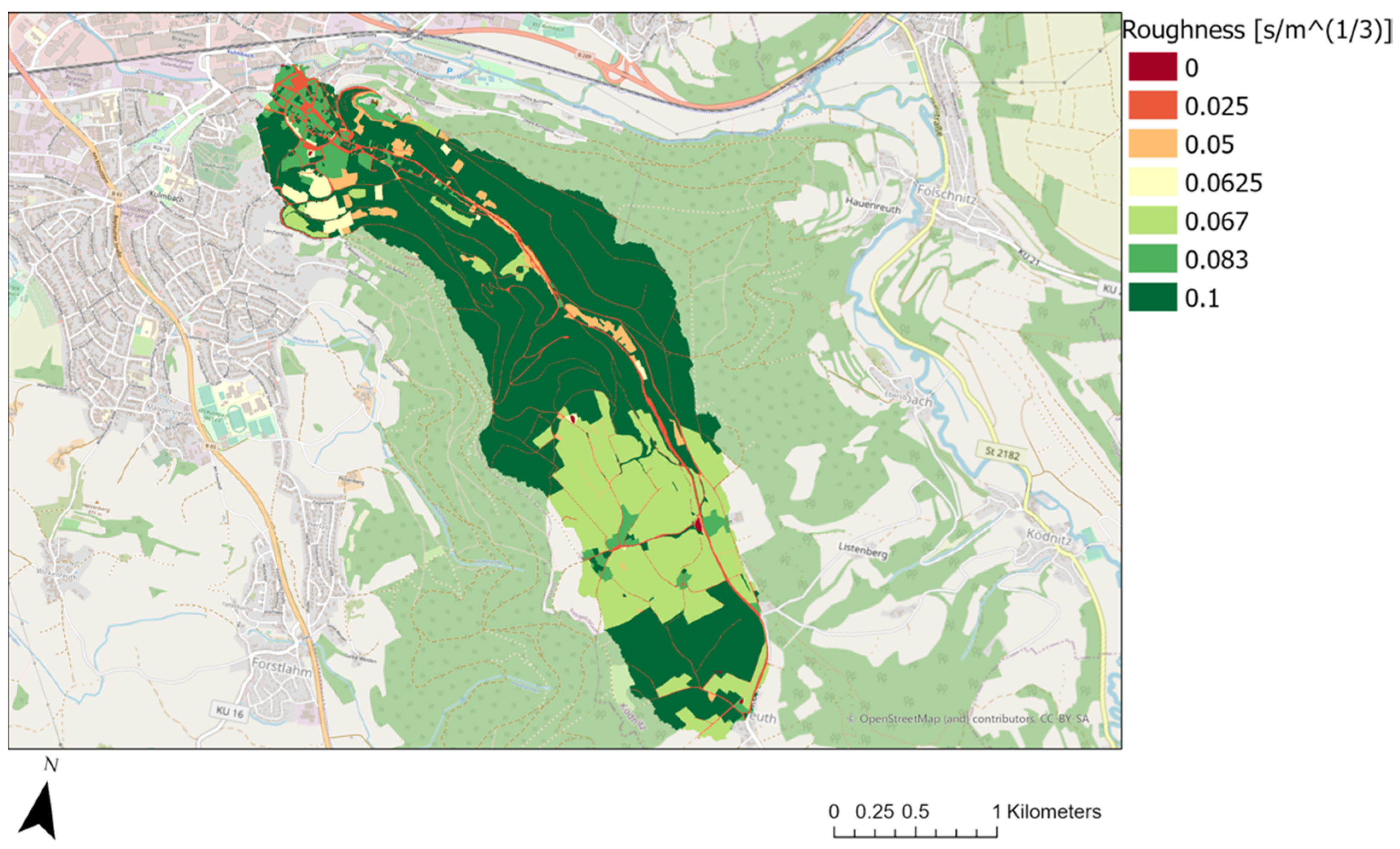
In the first step, the setup of the 1D flow paths is conducted in PCSWMM [24,25]. An automatic delineation function is used to determine the flow path on the 2 m mesh to create an overland drainage network consisting of nodes and VSL. In the second step, the generated drainage system is reduced to sites where the coarser representation of buildings leads to an obstruction of the flow path determined by the 2 m model. In the third step, the generated nodes are converted into storage nodes and outfall nodes, representing the starting point and endpoint of the obstruction. In the fourth and final step, manual adaptions of the flow paths are required for some sites, which in the first run still show an incorrect inundation. Herein, the calculated flow paths of the benchmark model serve as validation for the generated overland drainage network. The shape of the VSL is defined as open rectangular with dimensions according to the represented topography of the considered site. To investigate the influence of the storage volume and to examine if this volume can be used to counteract changes in the building’s contour and steepness of the topography due to the resampling, different storage coefficients of 1, 0.1, and 0 (=no storage) are used. By means of these values, a range of small fractions regarding the cell’s size is considered as storage area. The roughness of VSL is set according to the roughness of the local topography. Thereby, the center of each cell/link decides the value of roughness taken. The pre-processed DEMs and the roughness rasters are used to set up the model for the 2D overland flow model. Rainfall is assigned to the 2D overland flow model. An overview of the isotropic roughness distribution over the case study is shown in Figure 1.
2.2. Model Runs and Validation Strategy
The investigations of the developed VSL are examined for different model resolutions including a 2 m, 5 m, and 10 m mesh resolution. To validate the methodology the results of the 2 m mesh functions are used as a benchmark for the validation procedure since the aim is to improve the results of the models using a coarser grid. The validation is conducted in a two-stage procedure. In the first stage, only a very small area is considered. This is used for verifying the suitability of the method in retaining the flow features of the finer grid. At this stage rainfall intensities of 5, 30 and 50 years return period, namely, 31.6 mm/h, 47.5 mm/h, and 52 mm/h, as well as a rainfall intensity of 40 mm/h are considered. In the second stage, a larger area is used for discussing the method applicability to real cases in terms of accuracy and computational time, and final validation. At this stage, VSL are extended to the whole case study, which consists of an urban dense area in the northwest of the city of Kulmbach (see Section 2.3).
Results are validated by investigating the simulated maximum water depth of all mesh resolutions. The 2 m model is used as observation data and the benchmark model. To deal with the different mesh resolutions, the results of coarser models with a 5 m and 10 m resolution are resampled by a simple nearest neighbor approach to a 2 m resolution with the same extent and cell number. The nearest neighbor approach guarantees that the water depth of each cell is maintained without any averaging and interpolation.
To validate the simulation results, three different goodness-of-fit (GOF) criteria are applied that determine the accordance of the coarser models with the benchmark model. The first GOF constitutes the coefficient of determination r2, which gives information about the linear correlation between simulated (i.e., 5 m and 10 m) and observed data (2 m), as follows:
where Oi = observed value, Pi = predicted value, = average of observed values, = average of predicted values and n = total amount of data. A value of 1 is interpreted as a full correlation and a value of 0 as no correlation. The second GOF is the LogNSE, which weights small values higher and mitigates extreme values, and is calculated as follows:
The range is from −∞ to 1, where 1 means a perfect match of the observed and predicted values. The last GOF is the root mean square error (RMSE), which gives information about the error distribution, and is calculated as follows:
The range of this GOF reaches from 0 to ∞ with a perfect fit at 0.
For further investigation, the confusion matrix is determined by means of the flood extent. The cells are classified into dry and flooded cells, whereas a threshold regarding the max. water depth of 0.1 m is used to define a cell’s state (Table 1).
The cells are classified into the following four categories:
- True positive (TP) = number of cells that are flooded in the simulation and observation;
- True negative (TN) = number of cells that are not flooded in the simulation and observation;
- False positive (FP) = number of cells that are flooded in the simulation, but dry in the observation;
- False negative (FN) = number of cells that are dry in the simulation, but flooded in the observation.
By means of these cells the percentage of the correct prediction of dry and flooded cells is determined by the following expression (Table 2):
2.3. Site Description
Kulmbach is a city in Germany located at the River Main. As a case study, a small part in the southwest of Kulmbach is considered. As shown in Figure 2, the catchment area is characterized by a steep area in the southeast and an urban dense area in the northwest. Since the new approaches focus on buildings, the highly dense area covered by buildings in the northwest is of high interest (red marked area in Figure 2). The case study is chosen due to its steep characteristic, which enhances the blockage effect of buildings.
2.4. Model Description
Hydraulic models are commonly used for flood simulation in urban areas. Depending on the complexity of topography and computational resources, 1D or 2D approximations of the shallow water equations (SWE) are used to simulate the motion of water [26]. These models can simulate the flow routing on complex topographies and thus constitute a common tool for urban flood modeling. In this work, the commercial software Personal Computer Storm Water Management Model (PCSWMM), the 1D Storm Water Management Model (SWMM), and the 2D diffusive wave model P-DWave 2D are used. The mathematical background is given in the following sub-sections.
2.4.1. PCSWMM/SWMM—1D Dynamic Model
PCSWMM is commercial software, which combines the SWMM engine with the support of a geoinformation system for water management tasks. The water transportation is calculated by means of a drainage system consisting of storage nodes, conduits, and outfall nodes. The one-dimensional flow is simulated with the following St. Venant equations:
where Q = discharge [m3/s], t = time [s], A = cross-sectional area [m2], 2, x = distance [m], H = hydraulic head [m], Sf = friction slope (head loss per unit length), S = VSL sink/source term, and g = gravitational constant [m2/s]. The equation for the dynamic routing process is obtained by combining Equations (4) and (5), as follows:
where U = flow velocity [m/s]. By means of finite difference approximations, Equation (6) can be written as follows:
where η = n/1.486. = average cross-sectional area, = average flow velocity [m/s], = average hydraulic radius of the flow cross-section (m). Average values for A, U, and R can be approximated using the heads H1 = hydraulic head at the upstream end of the conduit and H2 = hydraulic head at the downstream end of the conduit (m). It should be noted that there are many established softwares that solve the dynamic equations in a non-conservative form (e.g., HYSTEM-EXTRAN [27], PCSWMM [28], INFOWORKS [29] or MOUSE [30]). This solution has supported the extensive use of such models for practical purposes and experimental validation [31,32,33,34]. SWMM provides two types of nodes, junction nodes without a storage volume or surface area and storage nodes, which contain both properties. The water head H at a certain time step is calculated by the following:
where ASN = storage surface area, ASL = surface area contributed by a connecting link and = net discharge in the node assembly [m3/s]. The geometric shape of a storage unit is defined by a storage coefficient A, an exponent B, and a constant C in the following:
where area = surface area of a storage unit and depth = surface depth above the bottom of a storage unit. A finite difference approximation substitutes the spatial and temporal derivations. In case of a surcharge, the overland flow rate is determined by the following:
where t = current time [s] and ∆t = timestep [s]. Further details can be found in [24].
2.4.2. P-DWave 2D—2D Diffusive Wave Model
P-DWave 2D is a parallelized diffusive wave model [35]. The momentum equation of the 2D SWE is simplified by neglecting all the momentum equations except the pressure and friction term resulting in the following equations:
where g = acceleration due to gravity, z = bed elevation, h = water depth, u = depth average flow velocity vector, S = VSL sink/source term and Sf = bed friction vector [Sfx Sfy]T. The bed friction term is approximated by Manning’s formula The continuity equation is solved by an explicit finite volume method of the first order, whereas a cell-centered control volume discretizes the spatial domain, as follows:
With the following:
where Ai = cell area [m2], i = index of current cell, j = index of adjacent cell, ij = index considering cell i and j, Lij = contact face between cells, uij = water velocity [m/s], hij = water depth [m], In,ij water level surface gradient vector multiplied by unit normal vector, S = sink/source term, n = Manning’s coefficient, t = current time [s] and ∆t = timestep [s]. A prediction-correction wet–dry scheme is applied to obtain absolute mass conservation. Further details can be found in [35].
2.4.3. Coupling Process between SWMM and P-DWave 2D
SWMM 5.1 uses a dynamic link library (DLL) consisting of functions that simplify the linking procedure to other models. The coupling is conducted by adding three additional functions to SWMM 5.1 code called SWMM-Link, SWMM-to-2D, and 2D-to-SWMM. The SWMM-Link DLL enables the extraction of the node ID, crest, and elevation from SWMM, whereas the ID is linked as input data. Furthermore, the function extracts the simulation time and time step of SWMM to initiate and synchronize the linking time step between the two models. The second function SWMM-to-2D uses the node ID as input to exchange the information about the discharge for each simulation time step and extract the node water levels. The last function 2D-to-SWMM exchanges the information about the discharge. The values are positive in case of a water transfer from P-DWave to SWMM or negative otherwise. Herein we assume that the discharge along the VSL can be approximated by a weir equation (Equation (16)) or a submerged weir equation (in case of backwater in the link) (Equation (17)), as follows:
where Q = discharge [m3/s], cw = weir discharge coefficient [-], w = crest width [m], Amh = channel flow area [m2], co = orifice discharge coefficient, Z2D = ground surface elevation in the 2D model, h1D = hydraulic head in the 1D model, h2D = hydraulic head in the 2D model. Equation (16) is applied if h1D < Z2D and Equation (17) if h1D > Z2D. The negative form of the submerged weir equation is applied to calculate the discharge in case of reverse flow, as follows:
Since the time steps of both models differ, the time step of both models needs to be synchronized. Further details can be found in [36].
3. Results
3.1. DSWMM/2DP-DWave 2D Dual-Drainage Model
3.1.1. First Stage of Validation: Test Case
For the first stage, only the test case is considered. The VSL are automatically placed according to the determined flow path in the 2 m model at the location, where the water accumulates incorrectly. This is conducted following the procedure in Section 2.4.1. After the main flow paths are identified in the 2 m model, only the ones crossing between buildings are kept and added to the models with coarser grids in the dual-drainage version. Figure 3 shows an example of the placement of VSL. Figure 4a shows the maximum water depth obtained by the 2 m resolution model. Figure 4b shows the overestimation of the maximum water depth by the 5 m resolution model, if no placement of virtual channels is considered. Figure 4c shows the local improvement obtained with the automatized placement of virtual channels. Figure 4d shows the further local improvement after manual refinement.
For a better interpretation of the results, the test case is additionally divided into several subzones, which are not affected by backwater effects and, hence, are regarded as independent of each other (Figure 3).
The boundaries are chosen to depict the effect on water accumulation and flow development in the vicinity of a building. Therefore, the chosen area covers a small part of the upstream and downstream areas close to buildings, which are highly affected by VSL. Thereby, the 5 m model is subdivided into five subzones and the 10 m model into four subzones.
The procedure in Figure 4 is repeated for each subzone. Each subzone functions as an individual validation area. The calculated GOFs for these areas are shown below (Figure 5).
The GOFs illustrate a general improvement for most of the subzones. The greatest change can be observed in the RMSE for the 10 m model, but the LogNSE also shows a significant increase. The r2 only shows small improvements and has an almost constant trend. The change in the GOFs differs depending on the subzones, and reveals a dependency on individual characteristics of the considered area and the model resolution.
To interpret the effectiveness of the approach, the results are compared to the GOFs obtained by different model resolutions, so the improvements can be better evaluated (Figure 6). The mesh resolutions range from 3 m to 10 m, thus the results of the dual-drainage model can be compared to a wide range. Thereby, the calculated GOFs only refer to the area of the set subzones and do not consider the whole area. Thus, the impact on the flow around buildings can be better evaluated.
The comparison shows an improvement for all the GOFs. The 5 m coupled model approximates the 4 m model for the logNSE and r2. The 10 m model for these GOFs shows larger improvements and approximates the 7 m model for the logNSE, and has a slightly better value than the 7 m model for the r2. The largest improvements can be observed for the RMSE. The 5 m model has a smaller RMSE than the 3 m model, and the 10 m model shows similar values to the 4 m model. Figure 7 shows the confusion matrix for the first stage.
The matrix shows a modest total improvement of 0.9% regarding the 5 m model and 2% when considering the 10 m model with VSL. The TPR of the 5 m model shows a deterioration, observed by the decrease in the percentage of correct predicted flooded cells. To investigate the effectiveness, depending on the rainfall intensity, the difference in total accuracy is determined between the coupled and original model for several rainfall events (Figure 8).
The first three subzones reveal a positive trend, whereas the trend for the fourth and fifth subzones differs. The graphic representation demonstrates an improvement in the total accuracy for values greater than zero. Comparing the results, a difference between the subzones and rainfall intensities can be observed. Apart from the small deterioration in the second subzone (10 m/40 mm) and the fourth subzone (5 m/h N 5, 40 mm, hN 30), the coupling process reveals an improvement of the simulation results. A variation in the defined storage volume by different storage coefficients, and the usage of average width, defined by the minimum and maximum width in the 2 m model, shows no significant improvements in the results.
After the third step of the VSL methodology, the fourth and final step is executed. Herein, manual adaptions are made for sites that still have incorrect flood inundation extents. This step is only conducted for the first (5 m) and fourth subzones (5 m and 10 m), which still reveal larger inundations compared to the benchmark model, due to the different arrangement and size of the buildings. The flow path of the benchmark model is used as a template to adapt the flood routing, according to the more precise flow in the 2 m model. The determined GOFs after the fourth step are shown in Figure 9.
By means of the additional manual adaption, the accordance with the benchmark model can be significantly enhanced. The deterioration for the 10 m model in the fourth subzone also reveals that this should be conducted with caution. The usage of different storage coefficients shows no significant changes.
The error in the maximum water volume, only considering the subzones, is significantly reduced. The deviation, with regards to the benchmark model, for the 5 m model is reduced from 69.63% to 29.73%, only considering step 1–3, and to 5.03% when the manual adaption in step 4 of the VSL methodology is included. Regarding the 10 m model, the deviation is reduced from 152.75% to 22.92%, and to 19.16%, considering the fourth step of the VSL methodology.
3.1.2. Second Stage of Validation: Case Study
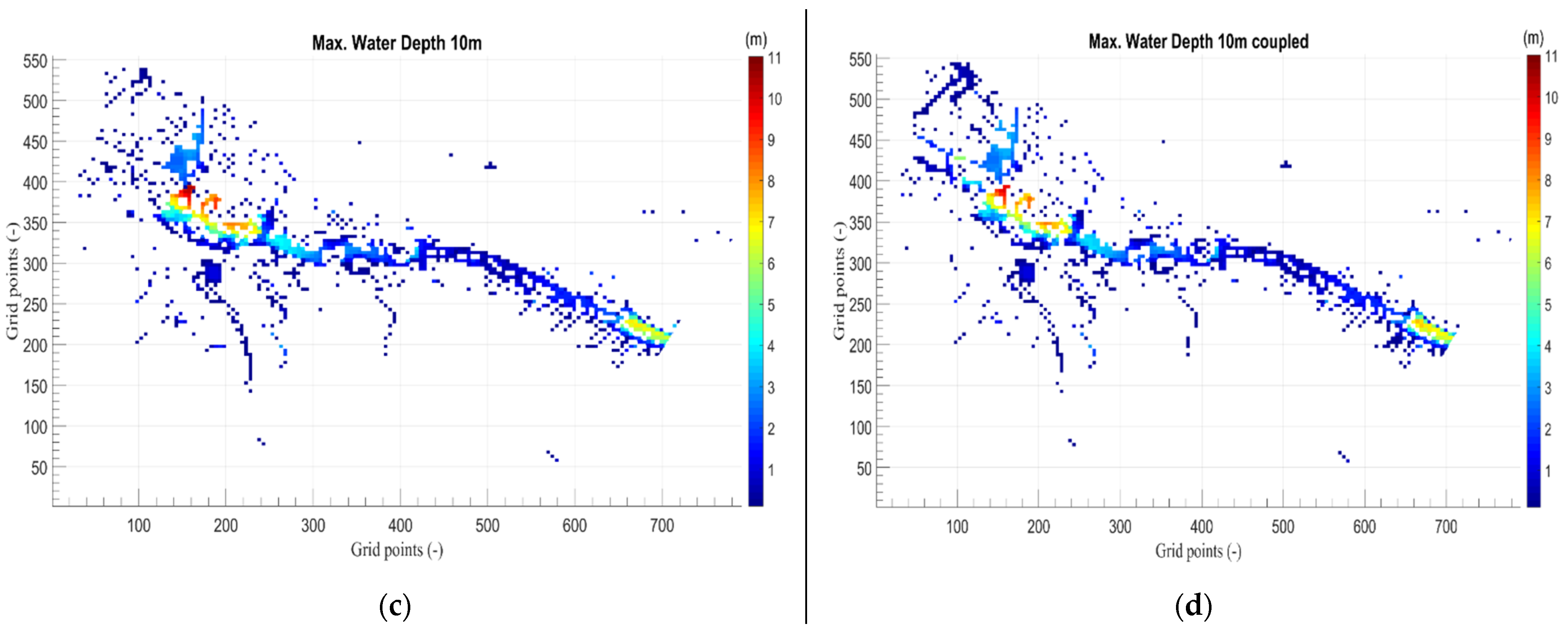
Given the overall improvement in the first stage, the procedure is now applied to the whole case study area. The results of the inundation are shown in Figure 10.
The implementation of VSL by coupling leads to contrary effects on the inundation in the 5 m and 10 m models. The greatest effect can be observed around the grid points (200, 350). The 5 m model shows an increase in inundation depth for this area, whereas the coupling in the 10 m model leads to a decrease. The results indicate a generally higher consistent flow, which is also shown by the higher water depths in the 10 m model at the catchment’s outlet at the grid points around (100, 500). The calculated GOFs are shown in Figure 11.
The GOFs demonstrate that the usage of VSL enhances the simulation results. Only the RMSE for the 5 m model deteriorates slightly. Since a larger area is considered, as for the test case/subzones, the improvements are less significant. Since the dense area complicates the manual adaptation after the first coupling process, this procedure is primarily conducted in the rural area around the dense urban area. Consequently, the additional modifications do not result in large changes in the GOFs. The deterioration in the 10 m model, for the RMSE, reveals that the adaptions can also have negative impacts on the flow.
The confusion matrix in Figure 12 additionally demonstrates a total improvement of the predicted dry and flooded cells. The total accuracy rises by 0.1% for the 5 m model and 0.7% for the 10 m model. The TNR and TPR also show a better prediction of dry cells for the urban area in the 5 m model, but a worse prediction of flooded cells and an improvement for both states in the 10 m model.
The biggest advantage of resampling constitutes the faster computation time. By using a 5 m grid instead of a 2 m resolution, the computation time can be reduced by 92.6%, and by 99% when using a 10 m grid. The implementation of VSL slows down the runtime minimally, due to the coupling process, with a reduction of 91.2% for the 5 m model and 98.5% for the 10 m model, compared to the benchmark model.
Considering the change in maximum water volume, the volume of water increases in the area of interest. Thus, the deviation with regard to the benchmark model rises slightly, from 6.28% to 7.96%, for the 5 m model, and from 28.64% to 29.66% for the 10 m model. However, considering the whole catchment area, an improvement in the deviation, from 5.27% to 4.57%, for the 5 m model, and from 24.46% to 23.86% for the 10 m model, is still achieved, highlighting the benefit of the developed approach.
4. Discussion
By means of the VSL approach, the flood routing in coarse grids is adapted to the flow paths in the fine mesh in the case of incorrect water accumulation. These occur primarily due to missing flow paths between buildings, overestimation of the building’s size, or differences in contour and form. Hence, incorrect inundations are reduced, allowing a more continuous flow.
The GOFs (Figure 5) show that the simulation results can be significantly enhanced by implementing VSL in a 1D/2D model. Incorrect water accumulations can thus be reduced and the flow path can be adjusted according to a finer model resolution. The approach shows higher effectiveness for the 10 m model, indicating a better performance the coarser the grid is. The differences in the improvement of the GOFs, depending on the subzones, are traced back to the individual characteristics of each area. Thereby, especially the number and size of the buildings represent an important factor, but also the topography (i.e., depressions, steepness, etc.). Depending on the rainfall, the improvements can differ. Thereby, no clear trend with a higher rainfall intensity can be observed. This stems from the variation in flow routing based on the rainfall. For example, for very large rainfall intensity, depressions in the topography can be overcome, resulting in more inundation areas and affecting the flow direction. Moreover, backwater effects can change, leading to higher inundation in the upstream direction. Consequently, the effectiveness of the VSL approach can vary depending on the flow regime for a given rainfall event.
The comparison with other model resolutions shows a negative trend the coarser the grid is (Figure 6). Nevertheless, deviations from this trend, for a highly coarse grid (i.e., 8–10 m), can be observed. These deviations are limited to the coarsest grids, where the GOF’s value and their differences are small, due to general low agreement with the benchmark model. Thus, an already small variation in the building’s representation can lead to positive and negative influences on the overall agreement.
The additional modifications and adaptions of the flow path in the fourth step of the VSL methodology focus on water depth reductions, which are not clearly identifiable during the first coupling process (Figure 9). The adaptions can have significant positive impacts on the simulation. Since this process risks transporting too much water downwards, this should be conducted with caution, to avoid deterioration in the simulation results. Moreover, highly urban dense areas, with large inundations, complicate the procedure, since significant locations, which are responsible for an incorrect accumulation, become difficult to identify.
The determination of flood extent and confusion matrix demonstrates that the VSL approach also risks having a negative impact on the prediction of flooded cells (Figure 7). This is the result of flooding being underpredicted in the upstream direction of the buildings, due to an overprediction of the water amount, which is conveyed downwards. This is promoted by the contours of the buildings, which are smoothed by the resampling procedure. Thus, areas where water accumulates due to the complex contours of a building are reduced (or disappear) in coarser grids. By placing VSL at a coarse cell, a larger area is directly affected. The coarser the grid is, the higher the error of the accumulation due to the complex building’s contour becomes. The larger water amount conveyed by VSL can also lead to an overestimation of flooding in the downstream direction. To avoid both phenomena, the flow through VSL may require a post-calibration for limiting the discharges. For post-calibration, the authors would suggest the use of the storage parameters in Equation (9), which determine the surface area of a storage unit, as the calibration parameter, and the observed error in flooded volume as the objective function. The determination of the maximum flooded volume around the buildings is particularly effective for areas with a low density, and where incorrect inundations result primarily from an overestimated size of the buildings.
The application on a highly dense area illustrates that the VSL approach can have two opposite effects (Figure 10). On the one hand, the water depth can increase, since water in the upstream direction is allowed to flow downwards, but accumulates downstream due to the resampling effects, such as larger depressions in topography and different flow paths (as compared to high-resolution grids). On the other hand, the maximum water depth is reduced upstream, due to a more continuous flow, allowing the water to be drained. Therefore, the implementation of VSL can also lead to a slight overestimation of flooding in localized areas. Nevertheless, the confusion matrix clearly demonstrates an improvement in the simulation of the flood extent and distribution obtained by the proposed approach (Figure 11 and Figure 12). Compared to the test case, the improvements in the larger urban dense area are less obvious because of the more complex dynamics of the flood routing.
Another advantage of the proposed VSL methodology is that if the flow regime becomes critical around buildings and through narrow gaps, the 1D model, based on the dynamic flow equations, would still be able to solve it. This is an advantage, since some 2D urban flood models (such as the model tested in this study) do neglect the inertia terms in the shallow water equations and cannot capture these localized phenomena. In any case, it should be stated that applying the full dynamic model per se does not guaranty that such features will be captured. In fact, if the resolution is not fine enough (e.g., 0.1 m for the typical benchmark hydraulic jump over an obstacle [37]), both the diffusive wave and full dynamic model would produce similar solutions. This supports the fact that in many urban flood studies, the diffusive wave often performed equally well [21,38], or even out-performed other shallow water models where real data were available [39].
5. Conclusions
The resolution at which buildings are represented in 2D models affects the quality of the numerical simulation of floods in urban areas. Accumulation around buildings increases, due to the coarser and larger representation of buildings and the missing flow paths between them. The degree to which the water depths differ from finer resolutions depends primarily on the size, density, and arrangement of the buildings.
These adverse effects of resampling can be significantly reduced by implementing the proposed VSL, by including the flow path in coarser models, based on a fine resolution model. The method enables narrow flow paths between buildings to be considered, and allows water to flow through buildings, which incorrectly leads to inundation in coarser grids. Overall improvements in a larger area can be smaller or bigger depending on the local impact of the missing flow paths. In any case, it was shown that incorrect accumulations around buildings could be significantly reduced. The reduction in the max. water volume, from 69.63% to 5.03%, using a 5 m grid, and from 152.75% to 22.92% for a 10 m grid demonstrates a significant improvement for smaller areas with a lower density of buildings. The VSL methodology is thus more appropriate for areas in which flow paths are well defined.
Further research needs to be conducted on the possibility of underestimating flooding in the upstream direction and overestimation in the downstream direction of a building, if too much water is conveyed downstream. Even if dry cells are better predicted, the approach can lead, in some cases, to a deterioration in the simulation of flooded cells. To reduce this effect, a calibration procedure was investigated. It was shown that a manual procedure can significantly improve the results. However, the suggested procedure becomes more complex for highly dense areas, making it a non-trivial optimization problem. Given the significant improvement, in terms of run times gained by the VSL, the future focus could be on its application to flood forecast systems.
Author Contributions
Conceptualization, S.R. and J.L.; methodology, S.R. and J.L.; software, S.R. and J.L.; validation, S.R.; formal analysis, S.R.; investigation, S.R.; resources, J.L. and Q.L. data curation, S.R.; writing—original draft preparation, S.R.; writing—review and editing, all authors; visualization, S.R.; supervision, J.L. and Q.L.; project administration, S.R. and J.L. All authors have read and agreed to the published version of the manuscript.
Funding
This research was funded by Bavarian State Ministry of the Environment and Consumer Protection (StMUV) with the grant number 69-0270-50433/2017. The APC was funded by Technical University of Munich.
Acknowledgments
The research presented in this paper has been carried out as part of the HiOS project (Hinweiskarte Oberflächenabfluss und Sturzflut) funded by the Bavarian State Ministry of the Environment and Consumer Protection (StMUV) and supervised by the Bavarian Environment Agency (LfU).
Conflicts of Interest
The authors declare that they have no known competing financial interest or personal relationships that could have appeared to influence the work reported in this paper.
References
- Şen, Z. Flood Modeling, Prediction and Mitigation; Springer: Cham, Switzerland, 2018. [Google Scholar]
- Sene, K. Flash Floods; Springer: Dordrecht, The Netherlands, 2013. [Google Scholar]
- Sampson, C.C.; Fewtrell, T.J.; Duncan, A.; Shaad, K.; Horritt, M.S.; Bates, P.D. Use of terrestrial laser scanning data to drive decimetric resolution urban inundation models. Adv. Water Resour. 2012, 41, 1–17. [Google Scholar] [CrossRef]
- Gallegos, H.A.; Schubert, J.E.; Sanders, B.F. Two-dimensional, high-resolution modeling of urban dam-break flooding: A case study of Baldwin Hills, California. Adv. Water Resour. 2009, 32, 1323–1335. [Google Scholar] [CrossRef]
- Paquier, A.; Mignot, E.; Bazin, P.-H. From Hydraulic Modelling to Urban Flood Risk. Procedia Eng. 2015, 115, 37–44. [Google Scholar] [CrossRef]
- Betsholtz, A.; Nordlöf, B. Potentials and Limitations of 1D, 2D and Coupled 1D-2D Flood Modelling in HEC-RAS. Master’s Thesis, University Lund, Lund, Sweden, 2017. [Google Scholar]
- de Almeida, G.A.M.; Bates, P.; Ozdemir, H. Modelling urban floods at submetre resolution: Challenges or opportunities for flood risk management? J. Flood Risk Manag. 2018, 11, S855–S865. [Google Scholar] [CrossRef] [Green Version]
- Esri Resampling. Available online: https://desktop.arcgis.com/de/arcmap/10.3/tools/data-management-toolbox/resample.htm (accessed on 9 May 2021).
- Vojinovic, Z.; Seyoum, S.; Salum, M.H.; Price, R.K.; Fikri, A.K.; Abebe, Y. Modelling floods in urban areas and representation of buildings with a method based on adjusted conveyance and storage characteristics. J. Hydroinform. 2012, 15, 1150–1168. [Google Scholar] [CrossRef]
- Fewtrell, T.; Bates, P.; Horritt, M.; Hunter, N. Evaluating the effect of scale in flood inundation modelling in urban environments. Hydrol. Process. 2008, 22, 5107–5118. [Google Scholar] [CrossRef]
- Chen, A.; Evans, B.; Djordjević, S.; Savic, D. A coarse-grid approach to representing building blockage effects in 2D urban flood modelling. J. Hydrol. 2012, 426, 1–16. [Google Scholar] [CrossRef] [Green Version]
- Yu, D.; Lane, S.N. Urban fluvial flood modelling using a two-dimensional diffusion-wave treatment, part 1: Mesh resolution effects. Hydrol. Process. 2006, 20, 1541–1565. [Google Scholar] [CrossRef]
- Maksimovic, C.; Prodanovic, D. Modelling of Urban Flooding—Breakthrough or Recycling of Outdated Concepts. In Urban Drainage Modeling; American Society of Civil Engineers: Reston, VA, USA, 2001; pp. 1–9. [Google Scholar]
- Mark, O.; Weesakul, S.; Apirumanekul, C.; Aroonnet, S.B.; Djordjević, S. Potential and limitations of 1D modelling of urban flooding. J. Hydrol. 2004, 299, 284–299. [Google Scholar] [CrossRef]
- Neal, J.; Fewtrell, T.; Bates, P.; Wright, N. A comparison of three parallelisation methods for 2D flood inundation models. Environ. Model. Softw. 2010, 25, 398–411. [Google Scholar] [CrossRef]
- Guo, K.; Guan, M.; Yu, D. Urban surface water flood modelling—A comprehensive review of current models and future challenges. Hydrol. Earth Syst. Sci. 2021, 25, 2843–2860. [Google Scholar] [CrossRef]
- MacNeice, P.; Olson, K.M.; Mobarry, C.; de Fainchtein, R.; Packer, C. Paramesh: A parallel adaptive mesh refinement community toolkit. Comput. Phys. Commun. 2000, 126, 330–354. [Google Scholar] [CrossRef] [Green Version]
- Chang, C.-H.; Chung, M.-K.; Yang, S.-Y.; Hsu, C.-T.; Wu, S.-J. Improving the Computational Performance of an Operational Two-Dimensional Real-Time Flooding Forecasting System by Active-Cell and Multi-Grid Methods in Taichung City, Taiwan. Water 2018, 10, 319. [Google Scholar] [CrossRef] [Green Version]
- Sanders, B.F.; Schubert, J.E. PRIMo: Parallel raster inundation model. Adv. Water Resour. 2019, 126, 79–95. [Google Scholar] [CrossRef]
- Dewals, B.; Bruwier, M.; Pirotton, M.; Erpicum, S.; Archambeau, P. Porosity Models for Large-Scale Urban Flood Modelling: A Review. Water 2021, 13, 960. [Google Scholar] [CrossRef]
- Leandro, J.; Schumann, A.; Pfister, A. A step towards considering the spatial heterogeneity of urban key features in urban hydrology flood modelling. J. Hydrol. 2016, 535. [Google Scholar] [CrossRef]
- Schubert, J.E.; Sanders, B.F. Building treatments for urban flood inundation models and implications for predictive skill and modeling efficiency. Adv. Water Resour. 2012, 41, 49–64. [Google Scholar] [CrossRef]
- Chen, A.; Djordjević, S.; Leandro, J.; Savic, D. The urban inundation model with bidirectional flow interaction between 2D overland surface and 1D sewer networks. In Proceedings of the NOVATECH 2007, Lyon, France, 25 June 2007; pp. 465–472. [Google Scholar]
- Rossman, L.A. Storm Water Management Model Reference Manual Volume II—Hydraulics; U.S. Environmental Protection Agency: Washington, DC, USA, 2017.
- Rossman, L.A.; Huber, W.C. Storm Water Management Model Reference Manual Volume I—Hydrology (Revised); U.S. Environmental Protection Agency: Washington, DC, USA, 2016.
- Crispino, G.; Gisonni, C.; Iervolino, M. Flood hazard assessment: Comparison of 1D and 2D hydraulic models. Int. J. River Basin Manag. 2015, 13, 153–166. [Google Scholar] [CrossRef]
- Itwh HYSTEM-EXTRAN. Available online: https://itwh.de/en/software-products/desktop/hystem-extran/ (accessed on 18 September 2021).
- CHI PCSWMM. Available online: https://www.pcswmm.com/ (accessed on 18 September 2021).
- Innovyze Basic 2D Hydraulic Theory. Available online: https://help2.innovyze.com/infoworksicm/Content/HTML/ICM_ILCM/Basic_2D_Hydraulic_Theory.htm (accessed on 16 September 2021).
- DHI. MOUSE Pipe Flow Reference Manual; DHI: New York, NY, USA, 2019. [Google Scholar]
- Freni, G.; Ferreri, G.; Tomaselli, P. Ability of Software SWMM to Simulate transient sewer smooth pressurization. Water Sci. Technol. J. Int. Assoc. Water Pollut. Res. 2010, 62, 1848–1858. [Google Scholar]
- Kourtis, I.; Kopsiaftis, G.; Bellos, V.; Tsihrintzis, V. Calibration and validation of SWMM model in two urban catchments in Athens, Greece. In Proceedings of the International Conference on Environmental Science and Technology (CEST), Rhodes, Greece, 31 August–2 September 2017. [Google Scholar]
- Vasconcelos, J.; Eldayih, Y.; Zhao, Y.; Jamily, J. Evaluating Storm Water Management Model Accuracy in Conditions of Mixed Flows. J. Water Manag. Model. 2018, 27, C451. [Google Scholar] [CrossRef] [Green Version]
- Niazi, M.; Nietch, C.; Maghrebi, M.; Jackson, N.; Bennett, B.; Tryby, M.; Massoudieh, A. Storm Water Management Model: Performance Review and Gap Analysis. J. Sustain. Water Built Environ. 2017, 3, 04017002. [Google Scholar] [CrossRef] [PubMed] [Green Version]
- Leandro, J.; Chen, A.S.; Schumann, A. A 2D parallel diffusive wave model for floodplain inundation with variable time step (P-DWave). J. Hydrol. 2014, 517, 250–259. [Google Scholar] [CrossRef]
- Leandro, J.; Martins, R. A methodology for linking 2D overland flow models with the sewer network model SWMM 5.1 based on dynamic link libraries. Water Sci. Technol. J. Int. Assoc. Water Pollut. Res. 2016, 73, 3017–3026. [Google Scholar]
- Hafnaoui, M.; Carvalho, R.; Debabeche, M. Prediction of Hydraulic Jump location in Some Types of Prismatic Channels using Numerical Modelling. In Proceedings of the 6th International Junior Researcher and Engineer Workshop on Hydraulic Structures (IJREWHS 2016), Lübeck, Germany, 30 May–1 June 2016. [Google Scholar]
- Martins, R.; Leandro, J.; Chen, A.; Djordjević, S. A comparison of three dual drainage models: Shallow water vs. local inertial vs. diffusive wave. J. Hydroinform. 2017, 19, jh2017075. [Google Scholar]
- Pflugbeil, T.; Roich, K.; Disse, M. Hydrodynamic simulation of the flash flood events in Baiersdorf and Simbach (Bavaria)—A model comparison. EGU Gen. Assem. 2019, 21, 15509. [Google Scholar]
Figure 1.
Applied Manning roughness coefficients for the case study.

Figure 2.
Catchment area and topography of the study area. (a) Pre-validation area for the first stage of the validation procedure; (b) final validation area for the second stage of the validation procedure.
Figure 2.
Catchment area and topography of the study area. (a) Pre-validation area for the first stage of the validation procedure; (b) final validation area for the second stage of the validation procedure.

Figure 3.
Subdivision into subzones, as follows: (a) subzones for the 5 m model; (b) subzones for the 10 m model.
Figure 3.
Subdivision into subzones, as follows: (a) subzones for the 5 m model; (b) subzones for the 10 m model.


Figure 4.
(a) Simulated max. water depth by the 2 m resolution model; (b) overestimation of the max. water depth by the 5 m resolution model due to incorrect water accumulation; (c) improved simulated max. water depth by the 5 m model with automatized placement of virtual channels; (d) further improvement of the simulated max. water depth by the 5 m model after manual refinement.

Figure 5.
Calculated GOFs for each subzone in the 5 m and 10 m model.

Figure 6.
GOFs for different model resolutions and for the coupled models of 5 m and 10 m.

Figure 7.
Confusion matrix considering the subzones.

Figure 8.
Total accuracy for different rainfall events (hN5 = 31.6 mm/h, hN30 = 47.5 mm/h, hN50 = 52 mm/h).
Figure 8.
Total accuracy for different rainfall events (hN5 = 31.6 mm/h, hN30 = 47.5 mm/h, hN50 = 52 mm/h).

Figure 9.
GOFs for the original (2 m), first coupling and the additional manual adaption (modified).
Figure 9.
GOFs for the original (2 m), first coupling and the additional manual adaption (modified).

Figure 10.
(a) Inundation in the 5 m model before the coupling process; (b) inundation in the 5 m model after the coupling process; (c) inundation in the 10 m model before the coupling process; (d) inundation in the 10 m model after the coupling process.
Figure 10.
(a) Inundation in the 5 m model before the coupling process; (b) inundation in the 5 m model after the coupling process; (c) inundation in the 10 m model before the coupling process; (d) inundation in the 10 m model after the coupling process.


Figure 11.
GOFs for the dense urban area.

Figure 12.
Confusion matrix considering all cells in the urban dense area.


Table 1.
Schematic of confusion matrix.
| Observation (2 m Simulation) | ||||
|---|---|---|---|---|
| Dry (0) | Flooded (1) | |||
| Stimulation | Dry (0) | True negative (0/0) | False negative (0/1) | NPV FOR |
| Flooded (1) | False positive (1/0) | True positive (1/1) | PVV FDR | |
| TNR FPR | TPR FNR | Total Accuracy | ||
Table 2.
Determined terms by means of the confusion matrix.
| Type | Description | Equation |
|---|---|---|
| Positive predictive value (PVV) | Percentage of correctly predicted flooded cells | |
| False discovery rate (FDR) | Percentage of wrongly predicted flooded cells | |
| False omission rate (FOR) | Percentage of wrongly predicted dry cells | |
| Negative predictive value (NPV) | Percentage of correctly predicted dry cells | |
| True positive rate (TPR) | Percentage of flooded cells that are also simulated as flooded | |
| False negative Rate (FNR) | Percentage of flooded cells that are not simulated as flooded | |
| False positive rate (FPR) | Percentage of flooded cells that are not simulated as dry | |
| True negative Rate (TNR) | Percentage of flooded cells that are also simulated as dry | |
| Total accuracy (ACC) | Percentage of the overall correctly simulated cells |
Publisher’s Note: MDPI stays neutral with regard to jurisdictional claims in published maps and institutional affiliations. |
© 2021 by the authors. Licensee MDPI, Basel, Switzerland. This article is an open access article distributed under the terms and conditions of the Creative Commons Attribution (CC BY) license (https://creativecommons.org/licenses/by/4.0/).
Share and Cite
MDPI and ACS Style
Ramsauer, S.; Leandro, J.; Lin, Q. Inclusion of Narrow Flow Paths between Buildings in Coarser Grids for Urban Flood Modeling: Virtual Surface Links. Water 2021, 13, 2629. https://doi.org/10.3390/w13192629
AMA Style
Ramsauer S, Leandro J, Lin Q. Inclusion of Narrow Flow Paths between Buildings in Coarser Grids for Urban Flood Modeling: Virtual Surface Links. Water. 2021; 13(19):2629. https://doi.org/10.3390/w13192629
Chicago/Turabian StyleRamsauer, Sebastian, Jorge Leandro, and Qing Lin. 2021. "Inclusion of Narrow Flow Paths between Buildings in Coarser Grids for Urban Flood Modeling: Virtual Surface Links" Water 13, no. 19: 2629. https://doi.org/10.3390/w13192629
Note that from the first issue of 2016, this journal uses article numbers instead of page numbers. See further details here.