Article

Interpreting the Manning Roughness Coefficient in Overland Flow Simulations with Coupled Hydrological-Hydraulic Distributed Models

by
Marcos Sanz-Ramos
1,*,
Ernest Bladé
1,
Fabián González-Escalona
2,
Gonzalo Olivares
1 and
José Luis Aragón-Hernández
2
1
Flumen Institute, Universitat Politècnica de Catalunya (UPC)-International Centre of Numerical Methods in Engineering (CIMNE), 08034 Barcelona, Spain
2
División de Ingenierías Civil y Geomática, Facultad de Ingeniería, Universidad Nacional de México (UNAM), Ciudad de México 04510, Mexico
*
Author to whom correspondence should be addressed.
Water 2021, 13(23), 3433; https://doi.org/10.3390/w13233433
Submission received: 12 November 2021 / Revised: 29 November 2021 / Accepted: 1 December 2021 / Published: 3 December 2021

Abstract

:
There is still little experience on the effect of the Manning roughness coefficient in coupled hydrological-hydraulic distributed models based on the solution of the Shallow Water Equations (SWE), where the Manning coefficient affects not only channel flow on the basin hydrographic network but also rainfall-runoff processes on the hillslopes. In this kind of model, roughness takes the role of the concentration time in classic conceptual or aggregated modelling methods, as is the case of the unit hydrograph method. Three different approaches were used to adjust the Manning roughness coefficient in order to fit the results with other methodologies or field observations—by comparing the resulting time of concentration with classic formulas, by comparing the runoff hydrographs obtained with aggregated models, and by comparing the runoff water volumes with observations. A wide dispersion of the roughness coefficients was observed to be generally much higher than the common values used in open channel flow hydraulics.

1. Introduction

The estimation of overland flow is one of the most relevant processes when assessing the hydrological response of a basin. Despite hydrological processes being extremely complex and, nowadays, still not fully understood, their evaluation is essential to characterize the basin flow production under rainfall events. The characterisation of overland flow is a crucial aspect for flood hazard management, which is the most catastrophic natural hazard and results in the greatest material and life damages all over the world [1,2,3]. The flow characteristics are key inputs to perform particular risk analyses as well as for integrating into flood risk early warning systems [4,5,6,7].
Numerical modelling is a widely extended technique that allows studying this kind of complex phenomena for which, in general, no analytical solutions exist. Hydrological modelling has been traditionally performed by means of the so-called aggregated models [7,8], which rely on the simplification of the study area as a single whole unit (generally the basin) or as the contribution (or “aggregation”) of different parts (subbasins) constituting it all linked through a routing method. These models are usually based on conceptual or empirical formulations to describe several physical processes related to precipitation, infiltration, vegetation interception, overland storage, surface runoff, etc., and normally use a representation of the basin, or subbasins, as a homogenous unit [9].
In this aggregated approach, one of the fundamental parameters needed for the transformation of the rainfall into runoff is the time of concentration ( t c ). At present, the concept is still affected by significant ambiguities and uncertainties [10,11] due to the long history of different, and sometimes contradictory, definitions, formulations, and application methodologies. Recently, Beven [12] conducted an exhaustive study on the history of this parameter, questioning at some point the convenience of referring to it as “time of concentration’’ and suggesting that in most cases "time of equilibrium” would be more precise. Although the time of concentration term seems to date back to 1851 [13], Beven points out the discrepancies between two common classes of definitions. On the one hand, there are definitions like the one by the International Glossary of Hydrology [14] that defines t c as “the period of time required for storm runoff to flow from the most remote part of a drainage basin to the outlet”; on the other hand, there are those referred to computational definitions, such as the one by the NCRS [15] that is “the time from the end of excess rainfall to the point of inflection on the receding limb of the hydrograph”. The first family of definitions associate t c to the water velocity, while the second one to the propagation or the flood wave celerity. The second definition is related to the use of the SCS-Unit Hydrograph method [16], one of the most-extended methods for aggregate modelling, which is the basis for many empirical formulas to estimate the value of t c . The difference on the mathematical expression of the different formulas might be due to the parameter dependence on the physiographic characteristics of the basin, some of which may be relevant in some specific basins but not necessarily in others [10,11], but also to the conceptual approach. The use of one or the other approach is related to scientific or technological tradition. For example, in Spain, the formula proposed by Témez [17] is the one used most commonly for estimating t c , which in this case is defined as “the time from the end of rainfall excess to the end of the direct runoff”, while in Mexico there is a long tradition of using the Kirpich formula [18], which was derived empirically by adjusting computations to observed hydrographs, and is commonly used together with the SCS-UH method. According to local authorities and researchers [19,20,21], it is adequate for reproducing the hydrological response of local basins.
The ambiguity in the definition of t c has some important practical consequences, i.e., when estimating the lag time ( t l a g ) parameter to perform a rainfall-runoff computation using the dimensionless SCS-UH method. t l a g is “the time difference between the centre of mass of rainfall excess and the peak of the Unit Hydrograph (UH)” [16]. When using the SCS-UH, t l a g is approximated as 0.6-times t c . If using the t c definition by Témez [17], t l a g should be evaluated as 0.35-times t c [22]. From the previous assertions, it results that the values of t c differs by a factor of around 1.7 times if one or the other definition is used. Obviously, the selection of either formula/definition combination can lead to an overestimation or underestimation of t c , consequently affecting the hydrological processes modelling results and their precision.
More recently, advances in surface hydrology knowledge and developments in numerical modelling techniques, linked to continuous advances on computational performance, led to developments in hydrological modelling tools. Among them, distributed physically-based models are nowadays widely extended [23]. These models have several advantages with respect to aggregated models, such as the ability to account for spatial variability of the rain and physical properties of the basin in their calculations [24]. Within this family of distributed models, there are currently several numerical modelling tools that integrate two-dimensional hydraulic simulations with distributed hydrological modelling [1,25,26,27,28,29,30,31,32]. These integrated or coupled hydrological-hydraulic distributed models use a two-dimensional mesh to discretize the study area. The governing equations are solved on each mesh element by means of a numerical method and scheme, the most common one nowadays probably being the finite volume method [33]. The equations to be solved in each element depend on the local terrain characteristics, such as topography, as well as the parameters, also at each element, that take part in the equations of each of the processes to be simulated. Thanks to this detailed discretisation, and to the fact that hydraulic and hydrological processes are solved jointly at the same time, distributed models achieve more accurate results than the traditional methodology, which consists of first performing a hydrologic simulation with an aggregated model, and subsequently using a hydraulic model to characterize the flow. This coupled model technique usually implies solving the equations of mass and momentum conservation in two dimensions, i.e., the two-dimensional shallow water equations (2D-SWE). In these, the hydrological processes (rainfall-runoff transformation and losses) are usually considered as source terms of the mass conservation equation, and their contribution to momentum is considered only in a few cases.
Both aggregated and coupled hydrological-hydraulic distributed models depend on a large number of parameters (e.g., soil and land characteristics, vegetation, topography, atmospheric conditions, etc.) [34,35,36,37], but also depend on the practitioner’s expertise. Nevertheless, coupled distributed models constitute a conceptual change with respect to aggregated models as they are based on a physical approach. This means that the routing of overland flow is dependent on the terrain roughness and is considered in the model with hydraulic equations, commonly the Manning equation. Thus, the parameters: time of concentration ( t c ) and lag time ( t l a g ) are no longer part of the modelling process, with the Manning roughness coefficient being the only parameter apart from geometry that conditions the runoff propagation.
For hydraulic applications, the Manning roughness coefficient has been widely studied; numerous publications and guidelines for its estimation in natural or artificial channels exist [38,39,40]. However, in coupled hydrological-hydraulic distributed modelling, the value of roughness coefficients must incorporate not only the material roughness itself, but also all the sub-grid geometric features that affect friction, or energy dissipation, and thus the water depth and flow velocity [38]. It is worth mentioning that the flow patterns of overland flow in hydrological models are totally different than for standard uniform steady open channel flow, for which the Manning equation was originally introduced. In hydrological applications, the water depth values can be of a few millimetres or less. Thus, the roughness coefficient values for these extremely shallow overland flows characteristic of hydrological applications can, by no means, be those in the aforementioned guidelines, or at least, those must be questioned and verified. For overland flows, such as those on hillsides, the coefficient values tend to be higher than common ones used in river or stream flows [31,41,42]. Moreover, in coupled hydrological-hydraulic distributed models, the terrain roughness is a fundamental parameter that governs water propagation. It, together with the geometry discretisation, takes the role of determining the basin response as the time of concentration does in aggregated hydrological models.
This work aims to provide insight on the role of the Manning roughness coefficient in overland flow simulations by means of two-dimensional coupled hydrological-hydraulic distributed numerical models, and, thus, to assist in the construction of more accurate distributed rainfall-runoff models. For that purpose, three different strategies were used to characterize the hydrological response of a basin. The first one is a set of four small basins where the concentration time was estimated using empirical formulas and the Manning coefficient in the distributed model was adjusted for the S-shaped hydrograph to fit with the concentration time. In the second case, the resulting hydrograph obtained by means of traditional aggregated hydrological modelling in a basin was used to calibrate the terrain roughness in a 2D-SWE-based distributed model. Finally, the last strategy consisted of the calibration of the roughness coefficients of a monitored basin to adjust the computed results in four observed rainfall events.

2. Materials and Methods

As already introduced in the previous section, two different modelling approaches were used in the present work: (1) traditional aggregated hydrological modelling and (2) coupled hydrologic-hydraulic distributed modelling. The two techniques are briefly presented in the following sections.

2.1. Aggregated Hydrological Modelling

Case Study 2, which consists of a 1016 km2 basin located in Mexico, was firstly analysed with an aggregated hydrological modelling approach through the HEC-HMS software [43]. A standard methodology was applied, based on the local administration guidelines, to discretize the basin. The unit hydrograph (UH) methodology was used for the rainfall-runoff transformation processes, which was obtained from the dimensionless unit hydrograph of the Soil Conservation Service [16,44]. The t l a g parameter and the value of the time of concentration ( t c ) were estimated by means of the Kirpich formula. Precipitation losses were accounted for using the SCS-CN method [44,45], also referred to as the NRCS-CN method [46] after the U.S. Soil Conservation Service was renamed as Natural Resources Conservation Service. All parameters of the numerical model are detailed in the Supplementary Material.

2.2. Distributed Hydrological Modelling
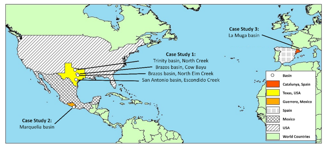
For all three case studies, the coupled hydrological-hydraulic distributed modelling was performed using Iber [47] version 3.1, a 2D free-surface numerical modelling initially developed for hydrodynamic and sediment transport purposes [47,48,49]. Currently, it includes several calculation modules [50,51,52,53,54,55,56,57], in particular, one for the simulation of the hydrological processes of rainfall-runoff transformation—including infiltration losses—fully integrated with the overland flow propagation [25,58,59].
Iber solves the 2D Shallow Water Equations (2D-SWE) using a conservative scheme based on the Finite Volume Method (FVM) on a structured or/and unstructured mesh of triangles and/or quadrilaterals. It uses the Roe scheme [60], which consists of the Godunov method together with Roe Approximate Riemann Solver [33].
The shear stress terms due to friction are generally incorporated in the SWE via the concept of the friction slope. This term expresses the contribution of the momentum change due to the energy dissipation produced by flow-boundary interactions as well as by a sub-grid of obstructions and by the losses due to the flow turbulence if, as it is generally done in coupled hydrological-hydraulic distributed modelling, no turbulence model is used. The friction slope ( S o ) is calculated using the Manning formula, which, in 2D, results in the following equations for the X and Y directions:
S o , x = n 2 U x U h h 4 / 3 S o , x = n 2 U y U h h 4 / 3
where n is the Manning roughness coefficient; U x and U y are the two components of the depth averaged velocity vector in X and Y direction, respectively; U is the modulus of the flow velocity; and h is the depth.
The DHD numerical scheme [25], developed ad hoc for hydrological modelling purposes, was used in all simulations with Iber. Briefly, this scheme merges the hydrostatic pressure gradient with the bed slope in a single term that depends on the free surface gradient. With this approach, when the free surface is horizontal, an exact balance between the bed slope and the hydrostatic pressure gradient is obtained naturally. As a result, more stable, efficient, and faster simulations (up to 1.5-times) are achieved as compared with other traditional FVM schemes [25,58,59].
Two additional options were also used in the simulations. On the one hand was an option that removes local depressions generated during the discretisation process along the flow path [61]. This tool is based on the technique proposed by Jenson and Domingue [62] in which each depression is refilled considering the lowest elevation of its neighbour cells. The application of this methodology is convenient even if the Digital Terrain Model (DTM) was previously treated with a Geographical Information System (GIS) software due two factors: (1) common GIS tools obtain the flow paths based on the connections between cells through their edges defined by the vertices, while the FVM uses the cells elevation to compute the flow; and (2) the topographical discretisation in the numerical model can use elements larger than the DTM raster cell size, and in the obtention, new depressions might be generated. Thus, this option ensures a proper definition of the flow path to work with the FVM whilst avoiding spurious depressions. On the other hand, to handle the transition from wet to dry conditions, and vice versa, Iber implements a wet-dry method by defining a water depth threshold ( ε w d ) below which a cell is considered to be dry. Low values of ε w d , such as 0.0001 m, as used herein in all cases, guarantee mass conservation and improve rainfall-runoff transformation as well as overland flow propagation [63].
Other particular parameters, as well as the numerical discretisation, are detailed in the description of each case study and in the Supplementary Material.

3. Case Studies

The role of the Manning coefficient roughness in the numerical modelling of the overland flow, performed with coupled hydrological-hydraulic distributed numerical models, was addressed, not referring to specific case studies around the world but to the numerical strategy performed. To that end, well documented studies that analyse the hydrological response of a basin were used from different points of views.
In Case Study 1, theoretical aspects related to the definition of the time of concentration and the role of the bottom roughness on the hydrological response were analysed. In Case Study 2, a distributed numerical model was calibrated by varying the roughness coefficient to fit the results to the hydrograph resulting from an aggregated model forced with synthetic hyetographs based on historical data. For that purpose, the parameters involved in the aggregated model were determined following the local administration recommendations. Finally, in Case Study 3, four different well-documented rainfall events in a monitored and regulated basin were used to force a distributed model aiming to analyse the role of the roughness coefficient in the overland propagation. The roughness coefficient was calibrated to adjust the simulated water elevation to the observed one during each event. A total of six basins, with different topographic and hydrologic characteristics, were analysed (Figure 1).

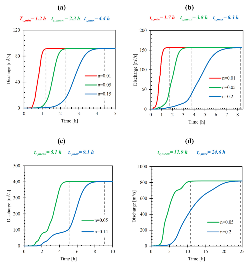
3.1. Case Study 1: Adjustment of the Roughness Coefficient Based on the Time of Concentration

In Case Study 1, the hydrological behaviour of four basins presented by Grimaldi et al. [10] is analysed. The four basins, located in USA, are: Brazos basin (Cow Bayu), San Antonio (Escondido Creek), Trinity basin (North Creek), and Brazos basin (North Elm Creek). Table 1 summarizes the main geometric characteristics. In Brazos (Cow Bayu) and Sant Antonio, there are large urban areas and both basins are regulated by a reservoir located at their lower parts. Trinity basin is a semi-rural area with five reservoirs that play a significant role in their hydrological behaviour. Finally, the largest basin, Brazos (North Elm Creek), is located in a rural area with two reservoirs (see Figure S1).
In this case study, a distributed coupled model was built for each basin using Iber. Details of the parameters and structure of the numerical models are described in the Supplementary Material. No aggregated hydrological modelling was used.
The numerical models were operated with constant rainfall intensities of infinite duration, analysing the output hydrographs (S-shaped). The required time for the hydrograph to stabilize to constant discharge, i.e., the time for the basin to achieve a stationary state, should coincide with the time of concentration if the WMO definition [14] is adopted. For the adjustment of the roughness coefficients based on t c , the six common expressions used by Grimaldi et al. [10], plus the Témez [17] formula commonly used in Spain, were selected. At this point, the question of ambiguity on the concept and formulas to estimate t c arises again as pointed out by Beven [12] and commented upon in the introduction. If the variable used to compare methodologies is the time the S-curves need to stabilize, but the formulas used to estimate the t c are empirically derived using the SCS-UH method or other similar means, there is a conceptual discrepancy as explained by Beven [12].
The different formulas used to estimate t c together with the results are presented in Table 2. It also shows the minimum, maximum, and mean values of the time of equilibrium that are going to be compared with the results of the distributed method.

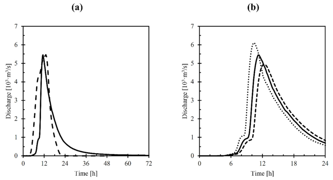
3.2. Case Study 2: Adjustment of the Roughness Coefficient Based on the Peak Time and Discharge from Aggregated Hydrological Models

Case Study 2 corresponds to the Mexican basin called Marquelia, located in the Guerrero region (Figure 1). The basin precipitation is monitored by eight rainfall gauge stations within or near it, and a hydrometric station at the outlet (see Figure S3a). The area of the Marquelia basin is 1016 km2 and its mean slope is 0.75%. Land uses are characterized by large extensions of secondary vegetation (48.51%) and forested (24.23%) areas. Other areas are covered by rivers (10.70%), pasturelands (10.60%), and rainforest agriculture extents (5.42%). According to the World Reference Base for Soil Resources [67], the basin edaphology is mainly composed of large areas of regosol (71%) and other types of soil such as phaeozem (11.3%) and cambisol (9.6%). From the land uses classification, a Curve Number (CN) of 76.7 was estimated as an area weighted average value in the whole basin.
Historical rainfall data was used to generate synthetic hyetographs associated with a 50-years return period (T50). Alternate block synthetic hyetographs [16] for a T50 event were calculated for each rain gauge station using the Intensity-Duration-Frequency (IDF) curves [68] and the time of concentration of 12.5 h resulting from the application of the Kirpich formula. Historical data of annual maximum precipitation were corrected, as proposed by Campos-Aranda [69], to account for the effect of using a fixed observation time-interval [70] and the non-uniformity of rainfall in the whole area of the basin.
On one hand, the output hydrograph was first calculated with aggregated modelling using HEC-HMS. The basin was discretized in seven subbasins. In each one, t c was estimated with Kirpich formula and t l a g as 0.6 t c . The subbasins were connected by three river reaches where the flow was propagated using the Muskingum routing method [16].
On the other hand, Iber was used for coupled hydrological-hydraulic distributed modelling. In this case, the terrain roughness was calibrated to adjust the hydrological behaviour (peak time and peak discharge) to that of the aggregated model. Six different Manning coefficient ( n ) values related to the land uses distribution of the basin (see Figure S3b) were used. All information regarding the topography, land uses, and precipitation data are presented in the Supplementary Material.

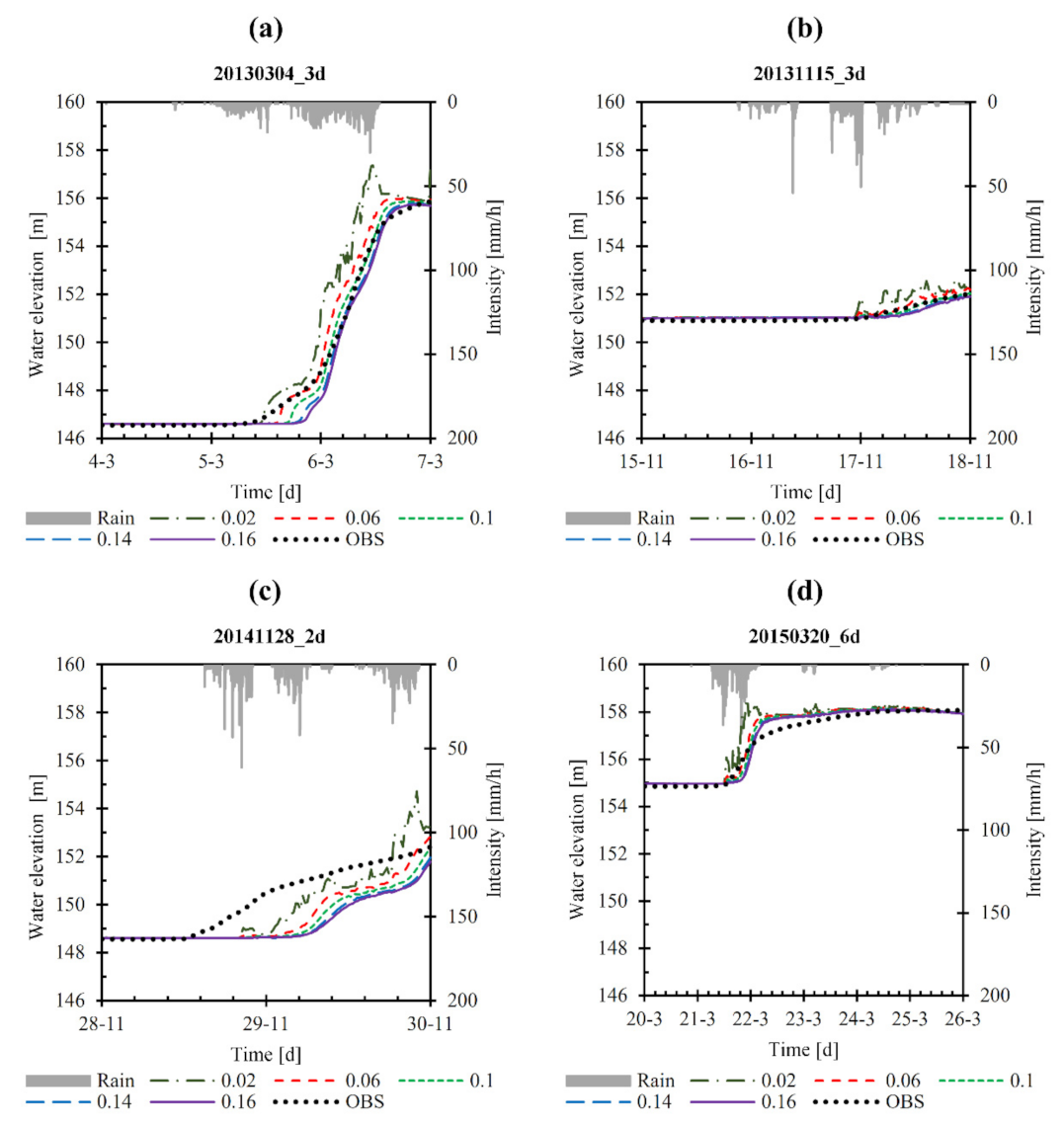
3.3. Case Study 3: Adjustment of the Roughness Coefficient Based on Observed Storm Events

Case Study 3 focuses on La Muga basin (Spain). Four well-documented rainfall events [58,59,71] were used to assess the hydrological response of the basin by varying the roughness coefficient values in the distributed model.
The study area consists of the upper part of La Muga basin, which has an extension of 181.2 km2 and a reservoir at the outlet of 61 hm3 of storage capacity. Weather conditions of the basin are characterized by a wide variability of the rainfall regime, which is influenced by marine conditions with small thermal as well as rain variations [72]. Extreme weather conditions—such as heavy rain events with high precipitation intensities and water accumulations concentrating in a few days or hours, and water scarcity associated to long dry-weather periods—are typical of the area [73,74].
A land use analysis [75] revealed that the basin is mainly covered by large forest extensions (92.5%), while a terrain characteristics analysis indicated a low permeability and underground storage capacity [72]. Thus, the hydrological response of the basin can be characterized with a unique land use and soil texture.
In the same way as for Case Study 2, the NRCS-CN method was applied to transform rainfall into runoff. Previous studies [58,59,71] allowed determining the CN value as a function of each studied rainfall event and the soil moisture antecedents evaluated with remote sensing [76,77]. The resulting CN values varied from 50 to 81. The four events were labelled with the starting date (year/month/day) and the duration in days as follows: 20130304_3d, 20131115_4d, 20141128_2d, and 20150320_6d. Table 3 summarizes the cumulated rainfall for each event, the maximum registered rainfall intensity, and the CN value. A more extended description of these events is detailed in the Supplementary Material.
Based on the uniformity of land uses and soil characteristics in the basin, a unique Manning coefficient value was used. The model calibration was performed by comparing the calculated and observed water elevation at the Boadella reservoir dam, located at the basin’s lower end (see Figure S5).

4. Results

4.1. Case Study 1

Four distributed hydrological models were built, one for each of the four basins. The domain was discretized with a calculation mesh of a regular grid generated directly using the DTM data, being quadrilateral elements with sides of approximately 9.5 m. A constant rainfall intensity of 25 mm/h was assigned to the whole domain. In this case, no infiltration losses were considered; thus, the rainfall intensity was considered to be effective precipitation. The value of the Manning coefficient ( n ) was varied from 0.01 to 0.2 s/m1/3, in intervals of 0.01 s/m1/3. The purpose was to obtain the best approximation for the minimum, the maximum, and the mean times of concentration ( t c ) calculated with the empirical formulas (Table 2). The maximum discharge generated with the aforementioned rainfall intensity is, in this case, a constant discharge. For the estimation of t c , the discharge was considered to be constant when its variation between two consecutive results time steps was lower than 0.1% of the discharge. Results time steps of 60 s were used.
Figure 2 shows the simulated hydrograph in each basin for the selected Manning coefficients, together with its value. All of them are consistent with the S-curve shape characteristic of the rational method [16,78], which stabilizes at the same value obtained with the rational method, i.e., the product of the effective rain intensity and the basin area (see Table S1). For the Brazos (Cow Bayu) (Figure 2a) and San Antonio (Figure 2b) basins, a very low value of the Manning coefficient (0.01 s/m1/3) was needed for the S-curve to fit with the minimum t c , which, in this case, corresponds to the Kirpich formula. In Trinity (Figure 2c) and Brazos (North Elm Creek) (Figure 2d) basins, it was not possible to reproduce the minimum t c without considering any friction since the hydrograph needed more time than the minimum t c to stabilize. For this reason, they are not plotted in Figure 2. This induces the thought that the Kirpich formula, the one that provides such minimum values, is quite unrealistic for these basins, as water propagation is slower even with no friction. This is in agreement with the assertion of Michailidi et al. [11] that “the Kirpich formula is a special case of a very general expression that is valid under very limited conditions” and that this formula was obtained for basins where channel flow was predominant.
The particular shape of each S-curve depends on the geometry and hydrological behaviour of each basin. The shape of the basin and the river network play an important role not just in the hydrograph definition, but also the drainage area. For the analysed basins, the smaller ones (Figure 2a,b) follow a more standard S-shaped hydrograph; in contrast, in the bigger ones (Figure 2c,d), the contribution of each part of the basin is most clearly appreciated and the hydrographs’ shape differ more from a smooth S-shape. In particular, the hydrographs of Trinity basin (Figure 2c) show some more flat areas (around 2 h for n = 0.05 s/m1/3 and between 3 and 5 h for n = 0.14 s/m1/3) after an initial rapid discharge increase, which can be attributed to the effect of small basins having reached their maximum discharges.
Numerical results show a wide range of the Manning coefficient, from values lower than 0.01 up to 0.2 s/m1/3 in order to achieve similar responses of the basin to those obtained by common time of concentration formulas and an aggregated model. As expected, a low value of the Manning coefficient provides faster response, while high values in a slower runoff advance. It is worth mentioning that a unique roughness coefficient value was used all over the basin; thus, a more detailed roughness discretisation would result in higher values at hillsides and areas outside of the hydrographic network, and lower ones in rivers and floodplains.

4.2. Case Study 2

The hydrological analysis of the Marquelia basin was performed first with an aggregated approached using HEC-HMS and the UH method, and then with a distributed model using Iber. The first model, built following the existing recommendations in Mexico, was taken as the reference for adjusting the roughness coefficients in the second one. In this, the domain was discretised with seven subbasins and three reaches. The time of concentration for each subbasin, t c , i , was determined by the Kirpich formula. The Muskingum method was used as the routing method [16], the parameters—K and χ—ere estimated following the recommendations of Fuentes et al. [79]. A more extended description is detailed in the Supplementary Material.
On the other hand, for the distributed approach, an irregular calculation mesh made of triangular elements, between 100 and 500 m of side, was built. Smaller elements were used in the river network while greater ones were used on the hillsides, aimed at optimizing the computational time and results accuracy balance. The topographical data used was the 15 m cell size DTM provided by the Mexican National Institute of Statistics and Geography, INEGI [80]. The Manning coefficients that associated the spatial distribution of the land uses map (Figure S3b) were calibrated. Additional information of the model discretisation is detailed in Supplementary Material.
The values of the Manning roughness coefficient that provide the best adjustment in terms of peak discharge are depicted in Table 4. They range from 0.069 s/m1/3, corresponding to urban settlements, to 0.207 s/m1/3 corresponding to forested area. All these values widely exceed the traditionally recommended values for hydraulic computations in artificial or natural channels and floodplains areas [38,39,40,81,82,83].
Figure 3a plots the hydrographs resulting from the aggregated approach (dashed line) and the distributed approach (continuous line). The peak discharge and the hydrograph volume differ, in absolute value, by less than 0.2% and 3%, respectively, being in both cases lower in the ones obtained in the distributed approach. The aggregated model provides a faster hydrological response with almost two partial peaks discharges at 8.5 h and 11.5 h, while the maximum peak discharge is produced 1.6 h after the one obtained by the distributed model. In this sense, the distributed model also produces a partial peak at around 8.5 h but with a lower discharge.
Despite the whole basin being split into seven subbasins and three river-reaches, the hydrological response of this semi-aggregated model does not represent the basin response as accurately as the distributed one. In this case, the shape of the hydrograph is clearly influenced by the rainfall-runoff method (UH). This is especially denoted in the generation of a partial peak during the first hours and a fast decay of recession curve after the maximum peak discharge, the discharge being zero after 27 h.
On the other hand, the distributed numerical modelling based on the 2D-SWE solution, which allows considering the full topographical and land uses characteristics of the basin and subbasins, provides more accurate results for the hydrograph shape. A sensitivity analysis was carried out by considering variations of ± 20% in the Manning roughness coefficients (Table 4). Figure 3b also presents the resulting hydrographs of this analysis (dotted and dashed lines), increasing the peak discharge while decreasing the time of the peak when the roughness coefficient decreases, and vice versa. It is worth noting that the peak discharge varies from −9.5% (+20% of n values) to 11.9% (−20% of n values), while the time of the peak and the hydrograph volume vary by exactly ± 8.8% and ± 0.5%, respectively. Thus, variations on the roughness coefficient are directly related to the time when peak discharge is produced, but the value of the peak discharge is not proportionally increased/reduced due to this variation.

4.3. Case Study 3

The model of La Muga basin was based on a spatial discretisation of triangular mesh elements with variable size that were finer in rivers (20 m) and coarser in hillslopes (200 m), constructed from a high resolution DTM of 2 × 2 m cell size [84]. As normal river discharge is small in comparison with the bankfull, the DTM, from a LiDAR flight, is a good approximation of the riverbed geometry.
The model was operated with variations on the Manning roughness coefficient ( n ), from 0.02 to 0.16 s/m1/3 with steps of 0.02 s/m1/3, resulting in different hydrological responses. The computed water elevation in the reservoir at the basin outlet was compared with the field observations along the events and at the end of each one. Figure 4 shows the simulated water elevation for the four rainfall events analysed.
In Figure 4a, the results of 20130304_3d event are shown, which concentrates on the rainfall during day 2 and the first-half of day 3. In it, the simulated water elevation at the end of the event is similar to the observed one for all scenarios, with relative errors being less than 1.5%, and the value of n being 0.1 s/m1/3—one that achieves the best adjustment (0.005% of error). For this event, significant differences on the arrival time of the flood can be observed, with a time gap of around 12 h between the hydrographs corresponding to the minimum and maximum n values. The evolution of the water elevation during the second-half of day 2 clearly shows faster hydrological responses for low values of n .
Figure 4b shows the results of the simulations for the 20131115_3d event. The simulations fit well with the observations in terms of final water resources (volume of water in the reservoir), with relative errors being less than 0.2%. In this case, where rainfall intensities around 50 mm/h were recorded in the middle of day 2 and at the beginning of day 3, the evolution of the water elevation was not very sensible to variations of the Manning coefficient, especially for n values greater than 0.06 s/m1/3.
The 20141128_2d event (Figure 4c) shows the worst adjustment of all events in the reproduction of the water elevation evolution, but, by contrast, it also achieves a good performance in terms of water resources at the end of the event (relative error less than 0.6%). In this case, the three peaks of rainfall intensity registered generated an almost constant increment of water resources stored in the reservoir; however, the numerical model did not reproduce this trend, probably because in the model the rainfall distribution was considered to be homogeneous all over the basin, unlike the real case [59]. Only for a Manning coefficient between 0.06 and 0.12 s/m1/3, the water elevation at the end of the event shows a good adjustment with relative error being less than 0.16%.
Finally, in the 20150320_6d event shown in Figure 4d, which lasted 6 days, although more than 80% of the rainfall was concentrated during day 2, the numerical model reproduced well the water resources volume at the end of the event, with relative error being less than 0.09%. In this case, the evolution of the water elevation was similar to the observations, but for a slightly sharper increment of the water elevation between day 2 and 3. This fact is probably because the rainfall registered at the gauge station overestimated the real precipitation as pointed out by Sanz-Ramos [59].
The results show that the dependency of the time arrival of the water front to the Manning coefficient values is more evident for low n values (less than 0.08 s/m1/3). In general, the hydrological response of the model is more sensible for low values of n than for high ones, especially from the point of view of water resources. As expected, low values of n produce larger overland flow discharges in shorter times.
No remarkable differences were observed in the model results for values of n greater than 0.08 s/m1/3. The precision of the results is aligned with the assumption of a unique Manning roughness coefficient value for the whole catchment, which in this case, was appropriate for hydrological purposes. On the other hand, for values of n in the lower range, oscillations on the water surface elevation appear.
Several indicators were used to assess the adjustment between the observations and the simulated results—root-mean square error (RMSE), mean absolute error (MAE), and the coefficient of determination (R2). Table 5 summarizes the performance of the model for the four rainfall events in terms of these indicators. A good adjustment is seen for 20130304_3d and 20131115_3d events, with low values of MAE and RMSE, but also with high values of R2. The performance of 20141128_2d event is, in general, the poorest—the simulated water resources are clearly underestimated during almost all the event. In contrast with the other events, as the hydrological response is slower in comparison with the observations, the indicators show the best adjustments are for low values of n . Finally, the 20150320_6d event presents the worst R2 values. A peer-to-peer results analysis (RMSE and MAE) reveals that the model has, in general, a good adjustment, especially for values of n greater than 0.06 s/m1/3.
It is worth noting that the influence of the rainfall antecedents (arrival time of the water front) and the spatial distribution of the precipitation (non-expected increase of water elevation at the end of the episode) can condition the previous statistics. Nevertheless, from the previous considerations, it can be asserted that the performance of the model is, in general, good enough for the purpose of the simulations.

5. Discussion

On the roughness coefficient values and their effect on the hydrological response
In free surface hydraulic numerical modelling, shear terms due to friction express the contribution of the momentum change due to the energy dissipation produced not only by flow-boundary interactions, but also by sub-grid turbulence if, as is generally done, no turbulence model is used. Since for hydrological purposes, the effect of turbulence is generally neglected, only the friction of the fluid with the terrain represents the energy dissipation. I.e., in 2D-SWE-based coupled hydrological-hydraulic distributed numerical modelling, the bottom roughness conditions not only the flow routing in the river network, but also the overland flow on the areas where the rainfall-runoff process takes place (hillsides).
Hence, the Manning roughness coefficient can be considered as a “property” of the terrain material where the overland flow is propagated. In 2D-SWE-based models, anisotropic properties of the shear stress terms (see Equation (1)) can be due not only to the velocity field but also to the Manning coefficient [85,86,87]. Thus, Manning coefficient could be considered as a vector to represent the anisotropic properties of the terrain (Equation (2)), where n x and n y are the two components of the Manning coefficient vector in X and Y direction, and n its modulus.
S o , x = n x n U x U h h 4 / 3 S o , x = n y n U y U h h 4 / 3
However, there is no strong evidence that confirms that the Manning’s anisotropy should be considered in hydrological studies because the overland flow usually propagates in the same direction, especially over the hillsides where the rainfall-runoff process is generated. By contrast, the time-space variability of the Manning coefficient, including the dependency of the main hydraulic variables (depth and/or velocity), must be considered in general; the coupled hydrological-hydraulic distribute modelling is the unique numerical strategy that can deal with this.
On the other hand, despite the fact that in distributed numerical modelling the topographical discretisation of the domain is more accurate than for aggregated numerical modelling, the hydraulic behaviour of the water for very low depths (millimetric scale or lower) is not properly reproduced by the solution of the SWE. In this situation, the flow scale is in the same order of magnitude of the terrain particles scale, and the fluid tends to move more slowly than for larger river-like flow scales. Thus, in order to avoid too-fast hydrological responses, the bottom roughness must be increased in relation to the values used in common hydraulic situations. This explains why high values of the bottom roughness, the Manning coefficient value ( n ), are required in Case Study 2 and Case Study 3 to obtain a good performance of the numerical model from a hydrological point of view. In contrast, very low values of n are needed in Case Study 1 for an accurate adjustment of the time of concentration obtained with the Kirpich formula. A n value of 0.01 was needed to reach a similar t c in Brazos and San Antonio basins, whereas in the other basins, this value was even lower than the previous one. This is in line with various authors’ discussions on the appropriateness of the Kirpich formula in situations other than those for which it was obtained [10,11,12].
The generally high values of the roughness coefficient obtained in the three case studies are far from the values extensively used for hydraulic purposes in flood routing [40], but are within the range of values generally found in the literature for hydrological purposes [26,30,31,42,88,89,90,91], especially for hillslopes and flood plains, where the rainfall-runoff process predominates.
On the role of the domain discretisation in the basin hydrological response
In general, coarse meshes provide faster simulations but poorer resolution and accuracy. In contrast, finer meshes provide more accurate results while the computational effort increases. Thus, practitioners must deal with achieving a proper balance to obtain good results with a reasonable computational effort.
Improvements in topographical and rainfall data acquisition and the increase of the computational capacity, in particular those related to Graphical Processing Unit (GPU) computing in particular [89,92,93,94], are continuously leading to the advance of the numerical modelling, especially in hydrology. This new framework pushes modellers to generate increasingly detailed coupled hydrological-hydraulic distributed numerical models, even using, if necessary, the full information of the DTM (as shown for example in Case Study 1) as the computation mesh and distributed rainfall data. However, mesh resolution affects the model hydrological response (peak discharge) and rainfall intensity affects the value of the time of concentration of the basin.
To illustrate the last two facts, a double sensitivity analysis was carried out on Marquelia basin. The results show that the peak discharge increases when the number of elements of the numerical model also increases (Figure 5a). An asymptotic trend towards 7000 m3/s is observed for calculation meshes with more than 1.9 million elements. This peak discharge increment is probably due to the better representation of the topography, in general, as well as the better definition of the river-channel, in particular, which improve the flow propagation representation. This last domain discretisation (1.9 M elements) represents approximately 19 elements per ha, which is still far from the values of flood studies where more than 1000 elements per ha is quite common [95].
On the other hand, the time of response of a basin depends not only on the Manning coefficient but also on rainfall intensity [11]. Higher rainfall intensities imply shorter hydrological responses, i.e., the time of concentration becomes smaller. In this case, the t c was estimated as the time from the end of the excess rainfall to the point of inflection of the hydrograph where the recession curve begins [96]. Using the same model discretisation for Case Study 2 and varying the return period of the rainfall hyetograph from 2 to 10,000, it is possible to observe how the time of concentration tends to a constant value of around 15 h for the statistically less frequent events (Figure 5b). This fact is aligned with Grimaldi et al. [10], who suggest that t c becomes quasi-invariant with respect to the rainfall intensity for flood events with a high return period and who also signalled the time of concentration dependency with the cell-size of the DTM when using NRCS method. Thus, the use of coupled hydrological-hydraulic distributed models, where the time of concentration is no longer part of the modelling process, might reduce the uncertainties related to the rainfall-runoff processes.
On the numerical approach
Currently, there are three different strategies to carry out an overland flow analysis—conceptual, aggregated, and distributed. Conceptual and aggregated approaches are the simplest and are based on the main basin characteristics, such as the extent, main river length, main river slope, and soil characteristics to estimate the rainfall-runoff threshold, etc., and summarize all hydrological processes for the estimation of the peak discharge associated to a rainfall intensity (e.g., Rational Method).
Aligned with the evolution in the state of the art of applied hydrology, the aggregated models integrate the previous conceptual models into numerical models. They are tools based on the physics of the problem that, by integrating empirical formulas for overland processes, first allowed simulating rainfall events, groundwater interactions, flow routing, etc. These models are still widely extended because they are fast, robust, and conceptually simple. However, as for other numerical tools, to achieve good results they must be calibrated. In them, one of the main parameters to calibrate is the time of concentration ( t c ), which can be estimated by empirical formulas of one or the other authors. Additionally, practitioner’s expertise is crucial to determine the number of subbasins to define the rainfall-runoff and routing methods, etc.; thus, in all of these processes, the error derived from selecting one or the other parameter is propagated till the final result: the hydrograph.
Finally, the more recently-developed distributed models, and in particular the coupled hydrological-hydraulic 2D-SWE-based tools, provide more detailed hydrologic as well as hydraulic results. In this case, the practitioner’s expertise may be somewhat less relevant because there are less parameters to calibrate; in fact, only the terrain roughness. The domain discretisation is also important to achieve suitable results. It plays a similar role to the subbasins’ definition in aggregated approaches but, in this case, the modeller has only to decide the mesh element size (minimum, maximum, or mean) and not how many subbasins/reaches the domain must be divided into.
As shown along the document, the value of the terrain roughness in 2D-SWE-based distributed approach is usually out of the range for hydraulic purposes as overland flow tends to move more slowly than when the flow is propagated along a river. Additionally, a distributed approach allows considering the terrain properties and characteristics element by element.

6. Conclusions

The bottom roughness, evaluated here via the Manning roughness coefficient, is one of the main calibration parameters for hydrological modelling based on coupled hydrological-hydraulic distributed numerical tools. The mesh resolution also plays an important role on the overland flow propagation, especially on the definition of the peak discharge associated to a rainfall event.
Due to the ambiguities in the definition of the time of concentration and the high dispersion of the values obtained with different formulae, the adjustment of the Manning coefficients with the time of concentration is uncertain and of little practical interest. The Manning coefficients that have to be used in coupled hydrological-hydraulic modelling in order to reach a time of concentrations similar to those obtained by empirical formulas show an extremely high dispersion. Moreover, they are out of the common range of values used for hydraulic purposes. In particular, it was shown that for the Kirpich formula, the required value of the roughness coefficient for the time of concentration adjustment is close or lower than 0.01 s/m1/3, which would correspond to the hydraulic value for very smooth material, much different from those existing in natural basins.
The global picture of the presented results shows that higher values of the Manning coefficient than those commonly used for hydrodynamic purposes are required when computing the overland flow of a basin using coupled hydrological-hydraulic distributed numerical tools. This is because the roughness coefficient must integrate the momentum change due to the energy dissipation produced not only by flow-boundary interactions, but also by sub-grid turbulence, in the river network and in the areas where the rainfall-runoff is mainly generated (hillsides).
In coupled hydrological-hydraulic distributed models, the roughness coefficient has a clear role on the arrival time of the water front, playing a similar role like the lag time in conceptual and aggregated models. However, there is no exact relation of roughness values with commonly used hydrological parameters, which means that trying to estimate the roughness coefficient by comparing distributed and aggregated model results is not a good idea. From the authors’ points of view, there is still little experience, though increasing rapidly, in the verification of coupled hydrological-hydraulic distributed models; thus, the recommendation would be to use this approach in cases with enough data for model calibration and validation while experience in this kind of model continues to increase and eventually more recommendations and guidelines appear.

Supplementary Materials

The following are available online at https://www.mdpi.com/article/10.3390/w13233433/s1, Figure S1: Case Study 1. Topographical description of the four basins: (a) Brazos, Cow Bayu; (b) San Antonio, Escondido Creek; (c) Trinity, North Creek; (d) and Brazos, North Elm Creek. Reservoirs, when exists, are depicted in with a blue polygon. Geographical coordinates of the outlet (red dot) are referenced in UTM Zone 14N, Figure S2: Case Study 1. Example of the levelling process of the terrain in the area that represents a dam in Trinity basin. Calculation mesh of Iber before (a) and after (b) the levelling process, Figure S3: Characterization of the Case Study 2: (a) Topographical map of the basin, influence area of the most closed rain gauges stations (green stars) according to a Thiessen polygon discretization (black lines) and location of the hydrometric station (yellow pentagon); (b) Map of land uses and location of the outlet (red dot), georeferenced in UTM Zone 14N; (c) Map of soil edaphology; and (d) Map of Curve Number according to SCS-CN method, Figure S4: Case study 2. Synthetic hyetographs corresponding to a 50-years return period for the eight most closed rainfall station to Marquelia basin, Figure S5: Case Study 3. Topographical map of the upper part of La Muga basin and location of the gauge station (yellow pentagon) and the outlet (red dot), which is referenced in UTM Zone 31N, Figure S6: Case Study 3. 5-minutal time-resolution hyetographs rainfall intensity (grey bar) and outlet discharge from the reservoir (black line), Table S1: Maximum discharge (in m3/s) for the four basins of the Case Study 1 estimated by the Rational Method for a constant rainfall intensity of 25 mm/h, Table S2: Characteristics of the discretization of the Marquelia basin and parameters of the aggregated numerical approach, Table S3: Spatial characteristics of the land uses of the Marquelia basin and Manning roughness coefficient best fit to the 50-years return period synthetic hydrograph.

Author Contributions

Conceptualization, M.S.-R., E.B. and J.L.A.-H.; methodology, E.B.; software, F.G.-E., M.S.-R. and G.O.; formal analysis, M.S.-R.; resources, F.G.-E., E.B. and J.L.A.-H.; data curation, F.G.-E., M.S.-R. and J.L.A.-H.; writing—original draft preparation, M.S.-R. and F.G.-E., G.O., E.B. and F.G.-E. writing—review and editing, E.B. and M.S.-R.. All authors have read and agreed to the published version of the manuscript.

Funding

This research was partially funded by the Pyrénées-Méditerranée Euroregion (European Commission), grant number INTERREG AECT-2014/PGRI-EPM, and the CONACYT (Mexico) that granted the scholarship to F.G.-E. for a research stay at Flumen Institute during his master studies.

Institutional Review Board Statement

Not applicable.

Informed Consent Statement

Not applicable.

Data Availability Statement

Data available in a publicly accessible repository that does not issue DOIs.

Acknowledgments

The authors would like to thank the Agència Catalana de l’Aigua (ACA) and Servei Meteorològic de Catalunya (SMC) that provided the “Rainfall and water level” data for Case Study 3, as well as its advisement during the project. F.G.-E. also gives thanks to CONACYT for the grant received to do an internship at Flumen Institute.

Conflicts of Interest

The authors declare no conflict of interest. The funders had no role in the design of the study; in the collection, analyses, or interpretation of data; in the writing of the manuscript; or in the decision to publish the results.

References

  1. Fonseca, A.R.; Santos, M.; Santos, J.A. Hydrological and flood hazard assessment using a coupled modelling approach for a mountainous catchment in Portugal. Stoch. Environ. Res. Risk Assess. 2018, 32, 2165–2177. [Google Scholar] [CrossRef]
  2. Kron, W. Flood Risk = Hazard + Values + Vulnerability. Water Int. 2005, 30, 58–68. [Google Scholar] [CrossRef]
  3. ISDR Global Assessment Report on Disaster Risk Reduction; United Nations: Geneva, Switzerland, 2009; ISBN 978-92-1-332019-8.
  4. Fraga, I.; Cea, L.; Puertas, J.; Mosqueira, G.; Quinteiro, B.; Botana, S.; Fernández, L.; Salsón, S.; Fernández-García, G.; Taboada, J. MERLIN: Una nueva herramienta para la predicción del riesgo de inundaciones en la demarcación hidrográfica Galicia-Costa. Ing. Agua 2021, 25, 215. [Google Scholar] [CrossRef]
  5. Thiemig, V.; Bisselink, B.; Pappenberger, F.; Thielen, J. A pan-African medium-range ensemble flood forecast system. Hydrol. Earth Syst. Sci. 2015, 19, 3365–3385. [Google Scholar] [CrossRef] [Green Version]
  6. Mure-Ravaud, M.; Binet, G.; Bracq, M.; Perarnaud, J.-J.; Fradin, A.; Litrico, X. A web based tool for operational real-time flood forecasting using data assimilation to update hydraulic states. Environ. Model. Softw. 2016, 84, 35–49. [Google Scholar] [CrossRef]
  7. Alvarez-Garreton, C.; Ryu, D.; Western, A.W.; Su, C.-H.; Crow, W.T.; Robertson, D.E.; Leahy, C. Improving operational flood ensemble prediction by the assimilation of satellite soil moisture: Comparison between lumped and semi-distributed schemes. Hydrol. Earth Syst. Sci. 2015, 19, 1659–1676. [Google Scholar] [CrossRef] [Green Version]
  8. Beven, K. Rainfall-Runoff Modelling. The Primer; John Wiley & Sons, Ltd.: Chichester, UK, 2012; ISBN 9780470714591. [Google Scholar]
  9. Paudel, M.; Nelson, E.J.; Downer, C.W.; Hotchkiss, R. Comparing the capability of distributed and lumped hydrologic models for analyzing the effects of land use change. J. Hydroinform. 2011, 13, 461–473. [Google Scholar] [CrossRef]
  10. Grimaldi, S.; Petroselli, A.; Tauro, F.; Porfiri, M. Time of concentration: A paradox in modern hydrology. Hydrol. Sci. J. 2012, 57, 217–228. [Google Scholar] [CrossRef] [Green Version]
  11. Michailidi, E.M.; Antoniadi, S.; Koukouvinos, A.; Bacchi, B.; Efstratiadis, A. Timing the time of concentration: Shedding light on a paradox. Hydrol. Sci. J. 2018, 63, 721–740. [Google Scholar] [CrossRef] [Green Version]
  12. Beven, K.J. A history of the concept of time of concentration. Hydrol. Earth Syst. Sci. 2020, 24, 2655–2670. [Google Scholar] [CrossRef]
  13. Mulvany, T.J. On the use of self-registering rain and flood gauges in making observations of the relations of rainfall and flood discharges in a given catchment. Proc. Inst. Civ. Eng. Irel. 1851, 4, 18–33. [Google Scholar]
  14. W.M.O. International Glossary of Hydrology. Report No. 385; World Meteorological Organization (W.M.O.): Geneva, Switzerland, 1974. [Google Scholar]
  15. NCRS Hydrology. National Engineering Handbook; US Department of Agriculture: Washington, DC, USA, 1972. [Google Scholar]
  16. Chow, V.T.; Maidment, D.R.; Mays, L.W. Applied Hydrology; MCGRAW-HIL: New York, NY, USA, 1988; ISBN 9780071001748. [Google Scholar]
  17. Témez, J.R. Cálculo Hidrometeorológico de Caudales Máximos en Pequeñas Cuencas Naturales; Ministerio de Obras Públicas y Urbanismo, Dirección General de Carreteras: Madrid, España, 1978; ISBN 7433-457-8. [Google Scholar]
  18. Kirpich, Z.P. Time of concentration of small agricultural watersheds. Am. Soc. Civ. Eng. 1940, 10, 362. [Google Scholar]
  19. Mijares, A. Fundamentos de Hidrología de Superficie; Editorial Limusa, Grupo Noriega Editores: México D.F., México, 1998; ISBN 9681830148. [Google Scholar]
  20. CONAGUA. Manual de Agua Potable, Alcantarillado y Saneamiento: Drenaje Pluvial Urbano; Comisión Nacional del Agua. Naturales, Secretaría de Medio Ambiente y Recursos: Ciudad de México, México, 2016; ISBN 9786076260159. [Google Scholar]
  21. SCT. Estudios Hidráulico-Hidrológicos para Puentes: Manual de Análisis Hidrológicos; Secretaría de Comunicaciones y Transportes, Gobierno de México: Ciudad de México, México, 2000. [Google Scholar]
  22. Nanía, E.S.; Gomez-Valentín, M. Ingeniería Hidrológica, 2nd ed.; Grupo Editorial Universitario: Granada, España, 2014; ISBN 84-8491-636-7. [Google Scholar]
  23. Reed, S.; Koren, V.; Smith, M.; Zhang, Z.; Moreda, F.; Seo, D.J. Overall distributed model intercomparison project results. J. Hydrol. 2004, 298, 27–60. [Google Scholar] [CrossRef]
  24. Refsgaard, J.C. Parameterisation, calibration and validation of distributed hydrological models. J. Hydrol. 1997, 198, 69–97. [Google Scholar] [CrossRef]
  25. Cea, L.; Bladé, E. A simple and efficient unstructured finite volume scheme for solving the shallow water equations in overland flow applications. Water Resour. Res. 2015, 51, 5464–5486. [Google Scholar] [CrossRef] [Green Version]
  26. Caro, C.A. Modelación Hidrológica Distribuida Basada en Esquemas de Volúmenes Finitos. Ph.D. Thesis, School of Civil Engineering, Universitat Politècnica de Catalunya, Barcelona, Spain, 2016. [Google Scholar]
  27. Kim, J.; Warnock, A.; Ivanov, V.Y.; Katopodes, N.D. Coupled modeling of hydrologic and hydrodynamic processes including overland and channel flow. Adv. Water Resour. 2012, 37, 104–126. [Google Scholar] [CrossRef]
  28. Cea, L.; Garrido, M.; Puertas, J. Experimental validation of two-dimensional depth-averaged models for forecasting rainfall–runoff from precipitation data in urban areas. J. Hydrol. 2010, 382, 88–102. [Google Scholar] [CrossRef]
  29. Viero, D.P.; Peruzzo, P.; Carniello, L.; Defina, A. Integrated mathematical modeling of hydrological and hydrodynamic response to rainfall events in rural lowland catchments. Water Resour. Res. 2014, 50, 5941–5957. [Google Scholar] [CrossRef] [Green Version]
  30. Yu, C.; Duan, J. Simulation of Surface Runoff Using Hydrodynamic Model. J. Hydrol. Eng. 2017, 22, 04017006. [Google Scholar] [CrossRef]
  31. Nguyen, P.; Thorstensen, A.; Sorooshian, S.; Hsu, K.; AghaKouchak, A.; Sanders, B.; Koren, V.; Cui, Z.; Smith, M. A high resolution coupled hydrologic–hydraulic model (HiResFlood-UCI) for flash flood modeling. J. Hydrol. 2016, 541, 401–420. [Google Scholar] [CrossRef] [Green Version]
  32. Panday, S.; Huyakorn, P.S. A fully coupled physically-based spatially-distributed model for evaluating surface/subsurface flow. Adv. Water Resour. 2004, 27, 361–382. [Google Scholar] [CrossRef]
  33. Toro, E.F. Riemann Solvers and Numerical Methods for Fluid Dynamics; Springer: Berlin/Heidelberg, Germany, 2009; Volume 40, ISBN 978-3-540-25202-3. [Google Scholar]
  34. Beven, K. Changing ideas in hydrology—The case of physically-based models. J. Hydrol. 1989, 105, 157–172. [Google Scholar] [CrossRef]
  35. Jakeman, A.J.; Hornberger, G.M. How much complexity is warranted in a rainfall-runoff model? Water Resour. Res. 1993, 29, 2637–2649. [Google Scholar] [CrossRef]
  36. Barnes, C.J. The art of catchment modeling: What is a good model? Environ. Int. 1995, 21, 747–751. [Google Scholar] [CrossRef]
  37. Beven, K. How far can we go in distributed hydrological modelling? Hydrol. Earth Syst. Sci. 2001, 5, 1–12. [Google Scholar] [CrossRef]
  38. Chow, V. Open Channel Hydraulics; McGraw-Hill Education: New York, NY, USA, 2006; ISBN 9780750668576. [Google Scholar]
  39. Barnes, H.H. Roughness characteristics of natural channels. J. Hydrol. 1969, 7, 354. [Google Scholar]
  40. Arcement, G.J.G.J.J.J.; Schneider, V.R. Guide for Selecting Manning’s Roughness Coefficients for Natural Channels and Flood Plains; Paper 2339; 19. Books and Open-File Reports Section; U.S. Geological Survey, Federal Center: Denver, CO, USA, 1989. [Google Scholar]
  41. Kalyanapu, A.J.; Burian, S.J.; McPherson, T.N. Effect of land use-based surface roughness on hydrologic model output. J. Spat. Hydrol. 2009, 9, 51–71. [Google Scholar]
  42. Barnard, T.; Agnaou, M.; Barbis, J. Two Dimensional Modeling to Simulate Stormwater Flows at Photovoltaic Solar Energy Sites. J. Water Manag. Model. 2017, 25, 8. [Google Scholar] [CrossRef] [Green Version]
  43. USACE. Hydrologic Modeling System HEC-HMS. Technical Reference Manual; US Army Coprs of Engineers, Institute for Water Resources, Hydrologic Engineering Center: Dacis, CA, USA, 2000. [Google Scholar]
  44. USDA-SCS. SCS National Engineering Handbook, Hydrology, Section 4; US Department of Agriculture, Soil Conservation Service: Washington, DC, USA, 1972. [Google Scholar]
  45. USDA-SCS. National Engineering Handbook, Supplement A, Section 4, Chapter 10: Hydrology; US Department of Agriculture, Soil Conservation Service: Washington, DC, USA, 1985. [Google Scholar]
  46. USDA-NRCS. Part 630 Hydrology—Chapter 10. In National Engineering Handbook; US Department of Agriculture, Soil Conservation Service: Washington, DC, USA, 2004; p. 79. [Google Scholar]
  47. Bladé, E.; Cea, L.; Corestein, G.; Escolano, E.; Puertas, J.; Vázquez-Cendón, E.; Dolz, J.; Coll, A. Iber: Herramienta de simulación numérica del flujo en ríos. Rev. Int. Métodos Numér. Cálc. Diseño Ing. 2014, 30, 1–10. [Google Scholar] [CrossRef] [Green Version]
  48. Cea, L.; Bladé, E.; Corestein, G.; Fraga, I.; Espinal, M.; Puertas, J. Comparative analysis of several sediment transport formulations applied to dam-break flows over erodible beds. In Proceedings of the EGU General Assembly 2014, Vienna, Austria, 27 April–2 May 2014. [Google Scholar]
  49. Bladé, E.; Cea, L.; Corestein, G. Numerical modelling of river inundations. Ing. Agua 2014, 18, 68. [Google Scholar] [CrossRef]
  50. Anta Álvarez, J.; Bermúdez, M.; Cea, L.; Suárez, J.; Ures, P.; Puertas, J. Modelización de los impactos por DSU en el río Miño (Lugo). Ing. Agua 2015, 19, 105. [Google Scholar] [CrossRef]
  51. Cea, L.; Bermudez, M.; Puertas, J.; Blade, E.; Corestein, G.; Escolano, E.; Conde, A.; Bockelmann-Evans, B.; Ahmadian, R. IberWQ: New simulation tool for 2D water quality modelling in rivers and shallow estuaries. J. Hydroinform. 2016, 18, 816–830. [Google Scholar] [CrossRef] [Green Version]
  52. Ruiz-Villanueva, V.; Bladé, E.; Sánchez-Juny, M.; Marti-Cardona, B.; Díez-Herrero, A.; Bodoque, J.M. Two-dimensional numerical modeling of wood transport. J. Hydroinform. 2014, 16, 1077. [Google Scholar] [CrossRef]
  53. Sanz-Ramos, M.; Bladé Castellet, E.; Palau Ibars, A.; Vericat Querol, D.; Ramos-Fuertes, A. IberHABITAT: Evaluación de la Idoneidad del Hábitat Físico y del Hábitat Potencial Útil para peces. Aplicación en el río Eume. Ribagua 2019, 6, 158–167. [Google Scholar] [CrossRef] [Green Version]
  54. Sanz-Ramos, M.; Bladé, E.; Torralba, A.; Oller, P. Las ecuaciones de Saint Venant para la modelización de avalanchas de nieve densa. Ing. Agua 2020, 24, 65–79. [Google Scholar] [CrossRef]
  55. Sanz-Ramos, M.; Andrade, C.A.; Oller, P.; Furdada, G.; Bladé, E.; Martínez-Gomariz, E. Reconstructing the Snow Avalanche of Coll de Pal 2018 (SE Pyrenees). GeoHazards 2021, 2, 196–211. [Google Scholar] [CrossRef]
  56. Sañudo, E.; Cea, L.; Puertas, J. Modelling Pluvial Flooding in Urban Areas Coupling the Models Iber and SWMM. Water 2020, 12, 2647. [Google Scholar] [CrossRef]
  57. Aranda, J.Á.; Beneyto, C.; Sánchez-Juny, M.; Bladé, E. Efficient Design of Road Drainage Systems. Water 2021, 13, 1661. [Google Scholar] [CrossRef]
  58. Sanz-Ramos, M.; Amengual, A.; Bladé, E.; Romero, R.; Roux, H. Flood forecasting using a coupled hydrological and hydraulic model (based on FVM) and highresolution meteorological model. E3S Web Conf. 2018, 40, 06028. [Google Scholar] [CrossRef]
  59. Sanz-Ramos, M.; Martí-Cardona, B.; Bladé, E.; Seco, I.; Amengual, A.; Roux, H.; Romero, R. NRCS-CN Estimation from Onsite and Remote Sensing Data for Management of a Reservoir in the Eastern Pyrenees. J. Hydrol. Eng. 2020, 25, 05020022. [Google Scholar] [CrossRef]
  60. Roe, P.L. A basis for the upwind differencing of the two-dimensional unsteady Euler equations. Numer. Methods Fluid Dyn. II 1986, 55–80. [Google Scholar]
  61. Caro, C.A.A.; Lesmes, C.; Bladé, E. Drying and transport processes in distributed hydrological modelling based on finite volume schemes (IBER model). In Proceedings of the 9th Annual International Symposium on Agricultural Research, Athens, Greece, 11–14 July 2016; p. 33. [Google Scholar]
  62. Jenson, S.K.; Domingue, J.O. Extracting Topographic Structure from Digital Elevation Data for Geographic Information System Analysis. Photogramm. Eng. Remote Sens. 1988, 54, 1593–1600. [Google Scholar]
  63. Bates, P.; De Roo, A.P. A simple raster-based model for flood inundation simulation. J. Hydrol. 2000, 236, 54–77. [Google Scholar] [CrossRef]
  64. Johnstone, D.; Cross, W.P. Elements of Applied Hydrology; Civil Engineering Series; Ronald Press Company: New York, NY, USA, 1949; ISBN 978-1124128436. [Google Scholar]
  65. DPW. California Culvert Practice, 2nd ed.; Department of Public Works, DPW, Division of Highways: Sacramento, CA, USA, 1995. [Google Scholar]
  66. Viparelli, C. Ricostruzione dell’idrogramma di Piena; Istituto di Idraulica dell’Università di Palermo, Stab. Tip. Genovese: Napoli, Italy, 1961; Volume 6. [Google Scholar]
  67. WRB-IUSS. World Reference Base for Soil Resources. World Soil Resources Reports 106; Food and Agriculture Organization of the United Nations: Rome, Italy, 2015; ISBN 9789251083697. [Google Scholar]
  68. Chen, C. Rainfall Intensity-Duration-Frequency Formulas. J. Hydraul. Eng. 1983, 109, 1603–1621. [Google Scholar] [CrossRef]
  69. Campos-Aranda, D.F. Introducción a la Hidrología Urbana; San Luis Potosí, México, 2010; ISBN 970-95118-1-5. Available online: https://bibliotecasibe.ecosur.mx/sibe/book/000051798 (accessed on 5 September 2021).
  70. Weiss, L.L. Ratio of true fixed-interval maximum rainfall. J. Hydraul. Div. 1964, 90, 77–82. [Google Scholar] [CrossRef]
  71. Roux, H.; Amengual, A.; Romero, R.; Bladé, E.; Sanz-Ramos, M. Evaluation of two hydrometeorological ensemble strategies for flash-flood forecasting over a catchment of the eastern Pyrenees. Nat. Hazards Earth Syst. Sci. 2020, 20, 425–450. [Google Scholar] [CrossRef] [Green Version]
  72. ACA. Planificació de l’Espai Fluvial. Estudis d’inundabilitat en l’àmbit del projecte PEFCAT-Memòria Específica Conca de La Muga; Agència Catalana de l’Aigua. Generalitat de Catalunya: Barcelona, España, 2007. [Google Scholar]
  73. Llasat, M.C.; Rodriguez, R. Extreme rainfall events in Catalonia. The case of 12 November 1988. Nat. Hazards 1992, 5, 133–151. [Google Scholar] [CrossRef]
  74. Martín-Vide, J. Geographical Factors in the Pluviometry of Mediterranean Spain: Drought and Torrential Rainfall; The University of Iowa, Iowa Institute of Hydraulic Research: Iowa, IA, USA, 1994. [Google Scholar]
  75. EEA. CORINE Land Cover 2006 Technical Guidelines; European Enviromental Agency, Technical Report No 17/2007; Office for Official Publications of the European Communities: Luxembourg, Luxembourg, 2007; ISBN 978-92-9167-968-3. [Google Scholar]
  76. Ramos-Fuertes, A.; Marti-Cardona, B.; Bladé, E.; Dolz, J. Envisat/ASAR Images for the Calibration of Wind Drag Action in the Doñana Wetlands 2D Hydrodynamic Model. Remote Sens. 2013, 6, 379–406. [Google Scholar] [CrossRef] [Green Version]
  77. Mateo Lázaro, J.; Sánchez Navarro, J.Á.; García Gil, A.; Edo Romero, V. Sensitivity analysis of main variables present in flash flood processes. Application in two Spanish catchments: Arás and Aguilón. Environ. Earth Sci. 2014, 71, 2925–2939. [Google Scholar] [CrossRef]
  78. Allison, S.V. Review of Small Basin Runoff Prediction Methods. J. Irrig. Drain. Div. 1967, 93, 1–6. [Google Scholar] [CrossRef]
  79. Fuentes, O.; Ravelo, A.; Ávila, A. Método Para Determinar Los Parámetros K, X Y Los Coeficentes De Tránsito Del Método De Muskingum-Cunge. In Proceedings of the XIX Congreso Nacional De Hidráulica; Asociación Mexicana de HIdráulcia: Cuernavaca, Mexico, 2006; p. 6. [Google Scholar]
  80. INEGI. Contínuo de Elevaciones Mexicano 3.0. Available online: https://www.inegi.org.mx/app/geo2/elevacionesmex/ (accessed on 15 July 2021).
  81. Sánchez-Juny, M.; Bladé, E.; Dolz, J. Analysis of pressures on a stepped spillway. J. Hydraul. Res. 2008, 46, 410–414. [Google Scholar] [CrossRef]
  82. Sanz-Ramos, M.; Bladé, E.; Niñerola, D.; Palau-Ibars, A. Evaluación numérico-experimental del comportamiento histérico del coeficiente de rugosidad de los macrófitos. Ing. Agua 2018, 22, 109–124. [Google Scholar] [CrossRef] [Green Version]
  83. Bladé, E.; Sanz-Ramos, M.; Dolz, J.; Expósito-Pérez, J.M.; Sánchez-Juny, M. Modelling flood propagation in the service galleries of a nuclear power plant. Nucl. Eng. Des. 2019, 352, 110180. [Google Scholar] [CrossRef]
  84. ICGC Descàrregues. Available online: https://www.icgc.cat/Descarregues (accessed on 2 February 2021).
  85. Demissie, H.K.; Bacopoulos, P. Parameter estimation of anisotropic Manning’s n coefficient for advanced circulation (ADCIRC) modeling of estuarine river currents (lower St. Johns River). J. Mar. Syst. 2017, 169, 1–10. [Google Scholar] [CrossRef]
  86. Zhang, S.; Liu, Y. Experimental Study on Anisotropic Attributes of Surface Roughness in Watersheds. J. Hydrol. Eng. 2017, 22, 06017005. [Google Scholar] [CrossRef]
  87. Zhang, S.; Liu, Y.; Zhang, J.; Liu, Y. Simulation study of anisotropic flow resistance of farmland vegetation. Soil Water Res. 2017, 12, 220–228. [Google Scholar] [CrossRef] [Green Version]
  88. Anees, M.T.; Abdullah, K.; Nordin, M.N.M.; Rahman, N.N.N.A.; Syakir, M.I.; Kadir, M.O.A. One- and Two-Dimensional Hydrological Modelling and Their Uncertainties. Flood Risk Manag. 2017, 11, 221–244. [Google Scholar]
  89. Aureli, F.; Prost, F.; Vacondio, R.; Dazzi, S.; Ferrari, A. A GPU-accelerated shallow-water scheme for surface runoff simulations. Water 2020, 12, 637. [Google Scholar] [CrossRef] [Green Version]
  90. Ozcelik, C.; Gorokhovich, Y. An overland flood model for geographical information systems. Water 2020, 12, 2397. [Google Scholar] [CrossRef]
  91. Roux, H.; Labat, D.; Garambois, P.-A.; Maubourguet, M.-M.; Chorda, J.; Dartus, D. A physically-based parsimonious hydrological model for flash floods in Mediterranean catchments. Nat. Hazards Earth Syst. Sci. 2011, 11, 2567–2582. [Google Scholar] [CrossRef] [Green Version]
  92. Echeverribar, I.; Morales-Hernández, M.; Lacasta, A.; Brufrau, P.; García-Navarro, P. Simulación numérica con RiverFlow2D de posibles soluciones de mitigación de avenidas en el tramo medio del río Ebro. Ing. Agua 2017, 21, 53. [Google Scholar] [CrossRef] [Green Version]
  93. García-Feal, O.; González-Cao, J.; Gómez-Gesteira, M.; Cea, L.; Domínguez, J.M.; Formella, A. An Accelerated Tool for Flood Modelling Based on Iber. Water 2018, 10, 1459. [Google Scholar] [CrossRef] [Green Version]
  94. Liang, Q.; Xia, X.; Hou, J. Catchment-scale High-resolution Flash Flood Simulation Using the GPU-based Technology. Procedia Eng. 2016, 154, 975–981. [Google Scholar] [CrossRef] [Green Version]
  95. Sanz-Ramos, M.; Bladé, E.; Escolano, E. Optimización del cálculo de la Vía de Intenso Desagüe con criterios hidráulicos. Ing. Agua 2020, 24, 203. [Google Scholar] [CrossRef]
  96. USDA-NRCS. Part 630 Hydrology—Chapter 10. In National Engineering Handbook; US Department of Agriculture, Soil Conservation Service: Washington, DC, USA, 2010; pp. 449–456. [Google Scholar]
Figure 1. Location of the three case studies and the analysed basins: four in USA (Case Study 1), one in Mexico (Case Study 2), and one in Spain (Case Study 3).
Water 13 03433 g001
Figure 2. Calculated S-type hydrographs related to the minimum (red line), maximum (blue line), and mean (green line) time of concentration ( t c ) calculated with empirical formulas, and each corresponding Manning coefficient ( n ): (a) Brazos basin, Cow Bayu; (b) San Antonio basin, Escondido Creek; (c) Trinity basin, North Creek; and (d) Brazos basin, North Elm Creek.
Water 13 03433 g002
Figure 3. Results of Case Study 2: (a) hydrograph resulting from the aggregated approach (dashed line), and from the distributed approach, the best fit of the roughness coefficient resulted (continuous line); (b) first 24 h of the hydrograph from the distributed approach and hydrographs considering ± 20% of the roughness coefficients (dot and dashed lines).
Water 13 03433 g003
Figure 4. Water elevation evolution in the reservoir for the events 20130304_3d (a), 20131115_3d (b), 20141128_3d (c), and 20150320_6d (d). Representation of the observed data (dotted line) and the results of the simulations using different Manning roughness coefficients (coloured lines).
Water 13 03433 g004
Figure 5. Sensitivity analysis in Case Study 2 (Marquelia basin): (a) variation of the peak discharge with the mesh size; (b) variation of the time of concentration with the rainfall intensity.
Water 13 03433 g005
Table 1. Main hydrological characteristics of the four basins analysed in Case Study 1.
CharacteristicBrazos Basin
(Cow Bayu)
San Antonio Basin
(Escondido Creek)
Trinity Basin
(North Creek)
Brazos Basin
(North Elm Creek)
Area (km2)13.0822.8058.96119.46
Mean slope (%)5.902.905.201.40
Main channel length (km)7.098.0018.0233.34
Table 2. Time of concentration (hours) of the basins of Case Study 1 according to the formulations described in Grimaldi et al. [10] plus the Témez [17] formula and minimum, mean, and maximum values of the time of equilibrium.
FormulaTime of Concentration (h)
Brazos Basin
(Cow Bayu)
San Antonio Basin
(Escondido Creek)
Trinity Basin
(North Creek)
Brazos Basin
(North Elm Creek)
Johnstone and Cross [64]1.983.053.359.07
DPW [65]1.632.404.1310.02
NCRS [15]3.726.338.9324.28
Giandotti [65]4.778.209.2317.77
Kirpich [18]0.921.351.955.40
Viparelli [66]1.371.603.426.58
Témez [17]2.282.854.739.70
Minimum 0.921.351.955.40
Mean 2.383.685.1011.83
Maximum 4.778.209.2324.28
Table 3. Summary of the characteristics of the rainfall events analysed for Case Study 3.
EventCumulated Rainfall
(mm)
Max. Intensity in 5-min
(mm/h)
CN
20130304_3d181.330.081
20131115_3d123.254.050
20141128_2d150.961.265
20150320_6d197.467.250
Table 4. Manning roughness coefficient according to the land uses discretisation shown in Figure S3b that provides the best adjustment in the calibration process.
Land Use n
Rainforest agriculture0.138
Urban settlements0.051
Pine and oak forest0.207
Reservoir0.069
Pastureland0.069
River0.083
Savanna0.138
Table 5. Coefficient of determination (R2), mean absolute error (MAE), and root mean square error (RMSE) for each Manning roughness coefficient ( n ) evaluated.
EventStatisticManning Coefficient (s/m1/3)
0.020.040.060.080.100.120.140.16
20130304_3dRMSE0.5120.3610.2630.2580.2360.2970.3520.352
MAE0.2620.1300.0690.0670.0560.0880.1240.124
R20.9530.9820.9900.9930.9930.9910.9880.984
20131115_3dRMSE0.2140.1450.0950.0730.0700.0780.0880.099
MAE0.0460.0210.0090.0050.0050.0060.0080.010
R20.9030.9640.9790.9730.9620.9450.9250.902
20141128_2dRMSE0.4850.5210.5800.6300.6690.7030.7320.758
MAE0.2350.2720.3360.3970.4470.4940.5360.575
R20.7670.7560.7340.7140.6990.6850.6720.660
20150320_6dRMSE0.5110.3740.3050.2820.2690.2610.2550.252
MAE0.2610.1400.0930.0800.0720.0680.0650.063
R20.2550.2820.2980.3030.3060.3090.3110.314
Publisher’s Note: MDPI stays neutral with regard to jurisdictional claims in published maps and institutional affiliations.

