Article

Uncertainty with Varying Subsurface Permeabilities Reduced Using Coupled Random Field and Extended Theory of Porous Media Contaminant Transport Models

1
Institute of Structural Mechanics and Dynamics in Aerospace Engineering, Faculty of Aerospace Engineering and Geodesy, University of Stuttgart, Pfaffenwaldring 27, 70569 Stuttgart, Germany
2
Porous Media Laboratory, Institute of Structural Mechanics and Dynamics in Aerospace Engineering, Faculty of Aerospace Engineering and Geodesy, University of Stuttgart, Pfaffenwaldring 27, 70569 Stuttgart, Germany
3
Department of Geosciences, College of Petroleum Engineering and Geosciences, King Fahd University of Petroleum and Minerals, Dhahran 31261, Saudi Arabia
4
Department of Statistics, TU Dortmund University, 44227 Dortmund, Germany
5
School of Natural and Built Environment, Queen’s University Belfast, Belfast BT9 5AG, UK
*
Author to whom correspondence should be addressed.
Water 2023, 15(1), 159; https://doi.org/10.3390/w15010159
Submission received: 22 November 2022 / Revised: 19 December 2022 / Accepted: 23 December 2022 / Published: 31 December 2022
(This article belongs to the Section Soil and Water)

Abstract

:
To maximize the usefulness of groundwater flow models for the protection of aquifers and abstraction wells, it is necessary to identify and decrease the uncertainty associated with the major parameters such as permeability. To do this, there is a need to develop set of estimates representing subsurface heterogeneity or representative soil permeability estimates. Here, we use a coupled Random Field and extended Theory of Porous Media (eTPM) simulation to develop a robust model with a good predictive ability that reduces uncertainty. The coupled model is then validated with a physical sandbox experiment. Uncertainty is reduced by using 500 realisations of the permeability parameter using the eTPM approach. A multi-layer contaminant transport scenario with varying permeabilities, similar to what could be expected with shallow alluvial sediments, is simulated. The results show that the contaminant arrival time could be strongly affected by random field realizations of permeability compared with a modelled homogenous permeability parameter. The breakthrough time for heterogeneous permeabilities is shorter than the homogeneous condition. Using the 75% confidence interval (CI), the average contaminant concentration shows 4.4% variation from the average values of the considered area and 8.9% variation in the case of a 95% confidence interval.

1. Introduction

Good groundwater management must proactively identify, and protect uncontaminated groundwater sources and reactively manage, and remediate contamination. This necessitates predictive tools to determine groundwater flow, contaminant fate and concentration [1,2]. Field measurements with mathematical modeling of groundwater flow and contaminant transport are important tools to aid decision making around aquifer, compliance well, and abstraction well protection. Sustainable remediation approaches to manage groundwater contamination (e.g., monitored natural attenuation/permeable reactive barriers) requires data collection and mathematical models that reduce uncertainty and aid the decision-making process [3]. Field measurements can struggle with issues such as cost and time as well as a rapidly changing heterogenous subsurface for adequate measurement and monitoring of the contamination source and transport regime. Mathematical simulations of groundwater flow regimes are used to assess groundwater contamination, aid remediation design, and manage catchment use [4].
Since groundwater flow is a complex hydrogeological, geologically open system, its description by simplified governing equations and conditions leads to results deviating from observations, producing uncertainties. Uncertainty is a future or existing state, whose accurate description is not possible due to the shortage of information [5]. Decision-makers need reliable and stable approaches to groundwater simulation with minimum or clearly identified uncertainties. The sources of uncertainties for groundwater modelling have been studied [6,7,8,9,10] and can be grouped into model structures, model parameters and observational data [11]. Model structure affects the reliability and accuracy of numerical simulation of groundwater flow and contaminant transport. Most models do not consider the entire coupling of the thermo-mechanical interaction occurring in the groundwater flow and contaminant transport. There are two fundamentally different modeling approaches to describe groundwater flow and contaminant transport in soil that considers its multiphase composition. In the first approach, using the Eulerian cut principle, each constituent can be separated from the overall aggregate and viewed through the classical continuum mechanics of single-phase materials. The second approach uses the continuum theory of the heterogeneous materials, meaning that the overall aggregate can be substituted with an idealized macroscopical counterpart. The Eulerian cut approach suffers from circumstances in which all geometric and physical transition conditions at the contact surfaces of the separated constituents must be known. The Theory of Porous Media (TPM) as a subdomain of the second approach does not encounter these. The TPM [12,13,14,15,16] provides a robust and thermodynamically consistent framework based on the mixture theory [17]. This is supported by the concept of volume fractions for the simulation of different processes in a saturated or partially saturated medium. This TPM modeling approach can be performed by considering soil as a solid phase (S) saturated by water as a liquid phase (L). There is the assumption that all phases are immiscible, and they have a statistical and homogeneous distribution over the control volume cf. Figure 1.
Each phase can contain miscible constituents, which can be considered as the contaminants, and their transport mechanisms, namely diffusion, advection, etc., can be simulated. This approach allows the description of geophysical [18], geochemical, biogeochemical, and environmental engineering problems flow, as well as contaminant transport in the groundwater [19,20].
Permeability is one of the groundwater model parameters and groundwater system properties, which is difficult to measure directly and leads to groundwater simulation uncertainties. The choice of an appropriate modeling approach to simulate this parameter can decrease the simulation uncertainties. Inverse modeling can be used to estimate aquifer parameters [11,21]. Generalized likelihood uncertainty estimation (GLUE) [22], Markov chain Monte Carlo (MCMC), Bayesian recursive estimation (BaRE) [23], and random fields (RF) are the most popular and practical methods for parametric uncertainty. Probabilistic soil modeling is usually accomplished using layered non-homogeneous random fields, which is far more complex than the basic random variable modeling needed in most other disciplines of engineering [24]. The RF approach may often be modeled by a small number of random variables, or even a single random variable expressing the RF’s averaging behavior across a geographic domain [25]. RF theory can be applied to quantify the correlation between any two observations in a field. The first studies on applying random field theory to geotechnical investigations emerged in the 1970s [26]), and have seen considerable development [18,27,28]. In particular, the diffusive behaviour of the contaminant transport process can be modeled using random fields [29,30].
Here the Random Field approach is applied to reproduce the uncertainty in the modeled groundwater contamination in a physical tank experiment with a variable permeability in its layers. The novel modeling approach uses an extended TPM (eTPM) input parameter that describes the permeability of the layers. This is modeled as a realization of a Log-Gaussian random fields for each layer. To obtain the uncertainty or posterior distribution of the contamination, 500 permeability realizations are used to model the contamination with the eTPM approach. With the resulting posterior distribution of the contamination, confidence intervals are derived to describe the expected groundwater contamination for a given confidence level. Once the tank experiment is validated a field scale simulation is constructed to produce heterogenous permeability as could be expected in a shallow alluvial aquifer and compared with a homogenous permeability approach. The objectives of this paper are to (i) characterize anisotropy regarding the permeability using random field theory, (ii) develop the implementation of the eTPM approach coupled with a random field to simulate contaminant transport, and (iii) verify the correlation between the developed model and physical the sandbox experiment.

2. Materials and Methods

The TPM is initially presented in the materials and methods section, followed by the eTPM, which is an extension of the TPM. The stabilized term for the contaminant boundary condition is explained after the eTPM. Finally, the physical sandbox experiment is introduced as a validation method.

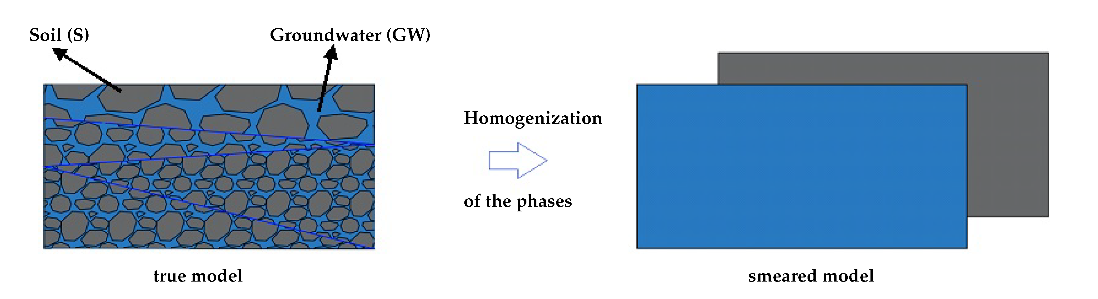
2.1. Theory of Porous Media (TPM)

The most common multiphase homogenization strategies are the Biot theory (BT) [31], the Theory of Mixtures (TM) [17], and the Theory of Porous Media (TPM) [13,14]. The motivation for the theory and the introduction of homogenized quantities are the primary differences between the models. While considering other mixture approaches, we employ the Theory of Porous Media because it provides a framework that is both robust and thermodynamically consistent. The authors have already been able to answer a number of various engineering questions using single-scale macroscopic homogenization approaches, such as in soil mechanics [19,20], material science [32], environmental engineering [33,34], or continuum biomechanics [35]. While considering other mixture approaches, we employ the Theory of Porous Media because it provides a framework that is both robust and thermodynamically consistent. Similarly to mixture theory, the constituents are distributed statistically over the control space, and the system is considered to be in ideal disorder. The mixture approach is coupled with the concept of volume fractions, in which the total of the volume fractions is considered to be equal to one. In contrast to the classical continuum-mechanical description of one-component continua, the Theory of Porous Media considers a mixture consisting of κ constituents φ α with α = 1 , , κ .

2.2. Extended Theory of Porous Media (eTPM)

The extended TPM (eTPM) provides an approach in case that the immiscible macroscopic phases are additionally composed of different substances. For example, groundwater can consist of an incompressible carrier phase and therein dissolved contaminants.

2.2.1. Immiscible Constituents

In the framework of the eTPM [36], it is assumed that all constituents of the overall aggregate are to be in a state of ideal disarrangement and defined by a local representative elementary volume (REV) [20]. The overall aggregate structure is then smeared over the REV by the prescription of a volumetric averaging process leading to a statistical substitution of the original microstructure, cf. Figure 1. Hence, all geometrical and physical quantities are defined as the statistical mean values of the occurring actual quantities. The smearing procedure over REV leads to the biphasic superimposed and interacting continua model, and the composition of the porous medium can be written as follows:
φ = α φ α = φ S φ GW ,
wherein φ refers to the multi-phase continuum porous medium and α { S , GW } denote its individual constituents, namely soil and groundwater. The definition of the volume fraction n α , cf. Equation (2) [15], for each phase at each point determines the local compositions of the aggregate with
n α = dv α dv .
Therein, dv α and dv indicate the local ratios of the partial volume elements and the volume element of the overall aggregate, respectively. As a consequence, the volume V of the overall aggregate and the partial volumes v α of the constituent α are given by
V = B S dv = α κ V α , V α = B S n α dv .
From Equation (3), the saturation condition can be written as follows:
α = 1 κ n α x , t = n S + n GW = 1 .
This needs to be satisfied to prevent the development of vacant space during possible deformation processes of the overall body B S . Based on the definition of the volume fraction for each phase, a partial density ρ α can be introduced by:
ρ α = dm α dv .
The real density ρ α R relates the local mass dm α to the volume element dv α , whereas the partial density ρ α relates the same mass to the volume element dv . The partial density can be concluded from Equation (3) and can be written as follows:
ρ α = n α ρ α R .

2.2.2. Miscible Concentration

Incorporating the transport of miscible components, namely contaminants, the framework of TPM needs an extension of TPM [20]. The composition of the porous medium according to the eTPM can be read as follows:
φ = α = 1 κ φ α = α = 1 κ φ α + β = 1 ν φ α β .
Since the volume fraction of immiscible phases, including miscible components, change minimally, therefore, the contribution of miscible contaminants in their carrier phase is considered by means of concentrations. Regarding this, the mixture molar concentration and the phase molar concentration of the contaminants can be read as follows:
c β = dn mol β dv , c α β = dn mol β dv α ,
wherein dn β = dm β / M mol β denotes the number of moles of a solute φ α β in a carrier phase φ α , dm β and M mol β are the molar mass and local mass of the miscible components φ α β , respectively. Analogous to immiscible phases, the partial and real density of the miscible contaminants can be defined as follows:
ρ α β R = dn mol β dv = c α β M mol β , ρ α β = dn mol β dv α = n α c α β M mol β .
Herein, α β denotes a contaminant in groundwater, namely GWC.

2.3. Field Equations and Constitutive Theory

A quasi-static, biphasic model with an incompressible solid phase and liquid phase, including contaminant under isothermal conditions, was developed. The set of coupled field equations, including the balance equations, namely balance of mass and momentum, and restrictions associated with the volume fractions and interaction forces, is required to calculate the unknown quantities. These equations can be read as follows [19,20]:
n S S + n S div x S = 0 , n GW S + n GW div x S + div n GW w GWS = 0 , n GW S c GWC + n GW c GWC S + div j GWC + n GW c GWC div x S = 0 , div T S + ρ S ( b ) = p ^ S , div T GW + ρ GW ( b ) = p ^ GW , div T GW C + ρ GW C ( b ) = p ^ GW C , n S S + n GW GW grad n GW w GWS = 0 , α = 1 κ p ^ α = p ^ S + p ^ GW = 0 , n S + n GW = 1 .
Herein, w GWS = x GW x S denotes the relative velocity. In addition to the kinematics and field equations, constitutive relations are required so as to complete the system of equations. These constitutive relations can be obtained by the evaluation of the mixture entropy inequality, which can be expressed as follows:
α = 1 κ ρ α ψ α α + ρ ^ α ψ α 1 2 x α · x α + T α · D α p ^ α · x α 0 ,
wherein ψ α = ϵ α θ η α denotes the Helmholtz free energy with the specific entropy η α and the internal energy ϵ α of φ α . The dependence of the Helmholtz free energies ψ α is reduced and limited in order to maintain the complication of a comprehensive assessment as follows:
ψ S = ψ S C S , ψ GW = ψ GW , ψ GWC = ψ GW C c GWC ,
wherein, ψ S , ψ GW , and ψ GWC are Helmholtz free energy functions for soil, groundwater and contaminant, respectively. C S and c GWC denote the right Cauchy–Green deformation tensor of soil and contaminant concentration.

2.4. Evaluation of the Entropy Inequality

The non-isothermal process such as the transport of the contaminant in the groundwater through the soil in the framework of the eTPM can depend on the temperature, volume fraction, density, deformation, actual velocity, and their appropriate gradients as follows:
V = { θ α , grad θ α , n α , grad n α , ρ α , grad ρ α , F α , Grad α F α , x ´ α , Grad α x ´ α , X α , c GWC } .
The temperature θ α describes the thermal state of each constituent φ α . The volume fraction n α , real density ρ α R and deformation gradient F α , as well as their gradients, define the deformation of the constituents. x ´ α and Grad α x ´ α have been utilized in order to describe the viscosity effect. The initial position X α is required in order to describe the inhomogeneous material behaviour. The following set of undetermined response functions R , which cannot be determined from the balance equations with the knowledge of the full state of motion, can be read as
R = { ψ S , ψ GW , ψ GWC , T S , T GW , T GWC , p ^ GW , p ^ GWC } ,
wherein, T S , T GW , T GWC denote the Cauchy stress tensor for soil, groundwater and contaminant, respectively. p ^ GW , p ^ GWC are the direct momentum production of the groundwater and contaminant. Since there is no mass exchange between soil and groundwater and the real density of the soil is constant, the mass balance of the soil can be reduced as follows:
( n S ) S + n S div x S = 0 ,
and the actual solid volume fraction can be read as
n S = n 0 S S ( det F S ) 1 ,
where n 0 S S denotes the initial volume fraction of the soil. Utilizing the saturation condition, which means there is any vacant space in the porous body [15], the volume fraction of the fluid can be read as
n GW = 1 n 0 S S ( det F S ) 1 .
Consequently, the volume fraction of phases and their respective gradients can be eliminated from the set of independent process variables. Furthermore, assuming the same temperature for both phases, the temperature and its gradient were eliminated from the process variables. Based on the material frame indifference (material objectivity), which indicates that a physical phenomenon should not depend on the position of observation, the velocity x α and its respective gradient Grad α x α are replaced by the material frame independent seepage velocity and the symmetric parts of the velocity gradients, respectively. Furthermore, the deformation gradient F S has to be replaced by the right Cauchy-Green deformation tensor C S since F S is also frame-dependent. Consequently, in order to describe the contaminant transport in groundwater through the soil, the set of process variables is reduced to
S = { C S , Grad S C S , w GWS , D GW , c GWC } .

2.5. Adaption of the Entropy Inequality

In order to consider the restrictions from the saturation condition within the thermodynamical process, the Clausius-Planck inequality has to be enriched by the time derivative of this condition with respect to the solid deformation, which multiplies with a Lagrange multiplier λ as follows [33,37]:
λ n S + n GW S = 0 .
From the the mass balances for the soil φ S and groundwater φ GW , the time derivatives of their volume fractions can be read as
( n S ) S = n S D S · I , ( n GW ) GW = n GW D GW · I .
Considering the relation
( · ) L = ( · ) S + grad ( · ) · w GWS ,
Equation (10) can be rewritten as
λ n S D S · I + n GW D GW · I + grad ( n GW ) · w GWS = 0 .
The seepage velocity w GWS mainly depends on the permeability k D , which is assumed to be isotropic in the model formulation. However, utilizing a random field model enables to consider representatively anisotropic properties regarding permeability, cf. Random field method. The second adaptation is accomplished by inserting another Lagrange multiplier λ GWC for the balance of mass of the contaminant, which enlarges the entropy inequality. This multiplier can be introduced as follows:
λ GWC c GWC D GW · I + λ GWC n GW c GWC GWC + λ GWC c GWC grad n GW · w GWCGW + λ GWC n GW c GWC D GWC · I = 0 .
Conclusively, the modified entropy inequality reads
D S · { T S 2 ρ S F S ψ S C S F S T + n S λ I } + D GW · { T GW + n GW λ I + n GW c GWC λ GWC I } + D GWC · { T GWC + n GW c GWC λ GWC I } + c GWC GWC { ρ GWC ψ GWC c GWC λ GWC n GW } + D is 0 ,
with the dissipation mechanism
+ D is = w GWS · { p ^ GW + λ grad n GW λ GWC c GWC grad n GW } w GWCS · { p ^ GWC + λ GWC c GWC grad n GW } 0 .
It is necessary to set the energy-preserving factors to zero in order to satisfy the entropy inequality since they are conservative and do not increase the entropy of the system. Following this, the constitutive relations for stresses and pressures, which act on the phases and the contaminant, can be obtained:
T S = 2 ρ S F S ψ S C S F S T n S λ I , T GW = n GW λ I + T GWC , T GWC = n GW c GWC λ GWC I
with
λ GWC = ρ GWC n L c mol GWC ψ GWC c mol GWC ,
λ can be translated as the reaction force between the solid and fluid phase identifying the pore pressure [15]. Since the stress of the liquid is dominated by the effective pore water pressure and T GWC is neglected. The evaluation of the dissipative terms of the entropy inequality yields the following momentum production terms for the soil, water phase and the contaminant with
p ^ GW = λ grad n GW I λ GWC c GWC grad n GW I α wGWS w GWS + α wGWCS w GWCS , p ^ GWC = λ GWC c GWC grad n GW I α wGWS w GWS α wGWCS w GWCS .
The factors α wGWCS and α wGWS , which are material parameters, are restricted to a positive value.

2.6. The Chemical Potential as a Free Helmholz Energy Function for a Contaminant

The chemical potential μ is a useful quantity that is indispensable not only in chemistry but also in physics, such as for the Helmholtz free energy function for a contaminant as a miscible constituent. Furthermore, it is crucial for the understanding of many processes dealt with in physics. Moreover, the chemical potential can reveal the direction in which a phase transition proceeds. Also, the pressure and temperature dependence of a phase transition can be calculated via the chemical potential. It is also needed for the description of equilibria in which two driving forces compensate for each other. The chemical potential for a constituent within a mixture can be defined as the gradient of the free energy of the system with respect to a change in the number of moles of the constituent [19,20,37]. Accordingly, with respect to the miscible constituents considered here, the chemical potential is defined as [38]
μ α β = R θ ln c α β c 0 α β + μ 0 α β ,
wherein R [ J / ( mol K ) ] is the universal gas constant, θ [ K ] , c 0 α β and μ 0 α β denote the absolute temperature, the reference concentration, and reference chemical potential, respectively. The energy function for the solutes φ α β is given as a volume-specific energy such that
ψ α β = 1 M mol β c α β { R θ ln c α β c 0 α β + 1 + μ 0 α β } .

2.7. Stresses and Interaction Forces

In the following, the Helmholtz free energy functions for soil and contaminant are assumed:
ψ S = 1 ρ 0 S R 1 2 λ S ln J S 2 μ S ln J S + 1 2 μ S tr C C S 3 , ψ GWC = 1 M mol C c GWC { R θ ln c GWC c GWC 0 + 1 + μ 0 GWC } ,
wherein λ S and μ S denote Lamé constants, R indicates the general gas constant, θ is indicative of the absolute temperature of the mixture, μ 0 GWC and c 0 GWC are representative of reference chemical potential and reference concentration, respectively. The outcome of these assumptions are the following stress relations:
T S = 1 J S λ S ln J S I + μ S K S n S λ I , T GW = n GW λ I + T GWC , T GWC = n GW μ GWC I .

2.8. Numerical Treatment

Using standard Galerkin finite element method, the weak formulations of the local balance equations are developed [19,20,37]. The weak counterparts of the strong local form of the mechanical balance equations are developed by integration and multiplication of the strong form with the following independent weighting functions:
W = { δ u S , δ p GWR , μ GWC } .
Having weighted and applied the product rule and the Gaussian integral theorem, the weak forms of the momentum balance equations are read as follows:
  • Balance of momentum for the mixture
B S α S , GW , GWC T α · grad δ u S d v B S α S , GW , GWC ρ α b · δ u S d v = B S t · δ u S d a .
  • Balance of mass for the mixture
B S n GW w GWS · grad δ p GWR d v B S n GW S + n GW tr D S δ p GWR d v = B S n GW w GWS · n δ p GWR d a .
  • Balance of mass for the contaminant
B S n GW c GWC S δ μ GWC d v B S j GWC · grad δ μ GWC d v + B S n GW C GWC tr D S δ μ GWC d v = B S j GWC · n δ μ GWC d a .

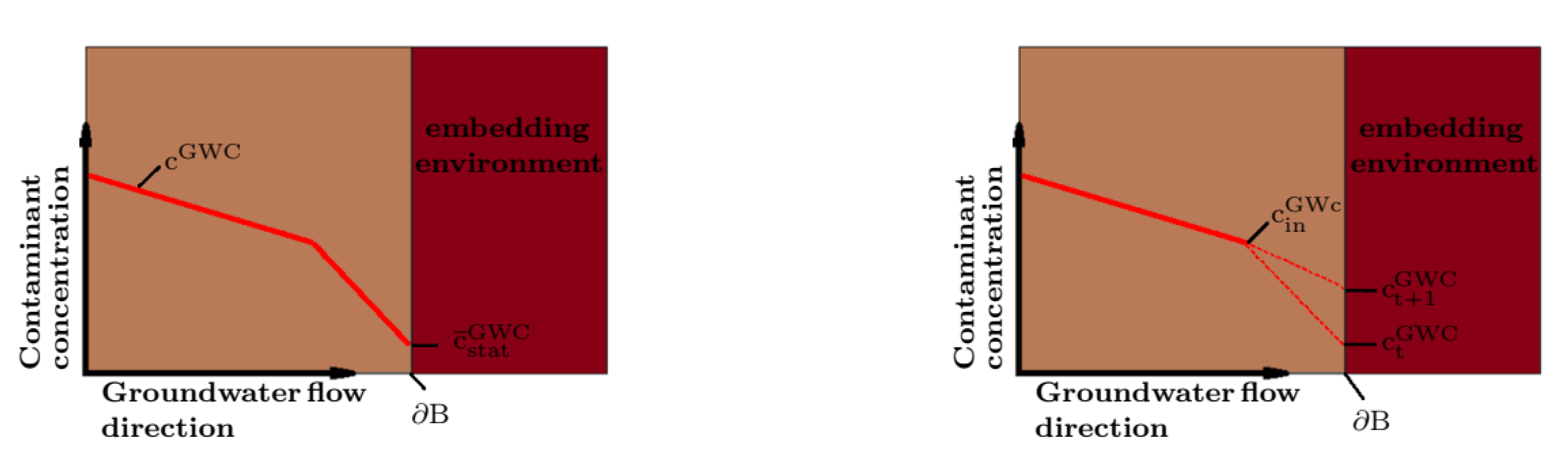
2.9. Stabilized Boundary Conditions for Contaminant Transport

In this section, the contaminant flux out of the given system has been addressed. The major issue in this regard is the correspondence between the boundary conditions for the contaminant and the flux of the contaminant carrying groundwater. At the considered geometry boundaries, cf. Figure 2, representing a flux for the groundwater, the contaminant flux should correspond to the efflux of groundwater carrying the contaminants. By defining static boundary conditions for the contaminant numerically at the flux boundary, an erroneous gradient of the respective contaminant is achieved through the fluent boundary elements. This issue exists both for, Dirichlet boundary conditions, where the solute concentration should be prescribed, and Neumann boundary conditions, where the contaminant concentration flux should be determined. By this erroneous gradient that manifests only within finite elements placed right at the boundary, instabilities of the FE simulation and disturbances of the contaminant transport simulation are obtained. Hence, an updating algorithm is required for the contaminant boundary conditions to approximate the solute boundary condition. Initiating from the initial or static boundary value, the dynamic boundary value is updated by the considered explicit Euler algorithm at the finite element nodes on the Dirichlet boundary followed during each time period by an expected difference in the boundary values. Owing to the explicit Euler approximation, the boundary value is oriented by the solution from the actual time period as follows:
c ¯ t + 1 GWC = c ¯ t GWC + Δ c ¯ GWc , Δ c ¯ GWC ( c in GWC , c ¯ t GWC ) ,
wherein c in GWc represents the contaminant concentration at the FE nodes of the boundary element opposite to the outflow boundary. By selecting Δ c ¯ GWc = ( c GWc c ¯ t GWc ) / 2 , an adequate stabilization is indicated for the erroneous gradient with a smooth gradient within the elements ahead of the outflow boundary [39,40].

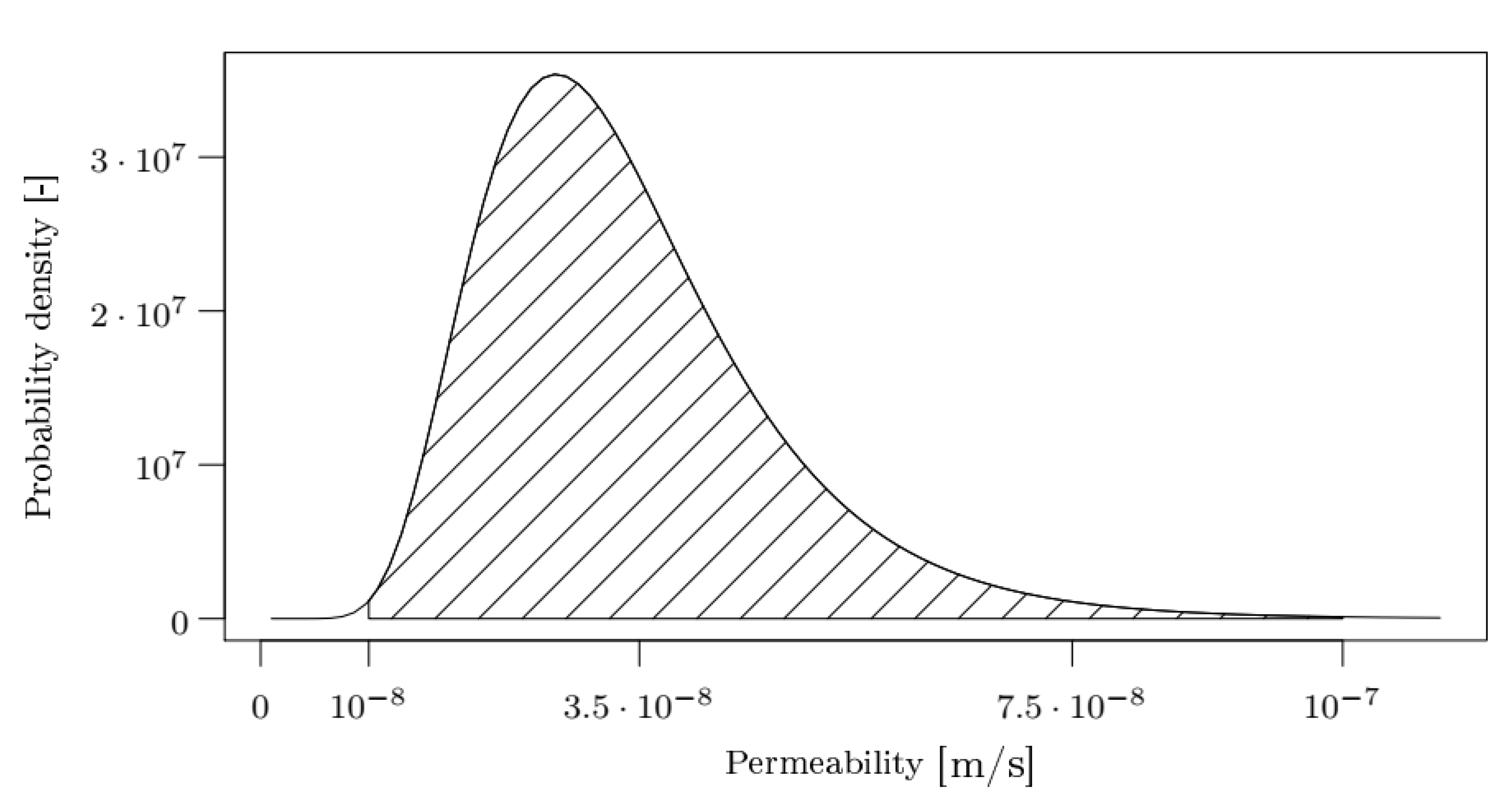
2.10. Random Field Method

It is assumed that a soil layer property (e.g., permeability) typically has values in the interval a , b with a < b . Instead of presuming that the values of this property are equal in each point x of the layer the values are assumed as realizations of a Log-Gaussian random field. A random field is a family of random variables at locations x D  [41].
Z x | x D R d , d 1
If the distribution of the random vector Z = Z x 1 , , Z x n T is multivariate Gaussian for arbitrary locations x 1 , , x n , the field is called a Gaussian random field. Hence, this field can be fully characterized through the expectation μ ˘ x = E Z x and the covariance function κ ˘ x , x = C o v Z x , Z x with x , x D . In the following, consider a Gaussian random field with constant expectation μ ˘ x = μ ˘ x D and the covariance function
κ ˘ x , x = σ ˘ 2 ρ ˘ x x , Ψ x , x D
that only depends on the constant process variance σ ˘ 2 and the correlation function ρ ˘ . The correlation function determines the dependency structure of the random field values through the distance between the points.
A well known correlation function is the exponential correlation function
ρ ˘ x x , Ψ = exp x x Ψ
with a single-scale parameter Ψ and where x x denotes the Euklidian distance between x and x . Figure 3 shows how the scale parameter affects the correlation of two random field variables Z x and Z x depending on their distance x x . For small values of Ψ , the correlation converges very fast to zero. Hence, variables with a distance greater than 5 are almost uncorrelated for Ψ = 1 . For higher values than Ψ = 8 , the correlation function converges much slower, but the moderate and high correlation only occurs between variables located within a distance of 8 or smaller. For the random field model of permeability values, a scale of 8 is chosen to prevent sudden value changes in the random field realizations. To achieve that, the realized values z are in the provided interval a , b , the mean is determined as
μ ^ = 1 2 log a + log b
and the standard deviation is determined as
σ ^ = 1 k μ ^ log a
with k N . For k = 3 (as chosen here), the realized values z of a Gaussian distribution with expectation μ ^ and standard deviation σ ^ are included in the interval μ ^ 3 σ ^ , μ ^ + 3 σ ^ = log a , log b with a probability of 0.99 . Hence, the values of the permeability z = exp z are in a , b with the same probability (cf. Figure 4).
Thus, to obtain the permeability values for n locations of a single layer, a Gaussian random field with the input parameters scale ψ = 8 , mean μ = μ ^ and variance σ 2 = σ ^ 2 is realized on the logarithmized value interval log a , log b and the resulting values z 1 , , z n are transformed as z 1 = exp z 1 , , z n = exp z n in order to come back to the original scale with the interval a , b . The calculations are performed using the statistical open source software R with the package RandomFields [42]. For the soil model with three layers, the Gaussian random field parameters are listed in Table 1.

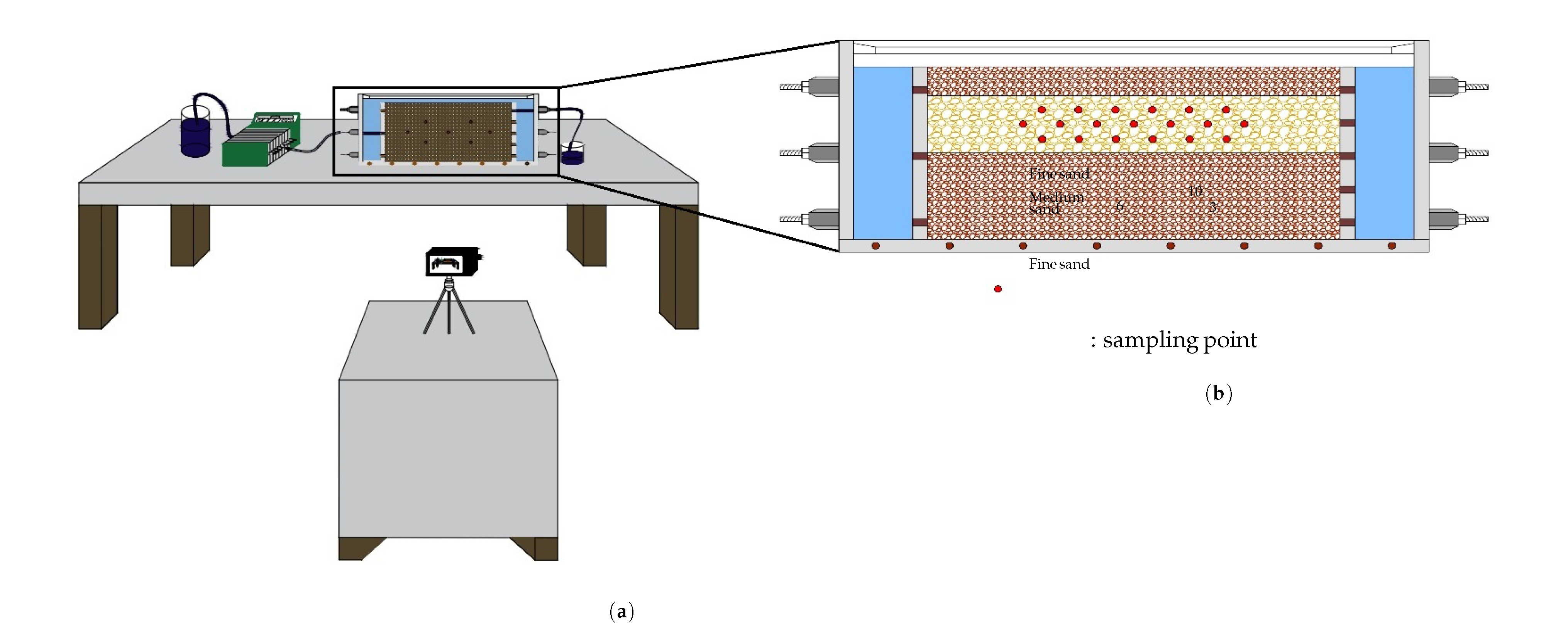
2.11. Physical Sandbox Experiment

The schematic of the physical sandbox experiment is illustrated in Figure 5. The experiment was conducted in a plexiglass tank [1.5 × 0.38 × 0.10 m]. At each end of the sandbox are constant head tanks which are separated from the rest of the box by one impermeable wall and one perforated mesh filter to keep the sand out of the head tanks. Three different layers of sand were added to the tank (Figure 5). The bottom layer [15 cm] is low permeable sand (3.6 × 10 6 m/s), the middle layer [12 cm] is high-permeability sand 2.75 × 10 4 m/s) and the top layer [8 cm] is low-permeability sand (3.6 × 10 6 m/s). The sand was compacted according to our earlier work [2,43]. During the compaction, the fine sand was saturated in order to achieve proper compaction and avoid any leakage of the tracer. A peristaltic pump (Watson Marlow) was used for circulating water in the system. The pump can deliver a maximum of 41 [L/h]. The characteristics of the two different sizes of sand, are given in Table 2. Hydraulic conductivity was measured by using the constant-head method [39,44]. The tank was pre-flushed to remove fines, and a continuous flow state was established for two hours through a peristaltic pump. After the saturation of all the layers, the injection of the tracer (potassium permanganate) was initiated by supplying 15 [L] with a rate of 268 [mL/min] from the tank inlet. The flow of the tracer was taken into account after the injection in order to maintain the same steady-state flow of the pre-flushed stage. The key properties of potassium permanganate in this study are the extensive use in the water treatment industry and the intensely purple color that permits the visual observation of the distribution during the entire process. The tracer was released through a 9 [cm] line source of a 3 [mm] diameter tube located in the middle, high permeability sand layer. Upon release through the line source at the middle layer, the tracer was expected to preferentially migrate through the more permeable medium sand, with the fine sand ensuring tracer containment within the middle layer. The experiment was successfully completed when all permeable layers were fully saturated by the tracer. The monitoring of the tracer was accomplished by photo shoots and the measurement of total dissolved solids (TDS) using a conductivity meter at observation points within the tank to calculate permanganate concentration during the progress of the experiment (Figure 5).

2.12. Field Scale Simulation

The assessment of the effectiveness of the combined eTPM and Random Fields to quantify the understanding of the effect of permeability on the contaminant transport required the analysis of the plume distribution in heterogenous systems. The purpose of our numerical study is to understand the effect of permeability heterogeneity on the contaminant fate. A multi-layer contaminant transport scenario with varying permeabilities is simulated, similar to what could be expected with rapidly changing shallow alluvial sediments. The aquifer domain is made of rectangles with dimensions of 2000 [m] by 100 [m] , which are heterogeneous regarding permeability, cf. Figure 5. The simulation was performed for 300 days, with a time step of 0.001 days . The simulation has been repeated for 500 different realizations of permeability in the aquifer domain. The initial contaminant concentration is c 0 = 10 [mg/L] on the left-hand side of the aquifer.

3. Results and Discussion

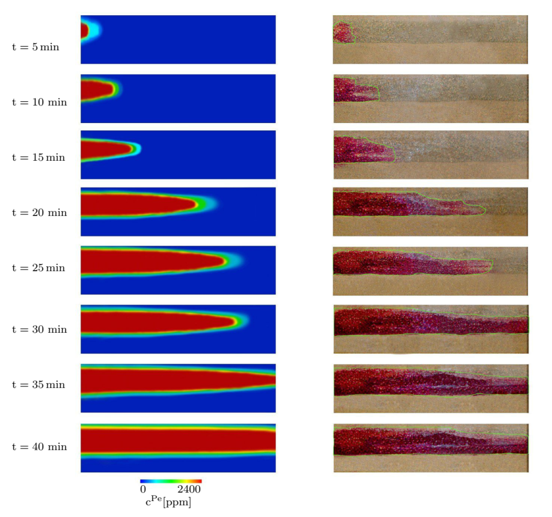
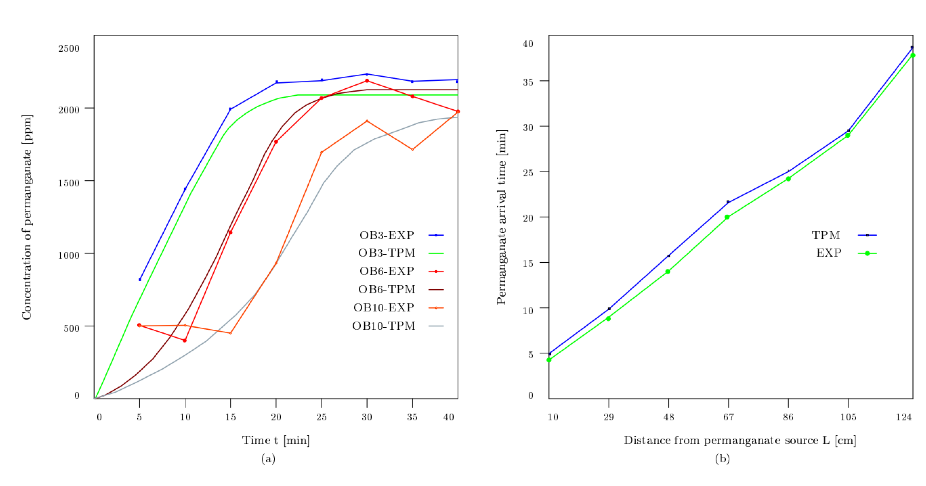
3.1. Validation with the Physical Sandbox Experiment

Table 3 compared parameters between simulation and physical sandbox experiment.
Figure 6 represents the comparison between numerical and experimental results in terms of the permanganate plume distribution in a 3-layer aquifer system of varying permeability. As can be seen in the Figure 6, the simulation closely matches the experiment except that in the simulation, the interface is blurred because of numerical dispersion, which was to minimize by a fine mesh discretization. This matching indicates the effectiveness of the eTPM approach. To compare the measured permanganate concentration in the physical sandbox test and the eTPM approach, 19 sampling points have been considered in the middle layer of the soil, cf. Figure 5. Figure 7 compares the measured permanganate concentration and eTPM simulation for the explained three sampling points (in [cm]), P 6 (19.5,18), P 3 (78,18) and P 10 (67,21) with respect to the origin, which is located at the bottom corner of the input end of the tank. The total dissolved solids (TDS) were measured for the calculation of permanganate concentration every 5 min after injection. The average absolute difference between measured and predicted concentrations is 5.21%. The mean square error (MSE) equals 78 ppm. The percentage difference between the measured and predicted concentrations shows that the results are in good agreement with the maximum percentage error between experimental and numerical models of 12.3% at one sampling point. In general, the measured and predicted contaminant concentrations were in good agreement in all observation points at different times. The differences at some time steps can be explained by the movement of the mass, the compression in specific points, and the dilution effect caused by the hydrodynamic dispersivity being smaller on this scale than in real conditions.
Figure 7 compares the measured and predicted arrival time of the permanganate. The average absolute difference between experimental and numerical results equals 7.21%. The mean square error equals 6.5 min.

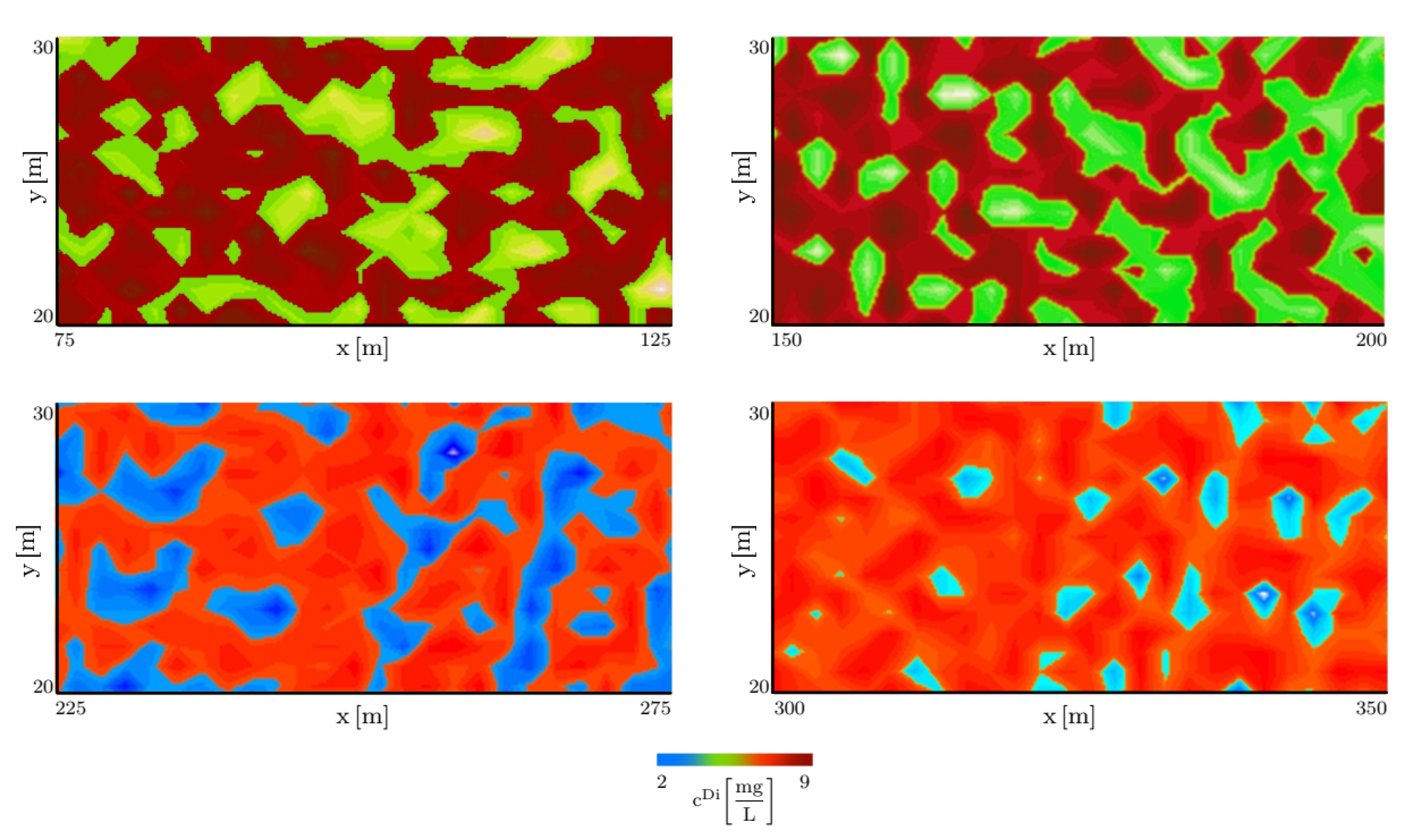
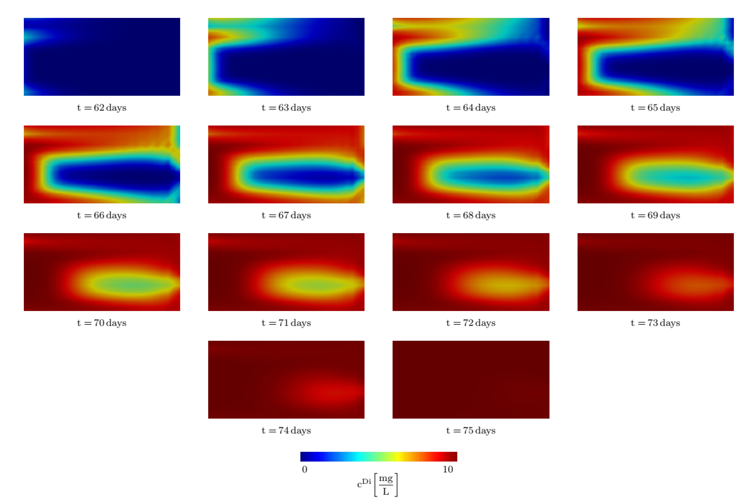
3.2. Transport of Contaminant in Groundwater through Three-Layer Heterogeneous Alluvial System

Figure 8 is a field scale example of permeability as a realization of the three Log-Gaussian random fields for the three layers of differing permeability in a shallow alluvial aquifer. Such systems such as river terrace gravels can show high heterogeneity of permeability over small distances. The output is an example of a model subsection measuring 100 m long and 50 m deep with the deepest layer 1 having permeabilities ranging from 2 × 10 7 [ m / s ] to 6 × 10 7 [ m / s ] (low permeability zone); layer 2 having permeabilities ranging from 2 × 10 6 to 8 × 10 6 [ m / s ] (high permeability zone); and the shallowest layer 3 having permeabilities ranging from 2 × 10 8 to 1 × 10 7 [ m / s ] (lowest permeability zone). This random field realization of permeability when coupled with the eTPM contaminant transport gives very different output when compared with a modelled homogenous 3-layer aquifer permeability . Figure 9 presents the concentration color map of the considered geometry, which is located (in [m]) between (75,20) and (125,30), (150,20) and (200,30), (225,20) and (275,30), and (300,20) and (350,30) after 128 days for one realization of permeability shown in Figure 8.
In the homogeneous situation, the plume must conform to an idealized wedge-like shape; however, in the heterogeneous state, the plume is completely deformed. Yet, when the contaminant flows over the low heterogeneous permeable zone, there is no corresponding distortion of the wedge in the overall geometry of the system. This Anisotropy or spatial correlation in the permeability distribution results in different concentration thresholds along the x- or y-axis and, consequently, shifts in the quantities such as seepage velocity. Figure 10 demonstrates the contaminant concentration distribution for the area between (85,21) and (90,25) for different times indicating the random field’s good performance in the small-scale case. Because the system’s preferred groundwater paths are blocked by zones of low permeability caused by spatially heterogeneous permeability, the importance of viscous dissipation effects can increase.
Figure 11 demonsrates the histogram of the average contaminant concentration at t = 100 days and the arrival time of the contaminant in this area calculated for 500 realizations for permeability. The contaminant arrival time could be affected strongly by random realizations. The breakthrough time is generally shorter than the homogeneous condition. Using the 75% confidence interval (CI), the average contaminant concentration shows 4.4% variation from the average values the considered area and 8.9% in the case of a 95% confidence interval. Utilizing the 95% confidence interval, the contaminant arrival time indicates 7.2% from average arrival time.
From an engineering perspective, random fields (RFs) are an appropriate method for capturing the effects of soil-specific uncertainty on numerical models [18,27,45]. This study demonstrates the compatibility of both methods with regard to numerical stability of the multiphase model as well as manageability of their respective requirements. The method provides significant information as a decision-making tool for end-users, who can, e.g., formulate more precise requirements for site investigations and scientific purposes. A major advantage is that the information is available with just one single run of the simulation and the universal applicability of the method. Another advantage is the accurate approximation of the solution space and the efficient computation time. The disadvantage of the model lies in algorithmic implementation.

4. Conclusions

It is challenging to develop a realistic numerical groundwater model to represent a site condition with complex geological conditions such as variation in permeability. This paper focuses on the impact of the permeability distribution on contaminant transport, as it is the significant parameter controlling contaminant transport after hydraulic gradient. Here, the combined Random Field eTPM numerical model has been verified with a physical sandbox experiment. The simulation has been performed on a rectangular geometry, consistent with a non-unidirectional permeability gradient along x- or y-axis, the model can be used for a real-world example of a heterogeneous contaminated scenario e.g., contaminant flow in river terrace or alluvial gravels. The simulation results are in good agreement with the experimental results, in which the maximum percentage difference between measured and predicted concentration is less than 12%. In our previous study, the contaminant transport was modeled on the basis of two different approaches, namely, eTPM and CFD. The contaminant concentration at two points of the the microfluidic chip was compared with the numerical results. Although there was no significant difference between the measured contaminant concentration and the predicted one, eTPM was in better agreement with the experiment [20]. The combined eTPM and random field method to investigate the effect of permeability on the contaminant transport allowed the interpretation of essential characteristics and changes in the contaminant concentration and arrival time. This novel numerical approach has demonstrated itself a valuable tool to reduce uncertainty associated with contaminant transport in heterogenous porous media. This approach can enhance the presented model, including a macroscale and a microscale. Furthermore, the chemical reactions between soil and contaminant and oxidant and contaminant can be considered. The primary limitation of the three-layer experimental setup is that it does not facilitate a physical sandbox aquifer with high-resolution hydraulic tomography characterization.

Author Contributions

Study concept and design: S.M.S., R.D., T.R. Physical tank test experiment: S.M.S., P.K. TPM SimulationIn and plementation of the model in FEAP: S.M.S., C.H. Random field simulation of permeability: S.M.S., C.H., S.H., K.I. Analysis of data: S.M.S. Interpretation of data: S.M.S. Writing manuscript: S.M.S. Critical revision: All authors. All authors have read and agreed to the published version of the manuscript.

Funding

This work was completed as part of the REMEDIATE (Improved decision-making in contaminated land site investigation and risk assessment) Marie-Curie Innovation Training Network. The network has received funding from the European Union’s Horizon 2020 Programme for research, technological development and demonstration under grant agreement n. 643087. REMEDIATE is coordinated by the QUESTOR Centre at Queen’s University Belfast.

Conflicts of Interest

The authors declare no conflict of interest.

Abbreviations

The following abbreviations are used in this manuscript:
BaREBayesian recursive estimation
CIconfidence interval
eTPMextended Theory of Porous Media
GLUEGeneralized likelihood uncertainty estimation
MCMCMarkov chain Monte Carlo
MSEmean square error
RFrandom fields
REVrepresentative elementary volume
TPMTheory of Porous Media
TDStotal dissolved solids

References

  1. Patil, S.; Chore, H. Contaminant transport through porous media: An overview of experimental and numerical studies. Adv. Environ. Res. 2014, 3, 45–69. [Google Scholar] [CrossRef] [Green Version]
  2. Seyedpour, S.; Kirmizakis, P.; Brennan, P.; Doherty, R.; Ricken, T. Optimal remediation design and simulation of groundwater flow coupled to contaminant transport using genetic algorithm and radial point collocation method (RPCM). Sci. Total. Environ. 2019, 669, 389–399. [Google Scholar] [CrossRef] [Green Version]
  3. Rosén, L.; Back, P.E.; Söderqvist, T.; Norrman, J.; Brinkhoff, P.; Norberg, T.; Volchko, Y.; Norin, M.; Bergknut, M.; Döberl, G. SCORE: A novel multi-criteria decision analysis approach to assessing the sustainability of contaminated land remediation. Sci. Total. Environ. 2015, 511, 621–638. [Google Scholar] [CrossRef]
  4. Wu, J.; Zeng, X. Review of the uncertainty analysis of groundwater numerical simulation. Chin. Sci. Bull. 2013, 58, 3044–3052. [Google Scholar] [CrossRef] [Green Version]
  5. Zadeh, L.A. Toward a generalized theory of uncertainty (GTU)—An outline. Inf. Sci. 2005, 172, 1–40. [Google Scholar] [CrossRef]
  6. Liu, P.; Shu, L. Uncertainty on numerical simulation of groundwater flow in the riverside well field. J. Jilin Univ. (Earth Sci. Ed.) 2008, 38, 639–643. [Google Scholar]
  7. Merz, B.; Thieken, A.H. Flood risk curves and uncertainty bounds. Nat. Hazards 2009, 51, 437–458. [Google Scholar] [CrossRef] [Green Version]
  8. Yang, P.; Yuan, D.; Yuan, W.; Kuang, Y.; Jia, P.; He, Q. Formations of groundwater hydrogeochemistry in a karst system during storm events as revealed by PCA. Chin. Sci. Bull. 2010, 55, 1412–1422. [Google Scholar] [CrossRef]
  9. Singh, A.; Mishra, S.; Ruskauff, G. Model averaging techniques for quantifying conceptual model uncertainty. Groundwater 2010, 48, 701–715. [Google Scholar] [CrossRef]
  10. Fiori, A.; Zarlenga, A.; Bellin, A.; Cvetkovic, V.; Dagan, G. Groundwater contaminant transport: Prediction under uncertainty, with application to the MADE transport experiment. Front. Environ. Sci. 2019, 7, 1–15. [Google Scholar] [CrossRef] [Green Version]
  11. Prasad, K.L.; Rastogi, A. Estimating net aquifer recharge and zonal hydraulic conductivity values for Mahi Right Bank Canal project area, India by genetic algorithm. J. Hydrol. 2001, 243, 149–161. [Google Scholar] [CrossRef]
  12. Ehlers, W. Poröse Medien: Ein Kontinuumsmechanisches Modell auf der Basis der Mischungstheorie; Universität-GH Essen: Duisburg, Germany, 1989. [Google Scholar]
  13. Ehlers, W. Foundations of multiphasic and porous materials. In Porous Media; Springer: Berlin/Heidelberg, Germany, 2002; pp. 3–86. [Google Scholar]
  14. De Boer, R. Theory of Porous Media: Highlights in the Historical Development and Current State; Springer: Berlin/Heidelberg, Germany, 2000. [Google Scholar]
  15. Ehlers, W.; Bluhm, J. Porous Media: Theory, Experiments and Numerical Applications; Springer Science & Business Media: Berlin/Heidelberg, Germany, 2013. [Google Scholar]
  16. Ricken, T.; Schröder, J.; Bluhm, J.; Maike, S.; Bartel, F. Theoretical formulation and computational aspects of a two-scale homogenization scheme combining the TPM and FE2 method for poro-elastic fluid-saturated porous media. Int. J. Solids Struct. 2022, 241, 111412. [Google Scholar] [CrossRef]
  17. Bowen, R. Toward a thermodynamics and mechanics of mixtures. Arch. Ration. Mech. Anal. 1967, 24, 370–403. [Google Scholar] [CrossRef]
  18. Schmidt, A.; Henning, C.; Herbrandt, S.; Könke, C.; Ickstadt, K.; Ricken, T.; Lahmer, T. Numerical studies of earth structure assessment via the theory of porous media using fuzzy probability based random field material descriptions. GAMM-Mitteilungen 2019, 42, 1–15. [Google Scholar] [CrossRef] [Green Version]
  19. Seyedpour, S.M.; Ricken, T. Modeling of contaminant migration in groundwater: A continuum mechanical approach using in the theory of porous media. PAMM 2016, 16, 487–488. [Google Scholar] [CrossRef]
  20. Seyedpour, S.; Janmaleki, M.; Henning, C.; Sanati-Nezhad, A.; Ricken, T. Contaminant transport in soil: A comparison of the Theory of Porous Media approach with the microfluidic visualisation. Sci. Total. Environ. 2019, 686, 1272–1281. [Google Scholar] [CrossRef]
  21. Huggi, V.; Rastogi, A. Estimation of solute transport parameters of groundwater systems using genetic algorithm. Water Energy Int. 2003, 60, 38–45. [Google Scholar]
  22. Hassan, A.E.; Bekhit, H.M.; Chapman, J.B. Uncertainty assessment of a stochastic groundwater flow model using GLUE analysis. J. Hydrol. 2008, 362, 89–109. [Google Scholar] [CrossRef]
  23. Tsai, F.T.; Li, X. Inverse groundwater modeling for hydraulic conductivity estimation using Bayesian model averaging and variance window. Water Resour. Res. 2008, 44, 1–15. [Google Scholar] [CrossRef]
  24. Rackwitz, R. Reviewing probabilistic soils modelling. Comput. Geotech. 2000, 26, 199–223. [Google Scholar] [CrossRef]
  25. Geyer, S.; Papaioannou, I.; Graham-Brady, L.; Straub, D. The spatial averaging method for non-homogeneous random fields with application to reliability analysis. Eng. Struct. 2022, 253, 1–14. [Google Scholar] [CrossRef]
  26. Vanmarcke, E.H. Probabilistic modeling of soil profiles. J. Geotech. Eng. Div. 1977, 103, 1227–1246. [Google Scholar] [CrossRef]
  27. Henning, C.; Ricken, T. Polymorphic uncertainty quantification for stability analysis of fluid saturated soil and earth structures. PAMM 2017, 17, 59–62. [Google Scholar] [CrossRef] [Green Version]
  28. Henning, C.; Herbrandt, S.; Ickstadt, K.; Ricken, T. Combining Finite Elements and Random Fields to Quantify Uncertainty in a Multi-phase Structural Analysis. PAMM 2018, 18, 1–4. [Google Scholar] [CrossRef]
  29. Fiori, A. On the influence of local dispersion in solute transport through formations with evolving scales of heterogeneity. Water Resour. Res. 2001, 37, 235–242. [Google Scholar] [CrossRef]
  30. Suciu, N. Spatially inhomogeneous transition probabilities as memory effects for diffusion in statistically homogeneous random velocity fields. Phys. Rev. E 2010, 81, 1–8. [Google Scholar] [CrossRef]
  31. Biot, M.A. General theory of three-dimensional consolidation. J. Appl. Phys. 1941, 12, 155–164. [Google Scholar] [CrossRef]
  32. Ricken, T.; Bluhm, J. Evolutional growth and remodeling in multiphase living tissue. Comput. Mater. Sci. 2009, 45, 806–811. [Google Scholar] [CrossRef]
  33. Ricken, T.; Sindern, A.; Bluhm, J.; Widmann, R.; Denecke, M.; Gehrke, T.; Schmidt, T.C. Concentration driven phase transitions in multiphase porous media with application to methane oxidation in landfill cover layers. ZAMM-J. Appl. Math. Mech. Angew. Math. Mech. 2014, 94, 609–622. [Google Scholar] [CrossRef]
  34. Ricken, T.; Thom, A.; Gehrke, T.; Denecke, M.; Widmann, R.; Schulte, M.; Schmidt, T.C. Biological Driven Phase Transitions in Fully or Partly Saturated Porous Media. In Views on Microstructures in Granular Materials; Springer: Berlin/Heidelberg, Germany, 2020; pp. 157–183. [Google Scholar]
  35. Ricken, T.; Dahmen, U.; Dirsch, O. A biphasic model for sinusoidal liver perfusion remodeling after outflow obstruction. Biomech. Model. Mechanobiol. 2010, 9, 435–450. [Google Scholar] [CrossRef]
  36. Thom, A.; Ricken, T. In Silico Modeling of Coupled Physical-Biogeochemical (P-BGC) Processes in Antarctic Sea Ice. PAMM 2021, 20, 1–3. [Google Scholar] [CrossRef]
  37. Ricken, T.; Werner, D.; Holzhütter, H.; König, M.; Dahmen, U.; Dirsch, O. Modeling function–perfusion behavior in liver lobules including tissue, blood, glucose, lactate and glycogen by use of a coupled two-scale PDE–ODE approach. Biomech. Model. Mechanobiol. 2015, 14, 515–536. [Google Scholar] [CrossRef] [PubMed]
  38. Job, G.; Herrmann, F. Chemical potential—A quantity in search of recognition. Eur. J. Phys. 2006, 27, 353–371. [Google Scholar] [CrossRef] [Green Version]
  39. Seyedpour, S. Simulation of Contaminant Transport in Groundwater: From Pore-Scale to Large-Scale; Shaker Verlag: Herzogenrath, Germany, 2021. [Google Scholar]
  40. Werner, D. Two Scale Multi-Component and Multi-Phase Model for the Numerical Simulation of Biological Growth Processes in Saturated Porous Medi—At the Example of Fatty Liver in Human; Shaker Verlag: Herzogenrath, Germany, 2017. [Google Scholar]
  41. Vanmarcke, E. Random Fields: Analysis and Synthesis; World Scientific: Singapore, 2010. [Google Scholar]
  42. Schlather, M.; Malinowski, A.; Oesting, M.; Boecker, D.; Strokorb, K.; Engelke, S.; Martini, J.; Ballani, F.; Moreva, O.; Menck, P.J.; et al. Random-Fields: Simulation and Analysis of Random Fields. R package version 3.1.4. 2015.
  43. Seyedpour, S.; Valizadeh, I.; Kirmizakis, P.; Doherty, R.; Ricken, T. Optimization of the Groundwater Remediation Process Using a Coupled Genetic Algorithm-Finite Difference Method. Water 2021, 13, 1–18. [Google Scholar] [CrossRef]
  44. Sreekanth, J.; Datta, B. Comparing hydraulic conductivity through both inverted auger hole and constant head methods. Water Resour. Manag. 2014, 28, 1573–1650. [Google Scholar]
  45. Henning, C.; Ricken, T. Polymorphic Uncertainty Quantification of Computational Soil and Earth Structure Simulations via the Variational Sensitivity Analysis. PAMM 2019, 19, 1–2. [Google Scholar] [CrossRef]
Figure 1. Representative volume element (RVE) of groundwater and soil and its homogenization.
Water 15 00159 g001
Figure 2. Depiction of stabilized contaminant concentration gradient at the outflow.
Water 15 00159 g002
Figure 3. Exponential correlation functions for different scale values Ψ .
Water 15 00159 g003
Figure 4. Density function of the Log-Gaussian distribution with μ ^ = 17.26 and σ ^ = 0.38 . The probability (hatched area) of permeability values in the interval a , b = 10 8 , 10 7 amounts to 0.99 .
Water 15 00159 g004
Figure 5. Schematic representation of the physical tank test (a), the 3 constructed layers and the sampling ports on tank (b).
Water 15 00159 g005
Figure 6. The comparison between the simulation (left) and experiment (right) for a three-layer physical sandbox. The color bar shows the permanganate concentration.
Water 15 00159 g006
Figure 7. The comparison between measured and eTPM predicted permanganate (a) concentration (b) arrival time.
Water 15 00159 g007
Figure 8. Permeability as realization of the three Log-Gaussian random fields for the three layers (here: a 50 meters section of the modelled soil). The colors represent the realized permeability values (cf. color legend).
Water 15 00159 g008
Figure 9. The distribution of the contaminant concentration at different region of the aquifer at t = 128 days.
Water 15 00159 g009
Figure 10. The distribution of the contaminant concentration in the area located between (85,21) and (90,25) at different times.
Water 15 00159 g010
Figure 11. Histograms of (a) the average contaminant concentration at t = 140 days , (b) contaminant arrival time for the region located between ( 100 , 15 ) and ( 150 , 100 ) .
Water 15 00159 g011
Table 1. Gaussian random field parameters for the three soil layers.
Soil LayerHeightValue Interval a , b μ σ Ψ
315 10 7 , 10 6 14.97 0.38 8
220 10 6 , 10 5 12.66 0.38 8
115 10 8 , 10 7 17.27 0.38 8
Table 2. The properties of the different sands used in the tank experiments.
Size (mm)Hydraulic Conductivity (m/sec)Porosity (%)Hydraulic Gradient (-)
Sand0.075–0.5 3.579 × 10 6 21−0.0003
High permeability Sand0.5–2.36 2.754 × 10 4 43−0.0005
Table 3. Used parameters for simulation and physical sandbox experiment.
ParameterSimulationPhysical Sandbox
Number of layers33
Height of layers (m)5050
Permeability (m/sec) 3.3 × 10 6 2.6 × 10 4 3.5 × 10 6 2.7 × 10 4
Grain size distribution (mm)-0.075–2.36
Porosity (%)-21–43
Flow rate (lt/h)1616
Disclaimer/Publisher’s Note: The statements, opinions and data contained in all publications are solely those of the individual author(s) and contributor(s) and not of MDPI and/or the editor(s). MDPI and/or the editor(s) disclaim responsibility for any injury to people or property resulting from any ideas, methods, instructions or products referred to in the content.

