Streamflow Predictions in Ungauged Basins Using Recurrent Neural Network and Decision Tree-Based Algorithm: Application to the Southern Region of the Korean Peninsula

Abstract

River runoff predictions in ungauged basins are one of the major challenges in hydrology. In the past, the approach using a physical-based conceptual model was the main approach, but recently, a solution using a data-driven model has been evaluated as more appropriate through several studies. In this study, a new data-driven approach combining various recurrent neural networks and decision tree-based algorithms is proposed. An advantage of recurrent neural networks is that they can learn long-term dependencies between inputs and outputs provided to the network. Decision tree-based algorithms, combined with recurrent neural networks, serve to reflect topographical information treated as constants and can identify the importance of input features. We tested the proposed approach using data from 25 watersheds publicly available on the Korean government’s website. The potential of the proposed approach as a regional hydrologic model is evaluated in the view that one regional model predicts river runoff in various watersheds using the leave-one-out cross-validation regionalization setup.

1. Introduction

Currently, most river runoff predictions are based on hydrological models that require extensive parameter adjustments based on historical runoff records. This includes explicitly addressing the spatial variability of processes, boundary conditions, and watershed physical properties [1]. Progress in this field is driven primarily by advances in computer technology and the availability of observational data with high spatiotemporal resolution [2]. However, the development of physically based, spatially distributed models representing complex hydrologic processes at the watershed scale has resulted in high computational costs and demands on the required input data [3]. Also, according to the World Bank [4], 80% of hydrometeorological observation networks in low- and middle-income countries are poor or declining, so they are insufficient to meet users’ needs. The number of hydrological observatories is also declining in industrialized, high-income countries. In the United States, 2632 river stations with more than 30 years of runoff records were discontinued between 1972 and 2006 [5]. Insufficient observational data can make model calibration difficult. While satellite-based remote sensing products have produced more hydrologically relevant data available, in situ data do the opposite [6]. Therefore, streamflow predictions in ungauged basins (PUB) are a key challenge in hydrology. The International Association of Hydrological Sciences (IAHS) has invested ten years in solving PUB. Although these planned efforts have made a lot of progress, the central goal remains a challenge [7]. Guo et al. [8] also argued that PUB is a very active research area where new methods are still being introduced after ten years of IAHS investment.

Ultimately, either physically based or data-driven models have been used to solve the problem of predicting streamflow in both ungauged and gauged catchments. Physical models are based on a set of differential equations describing hydrological processes characterizing a catchment’s response to precipitation and evapotranspiration. They include inevitable simplifications compared to real processes and empirical relationships between catchment characteristics and hydrological parameters. Due to the high uncertainties related to the catchment characteristics, the precipitation-runoff-evapotranspiration process, and the various meteorology factors influencing the whole water cycle process, data-based prediction models have increasingly been preferred over physical models in recent years.

Data-driven mechanistic modeling concepts [9] or fully data-driven approaches such as decision tree (DT)-based or artificial neural networks (ANN) have been developed and explored in this context [10]. ANNs are known to emulate very nonlinear and complex systems, especially well. Thus, the first studies using ANNs for river runoff prediction date back to the early 1990s [11]. Since then, many studies have applied ANNs to model river runoff processes. A disadvantage of feed-forward ANNs, mainly used for time series analysis in the past, is that information about the sequential order of inputs is lost. In contrast, a recurrent neural network (RNN) is a special type of neural network architecture designed to understand temporal dynamics by processing inputs in sequential order [12]. Carriere et al. [13] is one of the early studies using RNN for rainfall-runoff modeling. For problems where the sequential order of inputs is important, the currently most popular network architecture is the Long Short-Term Memory (LSTM), an early form introduced by Hochreiter and Schmidhuber [14]. With a specially designed architecture, LSTM overcomes the problems of conventional RNNs in learning long-term dependencies, such as watershed retention effects, which play an important role in hydrologic processes. Relatively recently, the Gated Recurrent Unit (GRU) has been developed that reduces the computational cost of updating the hidden state while maintaining a solution to the long-term dependency problem of LSTMs. GRU simplified the structure of LSTM, which was complex, while performance was similar to LSTM [15].

In recent years, neural networks have received a lot of attention under the name of deep learning (DL). Shi et al. [16] investigated Convolutional LSTM for precipitation forecasting. Tao et al. [17] used deep neural networks for bias correction of satellite precipitation products. Fang et al. [18] investigated using deep learning models to predict soil moisture as part of NASA’s Soil Moisture Active Passive (SMAP) satellite study. Assem et al. [19] compared the performance of a deep learning approach to river level and flow prediction for the Shannon River in Ireland with several reference models. They reported that the deep learning approach consistently outperformed all reference models. Zhang et al. [20] used LSTM to predict water levels in agricultural areas. Granata et al. [21] proposed a hybrid model based on stacking of Random Forest and Multilayer Perceptron algorithms using the Elastic Net algorithm as a meta-learner. They claimed that their model has a similar streamflow forecasting performance to bi-directional LSTM. Similarly, Di Nunno et al. [22] proposed a NARX (Nonlinear AutoRegressive network with eXogenous inputs)-MLP (Multilayer Perceptron)-RF (Random Forest) hybrid model for streamflow forecasting.

A study on river runoff modeling and regionalization using deep learning in the field of hydrology, conducted by Kratzert et al. [23], made significant progress [24]. They tried to predict river runoff in ungauged basins using only the meteorological and watershed characteristics of the ungauged basins. They showed that their LSTM could provide better estimates of river runoff in ungauged basins than well-known conceptual hydrological models calibrated from observed runoff data. Choi et al. [25] also reported that an LSTM regionalization implementation was performed across 13 watersheds in Korea with satisfactory results. This is in stark contrast to regionalization using hydrological models. It is inevitable that hydrological models that are calibrated on specific data sets will lose performance with regionalization. Conversely, data-driven models are highly efficient at extracting information from large-scale data sets across regions [26], which adds value to data-driven approaches [27].

Other data requirements for regionalization include watershed physical characteristics. Kratzert et al. [28] proposed a model named EA-LSTM (Entity-Aware-LSTM) that uses not only meteorological forcing data but also static watershed characteristics as input data. Also, Li et al. [29] showed that it is possible to train their LSTM model in regionalization using random vectors for unavailable features while maintaining a similar level of performance to the case when all of these features were used. However, Choi et al. [30] reported that the inclusion of geographic information may not play a significant role in the model’s performance in the regionalization performance evaluation of LSTM using 13 watersheds in Korea. In this study, we first try to solve the question of including geographic information. In other words, it is to examine more clearly how the input of static watershed terrain information affects the performance of the data-driven model. To this end, an approach in which RNN and DT-based algorithms are integrated is proposed. Most studies that applied data-driven models to ungauged watersheds applied decision tree-based algorithms such as Random Forest or recurrent neural networks such as LSTM alone, but the main difference between this study and previous studies is that this study used recurrent neural networks to initially predict the behavior of streamflow itself, and then used decision tree-based algorithms linked to meteorological data and watershed characteristics data to finally predict streamflow. The second question addressed in this study is to look at the performance difference between RNN models and DT-based algorithms, which we can construct relatively easily. By testing a combination of commonly used RNN models (LSTM and GRU) and DT-based algorithms (Random Forest, XGBoost, and LightGBM), we will explore the model structure of the most appropriate combination for our region.

2. Materials and Methods

2.1. Study Watersheds and Data

In this study, 25 watersheds in Korea with river runoff data were selected (see Figure 1). Meteorological and river runoff data from 2016 to 2020 were obtained for model training and testing. From the Meteorological Data Portal (https://data.kma.go.kr (accessed on 1 June 2022)) of the Korea Meteorological Administration (KMA), daily precipitation and meteorological factors (daily minimum and maximum surface air temperature, wind speed, and dew point temperature) observed at meteorological sites (red triangles in Figure 1) affecting each basin were collected, and the Thiessen network was used to calculate the watershed spatial average time series. In addition, potential evapotranspiration for model input was calculated using the Penman-Monteith method from daily meteorological factors [31,32]. Brief information on the selected watersheds is presented in

Table 1. Summary of hydro-meteorological information for the 25 selected watersheds.

ID	Name	Area (km2)	CN	Ks (mm/d)	IMP	P (mm/yr)	PET (mm/yr)	PET/P
1	SJG	763	67.10	133.8	0.0750	1354	1006	0.7428
2	NGD	2282	63.03	156.4	0.0582	1487	1077	0.7240
3	ADD	1591	59.08	177.5	0.0579	1104	1020	0.9244
4	GSD	677	67.19	132.5	0.0464	1315	1043	0.7934
5	HCD	929	56.73	191.8	0.0629	1259	1054	0.8369
6	GDD	121	68.95	127.7	0.0362	1250	934	0.7472
7	UMD	302	66.84	134.4	0.0516	1155	1136	0.9842
8	YJ	520	61.92	179.9	0.0807	1188	1048	0.8825
9	DJ	609	60.39	176.9	0.1312	1295	1023	0.7901
10	OC	491	63.12	168.1	0.0564	1362	1023	0.7513
11	HS	411	62.09	153.1	0.0646	1403	1032	0.7359
12	NYJ	202	60.41	178.3	0.0878	1219	1045	0.8572
13	YS	221	70.02	129.1	0.0919	1235	1088	0.8808
14	BR	162	55.90	187.1	0.0729	1065	952	0.8933
15	HP	115	71.65	115.8	0.0879	1034	895	0.8659
16	YW	1616	59.71	171.4	0.0417	1151	1024	0.8900
17	MG	612	61.85	162.7	0.0473	1328	1129	0.8504
18	BY	209	61.72	161.7	0.0571	1228	992	0.8074
19	CJ	168	65.50	158.9	0.1220	1186	1079	0.9103
20	JH	152	64.68	153.6	0.0707	1399	1026	0.7331
21	YD	930	61.29	174.6	0.0784	1449	1010	0.6969
22	HS	208	51.85	216.7	0.0458	1159	1025	0.8845
23	BY	156	67.60	122.4	0.0768	1247	1000	0.8020
24	SYG	2694	50.87	208.0	0.0586	1231	1038	0.8426
25	CJD	6661	62.37	156.5	0.0491	1205	1040	0.8638

. In Table 1, the period of meteorological data is from 2016 to 2020, and the curve number (CN) is obtained from the soil map and land use map of the basin. The saturated hydraulic conductivity (Ks) is the spatial average value obtained from the soil map, and the imperviousness (IMP) is the spatial average value obtained from the land use map.

2.2. Methods

Our primary objective is to test the PUB performance of data-driven models. At this time, in the case of an ungauged basin, customized learning for the basin is impossible because there is no observation data. When using process-based models, a regionalization approach is applied that transfers model parameters estimated from nearby gauged watersheds to ungauged areas. In general, data-driven models learn the entire hydrological process from training data. Large training data sets help the model learn input-output relationships that exhibit more general and abstract patterns [33]. Therefore, it may be useful to use all available data from several watersheds in the model to learn the rainfall-runoff process more clearly. Therefore, we adopted a strategy to train a single data-driven model by integrating data from all applicable watersheds. This could be considered a data-driven version of the traditional regionalization approach to predicting river runoff in ungauged basins using appropriate hydrological models. In other words, in this study, the leave-one-out cross-validation (LOOCV) method using all 25 watersheds is applied. After assuming that one specific watershed among the 25 is an ungauged basin, the model is trained using data from the remaining 24 watersheds. Then, using the learned model, the river runoff prediction performance of the hypothesized ungauged basin is examined. This procedure is repeated until all watersheds have been tested. Therefore, 25 models are constructed, and performance evaluation is performed for 25 ungauged basins.

To examine the PUB performance of the data-driven model, we established two learning strategies depending on the data: (1) Learning using only meteorological data (precipitation and potential evapotranspiration) (scheme M); (2) Learning using meteorological data and geographical information of the basin (watershed area, curve number, saturated hydraulic conductivity, and impervious ratio) (scheme MG). Through this, the first question, “how much the input of static watershed terrain information affects the performance of the data-driven model” was investigated.

A two-step modeling strategy combining RNN and DT-based algorithms was used to clearly identify the effect of geographic information on model performance. First, in the RNN model stage, the river runoff data $Q_t^i$ of $\mathrm{t}$-day at the observation site $\mathrm{i}$ to be predicted is set as the target, and a network with $Q_{t-1}^i$, $Q_{t-2}^i$, $\cdots$, $Q_{t-365}^i$ as input data was constructed. That is, $Q_t=\mathrm{f}\left(Q_{t-1},Q_{t-2},\cdots , Q_{t-365}\right)$. In other words, the first step, the RNN model step, becomes the step of learning the temporal pattern of river runoff. In the second stage, to reduce the error caused by training only the temporal pattern of river runoff, a DT-based model is constructed that predicts the runoff data of $\mathrm{t}$-day using the meteorological data of $\mathrm{t}$-day and the output of the first-stage model (in the case of scheme MG, topographical information of the watershed is added as input data). At this stage, the effect of geographic information on model performance can be explicitly identified by expressing feature importance among input items using a DT-based model.

Recently, various learning algorithms have been proposed and applied in practice. As users, we need to discern which of the many promising machine learning or deep learning techniques will be a better fit for the data we have. Therefore, in this study, LSTM and GRU were selected in the first RNN modeling step, and Random Forest, XGBoost (version 1.7.5), and Light GBM (version 3.3.5) were selected in the second DT-based modeling step, and the performance of each model combination was tested. That is, we looked at the PUB performance of 2 × 3 = 6 model combinations. The overall modeling process flow chart performed in this study is shown in Figure 2.

Our programming language of choice is Python 3.9. The deep learning framework we used is Tensorflow 2.9.1, and the machine learning libraries are Scikit-learn 1.2.1, Xgboost 1.7.4, and Lightgbm 3.3.5. In the first modeling stage, a two-layer network with a cell/hidden state length of 30 in each layer was used. A dropout of 30% was set to prevent overfitting of the model between layers, and learning was terminated early if the learning improvement effect did not appear until the 10th epoch with validation_split = 0.25. Note that dropout is a way to prevent overfitting by making the output of some neurons in a layer zero in the training process [34]. Neurons are dropped out randomly, and how many neurons to drop is a hyper-parameter that we need to decide. When training the model, 512 samples were used per batch. We used “adam” as an optimizer to find the optimal value and “mse” as the loss function for this. As an optimization tool, other fitting routines can be used, such as those proposed by Turkyilmazoglu [35], but in this study, we applied adaptive moment assessment, which is one of the commonly used optimizers. Default values were applied to all other hyperparameters. In the second-stage modeling, default values were applied to all hyperparameters except for the 5-fold cross-validation technique.

3. Results

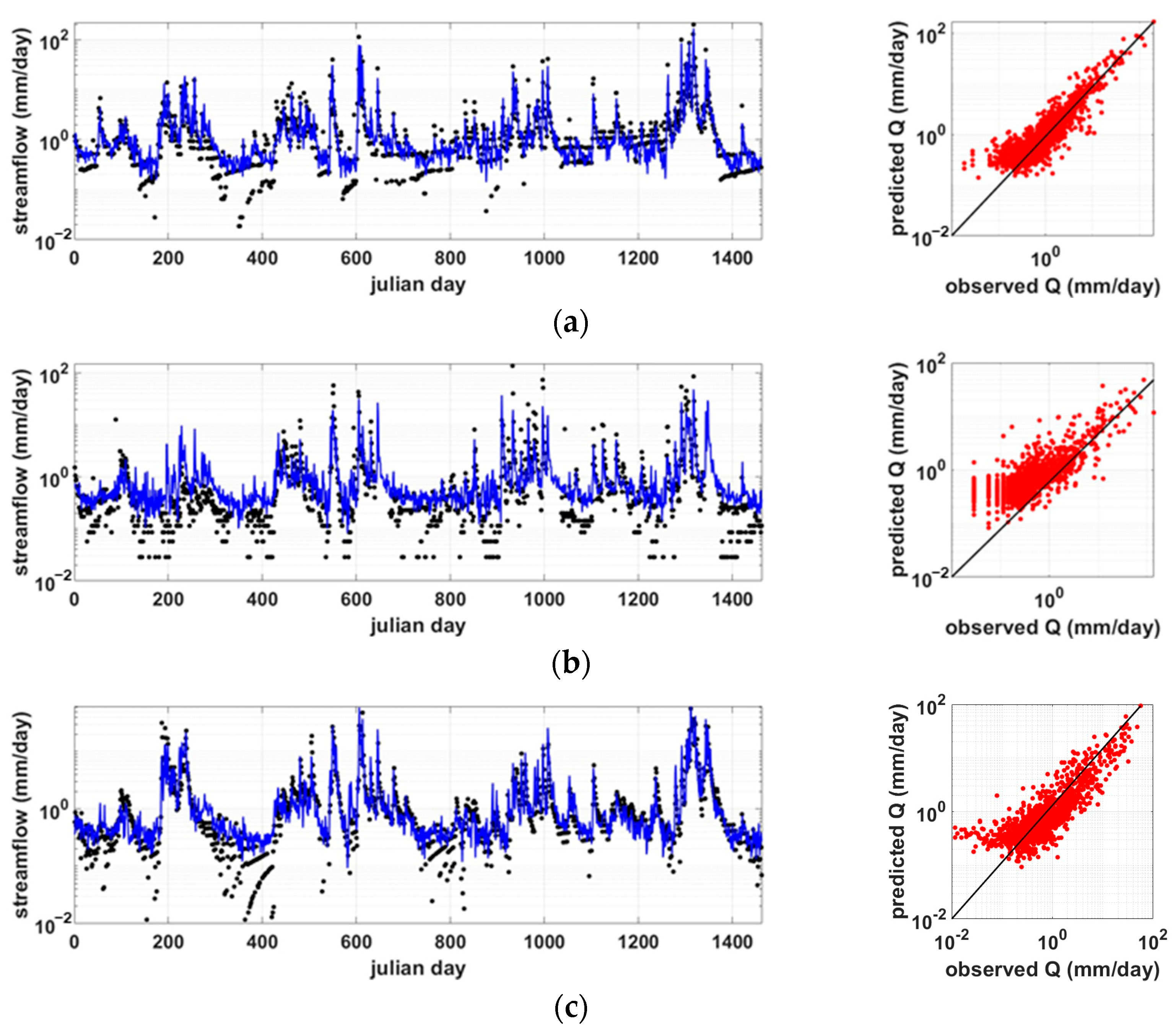
3.1. Predictions in Ungagued Basins Using Meteorological Data and LSTM+RF Combination

Inspired by the regionalization approach, we learned a combined model of RNN and DT-based algorithms by integrating information from multiple gauged basins to predict streamflow in ungauged basins. Figure 3 shows the result of the LSTM+RF combined model trained by the learning strategy of scheme M. Basins 7, 21, and 25 were assumed to be ungauged basins, respectively, and meteorological data and streamflow data from the remaining basins were used as learning data for the model. The left panel of Figure 3 plots observed and simulated streamflow over time, and the red dots in the right panel are Q-Q plots of observed and simulated streamflow. The result of considering Basin 21 as an ungauged basin shows the best performance in the LSTM+RF model of scheme M (R2 = 0.89182, NSE = 0.88258). The result of Basin 7 shows the most inferior performance (R2 = 0.53084, NSE = 0.44618). The result of Basin 25 shows the average performance among the results of applying the LSTM+RF model of scheme M to 25 ungauged basins (R2 = 0.76696, NSE = 0.69141). R2 is the coefficient of determination, and NSE is the Nash-Sutcliffe model efficiency coefficient [36]. The threshold for NSE for good performance is between 0.5 and 0.65 [37,38]. Considering the fact that only preceding meteorological data was used as the input data, the prediction performance of ungauged basins was relatively good, except for the period when the streamflow was very small.

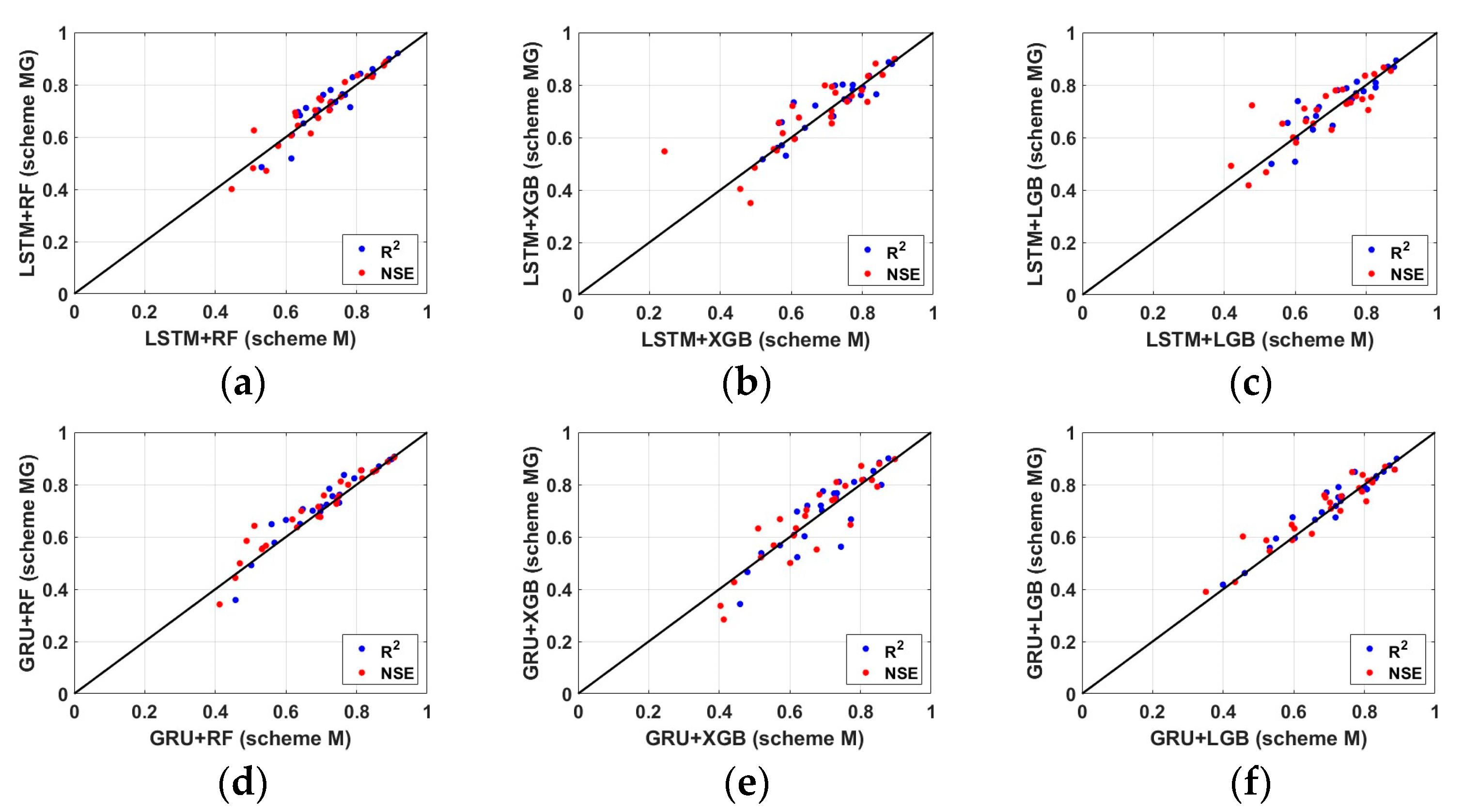
3.2. Comparison of Scheme M and MG

In this section, scheme M and scheme MG are compared. Scheme M is a learning strategy that predicts streamflow in an ungauged basin by inputting only meteorological data, and scheme MG is a learning strategy that predicts an ungauged basin using meteorological data and terrain information. First, the histogram of the annual average meteorological data and terrain data of the 25 basins are shown in Figure 4. The distributions of annual average precipitation, curve number, saturated hydraulic conductivity, and impervious rate are appropriately scattered, but it can be found that the spatial variability of the annual average potential evapotranspiration and basin area is relatively small.

Figure 5 shows the prediction performance of streamflow in 25 ungauged basins derived from each learning strategy and model. One dot in each panel represents the prediction performance of one ungauged basin derived from a particular model. Although there are deviations depending on the watershed, it can be found that the performance of scheme MG is slightly better than that of scheme M in all models. In other words, these results mean that adding topographical information to the prediction model has a slightly positive contribution to improving the prediction performance of ungauged basins rather than using only meteorological data.

In order to further investigate the effect of topographical information on the prediction of ungauged basins, feature importance was extracted from the DT-based algorithm. Feature importance is quantified by measuring how much the performance evaluation index is reduced when predicted with random noise only for the feature (i.e., the input data) of interest. The lower the accuracy, the more important that feature is for prediction, so it is called the mean decrease accuracy (MDA). In this study, MDA was calculated using the permutation importance method in the Scikit-learn package of Python, and the result was normalized and shown in Figure 6.

It can be found that there is almost no deviation by model or by watershed, and this result means that the relative influence of the input data on the prediction of the ungauged basin does not differ greatly depending on the model and watershed. When trying to predict the streamflow of the day, it can be seen that the streamflow first predicted from the preceding meteorological data using RNN has the greatest effect. This indicates that about 70% of streamflow on the day can be explained by preceding meteorological data. In addition, the relative influence of the meteorological data of the day was about 25%, and the relative importance of the topographical information of the watershed was found to be around 5%. The result of this feature’s importance can be analyzed because there is no overall great heterogeneity in meteorological and topographical characteristics between the target watersheds applied in this study. If watersheds with more diverse meteorological or topographical characteristics are included, it is highly probable that features of importance similar to those in Figure 6 will not appear. However, on the flip side, it is difficult to guarantee that the accuracy of the models will be maintained at the same level as in this study if the models are trained by putting watersheds with very heterogeneous meteorological and topographical characteristics into one basket. Therefore, the result of the feature importance shown in Figure 6 could be interpreted as indicating that the level of prediction performance shown in Figure 5 can be expected when applied to an ungauged basin showing the meteorological and topographical characteristics of the range covered in Figure 4. For reference, it can be seen that the relative importance of impervious rate is the highest among topographical characteristics.

In order to examine the predictive performance of scheme M and scheme MG in more detail, we looked at the observed flow duration curve (FDC) and the predicted FDC. FDC, which describes the exceedance probability of streamflow, is one of the most important indicators of hydrologic processes in a watershed [39,40]. To strengthen our analysis, we divided the observed and predicted FDC into three exceedance probability intervals (see

Table 2. Segment classification for each range of flow exceedance probabilities.

Segment	Hydrological Condition Class	Flow Exceedance Probability Range
Segment H	High flow condition	[0, 0.33]
Segment N	Normal flow condition	[0.33, 0.67]
Segment L	Low flow condition	[0.67, 1]

) and compared the prediction performance under the separated hydrological conditions. Among the hydrological conditions of the three sections, the percent bias (pBias) of the streamflow corresponding to the low flow section (segment L in Table 2) was calculated and presented in Figure 7.

Both scheme M and scheme MG reproduce the observed FDC relatively well in the hydrologic conditions corresponding to segment H and segment N but overestimate the streamflow in the section corresponding to segment L (i.e., it can be found that pBias > 100). In segment L, hydrological processes in the watershed are driven by evapotranspiration and percolation rather than rainfall. As shown in Figure 6, since the relative importance of PET and Ks is very small compared to rainfall, it is difficult for the model to adequately express the hydrological cycle process driven by evapotranspiration and percolation. These results indicate that the model constructed in this study has limitations in properly implementing the streamflow in the ungauged basin during the dry period. The reasons for this may be various, but first of all, the limitation of observational data will be one of the most important reasons. As shown in Figure 3, small values among the observed streamflow data are recorded as constant values in steps. This means that the reliability of the streamflow observation data during the dry season is not high. It is reported that it is difficult for RNNs to learn and reproduce the behavior with a constant streamflow value [23]. Nevertheless, the results in Figure 7 indicate that scheme MG shows better performance than scheme M. This suggests that the additional application of terrain information using DT-based algorithms contributes more to predicting streamflow in the dry period than in the wet period or normal period.

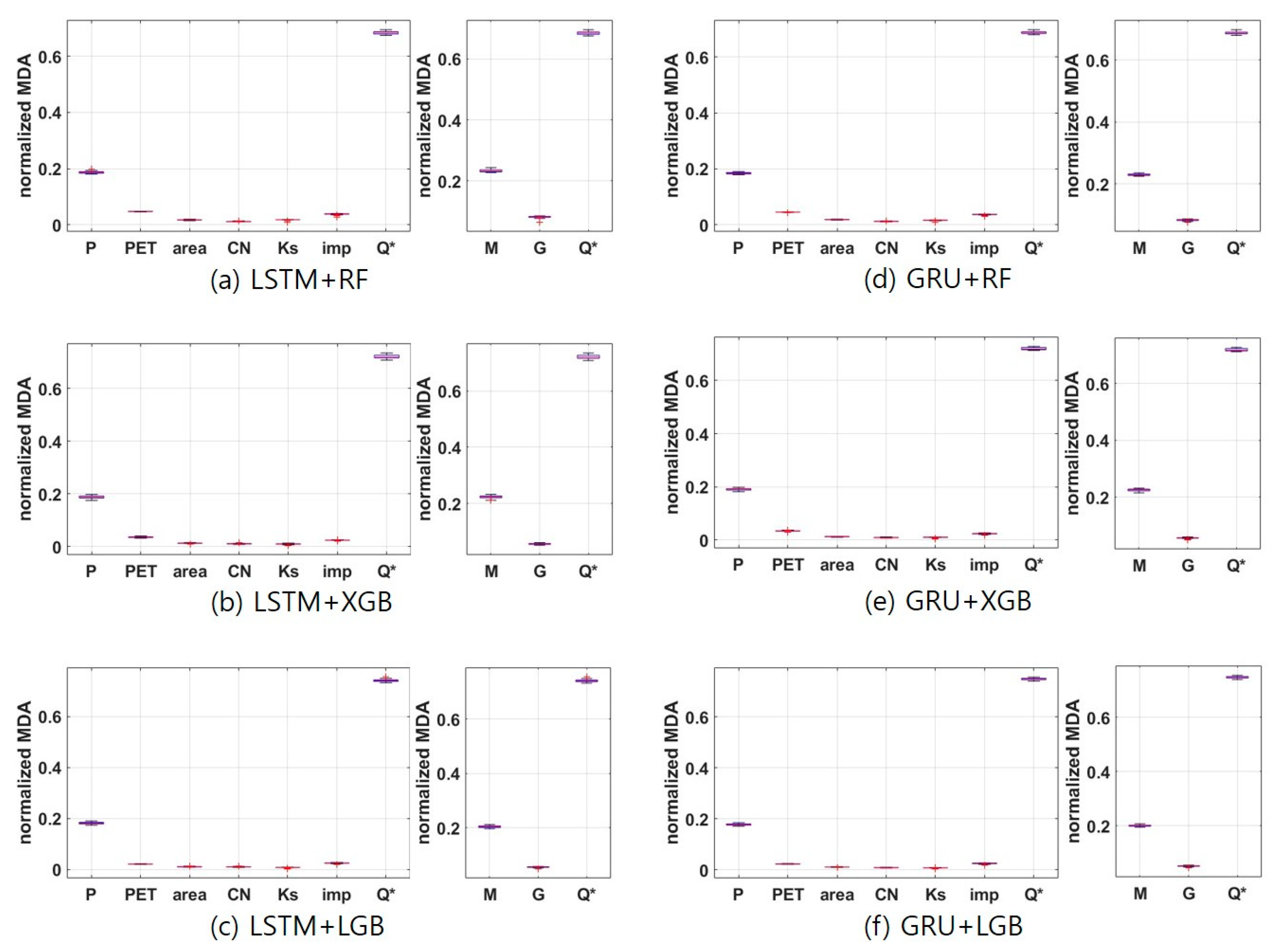
3.3. Comparison between Algorithms of Scheme MG

In this section, we examined the performance of streamflow predicted by the models learned by scheme MG in 25 ungauged basins. From the results of all ungauged basins and models, R2 showed a distribution of 0.3432 (GRU+XGB at Basin 23) to 0.9202 (LSTM+RF at Basin 1), and the average R2 for the 25 ungauged basins was 0.7016 (GRU+XGB) to 0.7338 (LSTM+RF). For NSE, the lowest performance (NSE = 0.2840) was found in Basin 10 with GRU+XGB, and the highest performance (NSE = 0.9035) was recorded in Basin 5 with GRU+RF. The average NSE for the 25 ungauged basins ranged from 0.6672 (GRU+XGB) to 0.7032 (GRU+LGB). Figure 8 shows the NSE performance of the models.

From the results in Figure 8, it can be seen that the model with the best prediction performance is LSTM+LGB. The range of NSE for the 25 ungauged basins ranged from 0.4175 to 0.8666, and the average NSE was 0.6972. Of the 25 ungauged basins, 19 watersheds (76%) had an NSE of 0.65 or higher, and 88% of the 25 watersheds had an NSE of 0.5 or higher, which is the minimum prediction accuracy. The model with the worst prediction performance was GRU+XGB. The NSE ranged from 0.2840 to 0.8972, and the average NSE was 0.6672. An NSE of 0.65 or greater was obtained in 56% of the applied watersheds; the number of watersheds with an NSE of 0.5 or greater was 22. In the case of GRU+XGB, a particularly bad NSE was recorded in Basin 10. In addition to Basin 10, Basin 7, and Basin 23 performed unsatisfactorily in all models. Interestingly, while GRU+XGB was the worst-performing model, NSE in the best-performing watershed was better than LSTM+LGB, which was the best-performing model. This fact underscores the need to test in as many watersheds as possible when determining the superiority of a model’s performance.

4. Discussion

Hybrid models combining machine learning and deep learning techniques have been applied in studies to forecast streamflow in gauged basins [21,22], but most studies that attempt to predict streamflow in ungauged watersheds apply machine learning techniques such as Random Forest or use deep learning techniques such as LSTM [23,24,26,27,28,30]. In this study, deep learning techniques were used to initially predict the behavior of streamflow itself, and then machine learning techniques linked to meteorological data and watershed characteristics were used to finally predict streamflow. The main innovation of this study is that it attempts a framework that sequentially combines both approaches to predict streamflow in ungauged basins.

In this chapter, we further investigated and discussed the relationship between the influence of input data on PUB and the topographical characteristics of the watershed. Figure 9 shows the relationship between the feature importance of each of the six models as determined by the learning strategy of scheme MG and the topographical characteristics of the watershed. The horizontal axis of each panel is the value of the watershed area, curve number, saturated hydraulic conductivity, and impervious rate, respectively. The vertical axis consists of normalized MDAs of annual precipitation, annual potential evapotranspiration, watershed area, curve number, saturated hydraulic conductivity, impervious rate, and the first predicted output by RNN from previous meteorological data. The linear relationship between the topographical characteristics of the watershed and the normalized MDA of the corresponding input features was considered significant only when the p-value was less than 0.05.

Looking at the significant relationship, the importance of Ks in streamflow prediction decreased as the CN increased, and the importance of Ks increased as Ks increased. These results indicate that the importance of soil characteristics represented by the saturated hydraulic conductivity in this study increased as runoff was less likely to occur due to the topographical characteristics of the basin. In addition, as the impervious rate of the watershed increased, its importance decreased, and the importance of the first prediction output by RNN increased. This indicates that the higher the impervious rate, the lower the effect of the impervious rate on the streamflow prediction, but the higher the effect of the preceding meteorological conditions. That is, it can be recognized that as the impervious rate of a watershed increases, the preceding meteorological characteristics play a more important role in predicting streamflow.

Figure 10 is the result of examining the relationship between the PUB performance of the six models by scheme MG and the meteorological and topographical characteristics of the watershed. No significant difference was found in model performance in response to changes in annual precipitation, annual potential evapotranspiration, or dry index. In addition, topographical characteristics such as area, curve number, saturated hydraulic conductivity, and impervious rate did not have a significant effect on the model’s performance. This means that distortion due to meteorological and watershed characteristics did not occur in the performance results of the constructed models.

5. Conclusions

In this study, the applicability of a model combining a recurrent neural network and a decision tree-based algorithm was investigated to predict river flow in an ungauged basin. Using the meteorological and river runoff data of 25 watersheds in Korea, the process of integrating data from 24 gauged basins and predicting river runoff in the remaining one ungauged basin from the learned model was repeated a total of 25 times.

After the river runoff of the day was first predicted by the recurrent neural network from the preceding meteorological data, the river runoff was finally predicted by combining the first predicted river runoff data, the day’s meteorological data, and the terrain features of the basin with a decision tree-based algorithm. In this study, LSTM and GRU were applied to recurrent neural networks, and Random Forest, XGBoost, and LightGBM were applied to decision tree-based algorithms, respectively. From these numerical experiments, how the inclusion of topographical information affects the prediction performance of ungauged basins using data-driven models and the performance differences between commonly applied deep learning and machine learning models were investigated.

The prediction performance of the ungauged basin achieved from the model learned by integrating the information of multiple gauged basins was above the applicable threshold level, regardless of the two learning strategies applied in this study. These results reveal that the river flow in the ungauged basin can be well predicted using the data-driven model. However, these results are based on the premise that data from watersheds with similar climatic and topographical conditions were used during model learning. Therefore it would be desirable to apply them to ungauged basins within the learned range. One clear finding from this study is that the proposed framework has the advantage of explicitly incorporating the topographic information of a watershed by combining a decision tree-based algorithm with a recurrent neural network, which has already been shown to perform well in streamflow prediction in ungauged watersheds, and more clearly quantifying the importance of the incorporated topographic information.

In this study, it was recognized that the additional use of topographical data did not significantly improve the prediction performance of ungauged basins, and the importance of the added topographical data in the model prediction process was not high. However, it was confirmed that it was slightly helpful in improving the river runoff prediction performance in the dry season. However, the combination of recurrent neural networks and decision tree-based algorithms applied in this study still exposed limitations in predicting dry season river runoff in ungauged basins. If we pay attention to the fact that the hydrologic process of the watershed is different in the dry and wet seasons, it is expected that preparing a strategy to learn by distinguishing the dry and wet seasons in future studies can help improve the prediction performance in the ungauged basin. Also, more large sample data sets, including satellite data, are now being provided for training. These opportunities could facilitate the utilization of data-driven models in PUBs and will require more research and some adjustments to current approaches. In addition, research on proper hyperparameter estimation for data-driven models will need to be conducted in the future.

References

1. Schulla, J. LModel Description WaSiM (Water Balance Simulation Model), Completely Revised Version 2012. Last Change: 19 June 2012. 2012. Available online: http://www.wasim.ch/downloads/doku/wasim/wasim_2012_ed2_en.pdf (accessed on 1 March 2022).
2. Hengl, T.; Mendes de Jesus, J.; Heuvelink, G.; Ruiperez Gonzalez, M.; Kilibarda, M.; Blagotic, A.; Shangguan, W.; Wright, M.; Geng, X.; Bauer-Marschallinger, B.; et al. SoilGrids250m: Global gridded soil information based on machine learning. PLoS ONE 2017, 12, e0169748. [Google Scholar] [CrossRef] [PubMed] [Green Version]
3. Wood, E.; Roundy, J.; Troy, T.; van Beek, L.; Bierkens, M.; Blyth, E.; de Roo, A.; Döll, P.; Ek, M.; Famiglietti, J.; et al. Hyper resolution global land surface modeling: Meeting a grand challenge for monitoring Earth’s terrestrial water. Water Resour. Res. 2011, 47, W05301. [Google Scholar] [CrossRef]
4. Worldbank. Assessment of the State of Hydrological Services in Developing Countries. 2018. Available online: https://www.gfdrr.org/sites/default/files/publication/state-of-hydrological-services_web.pdf (accessed on 1 March 2022).
5. USGS. Streamgage History. 2018. Available online: https://water.usgs.gov/nsip/history.html (accessed on 1 March 2022).
6. Fekete, B.; Robarts, R.; Kumagai, M.; Nachtnebel, H.; Odada, E.; Zhulidov, A. Time for in situ renaissance. Science 2015, 349, 685–686. [Google Scholar] [CrossRef] [PubMed]
7. Hrachowitz, M.; Savenije, H.; Blöschl, G.; McDonnell, J.; Sivapalan, M.; Pomeroy, J.; Arheimer, B.; Blume, T.; Clark, M.; Ehret, U. A decade of predictions in ungauged basins (pub)—A review. Hydrol. Sci. J. 2013, 58, 1198–1255. [Google Scholar] [CrossRef]
8. Guo, Y.; Zhang, Y.; Zhang, L.; Wang, Z. Regionalization of hydrological modeling for predicting streamflow in ungauged catchments: A comprehensive review. WIREs Water 2021, 8, e1487. [Google Scholar] [CrossRef]
9. Young, P.; Beven, K. Data-based mechanistic modelling and the rainfall-flow non-linearity. Environmetrics 1994, 5, 335–363. [Google Scholar] [CrossRef]
10. Remesan, R.; Mathew, J. Hydrological Data Driven Modelling: A Case Study Approach; Springer International Publishing: New York, NY, USA, 2014; Volume 1. [Google Scholar]
11. Halff, A.; Halff, H.; Azmoodeh, M. Predicting Runoff from Rainfall Using Neural Networks. In Engineering Hydrology; ASCE: Reston, VA, USA, 1993; pp. 760–765. [Google Scholar]
12. Rumelhart, D.; Hinton, G.; Williams, R. Learning Internal Representations by Error Propagation (No. ICS-8506); California University of San Diego, La Jolla Institute for Cognitive Science: San Diego, CA, USA, 1986. [Google Scholar]
13. Carriere, P.; Mohaghegh, S.; Gaskar, R. Performance of a Virtual Runoff Hydrographic System. Water Resour. Plan. Manag. 1996, 122, 120–125. [Google Scholar]
14. Hochreiter, S.; Schmidhuber, J. Long Short-Term Memory. Neural Comput. 2017, 9, 1735–1780. [Google Scholar] [CrossRef]
15. Cho, K.; van Merrienboer, B.; Bahdanau, D.; Bougares, F.; Schwenk, H.; Bengio, Y. Learning Phrase Representations using RNN Encoder-Decoder for Statistical Machine Translation. arXiv 2014, arXiv:1406.1078. [Google Scholar] [CrossRef]
16. Shi, X.; Chen, Z.; Wang, H.; Yeung, D.; Wong, W.; Woo, W. Convolutional LSTM Network: A Machine Learning Approach for Precipitation Nowcasting. In Advances in Neural Information Processing Systems; MIT Press: Cambridge, MA, USA, 2015; Volume 28, pp. 802–810. [Google Scholar]
17. Tao, Y.; Gao, X.; Hsu, K.; Sorooshian, S.; Ihler, A. A Deep Neural Network Modeling Framework to Reduce Bias in Satellite Precipitation Products. J. Hydrometeoroly 2016, 17, 931–945. [Google Scholar] [CrossRef]
18. Fang, K.; Shen, C.; Kifer, D.; Yang, X. Prolongation of SMAP to Spatiotemporally Seamless Coverage of Continental U.S. Using a Deep Learning Neural Network. Geophys. Res. Lett. 2017, 44, 11030–11039. [Google Scholar] [CrossRef] [Green Version]
19. Assem, H.; Ghariba, S.; Makrai, G.; Johnston, P.; Gill, L.; Pilla, F. Urban Water Flow and Water Level Prediction Based on Deep Learning. In ECML PKDD 2017: Machine Learning and Knowledge Discovery in Databases; Springer: Cham, Switzerland, 2017; pp. 317–329. [Google Scholar]
20. Zhang, J.; Zhu, Y.; Zhang, X.; Ye, M.; Yang, J. Developing a Long Short-Term Memory (LSTM) based model for predicting water table depth in agricultural areas. J. Hydrol. 2018, 561, 918–929. [Google Scholar] [CrossRef]
21. Granata, F.; Di Nunno, F.; de Marinis, G. Stacked machine learning algorithms and bidirectional long short-term memory networks for multi-step ahead streamfow forecasting: A comparative study. J. Hydrol. 2022, 613, 128431. [Google Scholar] [CrossRef]
22. Di Nunno, F.; de Marinis, G.; Granata, F. Short-term forecasts of streamflow in the UK based on a novel hybrid artificial intelligence algorithm. Sci. Rep. 2023, 13, 7036. [Google Scholar] [CrossRef]
23. Kratzert, F.; Klotz, D.; Brenner, C.; Schulz, K.; Herrnegger, M. Rainfall–runoff modelling using Long Short-Term Memory (LSTM) networks. Hydrol. Earth Syst. Sci. 2018, 22, 6005–6022. [Google Scholar] [CrossRef] [Green Version]
24. Arsenault, R.; Martel, J.; Brunet, F.; Brissette, F.; Mai, J. Continuous streamflow prediction in ungauged basins: Long short-term memory neural networks clearly outperform traditional hydrological models. Hydrol. Earth Syst. Sci. 2023, 27, 139–157. [Google Scholar] [CrossRef]
25. Choi, J.; Won, J.; Jang, S.; Kim, S. Learning enhancement method of Long short-term memory network and its applicability in hydrological time series prediction. Water 2022, 14, 2910. [Google Scholar] [CrossRef]
26. Ayzel, G.; Kurochkina, L.; Abramov, D.; Zhuravlev, S. Development of a Regional Gridded Runoff Dataset Using Long Short-Term Memory (LSTM) Networks. Hydrology 2021, 8, 6. [Google Scholar] [CrossRef]
27. Kratzert, F.; Gauch, M.; Nearing, G.; Klotz, D. Neural Hydrology–A Python library for Deep Learning. J. Open Source Softw. 2022, 7, 4050. [Google Scholar] [CrossRef]
28. Kratzert, F.; Klotz, D.; Herrnegger, M.; Sampson, A.; Hochreiter, S.; Nearing, G. Toward improved predictions in ungauged basins: Exploiting the power of machine learning. Water Resour. Res. 2019, 55, 11344–11354. [Google Scholar] [CrossRef] [Green Version]
29. Li, X.; Khandelwal, A.; Jia, X.; Cutler, K.; Ghosh, R.; Renganathan, A.; Xu, S.; Tayal, K.; Nieber, J.; Duffy, C.; et al. Regionalization in a global hydrologic deep learning model: From physical descriptors to random vectors. Water Resour. Res. 2022, 58, e2021WR031794. [Google Scholar] [CrossRef]
30. Choi, J.; Lee, J.; Kim, S. Utilization of the Long Short-Term Memory network for predicting streamflow in ungauged basins in Korea. Ecol. Eng. 2022, 182, 106699. [Google Scholar] [CrossRef]
31. Allen, R.; Pereira, L.; Raes, D.; Smith, M. Crop Evapotranspiration-Guidelines for Computing Crop Water Requirements-FAO Irrigation and Drainage Paper 56; FAO: Rome, Italy, 1998; Volume 300, p. D05109. [Google Scholar]
32. Won, J.; Kim, S. Future drought analysis using SPI and EDDI to consider climate change in South Korea. Water Supply 2020, 20, 3266–3280. [Google Scholar] [CrossRef]
33. Schmidhuber, J. Deep learning in neural networks: An overview. Neural Netw. 2015, 61, 85–117. [Google Scholar] [CrossRef] [Green Version]
34. Srivastave, N.; Hinton, G.; Krizhevsky, A.; Sutskever, I.; Salakhutdinov, R. Dropout: A simple way to prevent neural networks from overfitting. J. Mach. Learn. Res. 2014, 15, 1929–1958. [Google Scholar]
35. Turkyilmazoglu, M. Accelerating the convergence of Adomian decomposition method (ADM). J. Comput. Sci. 2019, 31, 54–59. [Google Scholar] [CrossRef]
36. Nash, J.; Sutcliffe, J. River flow forecasting through conceptual models. part I—A discussion of principles. J. Hydrol. 1970, 10, 282–290. [Google Scholar] [CrossRef]
37. Ritter, A.; Munoz-Carpena, R. Performance evaluation of hydrological models: Statistical significance for reducing subjectivity in goodness-of-fit assessments. J. Hydrol. 2013, 480, 33–45. [Google Scholar] [CrossRef]
38. Kim, R.; Won, J.; Choi, J.; Lee, O.; Kim, S. Application of Bayesian approach to parameter estimation of TANK model: Comparison of MCMC and GLUE methods. J. Korean Soc. Water Environ. 2020, 36, 300–313. [Google Scholar]
39. Ruiz-Perez, G.; Gonzalez-Sanchis, M.; Del Campo, A.; Frances, F. Can a parsimonious model implemented with satellite data be used for modelling the vegetation dynamics and water cycle in water-controlled environments? Ecol. Model. 2016, 324, 45–53. [Google Scholar] [CrossRef] [Green Version]
40. Choi, J.; Won, J.; Lee, O.; Kim, S. Usefulness of global root zone soil moisture product for streamflow prediction of ungauged basins. Remote Sens. 2021, 13, 756. [Google Scholar] [CrossRef]
Figure 1. Location of study watersheds. Red ▲ means the location of weather observation sites.
Water 15 02485 g001
Figure 2. The process flow diagram for this study.
Water 15 02485 g002
Figure 3. Test results from LSTM-RF with scheme M. In the left panel, the black point is the observed river runoff, and the blue solid line is the river runoff predicted by the model. (a) Basin 21, (b) Basin 7, and (c) Basin 25.
Water 15 02485 g003
Figure 4. Histogram for meteorological and geographic data in 25 watersheds.
Water 15 02485 g004
Figure 5. Performance metrics of scheme M and MG. (a) LSTM+RF; (b) LSTM+XGB; (c) LSTM+LGB; (d) GRU+RF; (e) GRU+XGU; (f) GRU+LGB.
Water 15 02485 g005
Figure 6. Feature importance. In the left panel of the figure, P is the daily precipitation, PET is the daily potential evapotranspiration, area is the watershed area, CN is the curve number, Ks is the saturated hydraulic conductivity, imp is the impervious rate, and Q* is the streamflow first predicted by RNN. In the right panel of the figure, M is the sum of the normalized MDAs of P and PET, which means the importance of meteorological features, and G is the sum of the normalized MDA values for the terrain features (i.e., area, CN, Ks, and imp).
Water 15 02485 g006
Figure 7. Flow duration curve and pBias in the low streamflow range. (a) Flow duration curves at Basin 17; (b) pBias in the low streamflow range.
Water 15 02485 g007
Figure 8. Performance of scheme MG.
Water 15 02485 g008
Figure 9. Effect of watershed topographical characteristics on model feature importance.
Water 15 02485 g009
Figure 10. Effect of watershed climate and geographic characteristics on model performance.
Water 15 02485 g010aWater 15 02485 g010b