
Abstract
To counter response distortions associated with the use of rating scales (a.k.a. Likert scales), items can be presented in a comparative fashion, so that respondents are asked to rank the items within blocks (forced-choice format). However, classical scoring procedures for these forced-choice designs lead to ipsative data, which presents psychometric challenges that are well described in the literature. Recently, Brown and Maydeu-Olivares (Educational and Psychological Measurement 71: 460–502, 2011a) introduced a model based on Thurstone’s law of comparative judgment, which overcomes the problems of ipsative data. Here, we provide a step-by-step tutorial for coding forced-choice responses, specifying a Thurstonian item response theory model that is appropriate for the design used, assessing the model’s fit, and scoring individuals on psychological attributes. Estimation and scoring is performed using Mplus, and a very straightforward Excel macro is provided that writes full Mplus input files for any forced-choice design. Armed with these tools, using a forced-choice design is now as easy as using ratings.
Typical questionnaire and survey items are presented to respondents one at a time (single-stimulus items), which often leads to indiscriminate endorsement of all desirable items by respondents, resulting in systematic score inflation. Forced-choice response formats were designed to reduce such biases by forcing people to choose between similarly attractive options. In forced-choice questionnaires, items are presented in blocks of two, three, four, or more items at a time, and respondents are asked to rank the items within each block according to some instruction (e.g., in terms of how well the items describe their behavior or attitudes). Sometimes, the respondents are asked to indicate only the top and the bottom ranks (e.g., to select one item that best describes them and one that least describes them).
One special case of forced-choice is the so-called multidimensional forced-choice (MFC), in which each item is assumed to measure only one psychological attribute, and all items within a block measure different attributes. MFC questionnaires are popular in the psychological assessment industry because it is believed that this format is more robust against response sets, halo effects, and impression management, and experimental evidence supports these ideas (e.g., Bartram, 2007; Cheung & Chan, 2002; Christiansen, Burns, & Montgomery, 2005; Jackson, Wroblewski, & Ashton, 2000).
The standard scoring used with forced-choice questionnaires involves adding the inverted rank orders of items within blocks to their respective scales. As a fixed number of points are allocated in every block, the total number of points on the test is the same for every individual (ipsative data). In other words, one scale score can be determined from the remaining scales. Ipsativity leads to some highly undesirable consequences, namely:
-
1.
Scores are relative rather than absolute; therefore, while meaningful intraindividual interpretations can be made, comparisons between individuals are problematic.
-
2.
Construct validity is distorted. Because one scale can be determined from the remaining scales, the scales’ correlation matrix has one zero-eigenvalue that prevents the use of factor analysis. More importantly, the average scale intercorrelation can be derived exactly from the number of scales, and it must be negative, regardless of the true relationships between the measured attributes (see, e.g., Clemans, 1966).
-
3.
Criterion-related validity is distorted. Due to zero variance of the total score, the correlations between a questionnaire’s scales and any external criterion must sum to zero (e.g., Clemans, 1966). Consequently, any positive correlations with the criterion must be compensated by spurious negative correlations, and vice versa.
-
4.
Reliability estimates are distorted. Classical reliability coefficients are not appropriate for forced-choice questionnaires, because ipsative data violates the assumptions underlying them, such as the independence of measurement errors (e.g., Meade, 2004).
Much has been written about the problems of ipsative data (for an overview, see Brown, 2010; see also Baron, 1996), and as a result, forced-choice tests have been controversial. These psychometric problems, however, are due to the inappropriateness of classical procedures for scoring MFC items, not to the forced-choice format per se (Brown & Maydeu-Olivares, 2011a). The problem with classical scoring is that it completely disregards the response process that individuals engage in when making forced choices. However, because forced-choice blocks are simply sets of rankings (or partial rankings), existing response models for ranking data can be adapted for modeling and scoring forced-choice questionnaire data.
Drawing on Thurstone’s law of comparative judgment (Thurstone, 1927, 1931), Brown and Maydeu-Olivares (2011a) recently introduced an item response theory (IRT) model capable of modeling responses to any MFC questionnaire (Thurstonian IRT model). Brown (2010) showed that modeling preference decisions in forced-choice questionnaires using this model yields scores on measured attributes that are free from the problems of ipsative data. The Thurstonian IRT model is a multidimensional item response model with some special features that can be straightforwardly estimated using the general modeling software Mplus (L. K. Muthén & Muthén 1998–2010), which also conveniently estimates trait scores for individuals. The estimation is fast; however, programming these models in Mplus is tedious and error-prone, except for very small models, as one needs to impose parameter constraints that reflect the within-block patterned relationships among items. However, the model is conceptually so simple that the Mplus programming can be easily automated. With this article, we provide a very simple Excel macro that writes the Mplus syntax necessary to fit the IRT model to any MFC questionnaire. Furthermore, we provide a detailed tutorial on how to model different types of MFC questionnaires and how to score respondents on the measured attributes.
The article is organized as follows. We begin by providing general theory for the Thurstonian IRT model. Thus, we describe how to code responses to forced-choice questionnaires and how to link these responses to the attributes that the questionnaire is intended to measure, building a factor-analytic model with binary variables (an IRT model). We describe some special features of these models, as well as the identification constraints necessary to estimate them. We also show how general multidimensional IRT theory can be applied to score individuals. Next, we provide an extended tutorial for modeling specific forced-choice designs using simple numerical examples with simulated data. All of the data sets and Mplus input files are available for download. In this tutorial, we cover different block sizes (items presented in pairs, triplets, or quads) and their common and specific features. We cover both full-ranking and partial-ranking designs. Partial rankings arise when only the top and bottom ranking choices (i.e., “most” and “least” choices) are requested, in order to simplify the task of responding to blocks of four or more items. In this case, missing data arise, and we provide an example of how to deal with this using multiple imputation in Mplus.
Thurstonian IRT model
Coding forced-choice responses
Consider a questionnaire consisting of items presented in blocks of n items each. Respondents are asked to rank the items within each block. To code their responses, ñ = n(n – 1)/2 binary outcome (dummy) variables per block are used, one for every pairwise combination of items (Maydeu-Olivares & Böckenholt, 2005). For instance, to code a rank ordering of n = 4 items A, B, C, and D, one needs to consider the outcomes of ñ = 6 pairwise comparisons: whether A was preferred to B, to C, and to D; whether B was preferred to C and to D, and whether C was preferred to D. To reach the ordering {B, A, D, C}, B must be preferred in all pairwise comparisons involving it, and C must not be preferred in any. For each pairwise combination l = {i, k}, a binary variable y l is used to indicate the outcome of the comparison:
The ordering {B, A, D, C} can then be coded using binary outcome variables, as follows in Table 1. Sometimes respondents are only asked to report one item that best describes them and one that least describes them. The partial ranking corresponding to our example above would yield one missing outcome—the ordering of items A and D is not known, as we see in Table 2.
Partial-ranking format results in missing binary outcome variables whenever the block size is four items or more. These outcomes are missing at random (MAR) because the patterns of missing responses do not depend on the missing outcomes; that is, the outcome of the comparison between items that have not been selected as “most” or “least” is missing not because any particular preference would be more or less likely, but because no preference was recorded. However, the outcome is not missing completely at random (MCAR), because the patterns of missing responses can be deduced from the observed choices made in the block. For instance, in the example above, it is known from the observed responses (item B selected as “most” and item C as “least”) that the comparison between the two remaining items, A and D, will not be recorded, so that the binary outcome {A, D} will be missing. Thus, given the observed most–least choices, the pattern of missing outcomes is known for each individual.
Modeling preference responses in relation to latent traits
To relate the observed binary outcomes to psychological attributes measured by the questionnaire, we use the notion of item utility—an unobserved psychological value placed on the item by a respondent. The utility of item i is denoted t i . According to Thurstone’s (1927) law of comparative judgment, items’ utilities are assumed to be normally distributed across respondents and to determine preferential choices. That is, given any two items, the respondent deterministically chooses the item with the highest utility. For computational reasons, it is convenient to express Thurstone’s model using differences of utilities. Let y l * denote the (unobserved) difference of utilities for the pair of items l = {i, k}:
Then, Thurstone’s law can be written by relating the observed binary outcome to the unobserved difference of two utilities (we can think of it as a response tendency),
In multitrait questionnaires, utilities of items are assumed to be governed by a set of d psychological attributes (common factors, or latent traits) according to a linear factor analysis model
or, in matrix form,
where η = (η 1, η 2, . . . η d ) is a vector of common attributes, Λ is a matrix of factor loadings, μ is a vector of item intercepts, and ε is a vector of unique factors (specification and measurement errors)—assumed to be mutually uncorrelated. We let Φ = var(η) be the factors’ covariance matrix (for identification, we set all variances equal to 1 so that it is a correlation matrix), and Ψ 2 = var(ε) be the diagonal matrix of the errors’ variances.
Combining Eqs. 2 and 4, we obtain a factor model that links the preference response tendency to the hypothesized common attributes,
where the threshold γ l replaces the difference of the item intercepts: γ l = –(μ i – μ k ). When items are presented in p blocks of size n, there are ñ = n(n – 1)/2 binary outcomes per block, and the total number of binary outcomes in the questionnaire is p × ñ. In matrix form, the (p × ñ) vector of response tendencies y * of the binary outcomes y is written as

Here, γ is a (p × ñ) vector of thresholds;  is a (p × ñ) × d matrix of factor loadings; and
  is a (p × ñ) vector of errors with covariance matrix var
  . The relationships between the matrices
  and
and  of the Thurstonian IRT model and the matrices Λ and Ψ
2 of the factor-analysis model (Eq. 5) describing the relationship between the items and the common attributes they measure are given by
of the Thurstonian IRT model and the matrices Λ and Ψ
2 of the factor-analysis model (Eq. 5) describing the relationship between the items and the common attributes they measure are given by

where A is a block diagonal matrix. When n = 2, each block in A is (1 – 1), whereas when n = 3 and n = 4, they are, respectively
Parameters of the independent-clusters Thurstonian IRT model
Most confirmatory applications assume that each item measures only one trait and that the factor model underlying the item utilities possesses an independent-clusters basis (McDonald, 1999). This factorial simplicity is certainly the aim in typical forced-choice questionnaires, and in what follows, we concentrate on independent-clusters factorial structures. When questionnaire items measure two or more attributes, the general theory in Eq. 6 applies. In this case, the IRT model can be estimated in the same fashion as the independent clusters; however, additional identification constraints are needed (see the Model Identification section). When items i and k measure different attributes, η a and η b (i.e., a multidimensional comparison), Eq. 6 simplifies to
If, instead, i and k measure the same attribute η a (i.e., a one-dimensional comparison), Eq. 6 becomes
Thus, the Thurstonian IRT model with p × ñ binary outcomes contains:
-
1.
p × ñ threshold parameters γ l . One threshold γ l = – (μ i – μ k ) is estimated for each binary outcome (i.e., we do not estimate the original intercepts of utilities).
-
2.
p × n factor loading parameters These are the factor loadings of utilities. Two factor loadings are estimated for each binary outcome—these relate the response tendency to the two attributes measured by the items making up the pairwise comparison. When the block size is n = 2 (i.e., items are presented in pairs), each item is involved in one pairwise comparison only, and therefore each utility’s factor loading appears only once in matrix
 (for an example, see matrix
  in Eq. 21). When the block size is n > 2, each item is involved in n − 1 pairwise comparisons, and therefore each utility’s factor loading occurs more than once (n − 1 times) in matrix
  , forming patterns (for example, see matrices
  for a triplet design in Eq. 19, and for a quad design in Eq. 20).
 -
3.
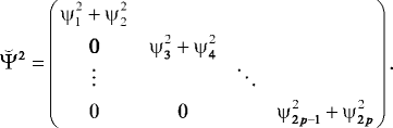
p × n uniqueness parameters ψ i 2 These are the uniquenesses of utilities, and when the block size is n = 2 (i.e., items are presented in pairs), the residual variance matrix var
 is a p × p diagonal matrix:
 (12)
(12)
 (for an example, see matrix
  in Eq.
  , forming patterns (for example, see matrices
  for a triplet design in Eq.
  is a p × p diagonal matrix:

When the block size is n > 2, there is shared variance between binary outcomes involving the same item, and  is a (p × ñ) × (p × ñ) block-diagonal matrix, with the following blocks for n = 3 and n = 4, respectively:


The above special features of matrices  and
and  complete the definition of the Thurstonian IRT model.
Model identification
To identify a Thurstonian IRT model (Eq. 10) built for MFC items that are designed to measure one trait only (also referred to as multi-unidimensional structure in the IRT literature), one needs to set a metric for the latent traits and item errors. The latent traits’ variances are set to 1. To set a metric for item errors, for blocks of size n > 2 (items are presented in triplets, quads, etc.), it suffices to fix the uniqueness of one item per block. Throughout this report, we use the convention of (arbitrarily) fixing the uniqueness of the first item in each block to 1. When the block size is n = 2 (i.e., items are presented in pairs), no item uniqueness can be identified. In this case, it is convenient to fix the uniqueness of each binary outcome (which is the sum of two item uniquenesses, as can be seen from Eq. 12) to 1.
The above constraints are generally sufficient to identify most forced-choice designs. A special case arises when multidimensional pairs (n = 2) are used to assess exactly two attributes (d = 2). Because this model is essentially an exploratory factor model, additional identification constraints need to be imposed on some factor loadings. This case is discussed in Example 4.
When questionnaire items measure two or more attributes, such as in the general case described by Eq. 6, additional constraints may be needed to identify factor loadings, because only their differences can be estimated without constraints. This is similar to the unidimensional model described in Eq. 11, where setting one factor loading is necessary to identify the model (Maydeu-Olivares & Brown, 2010).
Nonidentified models may occasionally arise when item factor loadings within the same block are equal or indistinguishable from the empirical data. This might happen in designs in which positively keyed items measure a small number of attributes, or the attributes are positively correlated, so that the item parameters are more difficult to estimate accurately (Brown & Maydeu-Olivares, 2011a). When the factor loadings λ i and λ k are equal (say, they equal λ), the difference of utilities in Eq. 10 is described by
In this case, the data are sufficiently described by d − 1 differences between each attribute and, say, the last attribute η d . Indeed, for any pair of attributes η a and η b , their difference η a – η b can be written as (η a – η d ) – (η b – η d ). The factor space is therefore reduced, and additional constraints are needed to identify the model. In practice, it may not be easy to spot such empirical underidentification, because no warning of a nonidentified model may be given by Mplus. The researcher needs to examine the program output very carefully to ensure that everything is as expected. Typical signs of the described special case are that estimated factor loadings for one of the factors are close to zero, standard errors of the correlation estimates between that factor and other factors are large, and factor correlations are not as expected (usually too high). In some cases, Mplus might give a warning in the output that “the latent variable covariance matrix (Psi) is not positive definite,” and indicate which factor presents a problem. To remedy this situation, it usually suffices to constrain the factor loadings within each block to be equal (without setting their values), and setting just one correlation between the latent traits to its expected value (e.g., to a value predicted by substantive psychological theory).
Parameter estimation and goodness-of-fit testing using Mplus
After the choices are coded as described above, a multi-unidimensonal model (Eq. 10) or the unidimensional model (Eq. 11) is fitted to the differences of utilities y l *. However, the difference variables y l * are not observed, only their dichotomizations y l using the threshold process in Eq. 3 are observed. Hence, a factor model for binary data (the IRT model) is fitted to the binary outcome variables. All that is needed is a program capable of estimating such a model. The program Mplus (L. K. Muthén & Muthén, 1998–2010) conveniently implements all of the necessary features.
The presence of correlated errors, along with the large number of latent traits typically measured by forced-choice questionnaires, precludes the estimation of the model by full-information maximum likelihood (Bock & Aitkin, 1981). However, the model can be straightforwardly estimated using limited-information methods. Unweighted least squares (ULS) or diagonally weighted least squares (DWLS) can be used to this end, and the difference between the two is negligible (Forero, Maydeu-Olivares, & Gallardo-Pujol, 2009). When estimating models with discrete dependent variables, Mplus offers two choices of parameterization, unstandardized and standardized parameters, referred to as “theta” and “delta,” respectively. The Thurstonian IRT model is estimated as a factor analysis for binary data using the “theta” parameterization with the additional constraints on  and
and  described above. Because contrast matrices A are not of full rank (Maydeu-Olivares & Böckenholt, 2005), the matrix of residual variances and covariances
  is also not of full rank. This is by design, and therefore for all forced-choice models Mplus will give a warning that “the residual covariance matrix (theta) is not positive definite.”
The goodness of fit of the model to the tetrachoric correlations is tested by Mplus. The program provides mean or mean and variance Satorra–Bentler (1994) adjustments to the ULS/DWLS fit functions. Mean and variance adjustments provide more accurate p values at the expense of more computations. The mean and variance adjustment for the ULS estimation is denoted as “estimator” ULSMV in Mplus, and it is denoted WLSMV for the DWLS estimation. All models presented in this article are estimated with Mplus using ULS with mean- and variance-corrected Satorra–Bentler goodness-of-fit tests (ULSMV).
With this article, we supply an Excel macro that automates writing the full code, so that all of the necessary parameter constraints are specified. Moreover, the Excel macro takes care of specifying the estimator and parameterization.
When the number of items per block is n > 2, a correction to the degrees of freedom is needed when testing model fit. This is because for each block there are r = n(n – 1)(n – 2)/6 redundancies among the thresholds and tetrachoric correlations estimated from the binary outcome variables (Maydeu-Olivares, 1999). With p ranking blocks in the questionnaire, the number of redundancies is p × r. Thus, when n > 2, one needs to subtract p × r from the degrees of freedom given by Mplus to obtain the correct p value for the test of exact fit. Goodness-of-fit indices involving degrees of freedom in their formula, such as the root mean square error of approximation (RMSEA)
also need to be recomputed using the correct number of degrees of freedom. When n = 2, no degrees-of-freedom adjustment is needed; the p value and RMSEA printed by the program are correct.
Estimation of individuals’ scores
The item characteristic function (ICF) of the binary outcome variable y l described, which is the result of comparing item i measuring trait η a and item k measuring trait η b , is given by
In this function, γ l is the threshold for binary outcome, λ i and λ k are the items’ factor loadings, and ψ i 2 and ψ k 2 are the items’ uniquenesses. Therefore, the Thurstonian IRT model can be seen as an extension of the normal ogive IRT model (Lord, 1952) to situations in which items are presented in blocks and the underlying structure is multidimensional. A special feature of this model is that, when block size is n > 2, the item characteristic functions are not independent (local independence conditional on the latent traits does not hold). Rather, there are patterned covariances among the binary outcomes’ residuals, as shown in Eqs. 13 and 14.
After the model parameters have been estimated, respondents’ attributes can be estimated using a Bayes modal procedure (maximum a posteriori, or MAP estimator)
and this is conveniently implemented in Mplus as an option within the estimation process (B. O. Muthén, 1998–2004). When using Eq. 18, Mplus makes the simplifying assumption that local independence holds. The use of this simplification for scoring individuals has little impact on the accuracy of the estimates (Maydeu-Olivares & Brown, 2010).
Tutorial on writing Mplus code with the excel macro
Despite the fact that the factorial models (Eqs. 10 and 11) underlying forced-choice comparisons are simple, the programming is complicated by the fact that the factor loadings and uniquenesses for the differences y
* must be expressed as linear functions of the factor loadings and uniquenesses of the items. There are also constraints on the parameter matrices  and
and  , which depend on block size, and writing them out is tedious and error prone. In subsequent sections, we will provide details on how to estimate the model for a set of examples (using blocks of different sizes, different numbers of common attributes, etc.) using the supplied Excel macro that writes the full Mplus syntax.
Coding the data
Mplus expects the forced-choice responses to be coded using binary outcomes (dummy variables), as described in this article: one line per individual. If, however, the forced-choice data have been recorded using rank orders of items within each block, or reversed rank orders, as is often the case with already “ipsative scored” items, the responses should be recoded as binary outcomes of pairwise comparisons. Recall that this coding requires each ranking block of size n to be presented as ñ = n(n – 1) / 2 pairwise comparisons {i, k}, each of which takes value 1 if i was preferred to k, and 0 otherwise. This recoding can be easily performed using standard statistical software prior to modeling with Mplus. Alternatively, DEFINE commands can be used to recode the data within Mplus. For rank-orderings, binary outcomes of all pairwise combinations of n items are computed as “i1i2 = i2-i1;” (for ipsative item scores, we use “i1i2 = i1-i2;”), and then all outcomes are cut as binary variables using “CUT i1i2 i1i3 . . . (0);”.
For incomplete rankings, preferences between all items not selected as “most” or “least” in blocks of size n ≥ 4 should be coded as missing data, using conditional statements: for example, “IF (i2 GT i1) THEN i1i2 = 1; IF (i2 LT i1) THEN i1i2 = 0; IF (i2 EQ i1) THEN i1i2 = _MISSING;”. In addition, when missing data are present, the missing responses have to be imputed prior to model estimation. This is described in Example 2.
Writing model syntax
To aid programming of Thurstonian IRT models, we created an Excel macro that can be downloaded from http://annabrown.name/software. Excel was chosen because it is widely available, and because it enables simple “copying and pasting” of questionnaire keys, correlation matrices, and so forth, straight into the provided cells. At Step 1, the macro just requires as input the name of the data file containing the binary outcomes (the data file may contain additional variables), the name of a file in which to save the respondents’ scores (this is optional), the number of forced-choice blocks in the questionnaire, and the block size. At Step 2, the user is required to enter the number of attributes measured by the questionnaire, and a table is also provided for inserting the questionnaire “key.” The “key” is simply a numbered list of all questionnaire items, and the user has to indicate which attribute (referred to by its number) each item measures. The macro also has an option to indicate any negatively keyed items. These are items designed to represent low attribute scores, such as “I keep in the background” to indicate extraversion. This information is optional and is only used for assigning better (negative) starting values for factor loading parameters. Finally, Step 3 (also optional) enables the user to provide starting values for the attribute correlation matrix. With this information, the Excel macro creates the full Mplus syntax, which can be viewed immediately in Excel, and also copied to a ready-to-execute Mplus input.
Numerical examples
Below we present some numerical examples using simulated data. The examples have been designed for illustration only and are necessarily very short. Synthetic data, available for download together with Mplus input files, were used to better illustrate the behavior of the model. As a general foreword for the following examples, we remind the reader that designing forced-choice measures with a given block size requires careful consideration of several factors—such as the keyed direction of items, the number of measured attributes, and correlations between the attributes (Brown & Maydeu-Olivares, 2011a). In the examples below, all of these factors have been balanced to create very short but fully working “fragments” of forced-choice tests. Such short questionnaires in practice would necessarily yield latent trait estimates with high measurement error. Therefore, these examples should only be used as a guide for modeling longer questionnaires. Examples of applications with real questionnaire data are given in the Concluding Remarks section.
Example 1: block size n = 3, full-ranking response format
Consider a very simple multidimensional forced-choice design using p = 4 blocks of n = 3 items (triplets), measuring d = 3 common attributes. For simplicity, let the first item in each block measure the first common attribute, the second item measure the second attribute, and the third item measure the third attribute, therefore each attribute is measured by four items. We assume that each item measures a single trait and that the traits are possibly correlated (their correlation matrix is Φ ). The data are coded using p × ñ = 4 × 3 = 12 binary outcomes in total.
According to this forced-choice design, the item utilities’ loading matrix Λ in Eq. 4 and the pairwise outcomes’ loading matrix  in Eq. 7 are:

As can be seen, the loading matrix  is patterned, with each utility loading appearing exactly twice. The fact that loadings related to comparisons involving the same items are the same (may differ in sign) need to be written out in Mplus using the MODEL CONSTRAINT command (automatically written by the Excel macro).
The item residual matrix is Ψ2 = diag(ψ
21
, . . . , ψ
212
), and the pairwise outcomes’ residual matrix  is block-diagonal with elements
  , as described in Eq. 13. The other model parameters of the Thurstonian IRT model are the factor correlation matrix Φ and a set of p × ñ thresholds γ. To identify the model, we just need to set trait variances to 1 and set the first uniqueness within each block to 1.
To illustrate the discussion, we generated responses from N = 2,000 individuals using the parameter values shown in Table 3. Some factor loadings shown in that table are larger than unity. This is because these are unstandardized factor loadings. The data were simulated by generating latent traits η with mean zero and correlation matrix Φ, as well as errors  with mean zero and covariance matrix
  , and then computing
  . These difference values were then dichotomized at zero as per Eq. 3. The resulting responses are provided in the file triplets.dat, which consists of 2,000 rows and 12 columns, one for each binary outcome variable.
To create Mplus syntax to test this simple model with the supplied data, one can use the Excel macro. One would need to specify the data file (triplets.dat), the block size (3), the number of blocks (4), and the number of attributes measured (3), and to supply the questionnaire key, which in this example will look as follows: (1, 2, 3, 1x, 2, 3, 1, 2, 3x, 1, 2x, 3). The numbers indicate which trait is measured by each item, and “x” indicates that the item is negatively keyed. The latter type of input is optional, as it is only used to supply better (negative) starting values for factor loading parameters. Also, starting values for correlations between the attributes can optionally be given. Once input is complete, the syntax written by the Excel macro can be saved as an Mplus input file and executed, making sure that the file containing the data is located in the same directory as the Mplus input file. Our syntax file triplets.inp can be found in the supplementary materials; it is also given in Appendix A.
After completing the estimation of the supplied data set, Mplus yields a chi-square test of χ 2 = 30.21 on 43 degrees of freedom. However, each triplet has r = n(n – 1)(n – 2) / 6 = 1 redundancy, and there are four redundancies in total, so that the correct number of degrees of freedom is df = 39, leading to a p value of .84. The RMSEA computed using the formula in Eq. 16 with the correct number of degrees of freedom corresponds, in this case, to the value reported by the program (zero) because the chi-square value is smaller than the df value. The estimated item parameters are reported in Table 3, along with their standard errors. We can see in this table that we are able to recover the true parameter values reasonably well. The reader must be warned, however, that the extremely short questionnaire represented by this small model would not be capable of estimating persons’ scores with sufficient precision. In practical applications, many more items per trait are generally required for reliable score estimation.
Example 2: block size n = 4, full-ranking and “most–least” response formats
When the block size, n, is larger than 3, no new statistical theory is involved. Bear in mind, however, that if we wish for each item within a block to measure a different trait, the number of traits measured by the questionnaire, d, must be equal to or larger than the block size. In the present example, we use p = 3 quads (blocks of n = 4 items) to measure d = 4 traits. Hence, each trait is measured by only three items. Specifically, Trait 1 is measured by Items 1, 5, and 9; Trait 2 is measured by Items 2, 6, and 10; Trait 3 is measured by Items 3, 7, and 11; and Trait 4 is measured by Items 4, 8, and 12. We provide in Table 4 a set of true parameter values for this example.
When items are presented in quads, six binary outcomes are needed to code the responses to each quad; hence, p × ñ = 3 × 6 = 18 binary outcomes are needed in total. The utilities’ factor loadings matrix Λ and the pairs’ loading matrix  are
are

As can be seen, each utility loading appears exactly three times in the pairs’ loading matrix  . The item residual matrix is Ψ2 = diag(ψ
21
, . . . , ψ
212
), and the pairwise outcomes’ residual matrix
. The item residual matrix is Ψ2 = diag(ψ
21
, . . . , ψ
212
), and the pairwise outcomes’ residual matrix  is block-diagonal with elements
  , as is shown in Eq. 14. In addition to the factor loadings and uniquenesses, the model implies estimating the factor correlation matrix Φ and a set of p × ñ thresholds γ. Again, the model is identified simply by setting trait variances to 1 and setting the first item uniqueness in each block to 1.
The purpose of this example is to discuss estimation when the “most–least” response format is used with ranking blocks of size n > 3. In this case, not all binary outcomes are observed, and the missing data are MAR (missing at random), but not MCAR (missing completely at random). Asparouhov and Muthén (2010a) illustrated the deficiencies of least-squares estimation under MAR conditions and showed that a multiple-imputation approach is effective in addressing these problems. We will use the multiple-imputation facility available in Mplus when estimating the IRT model for the “most–least” data.
The file quads_most_least.dat contains a simulated sample of 2,000 respondents providing “most–least” partial rankings. Except for the missing data, the responses are equal to those in the file quads_full_ranking.dat, which is given for comparison. Both data sets were generated by dichotomizing difference variables  , computed using the true model parameters. In the most–least data, the binary comparison involving the two items not selected as “most-like-me” or “least-like-me” was set as missing.
The file quads_full_ranking.inp, which can be readily generated with the Excel macro, contains the Mplus syntax for estimating the full-ranking data in quads_full_ranking.dat. To generate this syntax, one has to specify the block size (4), the number of blocks (3), and the number of attributes measured (4), and to supply the questionnaire key, which in this example will look as follows: (1, 2x, 3, 4, 1x, 2, 3, 4, 1, 2, 3x, 4). The numbers indicate which trait is measured by each item, and “x” indicates which items are negatively keyed in relation to the measured trait.
For the full rankings, Mplus yields a chi-square test of χ 2 = 112.20 on 126 degrees of freedom. However, each quad has r = n(n – 1)(n – 2) / 6 = 4 redundancies, and there are in total 12 redundancies in the questionnaire, so that the correct number of degrees of freedom is df = 114, leading to a p value of .530, and the correct RMSEA is 0. The estimated model parameters are reported in Table 4, along with their standard errors.
Estimation of the Thurstonian IRT model for quads using the “most–least” response format is performed using the syntax in quads_most_least.inp, which is given in Appendix B. This syntax is identical to the syntax for full rankings, except that multiple data sets are generated prior to estimation using the DATA IMPUTATION command. Here, we order 20 data sets to be generated in which missing responses are imputed using Bayesian estimation of the unrestricted model (Asparouhov & Muthén, 2010b). This multiple imputation is followed by the estimation of the forced-choice model for full rankings on each of the imputed data sets, using the ULSMV estimator as usual.
When multiple imputations are used, there is no easy way to combine the model fit test statistics and other fit indices from the imputed samples. Mplus prints simple averages, which should not be interpreted for model fit (L. K. Muthén, 2011). Across 20 imputations, we obtained an average chi-square of χ 2 = 206.15 (SD = 25.01), and using the correct value for degrees of freedom, df = 114, the average p value is p < .001, and the average RMSEA is 0.020. For each individual imputation, the model fit had deteriorated somewhat as compared to when the full-ranking data were used, which is generally the case with imputed data (Asparouhov & Muthén, 2010b). For comparison, fitting the IRT model straight to the data with missing responses in quads_most_least.dat results in a very poor model fit (χ 2 = 1,009.06, p = .000, and RMSEA = 0.063). In addition, the model fitted to imputed data recovered the true parameter values well, as can be seen from Table 4, while the model fitted straight to data with missing responses yielded factor loadings that were too high. Therefore, multiple imputation is the recommended solution to estimating the Thurstonian IRT model for partial rankings.
Example 3: block size n = 2, measuring more than two attributes (d > 2)
In this example, we consider a special case of the general theory: items presented in pairs. In this case, no item uniqueness can be identified. It is convenient to assume that both uniquenesses equal .5 because in that case the residual variance of the binary outcome equals unity, and the factor loadings and thresholds will be automatically scaled in the IRT intercept/slope parameterization (Eq. 17). Another feature of this special case is that there are no redundancies among the thresholds and tetrachoric correlations. As a result, the degrees of freedom printed by Mplus do not need to be adjusted.
To illustrate this case, consider three attributes (d = 3), each measured by four items arranged in p = 6 pairs (n = 2). Thus, there are p × ñ = 6 × 1 = 6 binary outcomes in total. For this model, the items’ loading matrix Λ (12 × 3) and the pairs’ loading matrix  (6 × 3) are

It can be seen that presenting the items in pairs, as opposed to presenting them one at a time using binary ratings, halves the number of obtained observed variables (binary outcomes). It can also be seen that, given the same number of items, pairs yield fewer binary outcomes as compared to triplets (Example 1) and quads (Example 2); hence, the pairs design will require more items in order to achieve a similar amount of information.
The item residual matrix Ψ2 = diag(ψ
21
, . . . , ψ
212
) is diagonal, and the pairwise outcomes’ residual matrix  is also diagonal, as is shown in Eq. 12,
  , with six elements that are sums of the original 12 item residuals. In the Thurstonian IRT model, there are 12 factor loadings, three correlations between factors, and six thresholds to estimate (21 parameters in total). We have only six binary outcomes, providing 6 × 7/2 = 21 pieces of information; the model is just identified, and the number of degrees of freedom is zero. We can still estimate the model parameters, but we cannot test the goodness of fit of the model—for that, the number of items in the questionnaire would have to be larger.
Using the Excel macro for creating syntax in this case is no different from what has been described for the previous models: One has to specify the data file (pairs3traits.dat), the block size (2), the number of blocks (6), and the number of attributes measured (3), and to supply the questionnaire key, which in this example will look as follows: (1, 2, 3, 1, 2, 3, 1, 2x, 3, 1x, 2, 3x). As in previous examples, the numbers indicate which trait is measured by each item, and “x” indicates which items are negatively keyed in relation to the measured trait. The syntax written by the Excel macro can be saved as an Mplus input file. Our syntax in pairs3traits.inp can be found in the supplementary materials; it is also given in Appendix C.
The true and estimated model parameters for this example are reported in Table 5. It can be seen that, again, the true parameters are recovered well.
Example 4: block size n = 2, measuring exactly two attributes (d = 2)
In this example, we consider a further special case—items presented in p pairs (n = 2) with exactly two dimensions being measured (d = 2). In this case, we have an exploratory two-factor analysis model with p binary variables.
To see this, consider an example in which 12 items are presented in p = 6 pairs. For simplicity, assume that the first item in each pair measures the first trait and the second item measures the second trait. For the Thurstonian IRT model, we obtain the residual variance matrix  as described in Eq. 12, and it is the same as in Example 3. However, while the item factor loading matrix Λ is an independent-clusters solution, the pairs’ loading matrix
  has no zero elements:

Therefore, this is simply an exploratory two-factor model for p binary variables. Since the two factors are assumed to be correlated, two elements of  need to be fixed to identify the model (McDonald, 1999, p. 181). In practice, this can be easily accomplished by fixing the factor loadings of the first item. Any two values will do, provided that the factor loading on the second factor is opposite to its expected value—see Eq. 22. For this example, since we wish to show how well we are able to recover the true solution, we set the factor loadings of the first item to their true values.
To create Mplus syntax using the Excel macro, one has to specify the data file (pairs2traits.dat), the block size (2), the number of blocks (6), and the number of attributes measured (2), and to supply the questionnaire key (1, 2, 1, 2, 1, 2, 1, 2x, 1x, 2, 1, 2x). Our syntax written by the Excel macro to file pairs2traits.inp can be found in the supplementary materials; it is also given in Appendix D.
Testing this model with the supplied data yields χ2 = 3.40 on four degrees of freedom (which is the correct number and does not need adjustment when items are presented in pairs); the p value is .494, and RMSEA = 0. The estimated and true model parameter values are presented in Table 6, and it can be seen that the model recovers the true parameter values well.
Concluding remarks
Because of their advantages in reducing or counteracting some response biases commonly arising when using rating scales, forced-choice assessments are becoming increasingly popular, and forced-choice measurement is a growing area of research. With the development of models suitably describing comparative data, such as the Thurstonian IRT model discussed here or the multi-unidimensional pairwise-preference model (Stark, Chernyshenko, & Drasgow, 2005), and the availability of software capable of fitting them, such modeling will become more accessible to researchers.
Despite the ease with which forced-choice data can be tested using the provided tutorial and the automated syntax writer (Excel macro), however, one needs to pause and consider all of the “specialties” of the forced-choice format and of the data arising from it. Because every judgment made in this format is a relative judgment, careful consideration is needed to design forced-choice questionnaires that will be capable of recovering absolute trait scores from these relative judgments.
Maydeu-Olivares and Brown (2010) discussed rules governing good forced-choice measurement with one measured trait. As can be seen from Eq. 11, in the one-dimensional case, the discrimination power of each comparison is determined by the difference of factor loadings of the two items involved. Two perfectly good, equally discriminating items, therefore, could be put together to produce a useless forced-choice pair with near-zero discrimination. To maximize the efficiency of the forced-choice format in this case, one would need to combine items with widely varying factor loadings—for instance, with positive and negative loadings, or with high and low positive loadings. If socially desirable responding is a concern, special care must be taken to create pairs with no obvious valence. This might be challenging when items with positive and negative loadings are combined in one block, and consequently measuring one trait with forced-choice items might not be any more robust to socially desirable responding than is using single-stimulus items. The universal benefit of the forced-choice format—removal of uniform biases, such as acquiescence or central-tendency responding—will of course remain.
When multidimensional forced-choice blocks are used, yet more factors need to be taken into account. All of the following considerations—the keyed direction of items, number of measured attributes, correlations between the attributes, and block size—are important (Brown & Maydeu-Olivares, 2011a). For instance, when a larger number of attributes (15 or more) are modeled, all positively keyed items may be used to successfully recover the individual scores (Brown, 2010), provided that the traits are not too highly correlated. However, if only a small number of latent traits are assessed, as was the case in the numerical examples in this report, both positively and negatively keyed items must be combined in blocks in order to accurately recover the true model parameters and the individual scores. In this case, the considerations related to socially desirable responding discussed above also apply, although matching positively and negatively keyed items on social desirability may be easier when the items measure different attributes.
In closing, since the purpose of this report was expository, very short questionnaires were used. Yet IRT parameter recovery and latent trait estimation accuracy depend critically on the number of items per dimension. In applications, a larger number of indicators per dimension should be used, leading to more accurate item parameter and latent trait estimates than those reported here; see Brown and Maydeu-Olivares (2011a) for detailed simulation study results. An additional consideration is that, given the same numbers of items, smaller blocks (i.e., pairs) produce fewer binary outcomes per items used, and therefore provide less information for a person’s score estimation than do larger blocks (i.e., triplets or quads).
The Thurstonian IRT model has been successfully used with real questionnaire data, with the primary objectives of estimating the item parameters and the correlations between the latent traits, and to score test takers on the measured attributes. One example is the Forced-Choice Five Factor Markers (Brown & Maydeu-Olivares, 2011b), which is a short forced-choice questionnaire consisting of 20 triplets with both positively and negatively keyed items. Its IRT modeling in a research sample yielded successful estimation of the absolute trait standing, as compared to normative scores using rating scales (Brown & Maydeu-Olivares, 2011a). Other applications with real questionnaire data include the development of the IRT-scored Occupational Personality Questionnaire (OPQ32r; Brown & Bartram, 2009) and the construct and criterion validity study using the Customer Contact Styles Questionnaire (CCSQ; Brown, 2010). These large-scale workplace questionnaires measuring 32 and 16 attributes, respectively, were based on multidimensional comparisons with positively keyed items only.
In this article, we have provided a tutorial on how to fit the Thurstonian IRT model to any forced-choice questionnaire design using Mplus. We have also supplied an easy-to-use Excel macro that writes Mplus syntax for all such designs. Equipped with these tools, the reader can model any forced-choice data—for instance, estimate model-based correlations between the psychological attributes—adequately, without distortions caused by the use of classical scoring procedures. Most importantly, this modeling enables access to persons’ scores on latent attributes that are no longer ipsative.
References
Asparouhov, T., & Muthén, B. (2010a). Bayesian analysis of latent variable models using Mplus (Version 4). Retrieved from www.statmodel.com/download/BayesAdvantages18.pdf
Asparouhov, T., & Muthén, B. (2010b). Multiple imputation with Mplus (Version 2). Retrieved from www.statmodel.com/download/Imputations7.pdf
Baron, H. (1996). Strengths and limitations of ipsative measurement. Journal of Occupational and Organizational Psychology, 69, 49–56. doi:10.1111/j.2044-8325.1996.tb00599.x
Bartram, D. (2007). Increasing validity with forced-choice criterion measurement formats. International Journal of Selection and Assessment, 15, 263–272. doi:10.1111/j.1468-2389.2007.00386.x
Bock, R. D., & Aitkin, M. (1981). Marginal maximum likelihood estimation of item parameters: application of an EM algorithm. Psychometrika, 46, 443–459. doi:10.1007/BF02293801
Brown, A. (2010). How IRT can solve problems of ipsative data (Doctoral dissertation). University of Barcelona, Spain. Retrieved from http://hdl.handle.net/10803/80006
Brown, A., & Bartram, D. (2009, April). Doing less but getting more: Improving forced-choice measures with IRT. Paper presented at the 24th conference of the Society for Industrial and Organizational Psychology, New Orleans, LA. Retrieved from www.shl.com/assets/resources/Presentation-2009-Doing-less-but-getting-more-SIOP.pdf
Brown, A., & Maydeu-Olivares, A. (2011a). Item response modeling of forced-choice questionnaires. Educational and Psychological Measurement, 71, 460–502. doi:10.1177/0013164410375112
Brown, A., & Maydeu-Olivares, A. (2011b). Forced-choice five factor markers. Retrieved from PsycTESTS. doi:10.1037/t05430-000
Cheung, M. W. L., & Chan, W. (2002). Reducing uniform response bias with ipsative measurement in multiple-group confirmatory factor analysis. Structural Equation Modeling, 9, 55–77. doi:10.1207/S15328007SEM0901_4
Christiansen, N., Burns, G., & Montgomery, G. (2005). Reconsidering the use of forced-choice formats for applicant personality assessment. Human Performance, 18, 267–307. doi:10.1207/s15327043hup1803_4
Clemans, W. V. (1966). An analytical and empirical examination of some properties of ipsative measures (Psychometric Monograph No. 14). Richmond, VA: Psychometric Society. Retrieved from www.psychometrika.org/journal/online/MN14.pdf
Forero, C. G., Maydeu-Olivares, A., & Gallardo-Pujol, D. (2009). Factor analysis with ordinal indicators: a Monte Carlo study comparing DWLS and ULS estimation. Structural Equation Modeling, 16, 625–641. doi:10.1080/10705510903203573
Jackson, D., Wroblewski, V., & Ashton, M. (2000). The impact of faking on employment tests: does forced choice offer a solution? Human Performance, 13, 371–388. doi:10.1207/S15327043HUP1304_3
Lord, F. (1952). A theory of test scores (Psychometric Monograph No. 7). Richmond, VA: Psychometric Corporation. Retrieved from www.psychometrika.org/journal/online/MN07.pdf
Maydeu-Olivares, A. (1999). Thurstonian modeling of ranking data via mean and covariance structure analysis. Psychometrika, 64, 325–340. doi:10.1007/BF02294299
Maydeu-Olivares, A., & Böckenholt, U. (2005). Structural equation modeling of paired-comparison and ranking data. Psychological Methods, 10, 285–304. doi:10.1037/1082-989X.10.3.285
Maydeu-Olivares, A., & Brown, A. (2010). Item response modeling of paired comparison and ranking data. Multivariate Behavioral Research, 45, 935–974. doi:10.1177/0013164410375112
McDonald, R. P. (1999). Test theory: A unified approach. Mahwah: Erlbaum.
Meade, A. (2004). Psychometric problems and issues involved with creating and using ipsative measures for selection. Journal of Occupational and Organisational Psychology, 77, 531–552. doi:10.1348/0963179042596504
Muthén, B. O. (1998–2004). Mplus technical appendices. Los Angeles, CA: Muthén & Muthén. Retrieved from www.statmodel.com/download/techappen.pdf
Muthén, L. K. (2011, June 28). Multiple imputations. Message posted to www.statmodel.com/discussion/messages/22/381.html
Muthén, L. K., & Muthén, B. O. (1998–2010). Mplus user’s guide (6th ed.). Los Angeles, CA: Muthén & Muthén. Retrieved from www.statmodel.com
Satorra, A., & Bentler, P. M. (1994). Corrections to test statistics and standard errors in covariance structure analysis. In A. von Eye & C. C. Clogg (Eds.), Latent variable analysis: Applications to developmental research (pp. 399–419). Thousand Oaks: Sage.
Stark, S., Chernyshenko, O., & Drasgow, F. (2005). An IRT approach to constructing and scoring pairwise preference items involving stimuli on different dimensions: the multi-unidimensional pairwise-preference model. Applied Psychological Measurement, 29, 184–203. doi:10.1177/0146621604273988
Thurstone, L. L. (1927). A law of comparative judgment. Psychological Review, 34, 273–286. doi:10.1037/h0070288
Thurstone, L. L. (1931). Rank order as a psychophysical method. Journal of Experimental Psychology, 14, 187–201. doi:10.1037/h0070025
Author note
A.B. was supported by Grant RG63087 from the Isaac Newton Trust, University of Cambridge. A.M.-O. was supported by an ICREA–Academia Award, Grant SGR 2009 74 from the Catalan Government and Grants PSI2009-07726 and PR2010-0252 from the Spanish Ministry of Education.
Author information
Authors and Affiliations
Corresponding author
Electronic supplementary material
Below is the link to the electronic supplementary material.
ESM 1
(DOC 48 kb)
Rights and permissions
About this article
Cite this article
Brown, A., Maydeu-Olivares, A. Fitting a Thurstonian IRT model to forced-choice data using Mplus. Behav Res 44, 1135–1147 (2012). https://doi.org/10.3758/s13428-012-0217-x
Published:
Issue Date:
DOI: https://doi.org/10.3758/s13428-012-0217-x