


ABSTRACT
We present new insights into Europa's surface composition on the global scale from linear spectral modeling of a high spectral resolution data set acquired during a ground-based observation campaign using SINFONI4, an adaptive optics near-infrared instrument on the Very Large Telescope (ESO). The spectral modeling confirms the typical "bullseye" distribution of sulfuric acid hydrate on the trailing hemisphere, which is consistent with Iogenic sulfur ion implantation. However, the traditional hypothesis of the presence of sulfate salts on the surface of the satellite is challenged as Mg-bearing chlorinated species (chloride, chlorate, and perchlorate) are found to provide improved spectral fits. The derived global distribution of Mg-chlorinated salts (and particularly chloride) is correlated with large-scale geomorphologic units such as chaos and darker areas, thus suggesting an endogenous origin. Based on the 1.65 μm water-ice absorption band shape and position, the surface temperature is estimated to be in the range 110–130 K, and water ice is found to be predominantly in its crystalline state rather than amorphous. While amorphous water ice exhibits a strong correlation with the expected intensity of the Ionian plasma torus bombardment, crystalline water ice is instead more associated with distinct geomorphological units. Endogenous processes such as jets and ice heating due to active geology may explain this relationship. Otherwise, no evidence of a correlation between grain size for the water ice and the sputtering rate has been detected so far.
Export citation and abstract BibTeX RIS
1. INTRODUCTION
Europa is a planet-sized, differentiated Jovian satellite that could still be tectonically and volcanically active today (Schmidt et al. 2011; Kattenhorn & Prockter 2014; Roth et al. 2014). This body has a 100–160 km thick outer layer consisting of an icy crust that most likely covers a briny ocean (Squyres et al. 1983; Anderson et al. 1998; Kivelson et al. 2000). The chemical interactions between this ocean and a potential silicate ocean floor would generate the basic ingredients favorable for habitability according to terrestrial standards (Chyba 2000; Marion et al. 2003), making this object one of the prime candidates in the search for habitable zones and life in the outer solar system. Little is known, however, about the properties and chemistry of this ocean. The details of the processes that shape and compose Europa's ice shell are also not well understood. Its geological activity, which is associated with an average surface age of ∼50 Myr (Pappalardo et al. 1999; Zahnle et al. 2003), suggests that the surface could exhibit fingerprints of chemical species directly originating from its subglacial ocean.
Water ice (presumed to be mostly amorphous) is the dominant component of the surface of Europa (Hansen & McCord 2004; Grundy et al. 2007). Visible and near-infrared water absorption features in the "dark" regions, which cover much of Europa's surface, appear to be asymmetric and distorted. McCord et al. (1998b, 1999, 2002, 2010) interpreted these distortions as being due to the presence of Mg- and Na-sulfates, and perhaps carbonates which could originate from endogenic processes. Orlando et al. (2005) placed upper limit concentrations of 50 mol% MgSO4 and 40 mol% Na2SO4 based on the diffuse reflectance spectra of selected flash-frozen sulfate salt/acid mixtures. Hydrated sulfuric acid (H2SO4.H2O) can also explain these spectral signatures (Carlson et al. 1999b). Because Europa's surface is profoundly weathered by Jovian and Ionian charged particles and UV solar irradiation, exogenous compounds have also been proposed for Europa. SO2 is observed on the trailing side (Lane et al. 1981). Initially, this compound was considered to be released by Io's volcanoes, after which it is implanted into Europa's surface ice, although recent works favor an endogenic source related to an Na-rich salty ocean below Europa's crust (Leblanc et al. 2002). O2 and H2O2 have also been reported and these species are likely radiolytic products of water (Spencer et al. 1995; Carlson et al. 1999a; Gomis et al. 2004). The sulfuric acid hydrate could be the product of the bombardment of the icy surface by exogenous sulfur ions (Carlson et al. 1999b, 2002; Strazzulla et al. 2009; Ding et al. 2013) as well as by sulfur-molecules released by Io's very active volcanoes. Other compounds have been found, including CO2 which has been detected on all three icy Galilean satellites, but the source of this molecule remains unknown. Related products (carbonates, tholins) may also be present (McCord et al. 1998a).
To date, most of this compositional information has been obtained by the Near-Infrared Mapping Spectrometer (NIMS) on board the Galileo spacecraft, operating in the 0.7–5.2 μm range with a spectral sampling δλ of 0.0243 μm, or R = λ/δλ of 66 at 1.6 μm, and spatial sampling varying from >100 to ∼2 km/pix (Carlson et al. 2005; Shirley et al. 2010). A new class of Integral Field Unit (IFU) spectrometers mounted on large telescopes with adaptive optics capabilities has since become available in major Earth-based observatories. Such instruments can provide global coverage with very high spectral resolution and tens of km of spatial resolution. In this context, two ground-based observation campaigns have been carried out over the last 10 years with the W. M. Keck Observatory in Hawaii (Spencer et al. 2006; Brown & Hand 2013; Hand & Brown 2013). These campaigns have provided an almost complete coverage of the surface of Europa with a spectral resolution ∼40 times higher than that of NIMS. Brown & Hand (2013) identified a small absorption feature at 2.07 μm on Europa's trailing hemisphere which has been attributed to magnesium sulfate MgSO4.7(H2O) (epsomite). Other species are also expected, namely, chlorine salts, based on the presence of the salty ocean (Hanley et al. 2014). Hand & Carlson (2015) suggested an NaCl-rich ocean to explain Europa's yellow-brownish surface color in the visible wavelength, possibly due to the NaCl coloration after irradiation in conditions relevant to Europa.
Europa is becoming a major target of interest for space agencies. NASA's "Europa Multiple Flyby Mission" is mainly dedicated to its study and the upcoming ESA L-class mission "JUICE" to the Jupiter system will partly address the question of its surface composition. For both missions, the surface composition will be investigated through remote sensing in the visible and near-infrared wavelength range using the "Mapping Imaging Spectrometer for Europa" (MISE) instrument for the NASA mission (Blaney et al. 2015) and "Moon And Jupiter Imaging Spectrometer" (MAJIS) instrument for the ESA mission (Langevin et al. 2014). To prepare MAJIS's radiometric budget and to further investigate the surface composition of Europa, high spatial and spectral resolution, ground-based observations of Europa were acquired in the near-infrared wavelength range using the adaptive optics system and the Spectrograph for Integral Field Observations in the Near-Infrared (SINFONI) instrument mounted on the Cassegrain focus of the Yepun (UT4) telescope at the European Southern Observatory (ESO) Very Large Telescope (VLT) in Chile (Eisenhauer et al. 2003). This ground-based data set provides unprecedented spectral resolution, spatial sampling, and signal-to-noise ratio (S/N), allowing for the potential detection and mapping of narrow spectral signatures.
This paper is organized as follows. We first present the observations and the specific reduction process developed for this study. The second part is dedicated to the analysis of near-infrared (NIR) Europa spectra. Reflectance and band depth maps are derived and compared to previous observations. Modeling of SINFONI observations is performed with a linear unmixing model using various species including hydrated sulfuric acid, water ice, and hydrated sulfate and chlorine salts. Finally, the presence, spatial distribution, and origin of these species are discussed.
2. OBSERVATIONS, DATA REDUCTION AND METHODS
2.1. Observations
A global compositional mapping campaign of Europa was performed between 2011 October and 2012 January during five nights with the ground-based integral field spectrograph SINFONI. The broad H+K spectral range, which provides sufficient spectral resolution (∼1 nm corresponding to a spectral resolving power in excess of R = λ/Δλ = 1500), was chosen so as to detect any narrow signature in its 1.452–2.447 μm wavelength range. The observational mode of SINFONI is rather complex. An "image slicer" segments the 0.8 by 0.8 arcsec field of view into 32 image slitlets of 12.5 milliarcsec (mas) size, which are redirected toward the spectrograph grating to be re-imaged onto the 2048 × 2048 pixel SINFONI detector. Each of the 32 slitlets is imaged onto 64 pixels of the detector, thus yielding 64 × 32 spectra of the imaged region on the sky. The original field of view is reconstructed into a 64 × 64 binned pixel image-cube, with the third dimension corresponding to wavelength. Actual spatial sampling is 12.5 × 25 mas.
Observations were carried out near opposition to maximize the angular resolution, resulting in angular diameters of Europa varying from 0.897 to 1.083 arcsec, i.e., larger than SINFONI's 0 8 field of view. To cover the entire disk of Europa, a mosaic of five overlapping frames was necessary to cover the entire surface of the satellite with a ∼35 × 70 km spatial bin (Figure 1). The five frames of the mosaic were first acquired and then followed by the acquisition of three sky background frames. Immediately following each observation, the solar-type star HD 18681 was observed at similar airmass (see Table 1 for more details).
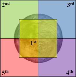
Figure 1. Typical mosaic of five observations taken during each run required for obtaining a complete coverage of one face of Europa. The first piece of the mosaic is overlapping the four others, thus serving as reference to normalize the flux.
Download figure:
Standard image High-resolution imageTable 1. Observation Log
| Time (UT) | Target | I.T. | Airmass | Strehl Mean | Obs. Lon/Lat | S.S.P. Lon/Lat | Φ | P.A. |
|---|---|---|---|---|---|---|---|---|
| 2011 Oct 4th | ||||||||
| 08:01 | Europa 1st mos. piece | 30 s | 1.428 | 13.71 ± 1.38 | 220.1°W; 3.4° | 225.5°W; 3.0° | 5.4° | −20.2° |
| 08:06 | Europa 2nd mos. piece | 30 s | 1.446 | 10.15 ± 0.95 | 220.5°W; 3.4° | 225.8°W; 3.0° | 5.4° | −20.2° |
| 08:11 | Europa 3rd mos. piece | 30 s | 1.465 | 9.74 ± 0.70 | 220.8°W; 3.4° | 226.2°W; 3.0° | 5.4° | −20.2° |
| 08:16 | Europa 4th mos. piece | 30 s | 1.486 | 11.20 ± 0.82 | 221.2°W; 3.4° | 226.5°W; 3.0° | 5.4° | −20.2° |
| 08:21 | Europa 5th mos. piece | 30 s | 1.508 | 11.58 ± 1.29 | 221.5°W; 3.4° | 226.9°W; 3.0° | 5.4° | −20.2° |
| 08:26 | Sky | 30 s | 1.532 | / | / | / | / | / |
| 08:32 | Sky | 30 s | 1.565 | / | / | / | / | / |
| 08:37 | Sky | 30 s | 1.594 | / | / | / | / | / |
| 08:49 | HD 18681 | 20 s | 1.435 | 7.35 ± 1.20 | / | / | / | / |
| 08:54 | Sky | 20 s | 1.454 | / | / | / | / | / |
| 08:58 | HD 18681 | 20 s | 1.474 | 6.88 ± 0.64 | / | / | / | / |
| 2011 Oct 5th | ||||||||
| 05:05 | Europa 1st mos. piece | 30 s | 1.320 | 39.48 ± 1.24 | 309.2°W; 3.4° | 314.4°W; 3.0° | 5.2° | −20.3° |
| 05:10 | Europa 2nd mos. piece | 30 s | 1.310 | 38.61 ± 1.03 | 309.5°W; 3.4° | 314.7°W; 3.0° | 5.2° | −20.3° |
| 05:15 | Europa 3rd mos. piece | 30 s | 1.302 | 37.74 ± 1.22 | 309.9°W; 3.4° | 315.1°W; 3.0° | 5.2° | −20.3° |
| 05:20 | Europa 4th mos. piece | 30 s | 1.294 | 39.39 ± 1.62 | 310.2°W; 3.4° | 315.4°W; 3.0° | 5.2° | −20.3° |
| 05:25 | Europa 5th mos. piece | 30 s | 1.288 | 39.56 ± 0.59 | 310.6°W; 3.4° | 315.8°W; 3.0° | 5.2° | −20.3° |
| 05:30 | Sky | 30 s | 1.282 | / | / | / | / | / |
| 05:40 | Sky | 30 s | 1.273 | / | / | / | / | / |
| 05:45 | Sky | 30 s | 1.270 | / | / | / | / | / |
| 05:55 | HD 18681 | 2 s | 1.263 | 38.88 ± 0.98 | / | / | / | / |
| 05:58 | Sky | 2 s | 1.258 | / | / | / | / | / |
| 06:02 | HD 18681 | 2 s | 1.254 | 39.89 ± 0.99 | / | / | / | / |
| 2011 Oct 21st | ||||||||
| 03:39 | Europa 1st mos. piece | 30 s | 1.342 | 29.14 ± 1.26 | 127.2°W; 3.3° | 128.8°W; 3.0° | 1.8° | −20.8° |
| 03:44 | Europa 2nd mos. piece | 30 s | 1.331 | 30.70 ± 1.35 | 127.5°W; 3.3° | 129.2°W; 3.0° | 1.8° | −20.8° |
| 03:49 | Europa 3rd mos. piece | 30 s | 1.320 | 31.27 ± 1.13 | 127.9°W; 3.3° | 1295°W; 3.0° | 1.8° | −20.8° |
| 03:54 | Europa 4th mos. piece | 30 s | 1.310 | 34.22 ± 1.80 | 128.2°W; 3.3° | 129.9°W; 3.0° | 1.8° | −20.8° |
| 03:59 | Europa 5th mos. piece | 30 s | 1.301 | 32.72 ± 1.27 | 128.6°W; 3.3° | 130.2°W; 3.0° | 1.8° | −20.8° |
| 04:11 | Sky | 30 s | 1.283 | / | / | / | / | / |
| 04:18 | Sky | 30 s | 1.275 | / | / | / | / | / |
| 04:23 | Sky | 30 s | 1.270 | / | / | / | / | / |
| 04:34 | HD 18681 | 2 s | 1.293 | 24.09 ± 1.34 | / | / | / | / |
| 04:38 | Sky | 2 s | 1.286 | / | / | / | / | / |
| 04:42 | HD 18681 | 2 s | 1.280 | 21.41 ± 2.63 | / | / | / | / |
| 2012 Jan 3rd | ||||||||
| 01:39 | Europa 1st mos. piece | 15 s | 1.405 | 30.39 ± 0.72 | 65.8°W; 2.9° | 55.0°W; 3.1° | 10.8° | −22.2° |
| 01:44 | Europa 2nd mos. piece | 15 s | 1.425 | 32.44 ± 0.98 | 66.2°W; 2.9° | 55.4°W; 3.1° | 10.8° | −22.2° |
| 01:50 | Europa 3rd mos. piece | 15 s | 1.447 | 31.72 ± 1.14 | 66.6°W; 2.9° | 55.8°W; 3.1° | 10.8° | −22.2° |
| 01:55 | Europa 4th mos. piece | 15 s | 1.471 | 31.01 ± 2.12 | 67.0°W; 2.9° | 56.2°W; 3.1° | 10.8° | −22.2° |
| 02:01 | Europa 5th mos. piece | 15 s | 1.497 | 28.31 ± 0.66 | 67.4°W; 2.9° | 56.6°W; 3.1° | 10.8° | −22.2° |
| 02:07 | Sky | 15 s | 1.526 | / | / | / | / | / |
| 02:13 | Sky | 15 s | 1.560 | / | / | / | / | / |
| 02:18 | Sky | 15 s | 1.595 | / | / | / | / | / |
| 02:38 | HD 18681 | 3 s | 1.382 | 28.96 ± 1.28 | / | / | / | / |
| 02:41 | Sky | 3 s | 1.391 | / | / | / | / | / |
| 02:43 | HD 18681 | 3 s | 1.401 | 29.93 ± 0.59 | / | / | / | / |
| 2012 Jan 17th | ||||||||
| 01:08 | Europa 1st mos. piece | 30 s | 1.502 | 12.11 ± 2.18 | 42.1°W; 2.9° | 30.7°W; 3.1° | 11.3° | −22.1° |
| 01:13 | Europa 2nd mos. piece | 30 s | 1.527 | 8.89 ± 2.57 | 42.4°W; 2.9° | 31.1°W; 3.1° | 11.3° | −22.1° |
| 01:18 | Europa 3rd mos. piece | 30 s | 1.553 | 4.59 ± 1.95 | 42.8°W; 2.9° | 31.4°W; 3.1° | 11.3° | −22.1° |
| 01:23 | Europa 4th mos. piece | 30 s | 1.581 | 7.91 ± 2.70 | 43.1°W; 2.9° | 31.8°W; 3.1° | 11.3° | −22.1° |
| 01:28 | Europa 5th mos. piece | 30 s | 1.611 | 7.56 ± 1.20 | 43.5°W; 2.9° | 32.1°W; 3.1° | 11.3° | −22.1° |
| 01:33 | Sky | 30 s | 1.646 | / | / | / | / | / |
| 01:44 | Sky | 30 s | 1.727 | / | / | / | / | / |
| 01:50 | Sky | 30 s | 1.775 | / | / | / | / | / |
| 02:04 | HD 18681 | 2 s | 1.463 | 20.26 ± 1.21 | / | / | / | / |
| 02:07 | Sky | 2 s | 1.478 | / | / | / | / | / |
| 02:11 | HD 18681 | 2 s | 1.495 | 22.93 ± 0.36 | / | / | / | / |
Note. Columns from left to right: obervation time, observation target, integration time (I.T.), airmass, Strehl ratio calculated by the SINFONI RTC, apparent planetographic longitude and latitude of the center of Europa seen by the observer, apparent planetographic longitude and latitude of the sun as seen by the observer (S.S.P.), the phase angle (Φ), and the north pole position angle (P.A.). The last four details are provided by NASA JPL Ephemerides (http://ssd.jpl.nasa.gov/).
2.2. Data Reduction
2.2.1. ESO Pipeline
The processing of these complex data involves several steps. The first step uses the standard calibration routines of the ESO SINFONI data-reduction pipeline v2.4.3 and GASGANO. It first corrects all of the raw frames for bad detector cosmetics such as spurious horizontal lines that are created upon readout. The tool also produces all of the basic calibration files: bad pixel masks, master darks, master flats, wavelength solution, and geometric distortion calibration. Unfortunately, because of the instrument data's complex geometry, all of the artifacts were not satisfactorily corrected over the whole wavelength range, leading to about 10 well-identified patches of spurious pixels (a patch consists of between 4 and 8 juxtaposed pixels) for each observation. The final outputs of the ESO pipeline are reconstructed 3D cubes (x, y, λ) in detector count values.
2.2.2. Telluric Correction
The next step of the data-reduction process consists of correcting each pixel for atmospheric absorptions and calibrating the reflectance spectra. The following formula is applied to each cube:
The coefficient  depends on (1) the integration times of Europa and the telluric star
  and
and  , respectively), (2) the angular surface Ωpixel of a pixel (3.65 × 10⁻¹⁵ sr), (3) the apparent magnitude of the Sun seen from Jupiter
  , and (4) the apparent magnitude of the telluric
  . To reduce the noise and obtain more accurate reflectance values, the telluric flux is evaluated over a circle of 11 pixels in radius around the center peak of the point-spread function (PSF). The radius value is visually estimated by studying the aspect of the PSF at 2.4 μm and includes the primary and secondary diffraction lobes. Note that the PSF is better defined at large wavelengths than at small ones. This causes a slight undervaluation of the star flux at small wavelengths, which introduces an overestimate of the reflectance and a slope effect in the correction. This slope effect is minimal for a Strehl value of ∼40% but needs to be corrected for lower values (see Section 3.1).
2.2.3. Mosaic Reconstruction
An important step in the reduction scheme is the reconstruction of the mosaic from the five cubes. The central piece of the mosaic (referred to as central in Figure 1), which has squares of 16 × 16 or more pixels overlapping with the other 4 pieces, is used to normalize the whole mosaic. The flux value over the whole wavelength range (excluding the main atmospheric contamination zone between 1.80 and 1.92 μm) is summed for all of the overlapping pixel squares of the mosaic's eccentric pieces and for the central one, which gives Reccentric and Rcentral, respectively. We then normalized each eccentric piece of the mosaic to the central one by multiplying them by their respective factor  . Values of
  range over the interval [0.90, 1.15], except for one piece taken during the 2012 January 17 run that has a very low Strehl. This piece mostly affects the region of Europa located between 30°S and 15°N in latitude and 355°W and 40°W in longitude. The merging of the five pieces provides a single 3D cube for each night of observation.
2.2.4. Photometric Corrections
Photometric correction is then applied to obtain the geometrically corrected reflectance. We approximate Europa's surface as a Lambertian surface and correct the data cube of each run by the following factor:

where  and SSP are, respectively, the radius of Europa (in pixels) at the time of observation and the distance (in pixels) between the pixel and the sub-solar point. The result is visually convincing until angle values typically ranging between 50° and 60° (Figure 2). For larger angles, the reflectance is larger than 1, which is likely because the Lambertian surface hypothesis is no longer valid. We therefore remove the pixels for incidence >50°, 55°, or 60° depending on the night. Finally, a phase angle effect correction was performed using the phase curve derived in the visible wavelength range from ground-based observations without taking into account the opposition effect (Domingue & Verbiscer 1997). This leads to a maximal correction factor of 1.12.

Figure 2. (Top) Five faces of Europa observed during five runs sorted chronologically. (Bottom) The corresponding SINFONI reflectance maps at 2 μm. Color code goes from violet (minimum reflectance) to red (maximal reflectance). Because of inhomogeneous telluric divisions, scale bars are not equal between observations, and thus are not shown. The suppression of spurious pixels at the edges of every mosaic piece led to partially truncated data. A few small patches corresponding to very locally overvalued or undervalued pixels are still present on each observation, mainly close to truncated parts. Some features, such as craters and dark areas, are clearly identifiable. Regions that are darker in the visible range have a higher reflectance value at 2 μm than the brighter ones.
Download figure:
Standard image High-resolution image2.2.5. 3D Reflectance Cube
One of the major interests of the ESO data set is its potential global spatial coverage. The first step toward obtaining a global reflectance cube is to rotate each observation by Europa's north pole position angle at the time of observation (see the last column of Table 1). The second step then consists of merging the five observations. However, the observations were not taken in the same atmospheric conditions, which leads to images of varying quality as defined by their different Strehl ratio values (Table 1): the highest-quality observation was acquired on 2011 October 05, two good observations were taken on 2011 October 21 and 2012 January 03, and the two observations of 2011 October 04 and 2012 January 17 had an unusually low Strehl ratio. These variable conditions affect the reflectance level and the spectral slope from observation to observation. Hence, an additional normalization procedure prior to the merging step is performed using the best observation (2011 October 05) for reference in terms of reflectance level and spectral slope. Because of the low Strehl ratio of the 2011 October 04 and 2012 January 17 observations, we first apply a two-step reflectance level correction: (i) a ratioed spectrum is derived by dividing the median spectrum of the area overlapping geographically the reference observation to the median spectrum of that same area belonging to the reference observation; (ii) then, all of the pixels of the 2011 October 04 and 2012 January 17 observations are divided by this ratio spectrum. All of the observations are then normalized by adjusting the slope (calculated between 1.70 and 2.20 μm) using the best observation for reference. These normalization processes may generate some slight systematics in the non-reference observations because of the noise and artifacts in the median spectrum of the reference observation; nevertheless, it allows us to significantly reduce the impact of systematics common to all of the observations. The projection of the five observation nights can then be performed. Each night cube is resampled according to an equirectangular projection onto a 360 × 180 pixel matrix. The final product consists of a single 3D reflectance cube that covers about 70% of Europa's surface between −60° and +60° of latitude with a spatial sampling of 35 × 70 km/pixel (i.e., in the theoretical case where the Strehl value reaches 100%), which is comparable to the Galileo NIMS global observations (Carlson et al. 1992, 2005). As a consequence of the variable conditions of observations used to construct this global map, the spectra of the trailing hemisphere are globally of better quality than those of the leading hemisphere, particularly for wavelengths in the 1.7–2.0 μm range and larger than 2.35 μm.
3. MAPS AND SPECTRA
3.1. The 2.00  m Albedo Map

The reflectance map at 2 μm is shown in Figure 3 and compared to the Europa USGS map (USGS Map-a-planet: http://astrogeology.usgs.gov/tools/map). The main geological provinces, as mapped by Doggett et al. (2007, 2009), are also outlined with dark lines. Correlations of the 2 μm map with some of these provinces are clearly visible, as described below. The smallest reflectance values at 2 μm (≤0.08) are found in the Pwyll crater (271°W, −25°N), in the Falga Regio (210°W, 30°N), in an unnamed (and bright in the visible) area in the north of the leading hemisphere centered at (120°W, 30°N), as well as in two undefined areas south of the Annwn Regio (320°W, 20°N) and the Dyfed Regio (260°W, 10°N). The Dyfed Regio and Tara Regio borders are barely visible with medium reflectance values (0.12–0.15). Finally, the highest reflectance values (≥0.16) are observed in two different locations: near the antijovian point (180°W, 0°N) and in a small dark chaos (355°W, 0°N) extending westward of Annwn Regio. Note, however, that the antijovian bright spot can be partly attributed to the accumulation of small approximations (mainly resulting from the telluric division and photometric corrections) during the data reduction process. We will see that most of the albedo variations reported here are correlated to variations of material abundances (Section 5).
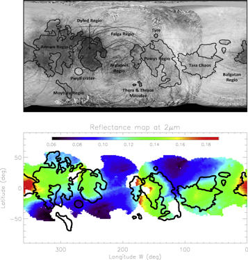
Figure 3. Europa USGS map in the visible wavelength (top) compared to SINFONI-based reflectance map at 2 μm (bottom). Overplotted in black are approximate locations of major geomorphological units identified by Doggett et al. (2009). The maps are displayed in equirectangular projection.
Download figure:
Standard image High-resolution image3.2. Water-ice Maps
As a preliminary investigation of Europa's surface composition, we map the water-ice signatures. Within the SINFONI wavelength range, the absorption at 2 μm is the most appropriate for such an analysis. For each pixel, we divide the median reflectance value over the 1.995–2.005 μm range by the continuum value at 2 μm extrapolated from the slope between 1.745 and 2.235 μm (median values over 20 wavelengths centered at each value; Figure 4). Performing spectral ratios has the advantage of eliminating most of the artifacts observed in the 2 μm reflectance map, although some are still present because of the complex geometry of SINFONI, as previously discussed (see Section 2.2.1). The very typical "bullseye" feature reported in previous global surface composition studies (McEwen 1986; Carlson et al. 2005; Grundy et al. 2007; Brown & Hand 2013) is also visible here on the orbital trailing hemisphere. This feature is well correlated to the non-icy areas and to the dark trailing hemisphere in the visible wavelength range. Other large-scale variations associated with geomorphological units identified by Galileo are also sometimes observed. In spite of residual instrumental artefacts recognizable by localized straight lines and spurious pixels, some features (at SINFONI spatial resolution) such as the Pwyll crater and the Tara Regio are barely resolved as exhibiting values of the spectral parameter (0.38 and 0.40 on their center) significantly different from their surrounding terrains. Large areas with low visible albedo, including the Annwn Regio and Dyfed Regio, are also distinguishable by their low 2 μm signatures.

Figure 4. (Top) Band/continuum at 2 μm used to characterize the water-ice distribution. (Bottom) Band/continuum at 1.65 μm used to characterize the crystallinity of water ice. The maps are displayed in equirectangular projection and black stars represent the areas from which the spectra are extracted for further analyses in Figures 5 and 8.
Download figure:
Standard image High-resolution imageWe produced a similar global map for the absorption at 1.65 μm, which is characteristic of crystalline water ice (Figure 4). This feature is very well defined in the data set due to the high spectral resolution of the SINFONI instrument. A specific spectral criteria index is derived by dividing the median reflectance in the 1.647–1.653 μm range by the corresponding values of the continuum. A straight-line segment from the absorption's left wing (1.61–1.62 μm) and right wing (1.69–1.70 μm) was used to approximate the continuum line. The spectral criteria is lower than 1 for all pixels, indicating that the 1.65 μm feature is present in all of the SINFONI spectra. The spatial variations are well correlated at first order with the distribution of the 2 μm criteria: the stronger the 2 μm water-ice band is, the stronger the crystalline feature is. The surface of the leading hemisphere exhibits much stronger signatures than the trailing one. The smallest values (≤0.85) derived in the northern hemisphere of the leading side presume the presence of crystalline water in large abundance. As for the absorption at 2 μm, the map highlights correlations with some major geomorphological units: the Powys Regio and Tara Regio located in the leading hemisphere have slightly higher values than their surrounding areas, while the center of the Pwyll crater exhibits a smaller value (∼0.90) than its surroundings. The area with the weakest absorption is actually well centered on the trailing apex and has an almost perfect ellipsoidal shape. Of special interest is the dependence of the value on latitude in the trailing hemisphere: for a given longitude, the absorption increases with latitude, which is consistent with the decreasing implantation of exogenous sulfur flux and the precipitation of energetic electrons with latitude (Paranicas et al. 2001; Hendrix et al. 2011; Patterson et al. 2012; Dalton et al. 2013).
3.3. Spectra of Different Region of Interests (ROIs)
3.3.1. Global Comparison
Spectral features significantly depend on location. Examples are shown in Figure 5. Spectra are extracted from four regions of interest and are well representative of the spectral diversity of Europa in the NIR wavelength range: (1) leading hemisphere at 120°W, 30°N in the bright icy area in the visible, (2) Dyfed Regio in the trailing hemisphere, which exhibits a low albedo in the visible wavelengths range, (3) a transition zone at (195°W, 0°N) close to antijovian point, and (4) Tara Regio.
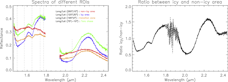
Figure 5. (Left) Representative reflectance spectra from the surface of Europa corresponding to the non-icy area of the trailing hemisphere (red), the icy area of the leading hemisphere (blue), the transition between these two hemispheres (yellow), and the Tara chaos (green; see black stars for their location in Figure 4). Dotted lines highlight the different spectral features observed in each or some of these spectra. Atmospheric absorptions making the spectra noisy between 1.80 and 1.92 μm, and data in this wavelength range have been removed for clarity. (Right) Ratio between icy and non-icy spectra, with the 1.80–1.92 μm wavelength range represented by the dotted line. The general aspect is characteristic of water ice with a positive slope. No other spectral signature is identified.
Download figure:
Standard image High-resolution imageOverall, the spectral features are fairly consistent with previous NIMS and ground-based observations (Carlson et al. 1999b, 2005; Dalton 2007; Brown & Hand 2013): the leading hemisphere spectra are dominated by well-defined and strong water-ice absorptions, while the trailing hemisphere spectra exhibit distorted and asymmetric water-ice absorptions. Between these two end-members, the spectral features vary gently from place to place. Of special interest is the weak bump at ∼2 μm leading to an absorption feature at ∼2.07 μm which is visible for the spectrum extracted from Dyfed Regio. This feature was first highlighted by Brown & Hand (2013) and interpreted as an absorption feature from magnesium sulfate MgSO4.7(H2O) (epsomite). In order to emphasize this feature, we attempted to perform a spectral ratio by dividing this spectrum by the icy one lacking this feature. However, when making the ratio, this absorption remains invisible because of its weakness compared to water-ice absorptions, which are predominant (Figure 5). Another feature present in all spectra is a shoulder at 1.73–1.74 μm that is sometimes associated with very weak absorption at 1.77–1.78 μm. This feature was also clearly observed in the NIMS and Keck spectra (McCord et al. 1998b; Brown & Hand 2013). Orlando et al. (2005) associated this feature with small cations such as Na+ and Mg2+ in brines, while Dalton et al. (2005) highlighted its spectral coherence with mirabilite (Na2SO4.10(H2O)) and Mg-sulfate dodecahydrate (MgSO4.12(H2O)). Nevertheless, this feature attracted little attention. Given the lack of clear and distinct absorption of a non-icy component, we will see further in this section that these small shoulders are essential to better constrain the nature of the hydrates responsible for the distortion of the water-ice bands.
3.3.2. Crystalline Water Ice
The four representative spectra reveal clear minima at 1.57 and 1.65 μm. The combination of these two strong signatures provides evidence for the presence of crystalline water ice on Europa's surface, as amorphous water ice does not exhibit such strong absorptions (Mastrapa et al. 2008). These absorptions are of special interest because their position are shifted with temperature, and thus can be used as a temperature proxy (Mastrapa et al. 2008). The most reliable value of the surface temperature should be given by the "pure icy" spectrum extracted from the leading hemisphere, which is considered to be less affected by radiation (Pospieszalska & Johnson 1989; Paranicas et al. 2001; Patterson et al. 2012). This radiation could indeed significantly modify the physical properties of the water ice and produce a variation of the 1.65 μm band profile and position (Leto et al. 2005). To increase the S/N, we calculated an average spectrum from a square of 11 × 11 pixels centered on the pixel (120°W; 30°N) representing the icy area in Figure 4, and then resampled the spectrum over 20 wavelengths. The spectral minimum is found to be at 1.650 ± 0.003 μm (Figure 6), which is consistent with the results of Dalton et al. (2012) from low-noise Galileo NIMS observations of the mean temperature. It corresponds to a temperature close to 120 K according to Mastrapa et al. (2008). This temperature is well representative of the mean temperature of the leading hemisphere because more than 97% of its pixels have a spectral minimum in the range λ = 1.649–1.652 μm, which corresponds to T = 110–130 K according to Mastrapa et al. (2008). Moreover, 33% of pixels have a minimum at λ = 1.650 μm, and this value is in the range of daytime temperatures obtained from the Galileo photopolarimeter-radiometer (Spencer et al. 1999; Rathbun et al. 2010).

Figure 6. Enlargement on the water-ice crystalline absorption band at 1.65 μm of (top) a pixel in the icy area (120°, 30°) and (bottom) a pixel in the non-icy area (260°, 10°). Left: data spectra in black and two laboratory reflectance spectra of 120 K crystalline and amorphous water ice. Right: close zooms on 1.65 μm absorption (data in black, smooth in red) compared to pure water-ice spectra of various temperatures (Mastrapa et al. 2008). For the smoothed icy spectrum, we obtain a spectral minimum at 1.6500 μm (black dotted line) corresponding to a temperature close to 120 K (green dashed line). This temperature is very similar to those derived from previous studies (Spencer et al. 1999; Rathbun et al. 2010). The smoothed, non-icy spectrum has a spectral minimum shifted to 1.6545 μm (black dotted line) leading to an unrealistic, very low temperature. This spectrum is poorly suited to temperature sensing due to the nature of the continuum non-icy components that shift the position of the 1.65 μm band.
Download figure:
Standard image High-resolution image3.3.3. Additional Feature: 1.73 Slope Break

As mentioned previously, a second subtle feature is present on every spectrum: a slope break at 1.73–1.74 μm, sometimes with a very weak absorption at 1.77–1.78 μm. The mixture of Mg-sulfate salts with water ice and sulfuric acid hydrate typically used in previously published spectral modeling of Europa's surface cannot reproduce this feature (Figure 7). The sodium sulfate mirabilite (Na2SO4.10(H2O)) was also initially considered as a potential candidate to explain this feature, but the absence of other mirabilite signatures that should be seen in the data led to the rejection of this mineral (Dalton 2007; Brown & Hand 2013).
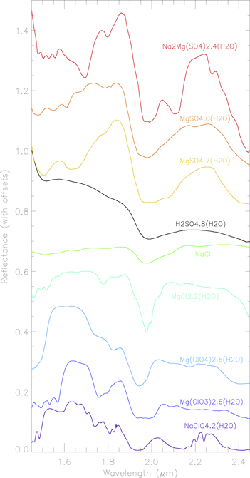
Figure 7. Some laboratory reflectance spectra used for the linear spectral modeling coming from three major sources (Dalton 2007; Dalton & Pitman 2012; Hanley et al. 2014). Purple to green: chlorine salts at 80 K. Black: sulfuric acid hydrates at 140 K. Yellow to red: Mg-sulfate salts at 120 K. Bottom to top, the curves are positively offset by +0.0, +0.1, +0.2, +0.3, +0.4, +0.55, +0.7, +0.8, and +0.9.
Download figure:
Standard image High-resolution imageWe started considering a very large variety of potential minerals that could help in reproducing this feature. The recent study of Hanley et al. (2014) presents cryogenic reflectance spectra of many chlorine salts. Some of them exhibit a clear shoulder at 1.70–1.75 μm that is likely due to the hydrated phases of these salts. This feature is associated with asymmetric and distorted water-ice absorption presenting a shifted spectral minimum at 1.93–1.97 μm (Figure 7). Such spectral characteristics are consistent with the observations in SINFONI spectra of the non-icy area. In this respect, we will further consider this salt species as a potential candidate to reproduce some of the spectral properties of Europa surface (see Section 4.3).
4. SPECTRAL MODELING
4.1. Linear Mixture Model
In order to refine the surface composition and its variations at the surface of Europa, SINFONI spectra are resolved into materials via a linear deconvolution technique. Linear deconvolution is based on the principle that the spectrum is a linear combination of the spectra of the different species composing the icy and non-icy surfaces of the satellite in proportion to their abundance. The unmixing technique uses a library of end-member laboratory spectra to perform an iterative best fit of the spectra. Each modeled spectrum  is thus calculated as

where  is the number of reference laboratory spectra
  ) used and
  i is their abundance. Since slight geometric and photometric uncertainties may affect the spectral slope, one additional free parameter S is used to adjust the continuum spectral slope. The downhill simplex method we used (Nelder & Mead 1965) proceeds to successive calculations, varying the abundances of each end-member and the slope value until a best fit is achieved. The quality of the fit is evaluated by a visual, qualitative comparison of the model and measured spectra, and is quantified by the chi-squared value
  . To calculate
  , we excluded the 1.79–1.94 μm wavelength range due to spurious values produced by residual telluric lines. Conversely, we doubled the weight for the wavelength ranges 1.56–1.67 μm and 1.97–2.10 μm to better reproduce the crystalline water-ice absorption feature and the absorption at ∼2.07 μm on the trailing side spectra (Figure 5 and discussed in Section 3.3.1).
Linear unmixing is a first-order approach justified by the fact that the large pixel scale of SINFONI unavoidably results in the spatial (hence linear) mixing of various surface components. The presence of several components within the SINFONI pixel scale is confirmed based on higher-resolution SSI and NIMS observations. However, as we will discuss later, residuals from the model may be due in part to intimate mixing which is not accounted for in a linear approach.
4.2. Cryogenic Library
Initial examinations of the spectra show general matches to the laboratory spectra of end-members already used in previous studies, namely, water ice (both crystalline and amorphous water ice) mixed with non-icy components (possible sulfate minerals and/or sulfuric acid). For sulfate salts, the spectra of bloedite, hexahydrite, and epsomite were measured at 120 K by Dalton & Pitman (2012) and sulfuric acid hydrate is the octohydrate measured at ∼140 K originating from Carlson et al. (1999b). As discussed in Section 3.3.3, some subtle features in the 1.68–1.80 μm wavelength range could indicate the presence of chlorine salts. Various phases were considered with the cryogenic spectra at 80 K all coming from Hanley et al. (2014): the chloride MgCl2.2(H2O), the chlorate Mg(ClO3)2.6(H2O), and the perchlorate Mg(ClO4)2.6(H2O). The non-icy reference spectra we used as end-members are shown in Figure 7. The temperature of their acquisition and the size of the grains (when specified) are reported in Table 2.
Table 2. Characteristics of Non-ice Laboratory Reflectance Spectra Tested for Modeling
| Chemical Formula | References | Temperature | Grain Size |
|---|---|---|---|
| H2SO4.8(H2O) | Carlson et al. (1999b) | 140 K | ∼50 μm |
| MgCl2.2(H2O) | Hanley et al. (2014) | 80 K | / |
| MgCl2.4(H2O) | Hanley et al. (2014) | 80 K | / |
| MgCl2.6(H2O) | Hanley et al. (2014) | 80 K | / |
| Mg(ClO3)2.6(H2O) | Hanley et al. (2014) | 80 K | / |
| Mg(ClO4)2.6(H2O) | Hanley et al. (2014) | 80 K | / |
| MgSO4 brine | Dalton et al. (2005) | 100 K | 50–150 μm |
| MgSO4.6(H2O) | Dalton & Pitman (2012) | 120 K | 100–200 μm |
| MgSO4.7(H2O) | Dalton & Pitman (2012) | 120 K | 100–200 μm |
| MgSO4.12(H2O) | Dalton et al. (2005) | 100 K | ∼50 μm |
| Na2CO3.10(H2O) | McCord et al. (2001) | ∼100 K | 355–500 μm |
| Na2Mg(SO4)2.4(H2O) | Dalton & Pitman (2012) | 120 K | 125–150 μm |
| NaCl | Hanley et al. (2014) | 80 K | / |
| NaClO4 | Hanley et al. (2014) | 80 K | / |
| NaClO4.2(H2O) | Hanley et al. (2014) | 80 K | / |
| Na2SO4.10(H2O) | Dalton et al. (2005) | 100 K | 100–150 μm |
Note. Columns from left to right: chemical formula, reference paper, temperature, and grain size. In bold are the spectra represented in Figure 7.
Download table as: ASCIITypeset image
Finally, the reflectance spectra of amorphous and crystalline water ices at 120 K were derived from the Shkuratov radiative transfer model (Shkuratov et al. 1999; Poulet et al. 2002) using the optical constants of both types of water ices provided by Mastrapa et al. (2008) and by the GhoSST online database (http://ghosst.osug.fr). We generated reflectance spectra for grain sizes d = 5 μm, 25 μm, 200 μm, and 1 mm.
4.3. Results
We first applied the linear mixture model to the spectra representative of the spectral diversity of Europa (Figure 4). We adopt a tailored, iterative approach to unmixing, starting with a small set of end-members and then increasing to a larger set of end-members to improve the fit (Figure 8). This step is crucial to determine which components will be required for subsequent modeling of the complete data set (see Section 5). Based on previous modeling, the presence of sulfuric acid hydrate mixed with water ice (both amorphous and crystalline) is assumed to be mandatory, so that the following eight end-members, i.e., four crystalline water-ice spectra (5 μm, 25 μm, 200 μm, 1 mm), three amorphous water-ice spectra (25 μm, 200 μm, 1 mm), and one sulfuric acid hydrate spectrum, are by default included in the spectral library.
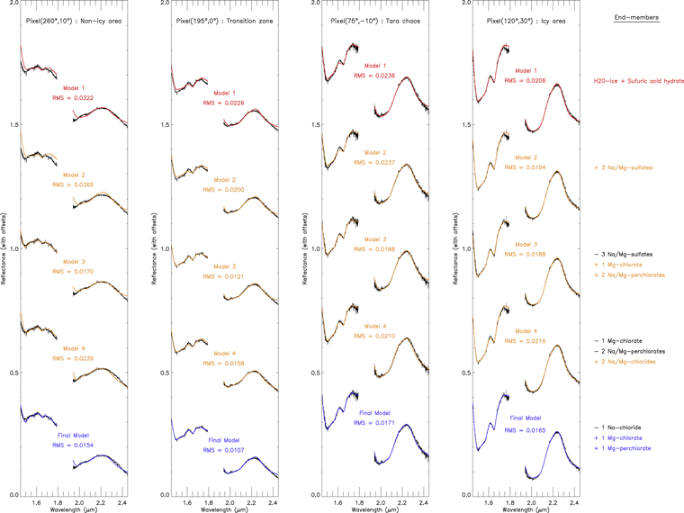
Figure 8. Single pixel raw spectra (black) with their associated model (red, orange, or blue) obtained by using different end-members of the cryogenic library previously presented in Figure 7. Each model has a corresponding rms. From top to bottom for every column, the spectra are, respectively, offset by +1.4, +1.05, +0.70, +0.35, and +0.0. They correspond to the best fit obtained with (1) H2O ice + sulfuric acid hydrate, (2) H2O ice + sulfuric acid hydrate + the three Mg/Na-sulfate salts, (3) H2O ice + sulfuric acid hydrate + the Mg-chlorite ( ) and the two Mg/Na-perchlorates (
 ), (4) H2O ice + sulfuric acid hydrate + the two Mg/Na-chlorides (Cl−), and (5) H2O ice + sulfuric acid hydrate + the three Mg-chlorines. In each of these cases, the best-modeled spectra (represented in blue) are obtained by adding the three Mg-chlorines of our library to H2O ice and sulfuric acid: chloride MgCl2.2(H2O), chlorate Mg(ClO3)4.6(H2O), and perchlorate Mg(ClO4)4.6(H2O). No improvement is noted when using our whole library.
Download figure:
Standard image High-resolution imageMixtures of these eight end-members provide satisfactory fits (referred to as model 1 of Figure 8) of the leading icy area and Tara Regio spectra, while some clear discrepancies are visible for the less icy spectra (named "non-icy" and "transition zone" in Figures 5 and 8). These discrepancies are notably strong for "ice-related" absorption features at 1.5 and 1.65 μm, as well as at ∼1.75 μm and the ∼2 μm bump. These discrepancies decrease gradually as spectra become icier, but even for the "pure" icy spectrum, a small but still significant difference given the high S/N of the data persists in the 1.73–1.80 μm range that cannot be attributed to instrument artefacts or residuals from the data-reduction process.
A second iteration in the optimization procedure consists of adding different sulfate salts such as bloedite, hexahydrate, and epsomite (referred to as model 2 of Figure 8). Surprisingly, the addition of these end-members does not improve the fits, especially for the non-icy one which shows a frank overestimation between 1.69 and 1.8 μm. This result challenges the presence of Mg/Na-sulfate salts on Europa's surface. A third test is applied by replacing Mg/Na-sulfate salts by Mg-chlorate (Mg(ClO3)2.6(H2O)) and Mg/Na-perchlorates (Mg(ClO4)2.6(H2O), NaClO4.2(H2O)). Modeled spectra (referred to as model 3 of Figure 8) are clearly improved, especially for the non-icy and the transition zone pixels. As shown in Figure 4, water-ice absorption features at 1.50 and 1.65 μm, as well as the small shoulder at 2.07 μm associated with the ∼2 μm bump, are much better reproduced. In addition, reflectance is no longer overestimated in the 1.69–1.80 μm range, which further emphasizes the presence of chlorine species. We then performed additional tests by replacing the perchlorates used in model 3 by chlorides such as NaCl and MgCl2.2(H2O) (referred to as model 4 of Figure 8). Best-fit modeled spectra are globally less convincing than those of the previous test, with the exception of the 1.73 μm slope break and the slight absorption at 1.77 μm visible in the non-icy spectra which are well reproduced. This results from the spectral contribution of MgCl2.2(H2O), which has an absorption feature in this wavelength range. For this reason, we will keep this end-member for the next modeling. We also evaluated the presence of Na-chloride and Na-perchlorate instead of Mg-bearing ones (not shown here). Once again, the modeled spectra are worse than those obtained with model 3, as confirmed by larger rms and sometimes by a weak but distinct absorption at ∼2.24 μm resulting from the Na-perchlorate. Such a feature is not present in the data, likely ruling out the presence of this mineral on the surface of Europa.
Several other combinations using the different species listed in Table 2 were tested but the best fits (referred to as the final model of Figure 8) were eventually obtained by using only Mg-bearing chlorinated salts (the chloride MgCl2.2(H2O), the chlorate Mg(ClO3)2.6(H2O), and the perchlorate Mg(ClO4)2.6(H2O)) in addition to the default end-members listed previously. Fits are actually excellent for the Tara Regio and the leading hemisphere icy area. The non-icy spectrum with its bump at ∼2 μm is very well reproduced. The discrepancies that are still present in the non-icy spectra are the position and the band depth of the 1.50 and 1.94 μm absorptions and the slightly curved shape of the model in the range 2.25–2.45 μm. These discrepancies could result from a limited range of end-members and a degree of hydration or grain size effect. Radiation could also significantly modify these features (Leto et al. 2005). Using water-ice spectra at 80 and 100 K instead of at 120 K produces only minor variations in terms of abundance (<8%). A last best-fit test was performed using the complete library, but the improvements compared to the previous modeling are not significant. We conclude that the surface of Europa as observed by SINFONI can be correctly modeled with the three following families of species: crystalline and amorphous water ices, sulfuric acid hydrate, and Mg-chlorinated salts; meanwhile, sulfate salts are not required.
5. GLOBAL MAPS
Before performing linear modeling on the 3D data cube using all of the icy and mineral species, the spectra were smoothed over 10 wavelengths to increase the S/N and to diminish the computing time given the large number of spectra. The spectral smoothing leads to a substantial improvement of the rms for some areas (e.g., for Tara Regio rms = 0.012 in comparison to rms = 0.017 before smoothing) without missing any subtle spectral signature. Slight differences in terms of the absolute abundance value of the sulfuric acid hydrate and of water ice with a large grain size before and after spectral smoothing are found, but they are not significant (<5%–10%). After visual inspection of several tens of modeled spectra, we selected the rms = 0.02 as a threshold below which the fits are assumed to be satisfactory. As shown in Figure 9, the spectra are well reproduced, except at the antijovian point and in the northern part of the icy area. These high rms values in the range of 0.02–0.03 are due to a misfit in the 1.97–2.10 μm range where the weight of the spectral elements is doubled (see Section 4.1). A nonlinear mixture model could help to improve the fits, but the linear mixing provides overall extremely good fits and has the advantage of not requiring optical constants that are lacking for some species (especially chlorine and sulfate salts). In the following, we present the spatial distribution of each species.
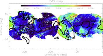
Figure 9. χ2 map of linear spectral modeling best fits. 93% of the spectra have χ2 ≤ 0.015.
Download figure:
Standard image High-resolution image5.1. Sulfuric Acid Hydrate
As expected, the sulfuric acid hydrate is mainly present on the trailing side (Figure 10) with a maximum concentration of ∼65% near the trailing apex (270°W, 0°N). This abundance is lower than the ∼90% reported in Carlson et al. (2005) and Brown & Hand (2013). The largest concentrations are consistent with the trailing apex (0°W, 270°N) and are not correlated with geomorphological units. In the leading hemisphere, the spatial distribution is also uneven and uncorrelated with geomorphology. The range of values goes from 0% to 10% in the bright, icy area to 30%–40% in the eastern part of the Tara Regio and in the Balgatan Regio (30°W, −50°N). In both hemispheres, the concentration of sulfuric acid hydrate decreases with latitude and is anti-correlated with the water-ice band depth maps previously presented (Figure 4). A first attempt at estimating the uncertainty due to the measurement of the abundance is to compare the derived values for regions that were observed twice. The equatorial region of longitude 175°W was observed during the 2011 October 04 and 2011 October 21 runs. Differences of ∼20%, ∼25%, and ∼10% for sulfuric acid hydrate, water ices, and chlorine salts, respectively, were derived between the best fits of the two juxtaposed regions observed during two different nights. As mentioned in the description of the 2 μm reflectance map (see Section 3.1), this discrepancy is due to an accumulation of small approximations before reconstructing the global 3D reflectance cube and leads to an error of ∼25% on the reflectance level. Additional tests that take into account this uncertainty have been performed on the reference spectra presented in Figure 5 and, as expected, we found very similar abundance variations to those mentioned previously in this section. Thus, the difference of 25% is the largest derived for all of the end-members, and it corresponds to the maximal error on the abundance estimate.
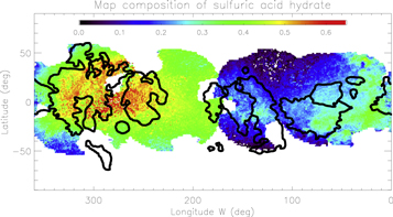
Figure 10. Spatial distribution of sulfuric acid hydrate. The highest concentrations (up to 65%) are observed on the trailing hemisphere apex. The distribution is also uneven in the leading hemisphere with no clear spatial correlation with geomorphological units.
Download figure:
Standard image High-resolution image5.2. Water Ices
5.2.1. Amorphous Water Ice
The amorphous water-ice composition map using the three different grain sizes is exclusively dominated by the leading/trailing effects (Figure 11(a)). The lowest concentrations are located near the trailing apex with an average value lower than 5%, while the highest values reach 40% at high latitudes in the south of the leading hemisphere. Geomorphological units are not distinguishable.

Figure 11. Spatial distributions of (a) amorphous water ice (all sizes), (b) crystalline water ice (all sizes), (c) 1 mm grain crystalline water ice, and (d) 5 μm grain crystalline water ice. Very localized high concentrations of 5 μm grains are spatially correlated with "darker" terrains (in the visible range). The 1 mm grain distribution does not show any spatial coherence with the apex of the trailing hemisphere (see text).
Download figure:
Standard image High-resolution imageWhen analyzing the spatial distribution as a function of the three different grain sizes used in the modeling, we observe that the largest grain size (1 mm) has a very low abundance below the detection threshold, except for a spot of ∼20% in the south–west of the trailing hemisphere (340°W, −40°N). This area is spatially correlated with the area that exhibits the strongest 2 μm signature of the trailing hemisphere (Figure 4). The 200 μm sized grains are present only on the leading side, particularly in the bright, icy area and in the terrains surrounding the Tara Regio with maximum concentrations of 15%–20%. The spatial distribution of the 25 μm grains is actually very similar to the overall amorphous water ice, with concentrations slightly above 35% for some pixels in the southern part of the Powys Regio. This abundance, which is approximately twice as large as the largest abundance of 200 μm, combined with the quasi-absence of 1 mm grain size, therefore indicates a surface that is globally dominated by small grains.
5.2.2. Crystalline Water Ice
Contrary to the case of amorphous ice, the spatial distribution of the crystalline water ice (Figure 11(b)) is much more related to the geomorphological units. Annwn and Dyfed Regio are depleted in water ice (<15% on average) in comparison to their surrounding terrains, while the abundance goes up to 65% for the northern bright, icy area with an average of 40%–55% in the leading hemisphere. The Pwyll crater presents a mean abundance that is three times larger than the surrounding terrains (32% versus 10%). Overall, the global distribution is well consistent with the map at 1.65 μm previously derived to map the crystallinity character of water ice (Figure 4).
The spatial distribution of the different grain sizes has also been studied. As shown in Figure 11(c), the 1 mm grains are exclusively found in the trailing hemisphere with a 15%–30% abundance localized in Argadnel and Falga Regio where large lineae (e.g., Cadmus, Minos, etc.) are present (Doggett et al. 2009). The distribution of 200 μm grains is concentrated only in the northern bright, ice-rich triangle of the leading hemisphere with a maximum abundance of 30%. The 25 μm grains are mainly found in the leading hemisphere. Thus, the addition of the abundances of the 25 and 200 μm grains reproduces very well the distribution of the leading hemisphere and explains well the distribution of the trailing regions. It supports the fact that the Jovian moon surface is globally dominated by water-ice grains with sizes in the range 25–200 μm. The smallest grain size (5 μm) used in the modeling is detected with confidence in the unnamed dark chaos extending westward of the Annwn Regio (Figure 11(d)), which has also been identified as the spot with the largest reflectance at 2 μm (Figure 3). This area of very small grains does not seem to be correlated with exogenous processes. This raises questions about its origin and the role of endogenous processes in the composition of the surface of Europa.
5.3. Mg-bearing Chlorinated Salts
As for the sulfuric acid hydrate, chlorine salts (bearing the Mg cation here) are significantly more abundant in the trailing hemisphere than in the leading one (Figure 12(a)). However, unlike the former, their distribution is correlated with several geomorphological units, with regional enhancements of up to 35% corresponding to, e.g., the Dyfed Regio and the small dark chaos extending westward of the Annwn Regio. Significant concentrations of 20%–30% are also found in the Annwn Regio. In the leading hemisphere, abundances as low as 5% are observed in the icy areas, while the Tara Regio and Powys Regio locally exhibit higher abundances, sometimes exceeding 20%.
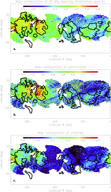
Figure 12. Spatial distributions of (a) all Mg-bearing chlorinated salts, (b) Mg-perchlorate Mg(ClO4)2.6(H2O), and (c) Mg-chloride MgCl2.2(H2O). While the Mg-chloride distribution is correlated with dark terrains with abundances reaching 25% on the chaos westward of the Annwn Regio, the perchlorate map exhibits a significant concentration centered on the apex of the trailing hemisphere (approximately 15%).
Download figure:
Standard image High-resolution image
Among this family, the Mg-perchlorate distribution (Figure 12(b)) shows a strong dichotomy between the two hemispheres as the largest abundances (∼17%) are approximately centered on the trailing apex where the surface is most subject to exogenous ionic and electronic implantation (Patterson et al. 2012; Cassidy et al. 2013). The second compound, Mg-chlorate, is low in abundance (≤12%), and no clear link to geomorphology can really be argued. This phase is at the limit of the detection threshold, although its addition to the spectral library still improves the quality of the fit, especially in the trailing hemisphere. Finally, Mg-chloride is the most abundant of the three chlorine salts used in the modeling, and its distribution, as shown in Figure 12(c), is globally similar to the global distribution of the chlorine species. An abundance peak is observed in the small, dark chaos at 350°W where a spot of 5 μm grain of crystalline water ice was also identified, as well as in the Dyfed Regio and Tara Regio. This unexpected spatial distribution linked with the geomorphology challenges the hypothesis on the fully exogenous origin of the non-H2O species present on the surface of the satellite. In the following section, we address in greater detail the origin and evolution of the species against exogenic and endogenic processes.
6. DISCUSSION
6.1. The Mg-bearing Chlorinated Species Hypothesis
The spectral modeling highlights the need for (Mg-bearing) chlorinated species to better reproduce the NIR spectral signatures on a global scale rather than Na/Mg-sulfates (Figure 8). All of the spectral characteristics not associated with H2O ice or sulfuric acid hydrate absorptions, such as the slope break ∼1.73 μm and the small shoulder at ∼2.07 μm, can be explained by the spectral features of Mg-bearing chlorinated species. The ∼2 μm distorted signature is also very well fit. Nevertheless, the presence of the three chlorine species used in this work cannot be definitely asserted as their spectral effects are subtle and bear similarities to other hydrated chlorinated species. The temperature of 80 K at which the laboratory spectra were acquired is not exactly representative of Europa's surface temperature, and their concentrations (≤35% in total) still remain minor compared to the H2O ice and sulfuric acid hydrate. Using a spectral library at temperatures more similar to those of Europa could then modify the derived abundances of these species. Thus, additional high spectral resolution campaigns in different wavelength ranges (<1.5 μm) combined with a cryogenic library at temperatures >80 K would be helpful to better constrain the abundances of the Cl-bearing salts and to confirm or disprove their presence on the surface of the satellite.
Most studies have considered that the dark, non-ice component observed principally on the trailing hemisphere is related to Mg-sulfate species. This predominance of sulfates compared to chlorines was first attributed to a very low cosmic abundance ratio Cl/S (Kargel 1991) and supported by theoretical and experimental estimates of Europa's ocean composition based on the aqueous alteration of a CM chondrite meteorite (Kargel et al. 2000; Fanale et al. 2001; Zolotov & Kargel 2009). However, chlorine ions have been detected in the plasma torus (Küppers & Schneider 2000; Feldman et al. 2001), and water-rock cycling at the silicate seafloor could lead to a chloride-rich ocean (Glein & Shock 2010). While some geochemical models predict that Europa's initial chondritic composition should lead to a chlorine-poor ocean, recent theoretical models of the subglacial ocean of Enceladus, the Saturnian icy moon comparable to Europa, predict a Cl-rich ocean (Zolotov 2007; Glein et al. 2015). The chlorine salts hypothesis was also recently proposed to explain the color of the Europan surface in the visible and NIR wavelength ranges (Fischer et al. 2015; Hand & Carlson 2015).
Concerning the magnesium, the absence of magnesium ions in the Ionian plasma torus and the very low contribution from micrometeoroid bombardment suggests an endogenous origin for this chemical element (Carlson et al. 2009). Its predominance on the surface compared to Na/K-bearing species may be explained by a sputtering erosion rate that is much less efficient for Mg than for Na and K (Horst & Brown 2013), as has been experimentally demonstrated for sulfate salts (McCord et al. 2001). Finally, Brown & Hand (2013) also hypothesized that Mg should primarily be in the form of MgCl2 before being irradiated on the surface.
6.2. Abundance and Grain Size of Water Ice
Our study confirms the high predominance of H2O ice and sulfuric acid hydrate, as they represent overall more than 80% of the surface abundance on average. These two components are well anti-correlated: while the overall abundance of H2O ice rises to almost 90% on the bright (visible) area of the leading northern hemisphere, the sulfuric abundance increases gradually toward the trailing hemisphere until reaching approximately 65% on the orbital trailing apex, which corresponds to the highest magnetospheric bombardment intensity and the center of the sulfur flux (Paranicas et al. 2001; Hendrix et al. 2011; Dalton et al. 2013). However, as previously mentioned, the abundance is ∼30% lower than those obtained by Hand & Brown (2013) and Carlson et al. (2005) from nonlinear modeling. This difference could be due to the use of a linear versus a nonlinear approach. It is important to note that the 1.65 μm band is much more pronounced in our high spectral resolution data and cannot be well reproduced by less than 15% of water ice (Figure 8). The spatial blurring induced by our moderate Strehl ratios should not induce contamination of the 1.65 μm band within the sulfuric unit by neighboring H2O-rich regions, given the large size of the observed unit.
Most of the spectra can be correctly fit only using the 25 and 200 μm grain sizes. This is consistent with many previous studies (Calvin et al. 1995; Hansen & McCord 2004; Dalton et al. 2012), but no clear relationship between the grain sizes and exogenous processes has been identified, contrary to studies based on very localized Galileo NIMS observations (Dalton et al. 2012; Cassidy et al. 2013). The distributions of larger grains, such as 200 μm and 1 mm (Figure 11(c)), do not show any spatial coherence with the apex of the trailing hemisphere, while the 5 μm crystalline ice distribution also does not look to be controlled by the intensity of the bombardment (Figure 11(d)). This difference suggests that exogenous processes are not the only explanation for the H2O grain size distribution.
6.3. Crystallinity of Water Ice
According to a study based on the 3.1 μm water absorption, H2O ice on Europa is presumed to be mainly amorphous (Hansen & McCord 2004). It is intended that the 3.1 μm Fresnel reflection peak provide major constraints on the nature, whether crystalline or amorphous, of the water ice. However, the 1.65 μm absorption band has also been proven capable of discriminating between the two types of water ice (Schmitt et al. 1998; Mastrapa et al. 2008). Thanks to the high spectral resolution of SINFONI, a detailed study of this absorption has been carried out. Figure 6 clearly highlights that the depth and the position of this absorption cannot be reproduced by amorphous ice alone, both for the leading and trailing hemispheres. The spectral modeling on the global scale also shows the slight predominance of crystalline H2O ice with the ratio of amorphous/crystalline = 0.57 ± 0.25 on average. This result is not inconsistent with the former study based on the 3.1 μm Fresnel. Indeed, it suggests that a positive vertical crystallinity gradient exists in the ice slab covering the surface, as already proposed by Hansen & McCord (2004). This could provide useful hints for reinvestigating the balance between the disruption of crystalline ice by irradiation and crystallization by heating. The surface temperature of Europa being in the range 110–130 K suggests that the crystallization of impure amorphous ice should occur in less than 10 years (Kouchi et al. 1994; Jenniskens et al. 1998; Hansen & McCord 2004; Mastrapa et al. 2013), while the amorphization time is expected to be about 0.6 year for the ion flux Φ = 107 cm2 s−1 corresponding to the trailing apex (Fama et al. 2010).
The large predominance of sulfuric acid hydrate on the trailing hemisphere makes interpretations tricky for any process that could control the nature of the water ice in this hemisphere. However, it is worth noting that the crystalline spots detected at high latitude in this hemisphere (Figures 11(b), (c)) may be explained by the lower efficiency of the radiation-based amorphization at these high latitudes. While both types of water ices are present in the leading hemisphere, significant variations of their relative concentration are nevertheless observed. The relatively high abundance of crystalline ice in the triangular bright, icy area is surprising. It could correspond to a relatively warm formation environment, possibly linked to thermal convection in the ice shell. Melt-through events on Europa due to tidal stress are indeed expected to lead to warmer areas (Greenberg et al. 1998; O'Brien et al. 2002). The increase of amorphous ice concentration in the high latitudes of this hemisphere could indicate a specific source of amorphous ice. Condensation of water vapor near the pole has already been proposed (Hansen & McCord 2004). However, better coverage of the very high latitudes is still required before we can confirm this observation. A very specific and unique concentration of small grain sized crystalline ice is also observed in the chaos located close to the meridian. This could again imply a warm environment, possibly linked to an endogenic process as the chloride salts also exhibit an enhancement of their abundance (see the next section).
6.4. Role of Exogenous and Endogenous Processes
In agreement with previous studies, the origin of sulfuric acid is proposed to be exogenous, precisely Iogenic, as its distribution is perfectly correlated to the Iogenic sulfur ion implantation flux (Hendrix et al. 2011; Dalton et al. 2013). An exogenous contribution of chlorine is very likely as the ionic form of chlorine (Cl+) is present in the plasma torus with an abundance of 1%–3% relative to S+ (Küppers & Schneider 2000; Feldman et al. 2001). Conversely, none of the magnesium ions (Mg+, Mg2+) have been detected so far in the Ionian plasma torus (Carlson et al. 2009), which favors the endogenous source for this element. Mg2+ can indeed be produced in significant quantities by aqueous alteration processes on silicate rocks. This questions whether the spatial distribution of Mg-bearing chlorinated species derived from this study is compatible with an exclusively exogenous source of Cl. If so, then these species would be primarily distributed on the trailing hemisphere and centered on its apex, similar to sulfur-bearing acid hydrate. Regions where the salts, and particularly the chloride species, show an excess concentration correspond to three well-defined chaoses: the Annwn Regio and its westward dark chaos, the Dyfed Regio and, to a lesser degree, the Tara Regio (Figures 12(a), (c)). This specific distribution could be the footprint of active tectonics and cryovolcanism provoked by a subsurface ocean (Greeley et al. 1998; Kattenhorn & Prockter 2014; Roth et al. 2014). As mentioned in Section 6.1, some theoretical models of subglacial ocean composition have predicted an alkaline ocean with Cl− as the major anion species (Zolotov 2007; Glein et al. 2015), hence suggesting an additional endogenous contribution for chlorine. The presence of both Cl− and Mg2+ in aqueous solution should lead to the formation of MgCl2 chloride and its hydrated forms, such as MgCl2.2(H2O) used in our modeling.
The presence of chloride minerals is a prerequisite to form other chlorinated species such as chlorates and perchlorates. Recent experimental works mimicking the Martian environment show that  (and
(and  ) can be generated as end-products of photochemical reactions (like UV radiation) or oxidation by oxygen containing species on Cl-minerals without involving any aqueous phase (Kim et al. 2013; Carrier & Kounaves 2015; Jackson et al. 2015). As photochemical reactions do not require thermal activation, they should also occur at lower temperatures, such as those of Europa. Because these reactions mainly occur on the trailing hemisphere, thanks to the Ionian plasma torus, the distribution of
  is, as expected, centered on the trailing hemisphere apex (Figure 12(b)).
7. CONCLUSION
The high spectral and spatial resolution data obtained with the SINFONI AO-instrument (ESO/VLT/UT4) allowed us to revisit the composition, distribution, and properties of the surface of Europa. Several icy and non-icy compounds have been detected and mapped at <100 km resolution, and are unevenly distributed on the moon's surface. Amorphous and crystalline water ice are both present on the surface and, in spite of a particularly strong amorphization process likely engendered by the Io plasma torus, the crystalline form is found to be approximately twice as abundant as the amorphous ice based on the analysis of the 1.65 μm band. The surface is dominated by small and mid-sized grains (25–200 μm). The expected correlation between the grain size of the water ice and the intensity of the Ionian plasma torus bombardment is challenged due to the lack of an expected spatial correlation; meanwhile, unexpected, localized enhancements of small-grain spots have been found. Warm environments, possibly related to endogenous processes, may be responsible for their distribution.
The sulfuric acid hydrate distribution exhibits the typical "bullseye" feature on the trailing hemisphere, which is consistent with an exogenously mediated process as proposed in previous studies. Based on linear spectral modeling, we also report the likely presence of chlorinated species at the surface of Europa. Mg-bearing chlorinated salts (chloride, chlorate, and perchlorate) are found to provide more satisfying spectral fits on a global scale compared to sulfate salts, thus challenging the traditional hypothesis of the presence of sulfate salts on the Europan surface. In particular, the weak absorption feature at ∼2.07 μm previously attributed to epsomite sulfate is well reproduced by chlorine salts. Additionally, the slope break at ∼1.74 μm, which was also observed in NIMS and Keck spectra, is not present in laboratory spectra of hydrated sulfate minerals, contrary to chlorinated species. The global distribution of Mg-chlorine salts (and particularly chloride) is geographically correlated with large-scale geomorphologic and geophotometric units such as chaos and darker areas (in the visible wavelength). This suggests an endogenous origin for these species, an interpretation which is further reinforced by the absence of magnesium ions in the Ionian plasma torus.
Perspectives include the use of a nonlinear approach incorporating optical constants for the end-members obtained at cryogenic temperatures in the range 100–140 K rather than at 80 K, as this would help to further constrain the surface, particularly in terms of grain size and abundance. Additional laboratory measurements of a wide variety of Cl-bearing salts at different grain sizes would be useful to confirm or disprove the presence of the three species used in the modeling. It will also be worthwhile to expand the spectral analysis across a wider wavelength range by combining SINFONI data and other data sets at shorter and longer wavelengths. Of special interest will be the visible range where irradiated Cl-bearing salts display a yellow–brown discoloration also observed on Europa's trailing hemisphere and in the spectral range 1.0–1.4 μm where the Cl-bearing salts exhibit signatures.
We thank Christophe Dumas for the help in preparing the observing program. We thank also Yves Langevin and Giovanni Strazzulla for their significant contribution and fruitful discussions.
Footnotes
- 4
Based on observations made with ESO telescopes at the La Silla Paranal Observatory under program ID 088.C-0.833.