


ABSTRACT
We investigate the photospheric and magnetic field structures associated with Ellerman bombs (EBs) using the 1.6 m New Solar Telescope at Big Bear Solar Observatory. The nine observed EBs were accompanied by elongated granule-like features (EGFs) that showed transverse motions prior to the EBs with an average speed of about 3.8 km s−1. Each EGF consisted of a sub-arcsecond bright core encircled by a dark lane around its moving front. The bright core appeared in the TiO broadband filter images and in the far wings of the Hα and Ca ii 8542 Å lines. In four EBs, the bi-directional expanding motion of the EGFs was identified in the TiO images. In those cases, the EGFs were found to be accompanied by an emerging flux (EF). In four other EBs, the EGF developed at the edge of a penumbra and traveled in the sunspot's radial direction. The EGFs in these cases were identified as a moving magnetic feature (MMF). Our results show a clear connection among the magnetic elements, photospheric features, and EBs. This result suggests that the EBs result from magnetic reconnection forced by EFs or MMFs that are frequently manifested by EGFs.
Export citation and abstract BibTeX RIS
1. INTRODUCTION
Ellerman bombs (EBs) are short-lived energy release events that appear as a bright feature in the far wings of the Balmer lines, especially the Hα line (Ellerman 1917). Even though the intensity of its wings increases, the line core is usually not affected by the event, suggesting that such events occur below the formation height of the line core. They are often called "moustache" due to the profile shape of the Hα line. Their typical size is 1'' and their lifetime is a few minutes (Kurokawa et al. 1982). The EBs tend to recur, and sometimes are accompanied by surges (Yang et al. 2013).
It is widely accepted that magnetic reconnection in the low chromosphere or just above the photosphere is responsible for EBs (Georgoulis et al. 2002; Watanabe et al. 2008, 2011; Rutten et al. 2013; Yang et al. 2013; Vissers et al. 2015). The scenario of magnetic reconnection is supported by the occurrence of EBs near the magnetic neutral line (Roy 1973; Dara et al. 1997; Georgoulis et al. 2002; Fang et al. 2006) and by their association with cancelling magnetic features (Georgoulis et al. 2002; Watanabe et al. 2008; Nelson et al. 2015; Vissers et al. 2015). However, the intensity profiles of the EBs are rather symmetric, which is different from those found for subflares (Qiu et al. 2000).
It is important to study the magnetic field configuration of EBs in order to understand the specific processes leading to the magnetic reconnection that drives them. One of the well accepted magnetic field configurations suggested for EBs is the concave emerging parts (U-shaped loops or bald patches) of undulatory magnetic field lines (Pariat et al. 2004; Isobe et al. 2007; Watanabe et al. 2008). These undulatory fields are known to develop as a result of the magnetic buoyancy instability (Acheson 1979; Pariat et al. 2004; Isobe et al. 2007). The development of Ω-shaped and U-shaped loops of a serpentine field may result in the appearance of a series of bipoles with their subsequent convergence and cancellation. Many observational studies have shown that EBs are often detected in association with bipolar emerging fluxes (EFs) (Zachariadis et al. 1987) or moving magnetic features (MMFs) (Nindos & Zirin 1998), in areas of new flux emergence into strong magnetic fields (Georgoulis et al. 2002), and more specifically near the polarity inversion line of longitudinal fields with bald-patch shape (Pariat et al. 2004).
Recent studies indicate that EBs are accompanied by the elongated granule-like features (EGFs) displaying transverse motions (Guglielmino et al. 2010; Yang et al. 2013, 2014; Kim et al. 2015). Guglielmino et al. (2010) identified EGFs moving with a speed of about 3 km s−1. Yang et al. (2013) also reported that the features moving with magnetic fragments were accelerated up to about 6 km s−1 prior to the occurrence of the EB. Meanwhile, some authors reported that the EGFs might be associated with the EFs and MMFs (Otsuji et al. 2007; Guglielmino et al. 2010; Lim et al. 2011, 2012; Ortiz et al. 2014). Most of these studies, however, highlighted either the connection between magnetic elements and photospheric features, or that between magnetic elements and EBs. Therefore, a comprehensive study of the association between these three phenomena is necessary, along with detailed analysis of various EBs.
In this paper, we report that all of the nine EBs studied were accompanied by transverse motions driven by EGFs. The average speed of the transverse motions is about 3.8 km s−1. We also report that while some EGFs expanded in both directions, others showed rapid displacement of only one end of the EGF. Each group of EGFs was likely to be associated with either the EFs or MMFs. Our results showed that a connection exists between the above-mentioned observed features.
In Section 2, we describe the observations and the data reduction. The overall findings for nine EBs and three case studies are described in Section 3. Finally, we discuss our results in Section 4.
2. OBSERVATIONS
We observed nine EBs using the Fast Imaging Solar Spectrograph (FISS), the TiO broadband filter, and the Near InfraRed Imaging Spectropolarimeter (NIRIS) installed on the 1.6 m New Solar Telescope at the Big Bear Solar Observatory.
The FISS is an echelle spectrograph that provides spatial and spectral information using two arbitrary lines simultaneously (Chae et al. 2013). We chose the typical setup that includes the Hα and Ca ii 8542 Å chromospheric lines. The spatial sampling along the 40'' tall slit was 0 16 and the spectral sampling was 0.019 Å in the Hα band and 0.026 Å in the Ca ii band. We analyzed the data taken on 2014 June 5 and 6, and 2014 July 31. The June data covered a scan area of 18'' × 40'' with a cadence of 16 s, while the July data covered 40'' × 40'' with a cadence of 33 s.
The dark current subtraction, flat fielding, and distortion correction of the FISS data were done following the methods described in Chae et al. (2013). The wavelength calibration was carried out using the methods presented in Yang et al. (2013). The data have been de-rotated and co-aligned. The FISS spectral profiles were normalized by comparing the average spectra of the area with the Jungfraujoch atlas (Delbouille & Roland 1995).
In this study, the Ti ii 6559 Å line present in the Hα band was used to infer the photospheric line-of-sight (LOS) Doppler velocities. The line shift was measured using the Gaussian fitting to the line. We subtracted the mean LOS photospheric velocity of each data set from the measured velocity to compensate for the solar rotation.
The TiO filter with 10 Å bandwidth was centered at the wavelength of 7057 Å (Cao et al. 2010). A batch of 70 TiO images was taken every 15 s with an exposure time of 0.8 ms. The acquired TiO data were corrected for dark current and flat-fielded, and then the code of the Kiepenheuer-Institute Speckle Interferometry Package (Wöger et al. 2008) was applied to each batch to produce one speckle-reconstructed image with a field of view (FOV) of 698 × 698.
The NIRIS offers high-resolution spectroscopic and polarimetric imaging data of the photosphere. The FOV of NIRIS is 85'' × 425, and the cadence was set to be 194 s on 2014 June 5, 314 s on 2014 June 6, and 74 s on 2014 July 31. We used the Fe i 1565 nm doublet that has already proven to be the most sensitive to the Zeeman effect in the spectral line (Cao et al. 2012).
We inferred the longitudinal magnetic flux Bl by integrating the Stokes V(λ) over wavelength using the following relationship:

where Ic is the continuum intensity, λb, λr, and λ0 are the wavelengths of the blue and red ends of the spectral range and the center of the Fe i 1565 nm line, respectively. We set λb and λr to be λ0 ± 1.6 Å. We found the calibration coefficient α by comparing the net flux of the region with that of the Helioseismic and Magnetic Imager (HMI; Schou et al. 2012) on board the Solar Dynamic Observatory (SDO). This calibration yields reasonable values of magnetic fields in regions of relatively weak field (<1500 G), such as our region of interest (Lites et al. 2008; Ishikawa & Tsuneta 2011; Song et al. 2015).
3. RESULT
Figure 1 shows three regions of interest to us as seen in the Hα − 1.3 Å and TiO band. The first region is NOAA AR 12080 located at (−520'', −200''), which consisted of two sunspots, and only the leading part was observed by the New Solar Telescope. This sunspot had only a partial penumbral structure in its southern part. We identified four EBs around the sunspot and labeled them as EB1, EB2, EB5, and EB6. Note that we labeled the EBs in an order that will be explained below in Section 3.1. EB1 occurred near a pore. EB5 and EB6 occurred near the edge of the penumbra, while EB2 occurred on the north side of the sunspot, where no penumbra had developed. The second region of interest is the emerging NOAA AR 12085, and the images in the second row show a pore located at (−390'', −330'') in the leading part of this AR on 2014 June 6. EB3 was detected on the east side of the pore where the flux emergence took place. The observed pore developed into a sunspot the next day. The third region of interest is NOAA AR 12127, with a well developed sunspot at (−370'', −220'') observed on 2014 July 31. The sunspot later split into a group of small sunspots in four days. The other observed EBs (EB4, EB7, EB8, and EB9) were located near the outer boundary of the penumbra.
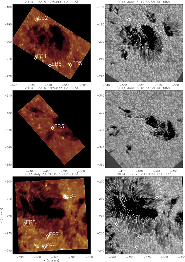
Figure 1. Regions observed in the Hα − 1.3 Å and TiO broadband filter. The white diamonds mark the locations where the EBs appeared.
Download figure:
Standard image High-resolution imageTo avoid any obscurity, we selected only these EBs that were sufficiently bright in Hα − 1.3 Å raster images and had contrast profiles of the well defined moustache shape. Figure 2 shows the profiles of nine selected EBs. The thin solid lines represent the background profiles used for the construction of the EB contrast profiles. The background profiles are obtained by taking an average of all profiles from a quiet Sun region within the FOV. Even though the contrast profiles of all the EBs are consistent with the known characteristics of a moustache, their details differ from one EB to another, particularly the maximum contrast and the asymmetry. The parameters of some selected properties are summarized in Table 1: date and time, position, the transverse speed of the associated EGFs (vtr), and the maximum contrast of the EBs in Hα and Ca ii profiles (CHα and CCa ii, respectively).
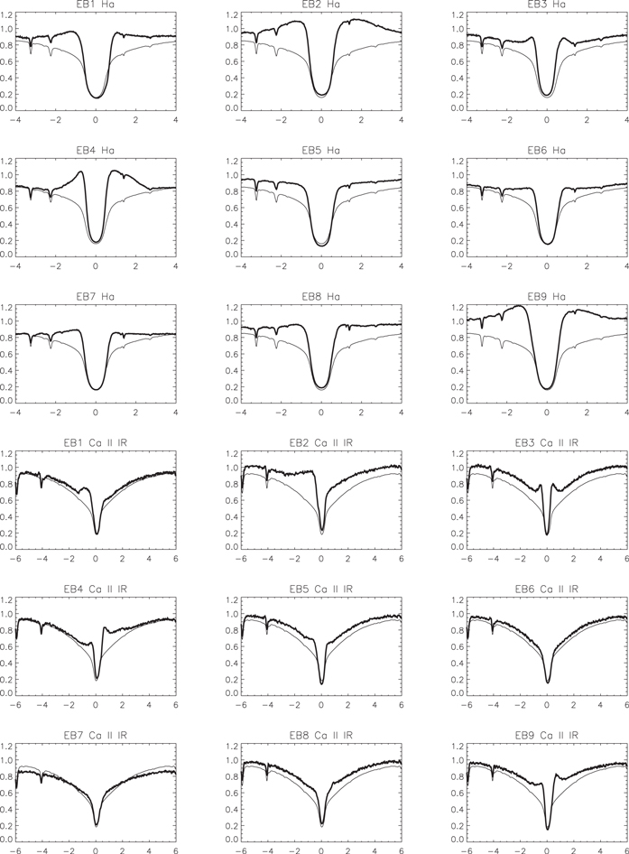
Figure 2. Profiles of the nine EBs under study (thick solid lines). The profiles are plotted for the locations where the ratio of Hα − 1.3 Å intensity to Hα − 4.0 Å intensity is maximal. Thin solid lines represent the background profiles.
Download figure:
Standard image High-resolution imageTable 1. Characteristics of Each Event
| Date | Event | Start Time | Position | vtr | CHα | CCa ii |
|---|---|---|---|---|---|---|
| EB1 | 2014 June 5 | 16:47:32 | (−527.5, −209.5) | 3.4 | 0.47 | 0.53 |
| EB2 | 2014 June 5 | 17:49:30 | (−526.9, −187.3) | 2.9 | 0.76 | 0.95 |
| EB3 | 2014 June 6 | 18:54:02 | (−396.5, −329.5) | 3.2 | 0.86 | 0.91 |
| EB4 | 2014 July 31 | 21:31:09 | (−364.1, −209.3) | 0 | 1.04 | 0.83 |
| EB5 | 2014 June 5 | 17:24:26 | (−207.1, −213.4) | 2.2 | 0.37 | 0.43 |
| EB6 | 2014 June 5 | 18:01:33 | (−519.1, −212.7) | 5.5 | 0.54 | 0.19 |
| EB7 | 2014 July 31 | 21:00:07 | (−375.2, −231.8) | 3.5 | 0.26 | 0.45 |
| EB8 | 2014 July 31 | 20:31:59 | (−387.5, −224.5) | 4.6 | 0.53 | 0.43 |
| EB9 | 2014 July 31 | 20:49:56 | (−376.0, −237.8) | ⋯ | 0.77 | 0.68 |
Download table as: ASCIITypeset image
The two left columns in Figures 3 and 4 show FISS raster images taken at Hα − 1.3 Å and the TiO band image. The size of EBs seen in Hα− 1.3 Å raster images ranges from 1'' to 3'', and all the EBs except EB6 display associated bright jet-like structures. EB1, EB3, EB4, and EB7 recurred several times during our observations, and EB2, EB3, EB4, and EB9 were accompanied by surges.

Figure 3. Hα − 1.3 Å raster and TiO broadband filter images of four EBs shown during the intensity peak (two left columns), and the d–t plots derived from TiO, Hα − 1.3 Å, NIRIS longitudinal magnetic field, and LOS velocity data (four right columns). The d–t plots are made along the white arrows shown in the raster images. The black and white solid lines in the d–t plots indicate the transverse motions of the EGFs approaching the site of the EBs.
Download figure:
Standard image High-resolution image3.1. EGFs
We found that each of the EBs was associated with a photospheric EGF. The moving front of an EGF usually approached the site of the EB just before its onset. We measured the transverse speed of each EGF following the intensity maximum in the distance–time (d–t) plots from the TiO filter shown in Figures 3 and 4. We excluded EB9 from the speed measurement because several moving features appeared near the site of EB9 and made it difficult to determine accurately which of the features was associated with the EB. The average speed of the transverse motions is found to be about 3.8 km s−1. Interestingly, most of the EGFs moved along the intergranular lanes.
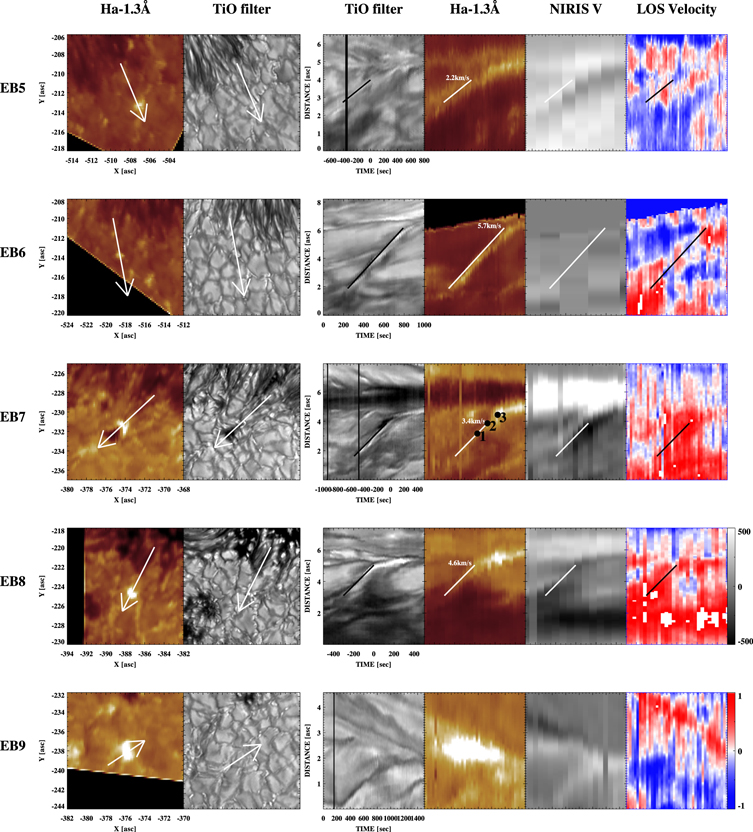
Figure 4. Raster images of the five EBs shown during the intensity peak at Hα − 1.3 Å rasters (two left columns), and the d–t plots derived from TiO, Hα − 1.3 Å, NIRIS longitudinal magnetic field, and LOS velocity data (four right columns).
Download figure:
Standard image High-resolution imageThe associated EGFs usually showed a brightening at the tip of their moving front as shown in the d–t plots from the TiO filter in Figures 3 and 4. The size of the brightening is less than 05. The brightening is also observed in the Hα and Ca ii 8542 Å spectral lines as an intensity enhancement. We also find that the brightening in TiO images is preceded by a weak darkening.
We classified eight events (excluding EB9) into two groups. Group 1 included EB1, EB2, EB3, and EB4, which were accompanied by EGFs with bi-directional expanding motions, and Group 2 contained EB5, EB6, EB7, and EB8 accompanied by EGFs with uni-directional motions observed in the TiO band image.
In Group 1, the bi-directional expanding motion of each EGF was identified from the chevron shape (<) in the d–t plots from the TiO filter (two black solid lines in Figure 3). The motion is a manifestation of the emergence of a bipolar magnetic element with its footpoints moving apart, since a pair of positive and negative magnetic elements appeared in the NIRIS V d–t plots along with every EGF. We also observed a photospheric upflow at the midpoint of the EGF, and photospheric downflows at its tips (see d–t plots from LOS velocity). The associated EB took place when the motion of the EGF decelerated sharply. In the case of EB2, a new granular cell emerged. But the deceleration of EB1 and EB3 was not linked to any changes in the granular structure (see Figure 5 and Section 3.2). EB4 showed the presence of a dark penumbral-like structure at the site of the EB. The maximum distance between the two tips of each EGF ranged from 3 to 5 arcsec (2–3.6 Mm).
Figure 5. Time sequence of EB3. The static figure compares the Ca ii − 0.05 Å (first row), Hα − 1.3 Å (second row), TiO broadband filter intensity (third row), photospheric LOS velocity measured at the Ti ii 6559 Å line (fourth row), and longitudinal magnetic flux (fifth row) of EB3. The animated online figure compares the TiO broadband, Hα, and longitudinal magnetic flux. The rasters of the longitudinal magnetic field at t = −325, −10, and 90 s were produced from HMI/SDO data.
(An animation of this figure is available.)
Download figure:
Video Standard image High-resolution imageIn contrast, the EGFs in Group 2 (EB5, EB6, EB7, and EB8) split off from the edge of the penumbra. The EGF in this case can be identified as a diagonal line in the d–t plot from the TiO filter in Figure 4. It moved together with a pair of positive and negative magnetic elements traveling in the sunspot's radial direction. In the case of EB5, EB7, and EB8, the pair of magnetic elements collided with the pre-existing strong magnetic field. The magnetic element that has the same polarity as the pre-existing magnetic field was followed by the element with opposite polarity. Then the magnetic element with the same polarity appears to infiltrate the pre-existing magnetic field. The associated EB took place abruptly when the EGF decelerated. We suspect that the EB might occur due to the magnetic cancellation between this opposite-polarity element and the pre-existing field line. On the other hand, EB6 brightened gradually, and then its Hα profile turned into moustache shape during its constant transverse motion. Thereafter the profile gradually returned to the normal shape. The d–t plots from the LOS velocity of EB7 and EB8 showed the strong downflows associated with the EGF, whereas those of EB5 showed weak downflow just behind the bright features of TiO filter images.
In the following sections, we describe two EBs in detail, one belonging to Group 1 and the other to Group 2.
3.2. EB3 in Group 1
EB3 was associated with a bi-directional expanding EGF, and hence belongs to Group 1. EB3 was observed on 2014 June 6 in the EF region near a pore.
Figure 5 shows the time sequence of the intensity maps, Dopplergrams, and magnetograms. Prior to the EB brightening, a bright loop-like structure was identified in the Ca ii raster images (black dotted curve at t = −19 s). One foot of the loop was rooted at the EB site, while the loop extended for about three arcseconds in the southwest direction. At t = 44 s, one can identify the EB onset with a bright jet structure ejected in the southeast direction and marked with black dotted line in Ca ii–0.05 Å raster images. The height of the jet is about 2''.
The time sequence of TiO images in Figure 5 shows the bi-directional expanding motion of the EGF of EB3. This EGF first appeared as a dark elongated structure between the regular granular cells (t = −341 s), then the two tips of the EGF moved apart from each other and developed a dumbbell shape (t = −13 s and t = 47 s). Because it is narrow, the EGF now looks like an intergranular lane rather than a granular cell (t = 47, 107 s). The two black arrows are pointing to the two moving fronts of the EGF. The bright tips and the thin dark lanes appeared at the moving fronts in the TiO filter images at t = −13 s. The distance between the tips of the bright feature and the dark lane is about 02, which is marginally resolvable with the 1.6 m telescope. The bi-directional expanding motion of the EGF in this area looks similar to the report of Yurchyshyn et al. (2012).
The observed behavior of the EGF is quite similar to what we expect to see when a bipolar flux emerges through the photosphere. One can easily identify photospheric upflows in the middle of the black slit that corresponds to the center of the EGF in the raster at t = −19 s. Moreover, the NIRIS maps of longitudinal magnetic field at t = −224 and 90 s show that a negative magnetic element appeared at the tip of the EGF. This element is not resolved in HMI because of its limited spatial resolution. We also find a diffuse and very weak positive magnetic element at the other tip of the EGF in the d–t plot for EB3 (Figure 3).
3.3. EB7 in Group 2
EB7 was included in Group 2 and it was associated with a uni-directional expanding EGF. The EB was first observed at 21:00:07 UT on 2014 July 31 at a certain distance from the penumbra.
Figure 6 shows the raster images of EB7. In TiO images, a small pore was located at (−375'', −232'') near the outer edge of the penumbra, and EB7 was detected on the northwest side of this pore (Hα − 1.3 Å image at t = 91 s). As indicated by the black arrows in the TiO images, an EGF first appeared as a part of the penumbral filament at t = 316 s before the EB occurred, then the tip of the EGF moved toward and collided with the pore at the time the EB occurred. The tip of the EGF included a bright core surrounded by a thin dark lane similarly to EB3. The core is also clearly distinguishable in the TiO d–t plot. The transverse speed of the EGF is about 3.4 km s−1.
Figure 6. Time sequence of EB7. The static figure compares the Ca ii − 0.05 Å (first row), Hα − 1.3 Å (second row), TiO broadband filter intensity (third row), photospheric LOS velocity measured at the Ti ii 6559 Å line (fourth row), and longitudinal magnetic flux (fifth row) of EB7. The animated online figure compares the TiO broadband, Hα, and longitudinal magnetic flux.
(An animation of this figure is available.)
Download figure:
Video Standard image High-resolution imageA pair of a negative and positive magnetic elements emerged at about t = −800 s and moved co-spatially with the corresponding EGF (see red dotted circles in the NIRIS V images). The transverse motion of this pair is also prominent in the d–t plot of longitudinal magnetic flux in Figure 4. When the pair approached the pore, the positive element appeared to infiltrate the pore of the same positive polarity, while the negative element following behind the positive one might remain around, and then it might cancel out with the positive pore flux. Such magnetic behavior is similar to the emergence of a concave part of an undulating magnetic field—in other words, a U-shaped loop. This magnetic configuration is often adopted to explain bipolar MMFs (Shine & Title 2001; Lim et al. 2011). We found persistent downflows of about 1 km s−1 associated with the EGF. The downflows may be explained as the plasma draining along the field lines.
3.4. Time Variations of the Hα and Ca ii Profiles
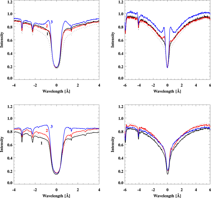
Figure 7 shows time variations of the Hα and Ca ii line profiles at the tip of the EGFs. In the case of EB3, the initial Hα spectrum marked as 1 (black solid line) appeared as a normal Hα absorption line profile, but the intensity at every wavelength except for the line core was higher than that of the comparison profile. The second profile (red solid line) was enhanced as well. The third plotted profile (blue solid line) taken just after the EB maximum was of higher intensity than the first two in the far wings and of much higher intensity in the near wings. The core intensity, however, changed little; this is known as the moustache shape. The Ca ii spectrum shows a similar pattern.
Figure 7. Hα (left) and Ca ii (right) line profiles taken at the positions and times marked 1–3 in the Hα − 1.3 Å d–t plot of EB3 in Figure 3 (two upper plots) and EB7 in Figure 4 (two lower plots). The black dashed lines are the normalized averaged profiles plotted for comparison. The first profile (black solid line) was measured at the initial phase of the EGF. The second profile (red solid line) was measured just before the EB onset. The third profile (blue solid line) was taken at the peak of the EB.
Download figure:
Standard image High-resolution image
The enhancement of the far wings (>±2.5 Å) of the second line profile is characterized by the brightness temperature excesses of about 72 K and 121 K in the Hα and Ca ii over the comparison profile, while the TiO intensity is characterized by a temperature excess of 288 K. The far wings of the third profile are also characterized by temperature increases of about 144 K and 294 K, respectively.
In the case of EB7, we observe higher intensity in the far wings of the second Hα profile (just before the EB occurrence) and the third one (just after the EB) than in the first profile, which is similar to EB3. The intensity of the line core also remained the same. Note that the first spectrum appeared dark in the far wings of both lines as compared to the comparison profile (black dashed lines), because the lines darkened due to the penumbra-like features in the photosphere.
In this case, the increase in intensity of the far blue wings (>±2.5 Å) of the second spectrum in both lines is characterized by the temperature excesses of about 99 K and 165 K over the first spectrum, respectively. The increase in TiO filter intensity corresponds to 288 K for the second point and 252 K for the third point.
4. SUMMARY AND DISCUSSION
We report on the photospheric transverse motions of the EGFs associated with the EBs. The average speed of the motions is about 3.8 km s−1. Even though our study does not sample a large number of EBs, it suggests that a majority of them are probably accompanied by EGFs. The average speed of the EGFs is consistent with previous studies (Guglielmino et al. 2010; Yang et al. 2013; Kim et al. 2015). It is interesting that the EGFs show much faster motions than a typical granular motion of about 1 km s−1.
The observed events were classified into two groups. The events of Group 1 were accompanied by bi-directionally expanding EGFs, while the events of Group 2 were accompanied by uni-directionally expanding EGFs. In Group 1, EGFs appear to result from the emergence of flux, which is evident from the bi-directional motion, the upflows at the middle point of an EGF, downflows at the tips, and the bipolar magnetic elements. The EBs that developed abruptly at the tip of the EGF reached and stopped at the site. The EBs are likely to be caused by magnetic reconnection between the EF and the pre-existing fields, as suggested by Yokoyama & Shibata (1995). Meanwhile, the events in Group 2 seem to be associated with bipolar MMFs characterized by a pair of magnetic elements and uni-directionally expanding EGFs. The MMFs are likely to be a part of a serpentine field, which is an extended penumbral field carrying the Evershed flow (Lim et al. 2011). The MMFs may move radially as a result of the rising of the penumbra into the upper atmosphere. Then EBs took place when the tip of the EGFs approached and stopped at their location.
Our results of Group 1 support the idea that magnetic reconnection manifested by EBs occurs at the bald patch when the flux tube emerges into the low atmosphere (Pariat et al. 2004; Isobe et al. 2007). The EF might be subjected to the magnetic buoyancy instability considering the scale of the observed EF of about 3–5 arcsec, which is longer than the scale of the Parker unstable wavelength of about 2 Mm (Pariat et al. 2004). In addition, the blueshift in the middle and the redshift at the foot of the flux tube also show good agreement with the simulation result of Isobe et al. (2007). The fast transverse motions of the EGFs reported here indicate that the flux tube may emerge abruptly.
One of the important results is that the EBs are associated with bipolar MMFs. In our observational data for Group 2, three out of four MMFs approached small pores that had the same polarity as the main sunspot. Previous studies showed that the pore-satellites and MMFs usually have this type of polarity configuration (Harvey & Harvey 1973). This result indicates that magnetic reconnection takes place between the trailing magnetic element of MMFs and the pre-existing field lines, at the location of the U-shaped loops. We note that Nindos & Zirin (1998) reported the association between EBs and unipolar MMFs. Most of the MMFs are likely to have bipolar polarity as in our results (Harvey & Harvey 1973; Yurchyshyn et al. 2001). Our findings also differ from those of Bernasconi et al. (2002), who found that dipolar MMFs flowed into a sunspot, then EBs took place at the foot of an Ω-shaped loop.
The fast transverse motion of EGFs is interesting because their speed is comparable to the sound speed of the photosphere (cs ∼ 8.5 km s−1; Cox 2000). The transverse motion of the magnetic elements will leave a trace as EGFs in the photosphere. In that regard, the local magnetic pressure dominates the plasma pressure at the base of the flux tubes even though plasma β is much higher than unity in the photosphere (Gary 2001). We conjecture that this motion of the magnetic elements, or abrupt emergence of the flux tubes, forces the magnetic reconnections that are identified as EBs.
We report brightenings at the tip of the EGFs seen in TiO filtergrams as well as in the far wing of the Hα and Ca ii lines prior to the EBs. These brightenings have been reported in previous studies (Lim et al. 2011, 2012; Yang et al. 2013). Lim et al. (2011) detected a slight brightening in the TiO and Hα filtergrams. Yang et al. (2013) characterized the temperature excess ΔT ∼ 200 K in the far wings of the Ca ii line when an EB developed. Here we measured an increase in temperature of a few hundred kelvin in TiO filter images. The far wings of the Hα and Ca ii lines also showed uniform enhancement, which differs from the near-wing (<±2.5 Å) enhancements of moustache shapes of EBs. These brightenings and the far-wing enhancements might be small-scale magnetic concentrations (MCs) with lower density associated with continuum enhancements due to the radiative hot wall heating in the absence of convective heating (Spruit 1974). MCs are also manifested as strikingly intense small-scale brightenings in the blue wing of the Hα line at the location of the intergranular lanes (Leenaarts et al. 2005).
Our study also suggests that one has to be cautious in distinguishing between EBs and MCs. Recent studies using filtergrams have introduced an ambiguity in defining the EBs because the brightenings seen at a specific wavelength such as Hα − 0.7 Å or Hα − 1.4 Å appear similar to MCs (Nelson et al. 2013; Rutten et al. 2013). We find that a line profile may have a constant enhancement at every wavelength even prior to the occurrence of EBs. This enhancement does not indicate an EB, but rather an intensity enhancement in an MC. We suggest that observations in at least three spectral ranges are necessary to confirm the presence of an EB: the far wings (>±2.5 Å), the near wings (<±2.5 Å), and the core (0 Å) of a spectral line.
One interesting result of our study is that bi-directional and uni-directional photospheric motions of EGFs seem to emerge in the intergranular lanes. It seems that the EFs or MMFs prefer to travel in the intergranular lanes (Otsuji et al. 2007; Kim et al. 2015; Reid et al. 2015). Moreover, Watanabe et al. (2011) reported that an EB moved along the intergranular lanes. We suspect that the granular convection motions may guide the motion of the flux tubes along the granular lanes.
In conclusion, we have shown the fine-scale connections among the photospheric features—EFs, MMFs, and EBs. Our result suggests a picture where an EB is a response of the atmosphere to the process of magnetic reconnection forced by the EFs or MMFs manifested by the EGFs.
This work was supported by the National Research Foundation of Korea (NRF-2012 R1A2A1A 03670387).
Facilities: Big Bear Solar Observatory -