


ABSTRACT
We present the results of the Swift and NuSTAR observations of the nearby BL Lac object Mrk 421 during 2013 January–June. The source exhibited a strong long-term variability in the 0.3–10 keV and 3–79 keV bands with the maximum-to-minimum daily-binned flux ratios of 22 and 95, respectively, in about 3 months, mainly due to unprecedented strong X-ray outbursts by more than an order of magnitude in both bands within 2 weeks in 2013 April when the 0.3–10 keV count rate exceeded the level of 200 cts s−1 for the first time, and Mrk 421 became one of the brightest sources in the X-ray sky. The source was also very active on intra-day timescales, and it showed flux doubling and halving timescales of 1.16–7.20 hr and 1.04–3.54 hr, respectively. On some occasions, the flux varied by 4%–23% within 300–840 s. During this period, the source also exhibited some of the most extreme X-ray spectral variability ever reported for BL Lacs—the location of the synchrotron spectral energy distribution peak shifted from a few eV to ∼10 keV, and the photon index at 1 keV and curvature parameter varied on timescales from a few weeks down to intervals shorter than 1 ks. MAGIC and First G-APD Cherenkov Telescope observations also revealed a very strong very high energy (VHE) flare during April 11–17. The UV and HE γ-ray flares were much weaker compared to their X-ray counterparts, and they generally showed significantly stronger correlation with each other than with the X-ray fluxes.
Export citation and abstract BibTeX RIS
1. INTRODUCTION
BL Lacertae objects (BL Lacs, BLLs) constitute a rare class of active galactic nuclei (AGNs) with observational features like weak or absent emission lines, high radio and optical polarization, superluminal motions, and a typical double-humped spectral energy distribution (SED) dominated by a non-thermal radiation from the radio to γ-ray frequencies that makes them the most frequently detected class of the extragalactic TeV sources (Falomo et al. 2014). These features are generally attributed to non-thermal radiation from a relativistic jet nearly pointed along the line of sight (Urry & Padovani 1995, and references therein). The lower-frequency component of BLL SEDs is explained via synchrotron radiation emitted by relativistic electrons in the jet (Celotti & Ghisellini 2008), while there are a variety of models for the origin of the higher-energy bump: an inverse Compton (IC) scattering of synchrotron photons by the same electron population (so-called synchrotron self-Compton model, SSC; Marscher & Gear 1985); ambient photons scattered by the jet ultra-relativistic electrons (external Compton, EC; Dermer et al. 1992); synchrotron radiation from highly relativistic protons (Aharonian 2000), etc. Hadronic processes have also been considered, including photomeson production, neutral pion decay, and synchrotron-pair cascading (e.g., Mannheim & Biermann 1992). We can draw conclusions about the validity of these models via the study of flux variability characteristics in different spectral bands and their cross-correlations, which also can provide important clues about the physics, the structure, and the dynamics of the BLL emission zone.
In this paper, we present the results related to the X-ray timing and spectral behavior of the nearby high-energy peaked BLL (HBL) source (i.e., a BLL with a synchrotron component peaking in at the UV–X-ray frequencies; Padovani & Giommi 1995) Mrk 421 (z = 0.031, Aleksic et al. 2015a) in the first half of 2013 when it was observed intensively with the X-ray Telescope (XRT; Burrows et al. 2005) onboard the Swift satellite (Gehrels et al. 2004) and the NuSTAR observatory (Harrison et al. 2013). In this period, the source was very active in X-rays, and the different aspects of its multiwavelength (MWL) behavior were presented by Pian et al. (2014), Paliya et al. (2015), Sinha et al. (2015), Balocovic et al. (2016) (herafter B16), and Hovatta et al. (2015). Along with the 0.3–10 keV and 3–79 keV data obtained with the aforementioned instruments, we have processed and analyzed those obtained with the Ultraviolet-Optical Telescope (UVOT; Roming et al. 2005) and Large Area Telescope (LAT) onboard Fermi (Atwood et al. 2009). We have also used the publicly available light curves from the observations performed with the Burst Alert Telescope (BAT; Barthelmy et al. 2005) onboard Swift, Monitor of All Sky X-ray Image (MAXI; Matsuoka et al. 2009), MAGIC (Lorenz 2004), First G-APD Cherenkov Telescope (FACT; Anderhub et al. 2013), and the OVRO 40 m telescope (Richards et al. 2011) during the 2013 January–June period to draw conclusions about the interband correlations.
The paper is organized as follows. Section 2 describes the data processing and analyzing procedures. In Section 3, we provide the results of a timing analysis and those from the X-ray spectroscopy in Section 4. We discuss our results in Section 5, and provide our conclusions in Section 6.
2. OBSERVATIONS AND DATA REDUCTION
2.1. X-Ray Data
We retrieved the Swift-XRT data from the publicly available archive, maintained by HEASARC.5 The Level 1 unscreened event files were processed with the XRTDAS package v.2.5.1 developed at the ASI Science Data Center (ASDC) and distributed by HEASARC within the HEASOFT package (v.6.17). They were reduced, calibrated, and cleaned by means of the XRTPIPELINE script using the standard filtering criteria and the latest calibration files of Swift CALDB v.20150721. We selected the events with the 0–2 grades for the Windowed Timing mode, used to observe Mrk 421 in this period.
The source and background light curves and spectra were extracted with XSELECT using circular areas with radii of 30–70 pixels depending on the source brightness and exposure. For the fluxes ≳100 cts s−1, the source events were extracted from an annular region with inner radius ranging from 1 to 3 pixels according to the prescription of Romano et al. (2006). The light curves were then corrected using the XRTLCCORR task for the resultant loss of effective area, bad/hot pixels, pile-up, and vignetting. The ancillary response files (ARFs) were generated using the XRTMKARF task, with corrections applied to account for the point-spread function (PSF) losses, different extraction regions, vignetting, and CCD defects. The instrumental channels were combined to include at least 20 photons per bin using the GRPPHA task. After selecting the best-fit model for the fixed hydrogen absorption column density  and deriving the values of corresponding spectral parameters (see Section 4 for details), we calculated the unabsorbed 0.3–2 keV, 2–20 keV, and 0.3–10 keV fluxes and their errors by means of the cflux model.
The NuSTAR data were processed with the NuSTARDAS package v.1.5.1 available within HEASOFT. We used CALDB (v.20151008). After running nupipeline, the nuproducts task was used to obtain light curves and spectra in the energy range 3–79 keV. The source events were extracted from circular regions with radii of 40–80 arcsec, depending on the source brightness and exposure. The background counts were extracted from a concentric area, centered on the source, with inner and outer radii of 90 and 120 arcsec, respectively. The ARFs were generated with the numkarf task, applying corrections for PSF losses, exposure maps, and vignetting. Similar to Brenneman et al. (2014), we have not combined responses or spectra from FPMA and FPMB, but instead fitted them simultaneously in order to minimize systematic effects taking into account a cross-calibration factor of 1.07 for FPMB relative to FPMA, derived by these authors. The spectral analysis and the extraction of unabsorbed 3–10 keV, 10–79 keV, and 3–79 keV flux values was done similar to the XRT observations.
The BAT data, taken from the Swift-BAT Hard X-ray Transient Monitor program6 (Krim et al. 2013), have been re-binned using the tool REBINGAUSSLC from the HEASOFT package using the weekly bins.
From the publicly available daily-binned 2–20 keV light curves of Mrk 421 obtained with MAXI7 , we used only those corresponding to the source's detection above 5σ significance for a flux variability study.8
2.2. Swift-UVOT Data
The photometry for the sky-corrected images obtained in the UVOT bands UVW1, UVM2, and UVW2 was performed via the UVOT software developed and distributed within HEASOFT and the calibration files included in the CALDB. The UVOTSOURCE tool was used to extract the source and background counts, correct for coincidence losses, apply background subtraction, and calculate the corresponding magnitude. The measurements were performed via a 20 arcsec radius. The magnitudes were then corrected for Galactic absorption, applying  mag, and the
  values, calculated using the interstellar extinction curves provided in Fitzpartick & Messa (2007), and the effective wavelength of each UVOT filter, were taken from Poole et al. (2008). We converted them into linear fluxes (in mJy) adopting the latest photometric zero-points for each band provided in Breeveld et al. (2011). From the obtained values, we subtracted 0.09, 0.05, and 0.06 mJy for the UVW1, UVM2, and UVW2 bands, respectively, derived from UVW1 = 17.44 mag, UVM2 = 17.98 mag, and UVW2 = 17.72 mag to remove the host contribution (Cesarini 2013).
2.3.
 -ray Data

We extracted 0.3–300 GeV fluxes from the LAT observations using the events of the diffuse class from a region of interest (ROI) of radius 10°, centered on the coordinates of Mrk 421, and processed with the Fermi Science Tools package (version v10r0p5) with P8R2_V6 instrument response function using an unbinned maximum likelihood method. A cut on the zenith angle (>100°) was applied to reduce contamination from the Earth-albedo γ-rays. The data taken when the rocking angle of the spacecraft is larger than 52° are discarded to avoid contamination from photons from the Earth's limb. A background model including all γ-ray sources from the Fermi-LAT 4 years Point Source Catalog (3FGL, Acero et al. 2015) within 20° of Mrk 421 was created. The remaining excesses in the ROI were modeled as point sources with a simple power-law (PL) spectrum. The spectral parameters of sources within the ROI were left free during the minimization process while those outside of this range were held fixed to the 3FGL catalog values. A log-parabolic (LP) function was used for nearby sources with significant spectral curvature and a PL for those sources without it. The Galactic and extragalactic diffuse γ-ray emission as well as the residual instrumental background are included using the recommended model files gll_iem_v06.fits and iso_P8R2_SOURCE_V6_v06.txt. The normalizations of both components in the background model were allowed to vary freely during the spectral fitting. The detection significance of the target σ was calculated as  where TS is the test-statistics (Abdo et al. 2009). For the spectral modeling of Mrk 421, we adopted a simple PL, as done in the 3FGL catalog.
During 2013 January–June, the source was observed at TeV energies for 200 hr with the FACT (Anderhub et al. 2013), located in the Observatorio del Roque de los Muchachos (La Palma, Spain). The FACT collaboration publishes the results of a preliminary quick-look analysis with small latency on a website.9 These background-subtracted light curves are not corrected for the effect of changing energy threshold with changing zenith distance and ambient light, and no data selection is done. Details on the analysis are described in Dorner et al. (2015).
For our study, we have used only signals detected with a minimum significance of 3 standard deviations. From the daily-binned data, we used 28 nights. More than 97% of these data are taken with a zenith distance small enough to not influence the energy threshold of the analysis. More than 82% of the data are taken under light conditions not exceeding the analysis threshold. For the rest of the data, the analysis threshold increases with increasing zenith distance and increasing amount of ambient light. Therefore, seven of the data points might be up to a factor 2 higher when the fluxes are calculated taking into account the energy threshold. From the data binned in 20 minutes, we used the data of two nights corresponding to 8 hr. All of these data are taken under light conditions with a stable energy threshold and more than 95% have a zenith distance not changing the energy threshold.
3. MWL TEMPORAL STUDY
The source was observed 68 times by XRT between 2013 January 2 and May 16 with a total exposure of 199 ks. The information about each pointing and the corresponding count rates are provided in Table 1. The same table also contains the results of the UVOT observations including the de-reddened magnitudes and corresponding fluxes for each band. Mrk 421 was the NuSTAR target 23 times between January 2 and April 19, amounting to 383.4 ks of exposure. Table 2 presents the information about each observation with corresponding measurement results.
Table 1. Extract from the Summary of the XRT and UVOT Observations
| ObsID | Obs. Start–End | Exp. | CR |

|

|

|

|

|

|
|---|---|---|---|---|---|---|---|---|---|
| (UTC) | (s) | (cts s−1) | (mag) | (mJy) | (mag) | (mJy) | (mag) | (mJy) | |
| (1) | (2) | (3) | (4) | (5) | (6) | (7) | (8) | (9) | (10) |
| 80050001 | 01-02 18:52:59 01-02 21:25:38 | 1814 | 10.46(0.09) | 10.93(0.04) | 37.93(0.94) | 10.87(0.04) | 34.31(0.64) | 10.88(0.04) | 32.75(1.01) |
| 35014024 | 01-04 22:25:59 01-05 00:03:34 | 1064 | 19.71(0.15) | 10.85(0.04) | 40.84(1.60) | 10.96(0.04) | 31.57(0.64) | 10.91(0.04) | 31.86(1.06) |
Note. The columns are as follows: (1)—Observation ID (the three leading zeroes are omitted); (2) and (3)—Observation beginning and end, respectively (in UTC); (3)—Exposure time (in seconds); (4) Observation-binned count rate with its error; (5)–(10)—de-reddened UVOT magnitudes and corresponding fluxes (in mJy).
Only a portion of this table is shown here to demonstrate its form and content. A machine-readable version of the full table is available.
Download table as: DataTypeset image
Table 2. Extract from the Summary of the NuSTAR Observations
| ObsID | Obs. Start–End | Exp. | CR |
|---|---|---|---|
| (UTC) | (s) | (cts s−1) | |
| 60002023002 | 01-02 18:41:07 01-02 23:01:07 | 9152 | 0.42(0.01) |
| 60002023004 | 01-10 01:16:07 01-10 13:41:07 | 22633 | 0.40(0.01) |
Only a portion of this table is shown here to demonstrate its form and content. A machine-readable version of the full table is available.
Download table as: DataTypeset image
Figure 1(a) presents the daily-binned light curve from the XRT observations. The 0.3–10 keV flux was highly variable, changing by a factor of about 22, and showed several flares which are discussed in detail below. During the six month period, the highest and weighted mean fluxes were 165.44 cts s−1 (April 13) and 23.66 cts s−1, respectively. In the case of 60 minutes binning, the highest flux of 260.71 ± 2.79 cts s−1 was recorded during the eighth orbit of ObsID 00080050019 (MJD 56395.3), and this observation corresponds to the first occasion when the 0.3–10 keV flux exceeded the level of 200 cts s−1. A significantly larger variability was observed by NuSTAR (Figure 1(b))—the 120 minutes binned 3–79 keV count rate changed by a factor of 194.6 between 0.30 ± 0.02 cts s−1 (the fifth orbit from ObsID 60002023008 (MJD 56312.1)) and 58.38 ± 0.16 cts s−1 (the ninth orbit from ObsID 60002023031(MJD 56396.9)). The daily-binned 3–79 keV flux varied by a factor of 95. Therefore, Mrk 421 is the brightest and the most violently variable blazar in X-rays. MAXI detected it with 5σ significance only during March 27–April 21 (when the source was the most variable in X-rays) and June 4–25 (not being accompanied with XRT and NuSTAR observations) periods (Figure 1(c)). The maximum-to-minimum flux ratio R = 4.27, and this modest value is clearly related to significantly lower instrumental characteristics of MAXI compared to XRT and NuSTAR. The detection of Mrk 421 with 5σ significance from daily-binned BAT data occurred only four times during the giant X-ray outbursts of April 11–17 with  3.
3.

Figure 1. The light curves from the 2013 January–June observations of Mrk 421 performed with Swift-XRT (upper panel), NuSTAR (panel (b)), MAXI (panel (c)), UVOT (UVW1 and UVW2 bands; panel (d)), OVRO (panel (e)), Fermi-LAT (0.3–300 GeV; panel (f)), MAGIC and VERITAS (panel (g); the data above the threshold E = 200 GeV from B16 are given with gray asterisks, while those from MAGIC observations above E = 300 GeV from Preziuso (2013)—with black points), and FACT (panel (h)). The vertical dashed lines indicate the periods discussed in Section 3.
Download figure:
Standard image High-resolution imageFigure 1(d) shows the light curves from the UVW1 and UVW2 bands.10 Although the largest UV fluxes are observed in the epoch of the aforementioned giant X-ray outbursts, the source varied on significantly longer timescales at these frequencies, and the lowest UV state was recorded in the epoch of one of the X-ray flares preceding the giant outbursts by about 3 months (see below). The UV flux ranges are much smaller compared to the X-ray ones—the ratio R is equal to 3.06 and 3.08 for the UVW1 and UVW2 bands, respectively. Even weaker variability is evident from Figure 1(e) which presents the 15 GHz light curve from the OVRO observations.11 The flux varied only by a factor of 1.32, the maximum flux was recorded 2 months later than the giant X-ray outbursts, and no flaring activity was seen in the radio band during the latter events.
Although the 3 days binned LAT light curve mainly shows the presence of γ-ray flares in the epochs of X-ray ones, and the highest 0.3–300 GeV brightness state nearly coincides with that of XRT and NuSTAR bands, the flare amplitudes are much smaller with  = 3.90, and the flare peak in the April 11–18 epoch shows almost the same height as the one observed along with the preceding X-ray flare (Figure 1(e)). On average, Mrk 421 showed one of the highest test-statistics since the start of the LAT observations in 2013 January–March, and it was detectable with 3σ significance from one-day binned data in the periods discussed in Section 3.1. The very high energy (VHE) light curve shows two flares exhibiting flux changes by a factor of 8.7 and 4.3, respectively (Figure 1(g)), although the amplitude of the second event might be larger, since the corresponding light curve consists of only a few data points and the flare was observed incompletely. This is evident from Figure 1(h) which shows a very strong outburst and subsequent fast decay to the initial level by a factor of 18.2 in the daily-binned VHE excess rate from the FACT observations which show a peak at MJD 56397 (separated by about 2 days from the peak of the previous light curve).12
Below, we concentrate on the results from the different periods (based on the occurrence of longer-term flares in the XRT band) from the 2013 January–May period whose summary is presented in Table 3. For each flare, the fractional root mean square (rms) variability amplitude and its error were calculated the same way as in Vaughan et al. (2003) and reported in Table 3
with S2—the sample variance;  —the mean square error;
  —the mean flux. The MWL light curves from each period are provided in Figure 2.

Download figure:
Standard image High-resolution image
Figure 2. MWL variability of Mrk 421 in different epochs. In each UVOT panel, the UVW1-band light curve is plotted with black points, and a gray color is used for the UVW2 band.
Download figure:
Standard image High-resolution imageTable 3. Summary of the XRT and UVOT Observations in Different Periods (Column 1)
| XRT | UVOT | NuST. | LAT | |||||||||
|---|---|---|---|---|---|---|---|---|---|---|---|---|
| Per. | Dates | Nfl | Fmax | R | Fvar |

|

|

|

|

|

|

|
| (1) | (2) | (3) | (4) | (5) | (6) | (7) | (8) | (9) | (10) | (11) | (12) | (13) |
| 1 | Jan 2–18 | 2 | 26.38 | 3.68 | 50.3(0.5), 38.4(0.3) | 2.85 | 5.40 | 1.65 | 1.53 | 2.93 | 1.69 | 5.23 |
| 2 | Jan 22–Feb 14 | 1 | 35.09 | 3.33 | 35.6(0.4) | 4.06 | 4.58 | 1.76 | 1.76 | 3.43 | 1.73 | 9.17 |
| 3 | Feb 27–Mar 15 | 1 | 34.46 | 3.10 | 31.1(0.3) | 3.00 | 3.18 | 1.39 | 1.38 | 1.51 | 1.32 | 7.5 |
| 4 | Mar 15–Apr 7 | 1 | 84.94 | 7.18 | 43.1(0.1) | 6.59 | 8.51 | 1.32 | 1.37 | 5.70 | 1.36 | 5.40 |
| 5 | Apr 10–19 | 3 | 260.72 | 13.45 | 45.1(0.2)–77.4(0.1) | 7.60 | 30.92 | 1.71 | 1.77 | 1.50 | 84.43 | 3.08 |
| 6 | Apr 21–May 11 | 2 | 34.51 | 3.34 | 29.8(0.5), 33.0(0.4) | 2.96 | 5.32 | 1.50 | 1.59 | 1.68 | ⋯ | 4.10 |
Note. Column 3: number of X-ray flares in the particular period; Columns 4–6: maximum 0.3–10 keV flux from the 1 minute-binned light curves (in cts s−1), maximum-to-minimum flux ratio, and fractional amplitude (%) for each flare, respectively; Columns 7–8: maximum-to-minimum flux ratios for unabsorbed 0.3–2 keV and 2–10 keV fluxes; Columns 9–11: the same for the UVOT bands, and those for NuSTAR and LAT in Columns 12 and 13, respectively.
Only a portion of this table is shown here to demonstrate its form and content. A machine-readable version of the full table is available.
Download table as: DataTypeset image
3.1. Longer-term X-Ray Activity
3.1.1. The Epoch Before the Giant X-Ray Outbursts
The source showed two consecutive 0.3–10 keV flares exhibiting flux variation by a factor of 2.9 and 3.5 centered on MJD 56297 and MJD 56307 in Period 1 (see Table 3 and Figure 2(a), upper panel). The highest optical–UV states were seen in the epoch of the first X-ray flare, which were followed by a long-term decay till the end of this period, and no increasing activity was observed in any UVOT band along with the second X-ray flare. The LAT-band light curve showed a flare in the epoch of the first 0.3–10 keV event, and the another one in the beginning of the second X-ray flare. Afterwards, we observe a low 0.3–300 GeV state along with the highest X-ray fluxes in this epoch. A similar situation is found in Period 2 (see Table 3) when the 0.3–10 keV flare exhibited a flux change by a factor of 3.4 (that was longer than those in the previous period; see Figure 2(b)), which coincided with the lowest UV and HE (on average) brightness states during the whole 2013 January–June period (see the corresponding discussion in Section 5.1). In contrast, the VHE γ-ray light curve followed the X-ray one (Figure 2(b), bottom panel). The source was active in all spectral bands in Period 3 (see Table 3) when the X-ray flare exhibiting a flux change by a factor of 3.1 was accompanied with those in the UVOT and LAT bands by a factor of ∼1.4 and 7.5, respectively (Figure 2(c)).
In Period 4 (see Table 3), the source showed a flare with flux variation by a factor of 6.6 in the XRT band, and the largest FACT excess rates are observed in the epoch of the X-ray peak (Figure 2(d)). The LAT-band flux also showed flares with flux variation by a factor of 3.6–5.3 in this period, and it reached the highest brightness state in 2013 January–June. One of the 0.3–300 GeV peaks almost coincided with the epoch of the highest X-ray, VHE, and UV fluxes in this period (on MJD 56383). However, we observe a minor UV and γ-ray peak in the beginning of this period, followed by a decay during the next days (along with the same trend in the FACT excess rates, provided in the upper panel of Figure 2(d)) while the X-ray flux showed an increasing trend.
3.1.2. Giant X-Ray Outbursts and the Subsequent Epoch
The source exhibited an unprecedented X-ray flaring behavior in Period 5 (see Table 3) when we observe two consecutive outbursts by with increasing flux a factor of 12 and 8.1 (with respect to the flux value recorded on April 7) centered on MJD 56395.5 ("Flare 1") and MJD 56397.3 ("Flare 2"), respectively (Figure 2(e), top panel). Afterwards, a relatively minor flare was seen around MJD 56399.4 ("Flare 3"). The 3–79 keV light curves followed closely those from the XRT observations. However, Flares 2 and 3 were significantly stronger compared to their 0.3–10 keV counterparts, and the second 3–79 keV flare was significantly stronger than the first one (in contrast to the XRT band) (Figure 2(e), middle panel), and the latter showed practically the same amplitude as the third flare. The MAXI light curve exhibits two peaks in the epochs of Flares 1 and 2 (Figure 2(e), bottom panel). The source also showed a strong VHE flare wth increasing flux at least by a factor13 of 4.3 along with Flare 1 (Figure 2(f), bottom panel). The maximum flux value was 2.64 times larger than that of the VHE flare seen in Period 3. In fact, this difference should be larger, since the corresponding light curve is constructed using the fluxes above the 300 GeV threshold (from Preziuso 2013) while the light curve from Period 3 consists of data above 200 GeV. The FACT observations show the peak in the TeV excess rate two days later (on the day of the Flare 2 peak) than that revealed by the MAGIC observations (coinciding with the X-ray peak of Flare 1). Note that this was the strongest TeV flare during the 4.5 years of FACT observations of Mrk 421 (see Figure 3). The maximum value of the 15–150 keV count rate from the daily-binned BAT observations coincided with the peak of Flare 2.14

Figure 3. Historical light curve of Mrk 421 constructed with daily-binned FACT excess rates corresponding to detections with at least 3σ significance. Its part between the vertical red dashed lines corresponds to Period 5.
Download figure:
Standard image High-resolution imageIn contrast to the X-ray and VHE data, the 0.3–300 GeV flux from this period was not the highest in the first half of 2013. Its maximum value from the daily-binned data (recorded in the epoch of a decay phase of Flare 1 and increasing part of Flare 2) was 16% lower compared to that from Period 3. The optical–UV light curves also show an uncorrelated behavior with the X-ray ones. They peaked in the beginning of the period and we then observe a decay, followed by a plateau-like bahaviour in the epoch of Flares 1–3. No significant variability was observed at 15 GHz, and the radio flux was close to its minimum value during the 2013 January–June period.
In the second half of this period (April 16–22), Mrk 421 was the target of the intensive INTEGRAL campaign whose detailed results are provided by Pian et al. (2014). During these days, the source showed a strong flare in the JEM-X and ISGRI bands (5.52–100 keV energy range), coinciding with Flare 3. The same authors also reported two subsequent V-band flux flares (from the INTEGRAL-OMC observations) whose peaks occurred about 0.5 and 3.5 days later than the X-ray one, respectively.
The source showed two consecutive flares in Period 6 (see Table 3) in X-rays with R = 3.44 (Figure 2(g)). The peaks of the UV and LAT light curves were observed in the epoch of the first flare, and there is another 0.3–300 GeV peak separated by about a day from that of the second X-ray flare. Similar to Periods 4 and 5, the source was also detected by MAXI with 5σ significance frequently in 2013 June, and it showed a flare with flux increase by a factor of 2.2 centered on MJD 56460. Unfortunately, Mrk 421 was not observed by Swift in this epoch. The contemporaneous LAT data do not show the presence of the γ-ray flare during those days. The source was detected five times with at least 3σ significance by FACT during May–June, and the corresponding excess rates vary by a factor of 4. For FACT, the visibility for Mrk 421 ended mid-July.
3.2. Intra-day Variability
We have also performed an intensive search for intra-day X-ray variability (IDV) using the  -statistics. We detected 26 XRT and 20 NuSTAR instances of IDV, defined as a flux change with 99.9% confidence (the threshold generally used for this purpose; see, e.g., Andruchow et al. 2005). For each event, the values of reduced
  and fractional variability amplitude are provided in Table 4. The ranges of the spectral parameters a, b, and
  (see Section 4 for their definitions) are also given along with each event, derived from the separate orbits of the corresponding observation with the LP spectral model.
Table 4. Extract from the Summary of IDVs from the XRT and NuSTAR Observations
| ObsID(s) | Obs. Dur.(hr) |

|
Bin(s) |

|
a | b |
 (keV) (keV) |
|---|---|---|---|---|---|---|---|
| (1) | (2) | (3) | (4) | (5) | (6) | (7) | (8) |
| XRT | |||||||
| 80050001 | 2.54 | 5.16/12 | 120 | 8.99(0.093) | 2.81(002) | 0.33(0.07) | 0.06(0.4) |
| 8005000(26–31) | 20.38 | 5.38/94 | 60 | 8.87(0.42) | 2.66(0.02)–2.81(0.02) | 0.13(0.07)–0.30(0.07) | 0.003(0.12)–0.045(0.03) |
Note. Columns 4, 5, and 6 give the ranges of the photon index at 1 keV, curvature parameter, and the location of synchrotron SED peak derived by means of the fit of the spectra extracted from the separate orbits of the corresponding observation with the LP spectral model.
Download table as: ASCIITypeset image
We present the most extreme IDVs, which were observed in Period 5, in Figure 4. The top panel of Figure 4(a) exhibits a light curve from the NuSTAR observation with 26 orbits performed on April 11/12. The 3–79 keV count rate showed an increase by a factor of 8.84 in 23.6 hr, superimposed by a minor flare (a flux increase by 50% in 2.2 hr) centered on Δt = 1.092 day since the start of this observation. A similar timing behavior was observed by XRT, although the 0.3–10 keV light curve exhibits deeper minima at Δt = 0.22 day and Δt = 0.92 day, and R = 6.28 is smaller compared to that in the 3–79 keV band (Figure 4(a), third panel). In both cases, a flux increase was accompanied by a strong hardening and increasing curvature, which was more extreme in the NuSTAR band (Δa = 0.45 and Δa = 0.40).

Figure 4. Light curves from the XRT and NuSTAR observations showing X-ray IDVs, along with panels where the curvature parameter b and photon index a from the corresponding spectra are plotted vs. time.
Download figure:
Standard image High-resolution imageThe source showed two successive flares with flux increases by a factor of 1.74 and 2.75 in 4.7 hr and 6.3 hr, respectively, reaching the highest historical 0.3–10 keV count rate on April 12/13 (Figure 4(b), top panel). Along with the first event, a very fast increase by 52% within 1.7 hr occurred in the NuSTAR band (third panel). A drop by a factor of ∼2.5 was observed in both bands on April 13/14 (Figure 4(c)), although it occurred faster in the 3–79 keV band (in 3.7 hr versus 4.9 hr in the 0.3–10 keV band), and this event advanced by about 1.4 hr the decay observed by XRT. It seems that the maximum in the 3–79 keV flux (at 0.2 day since the start of the NuSTAR pointing) occurred earlier than that in the 0.3–10 keV band, but there is a gap in the XRT observation in this epoch, and we cannot draw a firm conclusion about the possible soft delay.
In the top panel of Figure 4(d) (April 14/15), we observe a flux increase by a factor of 3.2 in 3.67 hr, followed by a drop by 34% in 1.3 hr and by a subsequent increase by 66% in 3.3 hr, when the 3–79 keV flux reached its highest historical level. A quite similar behavior was observed in the XRT band, although with smaller variability amplitudes and possible delay by 0.47–0.64 hr.
The source showed two flaring events in the XRT band during the IDV observed on April 15/16, separated by fast decay and subsequent increase by about 50%, lasting about 1.5 hr and 1.25 hr, respectively (although the durations of decay and increase can be different due to observation gaps; see Figure 4(e), top panel). In the NuSTAR band, Mrk 421 underwent an increase by 70% within 2 hr, followed by a drop by a factor of 2.4 in 6.4 hr (third panel). In the epoch of increasing 3–79 keV flux, the source did not exhibit a similar trend in the XRT band. This can be related to the appearance of a new flaring component in the 10–79 keV band associated with the separate electron population that caused a spectral hardening by ΔHR = 0.10 and Δa = −0.11.
The 0.3–10 keV flux increased by a factor of 3 in 6.3 hr on April 16/17, while a stronger variability with R = 4.73 in 4.8 hr occurred in the NuSTAR band (Figure 4(f)). Afterwards, the source showed an oscillatory-like variability during about 5 hr in both bands, followed by a fast drop by 57% in 2 hr in the 0.3–10 keV flux.
In addition to the six extreme IDVs in Figure 4, exhibiting a flux increase/decay by a factor of 2.4–8.8 in 3.2–23.6 hr, we present another three IDVs with a flux rising/falling by a factor of than 2 in Figure 5, along with a zoomed-in 3–79 keV light curve extracted from orbits 5 and 6 of the NuSTAR April 16/17 observation, exhibiting a flux increase by a factor of 2.54 within 1.64 hr (Figure 5(a)). All three plots from this figure show a flux decay by a factor of 2.1–2.45 in 1.75–3.5 hr from the XRT observations performed in Periods 1–4.
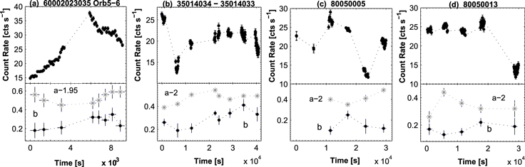
Figure 5. X-ray flux doubling/halving events (top panels), and the corresponding curvature parameter and photon index plotted vs. times (bottom panels) from the NuSTAR (plot (a)) and XRT (plots (b)–(d)) observations.
Download figure:
Standard image High-resolution imageAlong with the events shown in Figure 4, we also performed a search for 0.3–300 GeV IDVs from the contemporaneous LAT data obtained during April 11–15, showing the source's detection with (12–18)σ confidences. In the case of the April 11/12 event, an increase of the HE flux by a factor of 2.9 in 0.75 day was found. In the other cases, some time bins, obtained after splitting a day into 2–3 parts, corresponded to the source's detection below 3σ significance and/or the parameter  (the predicted number of counts based on the fitted model) was very low. Therefore, the 0.3–300 GeV IDVs from these observations cannot be credible.
We have also found two MAGIC observations with fast events (Figure 6, constructed with the data from Preziuso 2013). The VHE flux showed increases by 45%–58% in 1.1 ks and a drop by 80% in 2.1 ks on April 11/12 (Figure 6(a)). The fastest variability was a successive drop and increase by about 45%, each in about 6.7 ks on April 12/13 (Figure 6(b)). The contemporaneous X-ray data (the separate NuSTAR orbits whose time extent is several times shorter compared to the intervals between the successive observations) do not allow us to use the local cross-correlation function (LCCF, Max-Moerbeck et al. 2014) along with Monte Carlo simulations to estimate the significance of cross-correlations between the time series, and derive the value of possible time shift in the variability between these two series. The classical discrete correlation function (Edelson & Krolik 1988), used for this purpose by many authors (see, e.g., Fossati et al. 2000, 2008), is characterized by the drawback of producing spurious time lags (Max-Moerbeck et al. 2014). The source did not undergo a VHE variability during the MAGIC observation on April 14/15, while the contemporaneous NuSTAR light curve shows a flux increase by a factor of 2.1 (Figure 6(c)). Finally, we observe a tight correlation between the VHE and X-ray fluxes in the epoch of highest FACT excess rates when the latter increased by a factor of 2.3 in about 1.5 hr on April 15 (Figure 6(d)).

Figure 6. VHE IDVs of Mrk 421 (black points) along with the contemporaneous NuSTAR light curves (blue points).
Download figure:
Standard image High-resolution imageFrom the UVOT observations, we have found only two cases of UV IDVs. Namely, the UWW1-band flux showed a variability with 99.9% confidence on January 10 (a decay by 17%), and the UV flux was variable by 19%–28% in all bands on April 11/12.
3.3. Sub-hour Variability
The IDVs described in the previous subsection also consist of segments which show very fast variability within 1 hr. We have detected 37 and 56 such events from the XRT and NuSTAR observations, respectively (see Table 5 which provides a summary of these events, similar to Table 4). Among them, there were very fast events occurring within 1 ks. The top row of Figure 6 presents the light curves from the XRT observation ObsID 00080050019 (April 12/13), each lasting less than 1 ks and exhibiting a flux variability with  . After a flux increase by about 10% during the first orbit lasting 420 s (Figure 7(a)), we observe a faster drop by 23% from nearly the same flux level during the first 360 s segment of orbit 2 (Figure 7(b)). The time separation between these orbits was 3.8 ks. After fluctuations by 4%–7% during orbit 7 (lasting 840 s; (Figure 7(c))), the flux showed a brightening by 17% in the first 240 s segment of orbit 8 (starting after 4.86 ks), followed by a decay by 10% (Figure 7(d)).

Figure 7. Very fast X-ray events from the XRT (sub-figures (a)–(i)) and NuSTAR (sub-figures (j)–(l)) in Period 5. Figures 7(e)–(f) correspond to the cases when some segments of the particular orbit yield PL spectra while there are LP spectra for other segments. The values of spectral parameters are not plotted vs. time for these orbits.
Download figure:
Standard image High-resolution imageTable 5. Extract from the Summary of Subhour X-Ray Flux Variability from the XRT and NuSTAR Observations
| ObsID(s) | Obs. Dur.(ks) |

|
Bin(s) |

|
a | b |
 (keV) (keV) |
|---|---|---|---|---|---|---|---|
| (1) | (2) | (3) | (4) | (5) | (6) | (7) | (8) |
| XRT | |||||||
| 80050001 Orbit 1 | 1.60 | 5.16/12 | 120 | 6.87(0.81) | 2.81(0.02) | 0.33(0.07) | 0.06(0.04) |
| 35014034 Orbit 2 | 1.32 | 6.55/10 | 120 | 7.21(0.94) | 2.42(0.02) | 0.19(0.06) | 0.08(0.07) |
Note. The columns are the same as in Table 4.
Only a portion of this table is shown here to demonstrate its form and content. A machine-readable version of the full table is available.
Download table as: DataTypeset image
Flux fluctuations by 9%–14% within 300–720 s are also evident from the second row of Figure 7, presenting the light curves from separate orbits of ObsIDs 00035014063, 00034014065, and 00080050018 (April 14/15, 17, and 12, respectively). The other orbits of the latter observation showed a sub-hour variability, but they were longer than 1 ks (see Table 5 for their summary). Similar to Figures 7(g) and (h), the third row of Figure 7 presents the IDVs from orbits lasting 1.5–3.2 ks, and we observe a very fast variability from some small segments of the corresponding light curves. Namely, two consecutive micro-flares with increasing amplitudes and durations are evident during orbit 13 of the NuSTAR April 11/12 observation (Figure 7(j), which is a small segment from the top panel of Figure 4(a)). An increase by 16% in 660 s was recorded during the NuSTAR April 16/17 observation (orbit 7, Figure 7(k)). We observe a very fast increase by 22% in 420 s after Δt = 1 ks from the start of the ninth orbit of the same observation, and a decay by 15% occurred in the last 540 s segment of this orbit (Figure 6(l)).
Our MWL study of Mrk 421 in the period 2013 January–June shows that the source was extremely variable in X-rays both on weekly and intra-day timescales. The X-ray flares sometimes were not accompanied by a significant flaring activity in the UV and HE γ-ray parts of the spectrum.
4. SPECTRAL VARIABILITY
We performed the X-ray spectral analysis by fixing the hydrogen column density to the Galactic value  cm−2, taken from the Leiden/Argentine/Bonn Survey of Galactic HI (Kalberla et al. 2005), and using the LP model (Massaro et al. 2004, hereafter M04)

with  , the pivot energy fixed to 1 and 10 keV for the XRT and NuSTAR spectra, respectively; a, the photon index at the energy
  b, the curvature parameter; and K, the normalization factor. The values of these parameters are derived during the fit process. The location of the SED peak is given by

We extracted the spectra from separate orbits of a single observation when it was impossible to use the same source and background extraction regions for all orbits (in the case of XRT observations), or the source showed a flux variability during this observation. We used the same method even for a single orbit, when the flux varied within it, or there was no satisfactory value of the reduced chi-square for the spectrum extracted from the whole orbit (although the presence of a spectral curvature was evident).
4.1. The XRT Spectra
The results of the XRT spectral analysis performed with the LP model are provided in Table 6. The hardness ratio (HR) was calculated as a ratio of the unabsorbed 2–10 keV to 0.3–2 keV fluxes. In Table 7, we present the properties of the distribution of the parameters a, HR, and b. The peaks of the distributions are derived via the log-normal fit to the corresponding histograms (see Figure 8). The source mainly showed curved spectra, and about 80% of the values of the parameter b are included in the interval between 0.15 and 0.30 from their overall spread of Δb = 0.49 (Figure 8(a)). This parameter showed neither a correlation with the unabsorbed 0.3–10 keV model flux (Figure 9(a)), nor with the parameter a (see the corresponding discussion below) either for the data taken as a whole, or split into its separate periods. The mean value of this parameter  range from 0.20 to 0.26 for the separate periods, and its lowest values are found in Periods 4 and 5 when the source was most variable and showed the highest fluxes. The largest curvature b = 0.47 was found for the ninth segment of the fifth orbit of ObsID 00080050019 when the source showed the most violent flux variability in the XRT band. During this event, the curvature parameter varied by Δb = 0.34. As for the ObsID 00035014063 (MJD 56396.9), when the source was most hard, and the unabsorbed 0.3–10 keV flux showed its highest historical level, the curvature was low (b = 0.12–0.23), and some segments were fitted well with the simple PL model (see below). The parameter b showed only a very weak anti-correlation with the SED peak location (see Figure 9(b), and Table 8 for the Pearson correlation coefficient and corresponding p-value), although this analysis was restricted to only the spectra with
  0.80 keV (as explained below).

Figure 8. Distribution of different spectral parameters from the XRT and NuSTAR observations. The red dashed lines represent log-normal fits with the histograms.
Download figure:
Standard image High-resolution image
Figure 9. Correlation between different spectral parameters and fluxes. The XRT data are plotted with the black points, while those from NuSTAR with gray asterisks (except for Figure 9(g) where black points are used for Period 1, circles for Period 2, and gray asterisks for Period 3).
Download figure:
Standard image High-resolution imageTable 6. Extract from the Summary of the XRT Spectral Analysis with the LP Model
| ObsId | a | b |

|
K |

|

|

|

|
HR |
|---|---|---|---|---|---|---|---|---|---|
| (1) | (2) | (3) | (4) | (5) | (6) | (7) | (8) | (9) | (10) |
| 80050001 Orbit1 | 2.81(0.02) | 0.33(0.07) | 0.06(0.04) | 0.052(0.001) | 0.998/195 | −9.702(0.006) | −10.49(0.021) | −9.637(0.007) | 0.163(0.008) |
| 35014024 | 2.64(0.01) | 0.29(0.04) | 0.08(0.04) | 0.120(0.004) | 0.903/236 | −9.368(0.004) | −10.013(0.013) | −9.279(0.004) | 0.227(0.007) |
Note. The  values (Column 4) are given in keV; unabsorbed 0.3–2 keV, 2–10 keV, and 0.3–10 keV fluxes (Columns 7–9)—in erg cm−2 s−1.
Only a portion of this table is shown here to demonstrate its form and content. A machine-readable version of the full table is available.
Download table as: DataTypeset image
Table 7. Distribution of Different Spectral Parameters
| XRT | NuSTAR | |||||||
|---|---|---|---|---|---|---|---|---|
| Quant. | Min. | Max. | Peak |

|
Min. | Max. | Peak |

|
| a | 1.68 | 2.83 | 2.11 | 0.09 | 2.28 | 3.20 | 2.62 | 0.055 |
| HR | 0.159 | 1.419 | 0.450 | 0.08 | 0.239 | 1.019 | 0.546 | 0.038 |
| b | 0.09 | 0.47 | 0.19 | 0.0058 | 0.13 | 0.57 | 0.27 | 0.01 |
| Γ | 1.70 | 2.76 | 2.03 | 0.07 | 2.38 | 3.16 | 2.67 | 0.05 |

|
0.80 | 10.0 | 1.50 | 0.07 | 3.50 | 4.35 | ⋯ | ⋯ |
Download table as: ASCIITypeset image
Table 8. Correlations Between Different Spectral Parameters and Multi-band Fluxes
| Quantities | r | p |
|---|---|---|
| XRT | ||
b and 
|
−0.23(0.12) |

|
a and 
|
−0.73(0.05) |

|
 and and 
|
0.26(0.12) |

|
Γ and 
|
−0.72(0.05) |

|
HR and 
|
0.73(0.05) |

|
 and and 
|
0.87(0.03) |

|
 and and 
|
0.45(0.09) |

|
 and and 
|
0.49(0.08) |

|
 and and 
|
0.48(0.08) |

|
 and and 
|
0.95(0.02) |

|
 and and 
|
0.95(0.02) |

|
 and and 
|
0.96(0.02) |

|
 and and 
|
0.35(0.13) |

|
 and and 
|
0.55(0.10) |

|
 and and 
|
0.61(0.09) |

|
 and and 
|
0.59(0.10) |

|
| NuSTAR | ||
b and 
|
0.23(0.12) |

|
a and 
|
−0.64(0.06) |

|
Γ and 
|
−0.69(0.06) |

|
HR and 
|
0.72(0.05) |

|
 and and 
|
0.88(0.03) |

|
Note.  ,
,  , and
, and  stand for the unabsorbed UVW1, UVM2, and UVW2-band fluxes, respectively;
  is the LAT-band flux; other quantities are defined in the text and in the captions of Tables 6 and 10.
Download table as: ASCIITypeset image
As for the parameter a, it also showed a very wide range of values with Δa = 1.1 (Figure 8(b)). Its mean value from different periods varied between 2.02 and 2.64. The hardest spectra with  are found for Period 5 (
 is the mean value of the parameter a in a particular period), while the source showed very soft spectra with
  in Periods 1, 3, and 6 . The spectra with
  mostly correspond to the unabsorbed 0.3–10 keV flux values higher than 2.50 × 10⁻⁹ erg cm−2 s−1 (99.2% of which belong to Period 5), and the softest spectra with
  are found for
  = (1.36–8.97) × 10−10 erg cm−2s−1 (note that mean weighted flux value was 1.70 × 10⁻⁹ erg cm−2 s−1). The extreme values a = 1.68–1.80 correspond to the segments of orbits 3 and 4 from ObsID 00035014063 with
  =(2.79–5.81) × 10−9 erg cm−2 s−1. These facts are reflected in Figure 9(c) which shows a strong anti-correlation between a and the 0.3–10 keV flux, revealing that the source mostly followed a "harder-when-brighter" spectral trend during the 2013 January–May period. However, this trend was violated for ObsIDs 00080050018 and 00080050019 (April 12–13) corresponding to the highest X-ray states during Flare 1 (see the bottom panel of Figure 4(a) from MJD 56394.0 and the second panel of Figure 4(b)). Period 5 exhibits the largest variations of the photon index by Δa = 0.87. On the IDV timescales, the largest variability by Δa = 0.54 corresponds to the April 11–12 event, and this parameter showed a variability on timescales less than 1 ks (see Section 5.2). In contrast to other periods, this parameter varied only by Δa = 0.19 in Period 3 while the unabsorbed 0.3–10 keV flux varied by a factor of 3. Note that the opposite spectral evolution is evident during the flux increase phase of the IDV presented in Figure 5(b).
The position of the SED peak had a very wide range between  = 0.005 ± 0.008 keV and
  keV. However, the values
  0.80 keV derived from the X-ray spectral analysis are systematically higher than those obtained from the contemporaneous broadband SEDs via the fit with the LP function (introduced by Landau et al. 1986)

i.e., the intrinsic position of the synchrotron SED peak is poorly constrained by the XRT observation in that case. Therefore, these  values should be considered as upper limits to the intrinsic ones (see Kapanadze et al. 2014, 2016a). We have not used them when searching for the correlations of
  with other spectral parameters (or fluxes) and for the construction of the histogram presented in Figure 8(c). Note that 80% of the values with
  keV are found in the soft X-ray part of the spectrum (
 keV), and the distribution of this parameter exhibits a prominent peak at
  keV. No significant correlation was found between
  and the 0.3–10 keV flux, and there is only a very weak positive correlation between
  and the 2–10 keV flux (Figure 9(d)). The largest values of this parameter are derived for the segments of ObsID 00035014063. However, for the spectra extracted from some segments of orbits 2–4 and for those from all segments of orbit 5 of this observation, the curvature parameter had values below
  , and the fit with the LP model did not give better statistics than that with the simple PL
  , where Γ is the photon index throughout the observation band. Therefore, the latter model was chosen for these spectra (see Table 9 for the results). The same was true for some segments from ObsID(000350140)64,65 (April 16–17) and several XRT observations corresponding to the target's low brightness states in Periods 1, 2, 3, and 6. The parameter Γ also had a broad range ΔΓ = 1.06 (see Figure 8(d)), and 48% of the PL spectra had a photon index below the value Γ = 2 (during the flares in Period 5), while those from quiescent states were very soft with
  . Similar to the parameter a, Γ showed a strong anti-correlation with the 0.3–10 keV flux (Figure 9(e)).
Table 9. Extract from the Summary of the XRT Spectral Analysis with a Simple PL Model
| ObsId | Γ | K |

|

|

|

|
HR |
|---|---|---|---|---|---|---|---|
| (1) | (2) | (3) | (4) | (5) | (6) | (7) | (8) |
| 80050001 Orbit1 | 2.74(0.05) | 0.062(0.002) | 1.114/64 | −9.69(0.006) | −0.404(0.012) | −9.614(0.005) | 0.193(0.006) |
| 35014028 Orbit1 | 2.79(0.03) | 0.053(0.001) | 0.877/121 | −9.663(0.008) | −10.333(0.02) | −9.579(0.007) | 0.214(0.011) |
Note. The quantities are given in the same units as in Table 6.
Only a portion of this table is shown here to demonstrate its form and content. A machine-readable version of the full table is available.
Download table as: DataTypeset image
The parameter HR also had a wide range ΔHR = 1.26 (Figure 8(e), including the values derived from the spectra fitted with the PL model). Its highest values HR = 0.723–1.419 are derived for the observations with the 0.3–10 keV count rates above 100 cts s−1 during Flares 1 and 2. As for the low X-ray states in different periods with  cts s−1, we obtained HR = 0.164–0.347. Although this parameter shows a strong positive correlation with the 0.3–10 keV flux during 2013 January–May (confirming the general dominance of a "harder-when-brighter" evolution of the flares; see Figure 9(f)), the correlation strength was unequal in different periods; while it was the strongest in Period 1, we do not observe a correlation with 99% confidence in Periods 2 and 3. Flares 1–3 ranged from r = 0.66 ± 0.06 (Flare 1) to r = 0.87 ± 0.03 (Flare 1; see Figure 9(g)). From Flare 1, all the segments of ObsID 00080050019 and most of those from ObsID 00080050018 with
  3.3 × 10⁻⁹ erg cm−2 s−1 do not show a significant correlation with the 0.3–10 keV flux, producing outliers from the whole sample in the lower right parts of Figures 9(f) and (g). Note that these data points show a progressively horizontal trend with increasing energy.
4.2. The NuSTAR Spectra
The NuSTAR observations also mostly showed curved spectra (see Table 10). Similar to Paliya et al. (2015), we fixed the pivot energy to 10 keV when using the LP model for them. On average, these spectra had larger values and a wider range of the parameter b compared to those from the XRT band (see Table 10 and Figure 8(f)). In contrast to the latter, a curvature of the NuSTAR spectra showed a very weak, although statistically significant, correlation with the unabsorbed flux from the same spectral range (see Figure 9(a), upper sample depicted by red points). This correlation was the case with IDVs observed on April 11/12 (after  0.55 day from the start of the NuSTAR observation) and April 16/17 (Figures 4(a) and (f)) with r = 0.35–0.45. However, the sample of the NuSTAR data points corresponding to
  = 2.4 × 10⁻⁹ erg cm−2 s−1 does not exhibit a significant correlation with the 3–79 keV flux, in contrast to those corresponding to the lower fluxes. This mainly happened for the observations performed during April 12–15 (see Figures 4(b) and (d)). We cannot draw conclusions about the existence of a correlation between the parameters b and
  (observed for the XRT spectra) since only 6% of the spectra show the synchrotron SED peak above 3.50 keV, below which the SED peak is poorly constrained and should be considered as an upper limit to the intrinsic value. The largest value of
  was 4.35 ± 0.85 keV from the first 300 s segment of orbit 6 from the April 14/15 observation. Note that most of the segments from orbits 6–9 of this observation yielded
  keV, and the contemporaneous XRT observation also showed the highest values of this parameter then.
Table 10. Extract from the Summary of the NuSTAR Spectral Analysis with the LP Model
| ObsId | a | b |

|
K |

|

|

|

|
HR |
|---|---|---|---|---|---|---|---|---|---|
| (1) | (2) | (3) | (4) | (5) | (6) | (7) | (8) | (9) | (10) |
| 6000202306 | 3.12(0.02) | 0.23(0.04) | 0.04(0.03) | 0.20(0.01) | 1.053/421 | −10.121(0.002) | −10.623(0.012) | −10.002(0.003) | 0.315(0.009) |
| 60002023010 | 3.08(0.02) | 0.31(0.05) | 0.18(0.08) | 0.28(0.01) | 0.902/403 | −9.998(0.002) | −10.474(0.011) | −9.873(0.003) | 0.334(0.009) |
Note. The quantities are given in the same units as in Table 6, except for fit norm (column 5) which is given in units of 10−3.  ,
,  , and
, and  stand for the unabsorbed 3–10 keV, 10–79 keV, and 3–79 keV fluxes, respectively.
Only a portion of this table is shown here to demonstrate its form and content. A machine-readable version of the full table is available.
Download table as: DataTypeset image
The photon index at 10 keV also had a wide range of values (Δa = 0.95) but significantly higher values compared to its counterpart from the XRT spectra, where 97% of its values are found in the interval a = 2.3–3.0 (Figure 8(g)). The source showed a "harder-when-brighter" spectral evolution in this case as well, and the photon index showed an anti-correlation to the 10 keV flux (see Figure 9(c)). This fact is evident from Figures 4(a)–(f) where the time evolution of the parameter a along with the 3–79 keV count rate during the extreme IDVs of the April 11–17 period are presented (except for Figure 4(c) where this trend is not clearly seen). The softest spectra with  belong to the lowest brightness states, while the values
  are derived for the segments corresponding to highest brightness states during Flares 1–3 in Period 5. Two sub-samples: (1) the values derived from the segments of orbits 5–9 of the April 14/15 observation and (2) those from the last two orbits of ObsID 60002023025 (MJD 56393.1) and subsequent two NuSTAR observations (corresponding to the peaks of Flare 2 and Flare 1, respectively) show a weaker correlation with the flux compared to other observations and produce two outliers from the scatter plot (see the upper sample in Figure 9(c) depicted by red points). On intra-day timescales, the largest variability of this parameter by Δa = −0.54 in 15.25 hr was observed on April 2. It also underwent an extreme variability with Δa = 0.48 in 19 hr on April 11/12 (Figure 4(a), second panel), and showed a variability on sub-hour timescales (see Figures 4(g)–(l)).
Finally, about 9% of the NuSTAR spectra did not exhibit a spectral curvature (corresponding to any brightness state of the source), and we fitted them with the simple PL, yielding the 3–79 keV photon index Γ = 2.38–3.16 (see Table 11), with a strong anti-correlation with the 3–79 keV flux. A large range of ΔHR = 0.78 was also seen for the 10–79 keV to 3–10 keV flux ratio (Figure 8(h)) whose strong positive correlation with the unabsorbed 3–79 keV band (Figure 9(f), the sample depicted by red points) also confirms a "harder-when-brighter" spectral evolution in this band.
Table 11. Extract from the Summary of the NuSTAR Spectral Analysis with a Simple PL Model
| ObsId | Γ | K |

|

|

|

|
HR |
|---|---|---|---|---|---|---|---|
| (1) | (2) | (3) | (4) | (5) | (6) | (7) | (8) |
| 60002023002 | 3.14(0.02) | 0.110(0.004) | 1.039/208 | −10.481(0.005) | −10.924(0.037) | −10.345(0.010) | 0.361(0.031) |
| 60002023004 | 3.16(0.02) | 0.078(0.003) | 1.118/232 | −10.647(0.004) | −11.091(0.029) | −10.514(0.008) | 0.360(0.024) |
Note. The quantities are given in the same units as in Table 6.
Only a portion of this table is shown here to demonstrate its form and content. A machine-readable version of the full table is available.
Download table as: DataTypeset image
Our spectral study shows that the X-ray spectra of Mrk 421 were mainly curved during 2013 January–May with broad ranges of photon index, curvature parameter, HR, and synchrotron SED peak location, all of which exhibit an extreme variability on different timescales.
5. DISCUSSION
In this section, we discuss the results from the MWL flux variability and X-ray spectral study of Mrk 421 along with those published to date.
5.1. Flux Variability
Our timing analysis of the Swift-XRT observations of Mrk 421 during 2013 January–June has revealed the 0.3–10 keV flux variability, from fluctuations observed within 1 ks to strong flares on weekly timescales. Although B16 mentioned the January–March period as an epoch of "quiescent states" for Mrk 421, this conclusion was based on the results from the NuSTAR observations in this period when they were sampled relatively sparsely and the source was found in a faint X-ray state also in the 0.3–10 keV band. In the case of relatively densely sampled XRT observations, we have revealed five consecutive X-ray flares with flux increases by a factor of 2.6–7.2 with a large range of 0.3–10 keV count rates of 7–85 cts s−1 (with 1 minute time bins).
Generally, the source exhibited an increasing value of the quantity  from IDVs for the longer-term flares in different periods (see Tables 3–5). This property, referred to as "red noise" (see Aleksic et al. 2015a), is one of the well-known properties of blazars. Using the power spectral density technique for well-sampled long-term light curves, different authors showed the presence of larger variability at smaller frequencies/longer timescales in the form
  with spectral index α between 1 and 2 (see Abdo et al. 2010; Chatterjee et al. 2012 etc.). For the MWL campaign on Mrk 421 in 2009, Aleksic et al. (2015a) derived the range α = 1.3–2.0 from the VHE to radio frequencies.
The flux variability also showed increasing power toward higher frequencies in the synchrotron part of the spectrum that is evident from Figure 10 where the  values from each band, calculated using all the available data obtained during the whole January–June period, are plotted versus frequency. The
  value from the 0.3 to 300 GeV band, calculated via the fluxes from daily-binned LAT data, is almost two times smaller than those from the X-ray bands. As for the
  value from the MAGIC observations, it could be larger, since we used data above the 200 GeV threshold for Periods 1–4, while the only available MAGIC data from Period 5 (where the source exhibited the strongest variability and largest VHE fluxes) correspond to
  GeV, and the MAGIC observations do not cover the whole epoch of giant X-ray outbursts when a very strong VHE flare was revealed by FACT. Nevertheless, the largest fractional variability is found from the FACT observations corresponding to detections with at least 3σ significance. Note that similar results for Mrk 421 were reported by Aleksic et al. (2015a) and Bartoli et al. (2016). This property was suggested as an indication that the electron energy distribution is most variable at the highest energies (within the one-zone SSC scenario; see Aleksic et al. 2015a). PKS 2155–304 and 1ES 1959+650 showed increasing variability power across the whole electromagnetic spectrum where
  was related to the photon energy as
  with m = 0.043–0.08 (Kapanadze et al. 2014, 2016a).

Figure 10. Fractional rms variability amplitude as a function of frequency from the MWL observations of Mrk 421 in the 2016 January–June period.
Download figure:
Standard image High-resolution image5.2. Interband Cross-correlations
The unabsorbed soft 0.3–2 keV flux showed a strong positive correlation with the hard 2–10 keV flux (see the first plot of Figure 9(h)). In each period, the corresponding light curves followed each other closely, and no significant time shift between them is evident on daily timescales. However, the hard flux varied with a larger amplitude than the soft one in each period (see Table 3), leading to strong spectral variability during these events (see Section 5.3 for the corresponding discussion). This difference was especially large in Period 5 when the 0.3–2 keV flux varied by a factor of 7.6, while we observe a variability by a factor 30.9 in the 2–10 keV band. A similar situation is also evident from the NuSTAR observations where the 10–79 keV flux shows a stronger variability compared to the 3–10 keV one.
During the half-year of data presented here, the X-ray flares were mainly accompanied by their counterparts in the UV and γ-ray bands. From past observations, similar cases were reported by different authors for Mrk 421. Buckley et al. (1996) reported a correlated TeV/X-ray/UV/optical variability in 1995 April–May. The X-ray and TeV intensities were well correlated on timescales of hours in 1998 April (Maraschi et al. 1999). The source showed strong variations in both X-ray and γ-ray bands in 2001 March, which were highly correlated (Fossati et al. 2008). Acciari et al. (2011) reported X-ray spectral hardening with increasing flux levels, often correlated with an increase of the source activity in the TeV flux in 2006–2008. During the MWL campaigns in 2009 January–June and 2010 March, Aleksic et al. (2015a, 2015b) observed a positive correlation between VHE and X-ray fluxes with zero time lag. These results indicate that the X-ray and VHE emissions were co-spatial and produced by the same population of HE particles.
The 0.3–10 keV flux showed weak positive correlations with the UV and 0.3–300 GeV fluxes (see Figures 9(i) and (j), respectively), while we observe a stronger correlation between the UV and HE γ-ray fluxes (see Table 8 and Figure 9(k); we provide scatter plots only for the  band here, since the fluxes from the UV bands show very strong positive correlations with each other with r = 0.95–0.96). This result can be explained by the stronger connection between the UV and HE γ-ray emissions via the IC scatter of synchrotron photons, while the contribution of X-ray photons to the 0.3–300 GeV band should be significantly smaller for Mrk 421 in the period under discussion. Tramacere et al. (2009) (hereafter T09) suggested a possible positive correlation between the UV and MeV/GeV-band fluxes via the effect of Klein–Nishina suppression in the IC process, leading to the UV photons being upscattered most efficiently at GeV energies by electrons radiating in the X-ray. Macomb et al. (1995) reported strong contemporaneous TeV and X-ray flares in 1994 May, while no significant GeV flare was seen. During the ARGO-YBJ observations in 2008–2012, the X-ray flux was clearly correlated with the VHE flux, while the HE one showed only a partial correlation with them. The radio and UV fluxes were weakly or not correlated with the X-ray and γ-ray fluxes (Bartoli et al. 2016). During the MWL campaign in 2009 January–June, Aleksic et al. (2015a) observed an overall anti-correlation between optical/UV and X-rays, spreading over a large range of time lags, and proposed three scenarios for these events: (1) the optical/UV and the X-ray/VHE emissions were dominated by emission from two distinct and unconnected regions with different temporal evolutions of their corresponding particle populations; (2) a two-component (high- and low-energy) particle population, in which the low and high-energy particles have a different but related long-term temporal evolution; and (3) a global long-term change in the efficiency of the acceleration mechanism, producing an electron energy distribution that could shift the entire synchrotron bump to higher/lower energies—if this mechanism causes the index of the electron population to get harder, the emission at the rising segment of the synchrotron SED (radio-UV) would decrease, while that on the decreasing segment (X-rays) would increase. The latter scenario seems to be the most plausible for Period 2 when the UV light curves showed a permanent decay and subsequent low UV state, while we observe an X-ray flare in this epoch. Meanwhile, the 0.3–300 GeV flux was also close to its lowest level during the January–June period, and this fact is also in favor of the connection between the UV and HE γ-ray emissions. A similar situation was observed in the beginning of Period 4 as well, and in the epochs of giant X-ray flares in Period 5. The X-ray flare detected with MAXI in 2013 June was also not accompanied by its HE counterpart.
In the first half of Period 4 and on April 14/15, uncorrelated X-ray and TeV variabilities were observed that have also occurred in the past. The MWL campaign in 2002 December–2003 January revealed a rather loose correlation between the X-ray and TeV fluxes, although there was also a very strong X-ray flare with flux varying by a factor of 7 within 3 days not accompanied by a comparable TeV counterpart (Rebillot et al. 2006). The TeV flux reached its peak days before the X-ray flux during the giant flare in 2004 that was impossible to explain via the standard one-zone SSC model, and Blazejowski et al. (2005) suggested this as an instance of an "orphan" TeV flare. Acciari et al. (2011) also found high X-ray states, not accompanied by TeV flaring and vice versa in 2006–2008. A weak correlation between X-ray and VHE flares with a time lag of ∼1 day was revealed in 2009 November (Shukla et al. 2012).
5.3. Flux Variability on Intra-day Timescales
The duty cycle (DC, i.e., the fraction of the total observation time during which the object displays a variability; see Romero et al. 1999) of the IDVs detected at 3σ confidence was 83% for the XRT observations of Mrk 421, and the source was always variable during the NuSTAR observations, except for the three cases when the exposure was very short (78–441 s). The higher DC of Mrk 421 from NuSTAR observations than that from the XRT campaign can be explained as being due to the aforementioned increasing variability power with frequency. However, this result can be partially related to the fact that the NuSTAR observations were significantly longer and denser sampled compared to the XRT ones. The longest XRT observation without an IDV had an exposure of 2.67 ks distributed over a 6.64 ks interval (two orbits, performed on May 11 when the source decayed to its quiescent state). The observations without IDVs mainly belong to the lower X-ray states. Although these observations are mostly shorter than 1.1 ks, a non-detection of IDVs cannot simply be related to their shortness. We have revealed seven cases from the XRT observations when an IDV was observed within 1 ks, and they represent the fastest X-ray flux variability reported to date. Note that they all belong to the epochs of Flares 1 and 2 with  cts s−1. The majority of longer X-ray IDVs are also observed in higher brightness states, especially during Flares 1–3. It is therefore easier to explain these events in the framework of a shock-in-jet scenario (interaction of a propagating shock front with jet inhomogeneities; Sokolov et al. 2004) rather than via other instability mechanisms, e.g., those occurring near the event horizon of a central black hole which should be more conspicuous when the source is faint since the fast but low amplitude variations will not be overwhelmed by the steady shocked flow emission (Mangalam & Wiita 1993). However, we also revealed two IDVs occurring within 1 ks in the lower brightness epochs (from the NuSTAR observations). Therefore, the possibility of alternative scenarios for a very fast flux variability in some epochs cannot be excluded. The sub-hour IDVs are found during VHE observations of Mrk 421 (in Period 5), but they are not as fast and dramatic as those detected from X-ray observations, or very fast VHE events reported during past 20 years (see below).
The extreme X-ray IDVs presented in Figures 4 and 5 show flux doubling and halving timescales  hr and
  = 2.30–2.40 hr in the NusTAR band, calculated via the equation
  (Saito et al. 2013) from the segments of the light curves incorporating flux changes by a factor 2 and more. These ranges are wider in the XRT band where
  hr and
  hr, but this fact can be related to the more dense sampling of the NuSTAR light curves compared to the 0.3–10 keV ones where the time intervals between the successive XRT orbits are generally significantly larger compared to the duration of the orbits themselves. Paliya et al. (2015) reported the fastest flux doubling timescale of 14.01 ± 5.03 minutes from the NuSTAR observations of April 10–19, although this result seems to be obtained from one the short segments of the light curves which show a large slope but a flux increase factor less than 2 (followed by an interruption in the observation).
In past studies, very fast flux variability was reported several times for this source. During the two dramatic TeV outbursts on 1996 May 7, the first one had a doubling time of about 1 hr, and the flux increased above the relatively quiescent value by more than a factor of 50. In the second outburst, which lasted approximately 30 minutes, the flux increased by a factor of 20–25 (Gaidos et al. 1996). A sub-hour variability with two overlapping flares of even shorter durations was reported by Cui (2004) from the RXTE-PCA observations of a high X-ray state in 2001. The source showed rapid VHE variability with the flux doubling time as short as 20 minutes in 2001 January–April (Aharonian et al. 2002). Blazejowski et al. (2005) found two very fast X-ray micro-flares during ∼20 minutes with substantial sub-structures, implying variability on even shorter timescales, and no counterparts were apparent at TeV energies (RXTE-PCA observations in 2004 February). Other events with a short rise or decay time of 1 ks were also detected. Aleksic et al. (2010) reported the VHE flux doubling time of 36 ± minutes from the MAGIC observation of 2006 April 29 ( GeV).
GeV).
While the fractional variability amplitudes of X-ray IDVs longer than 1 hr (presented in Table 4) do not show show a clear correlation with the corresponding count rates (Figure 9(l)), the faster events, observed on sub-hour timescales, exhibit a weak anti-correlation with the flux (r = 0.33 ± 0.13; Figure 9(m)). Note that an anti-correlation between the fractional amplitude and the flux was also reported by Zhang et al. (2006) and Mangalam & Wiita (1993) that was suggested to be an indication of a strong non-stationary origin of the X-ray variability. However, as we see from Figure 9(m), the sub-sample of the sub-hour IDVs observed in higher X-ray states do not follow this trend, in contrast to those occurring in lower states, and this fact can be related to different underlying instability mechanisms for these two sub-samples.
Our target is much more variable on intra-day timescales compared to 1ES 1959+650 and PKS 2155–304 with DC = 22.55%–48% for the IDVs with 99.9% significance (Kapanadze et al. 2014, 2016a).
5.4. Spectral Variability
5.4.1. Ranges of Spectral Parameters
The source also underwent an extreme spectral variability in the 0.3–10 keV band, and exhibited an evolution from the softest spectrum with photon index at 1 keV a = 2.83 ± 0.02 in a quiescent state to a very hard one with a = 1.68 ± 0.01 during Flare 2. From the previous X-ray spectral studies of Mrk 421, even harder spectra with a = 1.63–1.67 were reported by T09 from the XRT observations performed during 2006 April–July, while the softest spectrum of this period corresponds to a = 2.10, and 98% of the spectra from this period showed  . Note that the source reached its highest historical unabsorbed 0.3–10 keV flux of 3.41 × 10⁻⁹ erg cm−2 s−1 in 2006 April, but significantly larger fluxes were observed during the highest states during Flares 1 and 2, and the value
  = 6.70 × 10⁻⁹ erg cm−2 s−1 was recorded on April 15. During the 2008 June flare, the source was as hard as a = 1.65 (Donnarumma et al. 2009). The hardest spectra with a = 1.34–1.45 are reported by Ravasio et al. (2004) from the two XMM-Newton observations in 2002 November–December. Note that these observations did not correspond to a very bright state of Mrk 421 since the 2–10 keV fluxes of (3.35–4.21) × 10−10 erg cm−2 s−1, extracted from them, were significantly smaller than those observed in the highest X-ray states during Periods 4 and 5. The LP fit yielding a = 1.16–1.50 for another two spectra from Ravasio et al. (2004) was not satisfactory, and these values of the photon index are not credible. In 2005 March–July, the source exhibited significantly softer spectra with a = 2.10–2.58 (Tramacere et al. 2007). The BeppoSAX observations of 1997–2000 showed a = 1.70–2.54 (M04). Therefore, our study reveals the historical softest states of Mrk 421.
5.4.2. Timing of Spectral Parameters
In Figure 9(c), the scatter plots a– and a–
 (where a is the photon index at 10 keV in the latter case) clearly exhibit the dominance of a "harder-when-brighter" spectral evolution of Mrk 421 during flares in the 0.3–79 keV energy range. However, they also show a significant scatter in the data points, indicating that the evolutions of the flares were different from each other due to different underlying physical conditions (T09). As noted in Section 4, this is especially evident from the sub-samples corresponding to the extreme IDVs observed in the peaks of Flares 1 and 2 which do not show a significant anti-correlation, and produce almost horizontal outliers from the scatter plots.
During the past campaigns, a "harder-when-brighter" spectral evolution of Mrk 421 was reported by several authors (see, e.g., T09, Acciari et al. 2011; Aleksic et al. 2015a). The opposite evolution has not been reported to date for this source, and we detected it only on one occasion for a segment of the 0.3–10 keV observation with an IDV.
Unprecedented high brightness states and very fast IDVs at the peaks of Flares 1 and 2 allowed us to detect a spectral variability within the 1 ks interval. Namely, a hardening by Δa = 0.12 in 470 s (Figure 7(i)), and a softening by Δa = 0.10 in 400 s (Figure 7(h)) were observed in these epochs. Note that the detection of very fast spectral variability events from the NuSTAR observations were limited due to higher errors compared to the XRT ones. On timescales larger than 1 ks, we have found a softening by Δa = 0.18 in 4.7 ks (Figure 5(d)) and a hardening by Δa = 0.28 in 11.8 ks (Figure 4(f), bottom panel). The source also showed very fast spectral changes during past campaigns. Namely, Brinkmann et al. (2005) reported spectral variations on timescales as short as 500–1000 s from the XMM-Newton observations in 2002–2004. The 3–20 keV photon index hardened by ΔΓ = 0.18 within 1.6 hr and softened by ΔΓ = 0.20 in the same time in 2000 February (Krawczynski et al. 2001).
5.4.3. The Occurrence of PL Spectra
Our study revealed that about 13% of all XRT spectra were characterized by  , and the LP model did show a better fit compared to the PL one. We therefore have used the latter model for further analysis, which showed a very broad range Γ = 1.70–2.76 for the photon index through the 0.3–10 keV band. Note that the aforementioned largest value of unabsorbed 0.3–10 keV flux during 2013 January–June is derived from the second 250 s segment of orbit 5 from ObsID 00035016063, fitted well with the PL model.
Generally, the PL spectra from the NuSTAR and XRT observations are from the same epochs. We have revealed the following trend for the simultaneous XRT and NuSTAR segments with curved spectra: during the higher X-ray states, the values of the parameter b obtained from the 3–79 keV band, is mostly larger by  than those derived from the XRT band. This difference decreases with X-ray flux, and when the NuSTAR band count rate is less than about 1.60 cts s−1, we observe the opposite situation. In the low X-ray states, we have found four cases when the XRT spectrum was curved, while its NuSTAR counterpart fitted the PL model well.15
This fact could be explained via the increasing contribution of the IC photons to the higher-energy part of the 3–79 keV band with decreasing X-ray flux that, eventually, would lead to a decrease the curvature in this band compared to the XRT one. Furthermore, B16 reported b = −0.2 ± 0.1 for the NuSTAR spectrum extracted from ObsID 60002023002 (January 2) corresponding to one of the lowest brightness state of Mrk 421 in this band. Our spectral analysis of the same spectrum has revealed that the LP and PL fits yield practically the same statistics, and we do not observe an increasing trend of the residuals with higher energy in the case of the LP fit, similar to those cases reported by Zhang et al. (2006) from the XMM-Newton observations of PKS 2155–304 when the residuals exhibited a continuously increasing trend with energy starting from
than those derived from the XRT band. This difference decreases with X-ray flux, and when the NuSTAR band count rate is less than about 1.60 cts s−1, we observe the opposite situation. In the low X-ray states, we have found four cases when the XRT spectrum was curved, while its NuSTAR counterpart fitted the PL model well.15
This fact could be explained via the increasing contribution of the IC photons to the higher-energy part of the 3–79 keV band with decreasing X-ray flux that, eventually, would lead to a decrease the curvature in this band compared to the XRT one. Furthermore, B16 reported b = −0.2 ± 0.1 for the NuSTAR spectrum extracted from ObsID 60002023002 (January 2) corresponding to one of the lowest brightness state of Mrk 421 in this band. Our spectral analysis of the same spectrum has revealed that the LP and PL fits yield practically the same statistics, and we do not observe an increasing trend of the residuals with higher energy in the case of the LP fit, similar to those cases reported by Zhang et al. (2006) from the XMM-Newton observations of PKS 2155–304 when the residuals exhibited a continuously increasing trend with energy starting from  keV. The appearance of a negative value of the parameter b for the aforementioned NuSTAR spectrum is presumably related to the excess counts around 40 keV after which the residuals show a decreasing trend. Therefore, we cannot explain them as due to the contribution made by the IC photons. Therefore, we have chosen an LP fit to this spectrum. Note that similar excesses are found in other 3–79 keV spectra from the low X-ray states fitted well with PL or LP models. Furthermore, none of the NuSTAR spectra, corresponding the observations with 3–79 keV count rate below 1.60 cts s−1, show a trend of continuously increasing residuals with energy, and the one-zone SSC fit of B16 with the broadband SEDs constructed with data obtained simultaneously with some of these NuSTAR observations do not give an indication about the significant IC contribution to the 3–79 keV band either. Therefore, the aforementioned differences in curvature strength between the XRT and NuSTAR spectra can be rather related to the positive correlation between the parameter b and the 3–79 keV flux, while a similar correlation is not found in the XRT band.
Note that 2013 January–June was not the only epoch when the PL spectra of Mrk 421 were also observed (along with the curved spectra). Although T09 present the results of the LP fit with all the spectra from the 2006 April to July epoch, we have checked that for most of these spectra with  , the LP fit does not give better statistics than the PL fit. PL spectra with Γ = 1.52–1.60 in the 0.6–10 keV band were reported by Ravasio et al. (2004), and Γ = 1.97–2.90 in the 4–15 keV by Rebillot et al. (2006). The presence of PL spectra for some other HBLs were reported by Kapanadze et al. (2016a) (1ES 1959+650), Kapanadze et al. (2014) (PKS 2155–304), Tramacere et al. (2007) (1H 1100−230, PKS 2005–489, 1ES 2344+514), and Massaro et al. (2008) (1ES 0347–121, PKS 0548–322 etc.).
5.4.4. Spectral Curvature
Curved spectra are known to arise both for synchrotron and IC radiation from electron distributions following the LP distribution with energy (Massaro et al. 2011). According to M04, the LP spectrum of accelerated electrons, formed by some statistical mechanism, is related to the fact that the probability  of a particle's subsequent acceleration at step i is related to its Lorentz factor
  (i.e., to its energy) as
  , where g and q are constants. If
  , the probability of subsequent acceleration becomes gradually lower as the energy increases, and this may cause the establishment of an LP energy spectrum of relativistic electrons. This effect may occur in a medium where the electrons are confined by a magnetic field with a confinement efficiency decreasing with increasing gyroradius (M04). We suggest that this effect was probably stronger for electrons emitting photons in the 10–79 keV band via the synchrotron mechanism during the period presented here, than for those emitting in the 0.3–10 keV band. It is possible that the q parameter did not have the same values during different brightness states, and it became larger with the increasing 3–79 keV flux that led to the appearance of a positive correlation between the flux and curvature parameter. However, this effect did not work in the highest X-ray states during Flares 1 and 2 when a positive correlation between b and the flux is not evident.
If we merge the results from both NuSTAR and XRT bands, the parameter b has a range of 0.09–0.57. The results of the LP fit of the X-ray spectra of Mrk 421 published to date show that  is very rare for this source (reported mainly by M04 for the 1997–1999 epoch), and most of the spectra show low curvatures, i.e., broad synchrotron SEDs which are expected in the case of an efficient stochastic acceleration of emitting electrons in the jets of TeV-detected HBLs (Massaro et al. 2011). Although we observe an anti-correlation between b and
  as predicted within the stochastic scenario when a mono-energetic or quasi-mono-energetic electron injection in the acceleration zone occurs (T09), it is very weak, and this fact may indicate that the assumption about the mono-energetic or quasi-mono-energetic injection was not valid during the X-ray flares observed in 2013 January–May, and more complex injection scenarios are necessary for the stochastically accelerated electrons. Furthermore, this fact may be related the the "contamination" of a stochastic acceleration of the electrons by other acceleration or cooling mechanisms. The energy-dependent acceleration probability process (EDAP, M04) predicts a positive correlation between the parameters a and b that was not observed for Mrk 421 in the period presented here, in contrast to its BeppoSAX observations in 1997–1998 (M04).
Similar to the photon index, the parameter b sometimes also showed a very fast variability. Its decays by Δb = 0.12–0.16 in 350–900 s (Figures 7(c)–(d)) and increases by Δb = 0.27–0.34 in 700–900 s (Figures 7(i) and (l)) are revealed by our detailed spectral study.
Sinha et al. (2015) performed a joint spectral analysis of XRT and NuSTAR spectra grouped within 13 segments of Period 5, and obtained a = 1.61–2.39, b = 0.27–0.46, and  keV. It was concluded that these spectra originated from the LP electron spectrum, although a broken PL or a PL with an exponentially falling electron distribution cannot be ruled out. They also showed that the X-ray flares should be caused by a separate electron population which does not contribute significantly to the radiation at lower energies. However, our modeling of the broadband SEDs from the April 11–15 period clearly showed better fits for the PL+LP electron spectrum, and the electrons contributing to the X-ray band followed the LP distribution (see Section 5.4).
5.5. Spectral Hysteresis
Analysis of hysteresis patterns in the HR–flux plane is useful for drawing conclusions about the interplay between electron acceleration ( ), synchrotron cooling (
 ), and flux variability (
 ) timescales. In this plane, one may observe (Cui 2004):
(a) a clockwise (CW) loop, if  , or
, or  . In this case, the spectrum becomes steeper in the declining phase and harder in the brightening phase, indicating that variations of hard X-rays always lead to those in the soft X-rays both during the increase and decrease of the brightness of the source (Takahashi et al. 1996). Figure 11(a) presents the spectral evolution during the X-ray flare observed with XRT in Period 2 in the HR–flux plane. We observe two subsequent CW loops here, hinting at a possible soft lag during this event. The possibility of a hard lag is evident from the accompanying plot where the normalized unabsorbed soft 0.3–2 keV and hard 2–10 keV fluxes are plotted versus time. We see that the hard flux had its first peak before MJD 56325, while the peak of the soft one followed this moment. Similar to the cases reported in Section 3.3, our sparsely sampled data (one data point extracted from a separate XRT pointing whose time extent is several times shorter compared to the intervals between the successive observations) do not allow us to use the LCCF technique, and derive the value of a soft lag. Therefore, the aforementioned possible soft lag should be treated with caution. A CW-type spectral evolution is also evident from the IDV observed with XRT on March 4/5 (Figure 11(b)), where the 2–10 keV peak is seen at 6.36 ks after the start of the observation, while the 0.3–2 keV one probably occurred during the subsequent 0.6 ks interval. We also observe a much faster increase of the hard X-ray flux compared to the soft one, 22 ks after the start of the pointing. The CW loops are also seen for the Period 3 flare and for the IDVs on February 17, March 10, and April 18 observed with XRT, as well as for the IDVs revealed via NuSTAR on April 13/14, April 15/16, April 16/17 (orbits 5–6), and April 11/12 (orbit 26).

Figure 11. Examples of different types of spectral hysteresis patterns from the flares on different timescales along with soft fluxes (gray asterisks; 0.3–2 keV for XRT, 3–10 keV for NuSTAR) and hard fluxes (blue points; 2–10 keV for XRT, 10–79 keV for NuSTAR) plotted versus time: CW (upper row), CCW (middle row), both CW and CCW (lower row). The fluxes are normalized to their minimum values reached during the particular flare. The light curved for hard fluxes are shifted arbitrarily for better resolution.
Download figure:
Standard image High-resolution image(b) a CCW loop, when  . Information about the occurrence of a flare propagates from lower to higher energies, as particles are gradually accelerated, while the decay of the flare could be dominated by particle escape effects, which can be assumed to be achromatic, and we therefore should observe a hard lag (Ravasio et al. 2004). The source showed a CCW loop during the IDV observed with XRT on March 11 (Figure 11(c))—the hard flux still shows an increase during the first 5.6 ks of the pointing (followed by a decay), while the soft flux was already decreasing. The soft 3–10 keV flux underwent a permanent increase during the first 2.55 ks of orbit 9 from the NuSTAR observation on April 14 (with a possible minimum before the start of this orbit), while the hard 10–79 keV flux showed a decay during the first 1.05 ks, followed by an increase, and it reached a maximum just after a soft peak (Figure 11(d)). The CCW loops are also evident in the XRT IDVs on January 15, January 20, March 11, April 14/15, and April 19.
The source showed a change from CW-type evolution into the opposite one and vice versa during some longer-term and intra-day flares. The most dramatic was the NuSTAR observation on April 11/12 (Figure 11(e)). During the first six orbits lasting 28.3 ks, we observe a CCW-type evolution. The soft 3–10 keV flux decayed during all these orbits, while the 10–79 keV one started a decay after the third orbit. Afterwards, there was a linear increase lasting 45 ks which was significantly faster and stronger in the 10–79 keV band, and we observe a CW-type evolution. The next 42.5 ks interval was characterized by three consecutive CCW-type episodes, which were related to minor fast X-ray flares with increasing amplitudes, superimposed on this dramatic IDV. According to T09, a flux increase with a rapid spectral hardening can serve as an indication of the appearance of a new flaring component in the hard band. Therefore, a flux increase by a factor of 8 during this extreme event can be related to contributions from several flaring components. As for the IDV on April 15/16 (Figure 11(f)), we observe a transition from the CCW (a possible hard 2–10 keV lag within the first 6.3 ks interval since the observation start) into CW-type evolution (a possible soft lag in the interval Δt = 23–30 ks). Changes in the spectral hysteresis also occurred over the course of the most powerful X-ray flare in Period 5 (although the CW and CCW loops are not perfectly drawn), as well as during Periods 1, 4, and 6, the IDV on April 12/13, orbit 4 of ObsID 00080050018 (April 12) and ObsID 00035014065 (April 17) observed with XRT, and orbit 9 from the NuSTAR pointing on April 16/17.
Our study of the hysteresis patterns in the spectral evolution of Mrk 421 shows that the extreme spectral variability observed in 2013 January–May was related to the very complex interplay between the acceleration and cooling timescales of emitting particles, and each longer-term and fast X-ray flare had a different characterization in terms of the competition between these timescales. Since hysteresis probes the timescale of the cooling processes as a function of energy, Figure 11 reveals that some flares had a cooling time acting faster at higher energies, and this situation is consistent with the dominance of synchrotron cooling, since its timescale is shorter at higher energies (Falcone et al. 2004). According to T09, this behavior is probably due to the flaring component starting in the hard X-ray band, and implies that the driver of those flares was a rapid injection of very energetic particles rather than a gradual acceleration, when a CCW-type evolution and a hard lag is expected. Our HR–flux diagrams showed many cases when the spectrum started to become harder, while the 0.3–10 keV or the 3–79 keV flux was still decreasing, which may indicate propagation of the new injection from the hard band, as the soft band is still decreasing (T09). These cases were seen during both longer-term and fast flares, underlining a complex character of X-ray variability on a wide range of timescales.
From past X-ray studies, CW-type spectral evolution of Mrk 421 was reported by T09, Takahashi et al. (1996, 2000), Cui (2004), Ravasio et al. (2004), and Rebillot et al. (2006), and the opposite one by the same authors and Zhang (2002). T09 also presented several cases when the source showed a transition from a CW-type evolution into the opposite one and vice versa during 2006 April–July, demonstrating that 2013 January–June was not the only period when the physical factors responsible for the spectral variability varied in a very complex manner.
5.6. Spectral Energy Distribution
5.6.1. The Location of Synchrotron SED Peak
Our spectral study of Mrk 421 has revealed a very wide range of the parameter  during 2013 January–April. The spectral analysis of the XRT observations performed in the epochs of the lower X-ray state revealed the presence of a synchrotron SED peak at frequencies as low as a few eV, and the corresponding
  values should be even lower since those smaller than about 0.8 keV are upper limits to the intrinsic ones. For the observations with PL X-ray spectra, we constructed broadband SEDs using the available MWL data, and performed a fit with Equation (4) to find the position of the synchrotron SED. In this way, we revealed that the corresponding SED peak values also have a very wide range from far-UV energies to beyond 10 keV. Figure 12 presents the 0.3–10 keV SEDs from observations with the PL spectra which showed a very high hardness ratio HR = 1.337–1.419, and their fit with Equation (4) exhibits the presence of the SED peak between 11.40 ± 2.10 keV and 18.50 ± 2.50 keV. Note that the
  values derived from Figures 12(a)–(c) show an increasing trend with the larger 0.3–10 keV flux which is in agreement with the positive correlation between these quantities reported in Section 4. However, these values must be treated with caution since no observational data are available at the peaks of the corresponding SEDs, and we consider them as upper limits to the intrinsic peak positions.

Figure 12. X-ray SEDs corresponding to  keV.
keV.
Download figure:
Standard image High-resolution imageNote that the aforementioned spectra with synchrotron SED position, possibly exceeding the 10 keV threshold, and the largest value of the parameter  (see Section 4.1) belong to the epoch of Flare 2, and, therefore, this flare is characterized by a shift of the SED peak location by
  1.50. However, this spectral variability is significantly less extreme than that exhibited by another HBL source Mrk 501 during a dramatic X-ray flare in 1997 April when the position of the synchrotron SED moved from 0.94 keV to beyond 100 keV (Pian et al. 1998; Tavecchio et al. 2001). While the presence of the synchrotron peak beyond 100 keV was firmly established during that event, it could not be constrained from above because of BeppoSAX's lack of sensitivity beyond 100 keV (see Tavecchio et al. 2001). Therefore, a shift of the SED peak location
  in this case which is significantly larger than that shown by Mrk 421 in 2013 April. Furthermore, the highest-energy synchrotron peak shown by the latter source during Flare 2 is about an order of magnitude smaller than that observed for Mrk 501 in 1997 April. This source also showed a large shift in the
  parameter from 0.79 ± 0.08 keV to 21.98 ± 2.81 keV during strong and prolonged X-ray activity in 2014 March–October, observed by Swift-XRT (B. Kapanadze et al. 2016, in preparation). Note that 95% of these spectra showed
  keV, while only 10% of the curved XRT spectra of Mrk 421 from the epochs of Flares 1 and 2 (which were much stronger than those of Mrk 501 in 2014) are found in this energy range. Therefore, we conclude that there should be some physical "agent" responsible for "inhibiting" very large
  values during strong X-ray flares in Mrk 421, which must be much weaker or absent in Mrk 501.
T09 reported many cases with  keV and even
  keV from the 2006 April–July observations of Mrk 421. However, these results are obtained for those spectra not exhibiting a significant curvature (discussed in Section 5.2). For example, this fact is evident for the spectra extracted from the orbits (or from their separate segments) of ObsID 00030352014. However, the presence of the spectral curvature is significant for some of those spectra, which locate the synchrotron SED peak beyond 10 keV (e.g., those from ObsID 00219237000 corresponding to the highest X-ray state in this period). These results, along with those presented in this paper, show that the synchrotron SED of Mrk 421 exhibits a very large shift in its position, providing evidence for dramatic changes in the physical conditions in this source, since the SED peak location is related to the jet physical parameters as
  (T09), where
  is the peak of the distribution
  . Furthermore, the dependence between
  and
and  (or between
  and
and 
 and
and  are the peak height and the isotropic luminosity at
  ) in the form
  can be used to draw a conclusion about the physical factor (variations in the average electron energy/number, magnetic field, beaming factor) which makes the main contribution to the observed spectral variability (depending on the values of the parameter α; see Tramacere et al. 2007). However, we have not found a correlation between these parameters16
neither for the whole January–May period, nor for any X-ray flare, that leads to the suggestion that the spectral variability in Mrk 41 was very complex, and it could not be defined by a single factor. In contrast to our result, Massaro et al. (2008) found a correlation between
can be used to draw a conclusion about the physical factor (variations in the average electron energy/number, magnetic field, beaming factor) which makes the main contribution to the observed spectral variability (depending on the values of the parameter α; see Tramacere et al. 2007). However, we have not found a correlation between these parameters16
neither for the whole January–May period, nor for any X-ray flare, that leads to the suggestion that the spectral variability in Mrk 41 was very complex, and it could not be defined by a single factor. In contrast to our result, Massaro et al. (2008) found a correlation between  and
and  with rlog = 0.67 (the linear correlation coefficient between the logarithms of these parameters) for Mrk 421 from the BeppoSAX, XMM-Newton, and Swift observations in 1996–1997.
5.6.2. Modeling of a Broadband SED
Figure 13 presents the broadband SEDs constructed via the MWL data obtained along with five MAGIC observations performed in April 11–15. The VHE spectral points are taken from Preziuso (2013). While the UVOT, XRT, and NuSTAR data are strictly simultaneous with the MAGIC ones, we used the daily-binned LAT data (centered on the MAGIC observations) in order to achieve the extraction of a few spectral points with 3σ confidence in the 0.3–300 GeV energy range. The OVRO data were not available for each day of this period, and we have used the mean  values from the April 11–15 period for them. Note that the source did not show radio variability with 3σ confidence in this epoch. We performed modeling of these SEDs in the framework of the one-zone SSC scenario via the online code developed by A. Tramacere17
, and described in detail by Tramacere et al. (2011), T09, and Massaro et al. (2006). In this model, a spherical emission region of radius R is filled with a relativistic electron population (N electrons per cm3), moving down the jet with a bulk Lorentz factor
values from the April 11–15 period for them. Note that the source did not show radio variability with 3σ confidence in this epoch. We performed modeling of these SEDs in the framework of the one-zone SSC scenario via the online code developed by A. Tramacere17
, and described in detail by Tramacere et al. (2011), T09, and Massaro et al. (2006). In this model, a spherical emission region of radius R is filled with a relativistic electron population (N electrons per cm3), moving down the jet with a bulk Lorentz factor  . The magnetic field B in the emission region is randomly oriented, and emitted radiation is Doppler-boosted by δ =
  , where
  and θ, the angle between the jet axis and the observer's line of sight. In all cases, the best fit was obtained for the distribution of the emitting electrons as an LP function plus a PL low-energy segment, defined as

with  , the energy at which the PL distribution turns into the LP one; s, the spectral index at the reference energy
  and r, the spectral curvature. The results of the modeling are presented in Table 12, yielding the size of the emission region R = (1.7–2.9) × 1017, moving with
  and
and  1
1 9 toward the observer.18
The relativistic electrons with N = 2.1–2.2 cm−3, embedded in the magnetic field B = 0.07–0.12 G, have an energy range with lower and upper limits of
9 toward the observer.18
The relativistic electrons with N = 2.1–2.2 cm−3, embedded in the magnetic field B = 0.07–0.12 G, have an energy range with lower and upper limits of  , and
, and  , respectively. Below
  = (0.7–1.7) × 105, they revealed the PL distribution with energy, and above this threshold the LP one with r = 1.4–1.6, s = 1.95–2.40. The fits yield the observed synchrotron peak frequency
  =(1.41–5.24) × 1017 Hz, and the SSC peak frequency
  = (1.00–6.22) × 1025 Hz.

Figure 13. Broadband SEDs of Mrk 421 from the epoch of Flares 1 and 2 constructed via the simultaneous data from OVRO, UVOT, XRT, NuSTAR, LAT, and MAGIC. The dashed blue lines represent a simple one-zone SSC model discussed in Section 5.4.
Download figure:
Standard image High-resolution imageTable 12. The Results of the Broadband SED Modeling
| Quant. | Apr 11 | Apr 11/12 | Apr 12/13 | Apr 13/14 | Apr 14/15 |
|---|---|---|---|---|---|
| R(1016 cm) | 1.70 | 1.70 | 1.70 | 2.00 | 2.90 |
| B(Gauss) | 0.12 | 0.10 | 0.10 | 0.10 | 0.07 |
| N(cm−3) | 2.20 | 2.10 | 2.10 | 2.20 | 2.20 |

|
30 | 40 | 40 | 35 | 30 |
| δ | 30.2 | 29.0 | 29.0 | 29.83 | 30.2 |
 (×102) (×102) |
5.0 | 2.8 | 1.8 | 2.8 | 3.5 |
 (×108) (×108) |
1.3 | 1.8 | 1.0 | 1.6 | 1.6 |
 (×104) (×104) |
7.0 | 6.9 | 7.0 | 6.0 | 17.0 |
| r | 1.60 | 1.60 | 1.40 | 1.48 | 1.55 |
| s | 2.40 | 2.10 | 1.95 | 2.20 | 2.40 |
 (1017 Hz) (1017 Hz) |
1.49 | 2.33 | 3.38 | 1.41 | 5.24 |
 (1025 Hz) (1025 Hz) |
1.00 | 3.92 | 6.22 | 2.13 | 2.72 |
Download table as: ASCIITypeset image
For the modeling of the broadband SEDs of Mrk 421, constructed from past MWL campaigns, a similar distribution of electrons with energy was successfully used by T09 and Acciari et al. (2011), although we have obtained significantly larger values of  and a broader range of electron energies. The physical parameters of the emission region would be more extreme for very fast events described in Section 3.3 (especially for the parameter δ which should be very high (≳50) in order to avoid a severe pair production of TeV photons with synchrotron radiation; see Paliya et al. 2015), or for the events with
  keV presented in Figure 12 (the April 12–17 period), but we cannot construct broadband SEDs for them due to the absence of strictly simultaneous spectral points in the HE and VHE bands. T09 also found one occasion when a broadband SED of our target was best described via the pure LP distribution. Other attempts at modeling were successful when adopting a simple PL or a PL with one or two breaks by B16, Aleksic et al. (2012, 2015b), Pian et al. (2014), Abdo et al. (2011), etc. Therefore, we conclude that the electron distribution with energy varied from epoch to epoch in Mrk 421 due to changes in the underlying acceleration processes.
6. CONCLUSIONS
We have presented the results of X-ray observations of the HBL source Mrk 421 performed by Swift-XRT and NuSTAR during 2013 January–June. It exhibited a strong long-term variability of 0.3–10 keV and 3–79 keV fluxes with maximum-to-minimum ratios of 22 and 95, respectively, in about 3 months. The flux variability was characterized by changing in its amplitude and minimum flux level from flare to flare. The very high values of the ratio  in both bands were related to the unprecedentedly strong X-ray outbursts during April 11–17 when the 0.3–10 keV count rate exceeded the level of 200 cts s−1 for19
the first time since the start of the Swift observations of Mrk 421, and it became one of the brightest sources on the X-ray sky. The unabsorbed hard 0.3–2 keV flux showed a strong positive correlation with the hard 2–10 keV flux, and no significant time shift between them is evident on daily timescales. However, the hard flux generally varied more strongly, and the ratio R was four times larger compared to that in the soft band. A similar situation was also evident from the NuSTAR observations where the 10–79 keV flux showed a stronger variability compared to the 3–10 keV one.
in both bands were related to the unprecedentedly strong X-ray outbursts during April 11–17 when the 0.3–10 keV count rate exceeded the level of 200 cts s−1 for19
the first time since the start of the Swift observations of Mrk 421, and it became one of the brightest sources on the X-ray sky. The unabsorbed hard 0.3–2 keV flux showed a strong positive correlation with the hard 2–10 keV flux, and no significant time shift between them is evident on daily timescales. However, the hard flux generally varied more strongly, and the ratio R was four times larger compared to that in the soft band. A similar situation was also evident from the NuSTAR observations where the 10–79 keV flux showed a stronger variability compared to the 3–10 keV one.
During the half-year period for which we present data, the X-ray flares were sometimes accompanied by those in the UV and γ-ray bands, which favors a one-zone SSC scenario. However, the UV and HE flares were much weaker compared to their X-ray counterpart during April 11–17 (as well as in some other periods), and they generally showed a significantly stronger correlation with each other than to the X-ray fluxes. This result confirms earlier suggestions about the possible stronger connection between the UV and HE fluxes due the effect of Klein–Nishina suppression on the IC process, leading to more effective upscattering of UV photons at GeV energies by electrons radiating in the X-ray band. Moreover, the UV and HE fluxes showed a decay and subsequent low states in Period 2 when the source showed a flaring activity in X-ray and VHE bands. A similar situation was seen in the epochs of the giant X-ray outbursts in Period 5. These facts can be explained via the global long-term change in the efficiency of the acceleration mechanism, shifting the entire synchrotron bump to higher energies. The VHE emission showed a stronger correlation with the X-ray fluxes, and the FACT observations revealed a very strong VHE flare during April 11–17. However, we have found uncorrelated X-ray and VHE variability on two occasions—in the first half of Period 4 and during the 2.2 hr MAGIC observation on the night of April 14/15 when increasing X-ray activity was accompanied by decaying and constant TeV fluxes, respectively.
The source also showed an unprecedentedly high variability on intra-day timescales, and its duty cycle ranged from 83% to almost 100% in different X-ray bands. IDVs exhibited flux doubling and halving timescales  hr and
  hr, respectively. The fastest events were observed during April 11–17, especially in the highest X-ray states (Flares 1 and 2) when the flux varied by 4%–23% within 300–840 s. In this period, the source exhibited the most extreme IDVs since the start of X-ray observations of Mrk 421.
During 2013 January–April, the source also underwent the most extreme X-ray spectral variabilities ever reported for this source. The spectra were mainly curved and fitted well with the LP model. The location of the synchrotron SED peak moved from a few eV to ∼10 keV. The photon index at 1 keV and curvature parameter values had ranges a = 1.68–2.83 and b = 0.09–0.47, respectively, and varied along with the 0.3–10 keV flux on different timescales from a few weeks down to intervals shorter than 1 ks. The curvature parameter showed an even larger range of 0.13–0.57 in the 3–79 keV band. The dominance of broad synchrotron SEDs, i.e., low values of the parameter b, and the observed b– anti-correlation is more easily explained via the effective stochastic acceleration of electrons producing X-ray photons, and this result is in agreement with the earlier suggestion about the more effective stochastic acceleration of electrons in jets of TeV-detected HBLs compared to TeV-undetected objects. We have not found the correlation
  during X-ray flares observed in 2013 January–May, and since it is based on the assumption of mono-energetic or quasi-mono-energetic injection of particles in the emission zone, this mechanism should not be valid for our target, and more complex injection scenarios are necessary for the stochastically accelerated electrons.
The scatter plots clearly demonstrated the dominance of a "harder-when-brighter" spectral evolution during the flares on different timescales. However, a significant scatter in the data points indicates that the evolution of the flares was different due to different underlying physical conditions. This conclusion is confirmed by a detailed study of spectral hysteresis patterns for these events which exhibited CW (flare with a cooling time acting faster at higher energies, to be related to a rapid injection of very energetic particles rather than a gradual acceleration) and CCW (a gradual acceleration with possible hard lag) loops, and the transitions between them in the HR–flux plane. These cases were seen as often during longer-term, as during fast flares, underlining the complex character of X-ray variability on a wide range of timescales.
We conclude that Mrk 421 is one of the most extreme HBLs with a very complex, unpredictable timing/spectral variability, exclusively strong X-ray flares in some epochs, and that further intensive MWL campaigns will be very useful for gaining a deeper understanding of the AGN phenomenon and the physics of relativistic jets.
B.K., S.K., and L.T. acknowledge Shota Rustaveli National Science Foundation and Ilia State University for the grant FR/377/6-290/14. PR acknowledges the contract ASI-INAF I/004/11/0. This research has made use of the XRTDAS software, developed under the responsibility of the ASDC, Italy, and the data from the OVRO 40 m monitoring program which is supported in part by NASA grants NNX08AW31G and NNX11A043G, and NSF grants AST-0808050 and AST-1109911. We thank the FACT Collaboration for providing their analysis results publicly, and appreciate very much their long-term monitoring initiative which provides precious input for MWL studies. This research has made use of the online SED_tool developed by Andrea Tramacere. This research has made use of the NuSTAR Data Analysis Software jointly developed by the ASI Science Data Center (ASDC, Italy) and California Institute of Technology (Caltech, USA). This research has made use of the MAXI data provided by RIKEN, JAXA, and the MAXI team. B.K. acknowledges a Roland and Eileen Weiser Professional Development Award issued by Weiser Center for Europe & Eurasia for a short-term scientific stay at the University of Michigan (Ann Arbor, USA) and thanks the staff of the Department of Astronomy for its hospitality. Finally, we thank the anonymous referee for the very useful comments and suggestions that helped to improve the quality of the paper.
Footnotes
- 5
- 6
- 7
- 8
According to T. Mihara (2016, private communication).
- 9
- 10
The UVM2 light curve follows them very closely, and we do not present it here.
- 11
- 12
There were no FACT observations on the April 13/14 night when the VHE peak in Figure 1(g) was observed with MAGIC.
- 13
In this period, Mrk 421 was observed by MAGIC and FACT only from the April 11/12 night when the source was in its increasing VHE state. No MAGIC data are available for the days before Period 5. FACT observed the source from the April 13/14 night, and it was detected with less than 3σ confidence each day during April 4–9.
- 14
- 15
A joint fit of these XRT and NuSTAR spectra with PL shows clear trends in the residuals for the energies
, i.e., this model does not fit the XRT spectrum. - 16
We calculated
according to M04. - 17
- 18
We used different values of the angle θ during the fitting process in each case. However, the best fits were obtained when θ was close to 1
9. - 19
The corresponding unabsorbed 0.3–10 keV flux
erg cm−2 s−1 for our target, depending on the spectral shape during the particular observation.

