


Abstract
The Apache Point Observatory Galactic Evolution Experiment (APOGEE), one of the programs in the Sloan Digital Sky Survey III (SDSS-III), has now completed its systematic, homogeneous spectroscopic survey sampling all major populations of the Milky Way. After a three-year observing campaign on the Sloan 2.5 m Telescope, APOGEE has collected a half million high-resolution (R ∼ 22,500), high signal-to-noise ratio (>100), infrared (1.51–1.70 μm) spectra for 146,000 stars, with time series information via repeat visits to most of these stars. This paper describes the motivations for the survey and its overall design—hardware, field placement, target selection, operations—and gives an overview of these aspects as well as the data reduction, analysis, and products. An index is also given to the complement of technical papers that describe various critical survey components in detail. Finally, we discuss the achieved survey performance and illustrate the variety of potential uses of the data products by way of a number of science demonstrations, which span from time series analysis of stellar spectral variations and radial velocity variations from stellar companions, to spatial maps of kinematics, metallicity, and abundance patterns across the Galaxy and as a function of age, to new views of the interstellar medium, the chemistry of star clusters, and the discovery of rare stellar species. As part of SDSS-III Data Release 12 and later releases, all of the APOGEE data products are publicly available.
Export citation and abstract BibTeX RIS
1. Introduction
1.1. Galactic Archaeology Surveys
Modern astrophysics has taken two general observational approaches to understand the evolution of galaxies. On the one hand, increasingly larger aperture telescopes, on the ground and in space, give access to the high-redshift universe and offer "low-resolution" snapshots of ever earlier phases of galaxy evolution. On the other hand, increasingly efficient, multiplexing photometric and spectroscopic instrumentation, often on smaller, workhorse telescopes, has made possible enormous, definitive surveys of nearby galaxies, yielding a "high-resolution (HR)" view of the present state of these systems. These data can be tested against "end state" predictions for the growth of large structures in the universe to provide critical constraints on cosmological models—so-called "near-field cosmology". These two observational approaches—overviews of global properties at high redshift versus more detailed information at low redshift—provide complementary information that must be accommodated by evolutionary theories.
The highest-granularity information about galaxy evolution is provided by stars in our own Milky Way, whose present spatial distributions, ages, chemistry, and kinematics contain fossilized clues to its formation. Guided by detailed models for the chemical and dynamical evolution of stellar populations, critical telltale signatures and correlations within the above observables provide constraints on the model predictions for physical quantities that cannot be observed directly, such as the history of star formation, the early stellar initial mass function (IMF), and the merger history of Galactic subsystems. This "Galactic archaeology" remains the principal basis by which models for the formation and chemodynamical evolution of the Milky Way and analogous systems are formulated and refined. The vast literature on Milky Way stellar populations as tools for understanding Galactic evolution has been reviewed in the past by, e.g., Gilmore et al. (1989), Majewski (1993), and Freeman & Bland-Hawthorn (2002), and more recently by Ivezić et al. (2012), Rix & Bovy (2013), and Bland-Hawthorn & Gerhard (2016).
These efforts are of course greatly aided by access to expansive, carefully designed, homogeneous, and precise databases of properties for stellar samples that span large regions of the Galaxy and include all of the principal stellar populations. Modern archetypes of such databases are large photometric surveys like the Two Micron All-Sky Survey (2MASS; Skrutskie et al. 2006) and the Sloan Digital Sky Survey (SDSS; York et al. 2000). Over the past decade, these photometric catalogs have been widely exploited for insights into the nature of the Milky Way and probing the complexities of Galactic structure—e.g., halo substructure (e.g., Majewski et al. 2003; Rocha-Pinto et al. 2004; Belokurov et al. 2006; Grillmair 2009), satellite galaxies (e.g., Willman et al. 2005; Belokurov et al. 2007), the warp of the disk (e.g., López-Corredoira et al. 2002; Reylé et al. 2009), and the still unresolved, composite anatomy of the bulge (e.g., Robin et al. 2012), which includes the recently found X-shaped feature (e.g., McWilliam & Zoccali 2010; Nataf et al. 2010) and one or more central bars (e.g., Hammersley et al. 2000; Alard 2001; Cabrera-Lavers et al. 2007). Follow-on, low- and medium-resolution (MR) spectroscopic programs provide additional dynamical discrimination of, and context for, these structures as well as general information on their chemical makeup (e.g., mean metallicities and, in some cases, an additional dimension of chemistry, such as [α/Fe]); these broad brushstrokes represent an important step in characterizing stellar populations and constraining galactic evolution models.
Meanwhile, HR stellar spectroscopy has become an increasingly indispensable tool for providing the necessary detail to discriminate galaxy evolution models. Accurate multi-element chemical abundances provide insight into the stellar IMFs, and histories of star formation and chemical enrichment of stellar populations, which, in turn, fuel ever more sophisticated galactic dynamical and chemodynamical models (e.g., Chiappini et al. 2001, 2003; Sellwood & Binney 2002; Abadi et al. 2003; Bournaud et al. 2009; Schönrich & Binney 2009; Minchev & Famaey 2010; Bird et al. 2013; Minchev et al. 2013, 2014; Kubryk et al. 2015). Coupled with orbital information derived from precise radial velocities, these data probe the role of dynamical phenomena such as large-scale dissipative collapses, mergers, gas flows, bars, spiral arms, dynamical heating, and radial migration.
Conventional echelle spectroscopy programs to deliver HR spectroscopic data useful for Galactic archaeology demand substantial resources, often on the world's largest telescopes. Consequently, while heroic efforts have been devoted to surveying stars in a wide variety of environments—including, e.g., dwarf spheroidals, globular clusters, the Magellanic Clouds, tidal streams, and the Galactic bulge—until very recently the solar neighborhood was the only region for which multiple hundreds or thousands of observations had been assembled for "Galactic field stars" (e.g., Edvardsson et al. 1993; Bensby et al. 2003; Fuhrmann 2004; Venn et al. 2004; Nissen & Schuster 2010; Soubiran et al. 2010; Adibekyan et al. 2012, 2013; Bensby et al. 2014). These studies traditionally relied on kinematically selected samples to harvest from the nearby stars of accessible apparent brightnesses a broad spread of stellar ages and population classes. For stellar populations not represented in the solar neighborhood, like the Galactic bulge, and for in situ studies of field stars outside of the solar neighborhood, HR observations are only now generating samples with hundreds of stars. In the inner Galaxy where foreground dust obscuration is a formidable challenge, many previous samples were concentrated to a handful of low extinction sight lines, such as Baade's Window. Unfortunately, the aggregate of these piecemeal collections of spectroscopic data, heterogeneously assembled, can give a biased and incomplete view of the Milky Way.
Truly comprehensive evolutionary models for the Milky Way must be informed and constrained by statistically reliable, complete, or at least unbiased Galactic archaeology studies, which require the construction of large, truly systematic, and homogeneous chemokinematical surveys covering expansive volumes of the Milky Way and sampling all stellar populations, including, in particular, those dust-obscured inner regions where the bulk of the Galactic stellar mass is concentrated. A number of ambitious "Galactic archaeology" spectroscopic surveys that aim to fill this need (1) have been previously undertaken, such as RAVE (Steinmetz et al. 2006), SEGUE-1 (Yanny et al. 2009), SEGUE-2 (Rockosi et al. 2009), and ARGOS (Freeman et al. 2013), (2) are currently underway, such as LAMOST (Cui et al. 2012), Gaia/ESO (Gilmore et al. 2012), GALAH (Zucker et al. 2012), and Gaia (Perryman et al. 2001), (3) or are envisaged, e.g., those associated with the WEAVE (Dalton et al. 2014), 4MOST (de Jong et al. 2014), and MOONS (Cirasuolo et al. 2014) instruments. Although each of these surveys focuses on large samples of ≳100,000 stars, all of the past and ongoing endeavors are based on optical observations and are therefore strongly hampered by interstellar obscuration in the Galactic plane (Figure 1, bottom); this makes it challenging to sample significant numbers of stars within the very dusty regions of the Milky Way that are both central to constraining formation models and encompass most of the Galactic stellar mass (and some projects, like the RAVE, SEGUE, and GALAH surveys, specifically avoid low Galactic latitudes). Therefore, with optical wavelength surveys, it is challenging to assemble a systematic census having comparable or sufficient representation of all Galactic stellar populations and across wide expanses of the Galactic disk and bulge.

Figure 1. APOGEE in the context of other Galactic archaeology surveys, past, present, and future. The top panel shows the number of Milky Way stars, observed or anticipated, as a function of survey resolution. For those surveys with at least a resolution of R = 10,000, the bottom panel shows the expected nominal depth of the survey for a star with  in the case of no extinction (right end of arrows) and in the case of
  (left end of arrows). In both panels, already completed surveys are shown in black, ongoing surveys in dark gray, and planned surveys in light gray. For surveys with multiple resolution modes, data in the top panel are plotted separately for high resolution (HR), medium resolution (MR), and/or low resolution (LR). For the Gaia/ESO survey, data for the "Inner Galaxy" and "Halo" subsamples are shown separately as well. "Gaia-RV" includes Gaia HR spectra of enough S/N to deliver radial velocities, whereas "Gaia" indicates only those with S/N high enough for abundance work. For Gaia, we adopted
  from Jordi et al. (2010), assuming
  sample numbers were taken from http://www.cosmos.esa.int/web/gaia/science-performance.
Download figure:
Standard image High-resolution imageWhile other surveys, such as BRAVA (Rich et al. 2007), ARGOS (Freeman et al. 2013), and Gonzalez et al. (2011) aim to fill at least part of this void by specifically focusing on the Galactic bulge, they utilize target selection criteria that differ from those of surveys of other parts of the Milky Way, which makes it difficult to generate a holistic picture of stellar populations and their potential connections. Moreover, apart from GALAH and the Gaia/ESO survey, these other studies are limited to MR spectroscopy (R < 10,000; Figure 1), and so they are unable to provide reliably the kind of detailed elemental abundance information that is now a key input to the models, while at the same time the moderate velocity precisions can limit their sensitivity to more subtle, second-order dynamical effects (e.g., perturbations by spiral arms and the bar, dynamical resonances, velocity-coherent moving groups and streams).
1.2. APOGEE: Basic Architecture and Motivations
In contrast to previous and ongoing surveys, the Apache Point Observatory Galactic Evolution Experiment (APOGEE) in Sloan Digital Sky Survey III (SDSS-III) was designed to tackle the fundamental problem of galaxy formation through the first large-scale, systematic, precision chemical and kinematical study specifically optimized to include the exploration of the "dust-hidden" populations in the Milky Way. As planned, APOGEE aimed to build a database of HR (R ∼ 22,500), near-infrared (NIR; 1.6 μm H-band) spectra for over 105 stars—predominantly red giant branch (RGB) and other luminous post-main-sequence stars—across the Milky Way, but with particular emphasis on obtaining significant representation from heavily dust-obscured parts of the Galactic disk and bulge. Operationally, this plan, now successfully executed, exploits several key advantages:
- a.NIR observations profit from a selective extinction many times lower—for the H-band, a factor of 6 in magnitudes (i.e., a factor of 250 times in flux) than at visual wavelengths.
- b.HR spectra provide the chemical abundance and radial velocity precision needed for constraining Galactic evolutionary models and, in the H-band, sample lines of numerous elements up to and including the iron peak and for which non-LTE departures are typically small.
- c.Collectively, RGB stars, and asymptotic giant branch (AGB) and red supergiant (RSG) stars are good tracers of the disk, bulge, and halo; together, they sample populations of all ages and metallicities, and are luminous in the NIR. Meanwhile, the high sky density of these stellar types—combined with the large, 3° diameter Sloan 2.5 m telescope field of view (FOV) and high throughput, multifiber plugplate handling system—allows the simultaneous observation of several hundred targets at a time, and thousands per night.
Together, these advantages translate into a Milky Way survey trade-space "sweet spot" that permits efficient, high resolution, NIR spectroscopic study of large numbers of stars that are not easily accessible to optical programs, and enables a consistent database of stellar spectra to be assembled across all Galactic stellar populations, from the inner bulge to the more distant Galactic halo. Thus, with APOGEE, it is possible for the first time to explore and compare with great statistical significance the chemokinematical character of all Milky Way stellar subsystems using the same set of chemical elements and line transitions represented in data of uniformly high quality that has been gathered, processed, and analyzed identically.
1.3. High Level Science Goals
The principal scientific goals of APOGEE, which together provide a broad but integrated approach to furthering our understanding of galaxy evolution, are:
- a.To measure high-precision abundances for multiple elements in
 stars across the Galaxy, and derive distributions of these chemical properties to constrain Galactic chemical evolution (GCE) models. Among the target elements are the preferred GCE tracers and most common metals—i.e., carbon, nitrogen, and oxygen—as well as other metals with particular sensitivity to the star formation history (SFH) and the IMF of stellar populations.
 - b.To derive high-precision kinematical data useful for constraining dynamical models for the disk, bulge, bar, and halo, and for discriminating substructures within these components.
- c.To access the often ignored, dust-obscured inner regions of the Galaxy, and for the observed stars in these regions derive the same data as are available for other, more accessible stellar populations, which will also be included in the survey; furthermore, by collecting large survey samples, provide statistically reliable measures of chemistry and kinematics in dozens of Galactic zones (R, θ, Z) at the level currently available in the solar neighborhood.
- d.To contribute to explorations of the early Galaxy by inferring the properties of the earliest stars, thought to reside or to have resided within a few kiloparsecs of the Galactic center (Tumlinson 2010). This can be achieved either by detecting them directly if they survive to the present day, or (more likely) by measuring their nucleosynthetic products in the most metal-poor stars that do survive.
- e.To achieve a dramatic (more than two orders of magnitude) leap in the total number of available high resolution, high signal-to-noise ratio (S/N) infrared stellar spectra, which will enable substantial advances in stellar astrophysics, GCE modeling, and dynamical modeling of the Milky Way.

Among the more specific issues that APOGEE addresses are:
- a.Completing the first systematic determination of the 3D chemical abundance distribution—for numerous elements—across the Galactic disk, determining the Galactic rotation curve, and examining correlations between abundances and stellar kinematics at all disk radii.
- b.Determining the distribution functions of chemical abundances for a variety of elements in the bulge, bar(s), and inner disk, and probing correlations between abundances and kinematics there, with the goal of investigating the physical mechanisms that connect these structures and determining the origin(s) of the bulge.
- c.Establishing the nature of the Galactic bar(s) and spiral arms and their influence on the disk through detailed assessment of abundances and velocities of stars in and around them.
- d.Assessing the properties that discriminate the thin and thick disks to clarify the nature and origin of the latter.
- e.Drawing a comprehensive picture of the chemical evolution of the Galaxy via the placement of strong constraints on the IMF and star formation rates of the bulge, disk, and halo as a function of position and time.
- f.Searching for and probing the chemistry and dynamics of low-latitude substructures in both the disk and halo, whether from dynamical resonances or the accretion of satellites.
- g.Investigating the kinematics and chemistry of the Galactic halo and its substructure, and using them to assess the relative contribution of accreted versus stars formed in situ.
- h.By reference to other available optical, near-IR, mid-IR and radio data, exploring the interstellar medium, mapping the Galactic dust distribution, and constraining variations in the interstellar extinction law.
- i.By combining spectroscopic data with the detailed information on stellar structure provided by asteroseismology surveys, deriving accurate ages for Galactic field stars, which provide key timestamps for the exploration of all manner of Galactic evolutionary phenomena.
- j.Through the marriage of accurate stellar parameters and detailed chemical compositions from APOGEE with accurate asteroseismological data, providing fundamental constraints on models of the structure of stellar interiors, opening doors to progress in important areas of stellar physics.
1.4. Goals of this Paper
The goal of the present paper is to give a broad overview of the APOGEE survey, with particular focus on the scientific motivations and technical rationale that led to the instrument and survey design choices (Section 2). The "birds-eye" descriptions of the APOGEE project given here are at a level intended to give the potential user of APOGEE data sufficient background to understand the basic structure of the instrument (Section 3) and survey (Section 4), how the data were collected (Section 5) and processed (Section 6), and what the data look like and how they may be accessed (Section 8). We also summarize how the survey met its intended goals (Section 7), further illustrated via several science demonstrations (Section 7.4). The latter also introduce some of the variety of applications to which APOGEE data may be directed. Based on the success of the APOGEE project, a new collaboration has been formed to expand upon this initial survey via the APOGEE-2 project; these and related future efforts are discussed briefly in Section 9.
This paper is a primer for those interested in a general understanding of the overall structure of the APOGEE survey. For more details on particular aspects of the survey, users are encouraged to consult a series of focused technical papers that address various specific elements of the survey, the software and algorithms used to produce the publicly released databases, and post-survey assessments of the calibration and accuracy of the data (Table 1). These papers and other survey documentation are described further in Section 8.4. Online information describing the data release file formats and available online tools for data visualization and download may be found at http://www.sdss.org.
Table 1. APOGEE Survey Technical Papers
| Topic | Reference |
|---|---|
| Spectrograph | J. C. Wilson et al. (2017, in preparation) |
| Target Selection | Zasowski et al. (2013) |
| Data Reduction Pipeline | Nidever et al. (2015) |
| Stellar Atmosphere Models | Mészáros et al. (2012) |
| Stellar Spectral Libraries | Zamora et al. (2015) |
| APOGEE Line List | Shetrone et al. (2015) |
| Tests of the APOGEE Line List | Smith et al. (2013) |
| Stellar Parameters and Chemical | |
| Abundances Pipeline (ASPCAP) | García Pérez et al. (2016) |
| ASPCAP Calibration for | |
| Data Release 10 (DR10) | Mészáros et al. (2013) |
| Overview of Data Release 12 (DR12) | |
| APOGEE data | Holtzman et al. (2015) |
| Kepler Asteroseismology Collaboration | Pinsonneault et al. (2014) |
| CoRoT Asteroseismology Collaboration | Anders et al. (2017) |
| Characterization of s-process lines | Cunha et al. (2017) |
| in APOGEE spectra |
Download table as: ASCIITypeset image
2. Top Level Technical Requirements
The requirement for accurate abundances of a large number of chemical elements necessitates an intricate interplay between S/N, spectral coverage, and spectral resolution, which are the most fundamental factors that drove the APOGEE instrumental design. On one hand, the desire to obtain abundances for a large number of chemical elements calls for a wide wavelength baseline, so that numerous absorption lines from many chemical species are represented in the observed spectra. On the other hand, the accuracy achievable in abundance analysis work is strongly dependent on spectral resolution, which, for a fixed detector format in the limit of Nyquist sampling, is inversely proportional to spectral bandwidth. Additionally, the lower the resolution, the higher is the S/N required to achieve a given abundance accuracy goal. Finally, the higher the S/N, the fewer the stars that can be observed in a given time period, for a given multiplexing power. We discuss here the scientific considerations that led to the final instrument technical requirements for APOGEE.
2.1. Wavelength Window of Operation
Recent technology development has made high resolution NIR spectroscopy a new and vigorous area of astrophysical investigation, particularly in the area of stellar atmospheres analysis. The value and promise of high resolution NIR spectroscopy for exploring stellar abundances is attested by the growing number of papers on the subject over the past decade using instruments suitable for the purpose on the world's largest telescopes—e.g., CRIRES on the VLT, NIRSPEC at Keck, IRCS at Subaru, and, formerly, Phoenix at Gemini-South (e.g., Rich & Origlia 2005; Cunha & Smith 2006; Cunha et al. 2007; Ryde et al. 2010; Tsuji & Nakajima 2014). While the flow of high resolution NIR data has recently seen a dramatic upturn, the study of stellar photospheres on the basis of NIR spectroscopy has a long tradition (e.g., see the early review by Merrill & Ridgway 1979). The current state of the art in interpreting these data is proving highly successful, competitive with, and complementary to, traditional analyses in the optical (see references below).
To probe the largest distances in the Galaxy most easily, one should focus on the intrinsically brightest population tracers. A particular advantage realized by working in the NIR is that the intrinsically brightest common stars found in differently aged populations—RGB, AGB, and RSG stars (collectively referred to as "giants" throughout this paper)—all have cool atmospheres and are even brighter in the infrared than at optical wavelengths. Moreover, selecting for red stars in dereddened color–magnitude diagrams (CMDs) made from a magnitude-limited survey like 2MASS guarantees a virtually giant-dominated sample. Fortunately, the analysis of giant star atmospheres is an area that has received particular attention in high resolution NIR spectroscopy, given that these stars are the most accessible in star clusters, resolved galaxies (like the Magellanic Clouds), and fields toward the Galactic Center, like Baade's Window. The earlier papers by Smith & Lambert (1985, 1986, 1990) focusing on the CNO abundances in red giant stars were among the first efforts to explore chemical abundances from high-resolution spectra in the infrared. More recently, the analysis of high-resolution spectra in the H-band for stars in the Magellanic Clouds as well as the Galactic bulge and center (Smith et al. 2002; Rich & Origlia 2005; Cunha & Smith 2006; Cunha et al. 2007; Ryde et al. 2010) have helped to demonstrate the feasibility of determining precise chemical abundances in the H-band and have helped to lay the foundation for the APOGEE Survey.
Choice of the specific NIR wavelength range to be used for APOGEE involved optimizing a trade-off between competing desires:
- a.Penetration of Interstellar Dust: the longer the infrared wavelength observed, the smaller is the sensitivity of the light to the extinguishing effects of interstellar dust, and the greater is the ability of the survey to penetrate highly obscured regions of the inner Galaxy.
- b.Thermal Background: at longer wavelengths, the contribution of the thermal background increases and becomes significant in the K-band and beyond.
- c.Airglow: the intensity of airglow emission (particularly from OH) varies across the NIR, with the weakest lines in the J-band and the strongest in the H-band.
- d.Telluric Absorption: the ranges of the ground-based NIR bands are defined by major telluric absorption bands, most especially from CO2 and H2O; however, bands of various strengths from these molecules, as well as from CH4, O2 and O3, are found all across the NIR.
- e.Available Line Transitions: some key atomic elements, like Fe, C, N, and O (the latter expressed in absorption lines due to diatomic molecules such as CO, OH, and CN) are represented by spectral features all over the NIR, whereas other interesting elements, like K, F, Al, and Sc, have only a few lines.
Weighing the various aspects of this trade-space led to the selection of the H-band for APOGEE, with relatively strong weighting given to the first two considerations above: while the K-band is less sensitive to dust extinction than the H-band ( compared to
  e.g., Cardelli et al. 1989), the H-band still confers a powerful degree of insensitivity to dust, whereas, in the meantime, S/N considerations motivate avoiding the large K-band backgrounds. Moreover, a K-band instrument requires much greater consideration for mitigating contamination from local sources of thermal background than does an instrument working in the H-band.53
Unfortunately, although the above thermal background issues favor it, the H-band does include by far the strongest lines of the OH airglow spectrum. On the other hand, in principle, with high enough resolution, the impact of those airglow lines could be confined to a small fraction of the total spectrum, whereas in the K-band the thermal background would affect all pixels. In the ultimately selected APOGEE spectral range, the airglow spectrum includes about a dozen strong lines and a few dozen weaker lines (e.g., Figure 2); coincidentally, these lines span the entire APOGEE spectral region, which makes them potentially useful for wavelength calibration.

Figure 2. In three overlapping wavelength regions, the distribution of telluric absorption (top spectrum in each panel), airglow (middle spectra), and the spectrum of the star Arcturus (bottom spectra). Some prominent atomic lines in the Arcturus spectrum that guided the ultimate selection of the APOGEE wavelength region are identified and color-coded as high priority (red), medium priority (blue), and lower priority (black). Also indicated are the extremes in the potential shift in the lines from extremes in radial velocity variation for potential (e.g., halo) Milky Way stars (adopted as ±700 km s−1 in the lines).
Download figure:
Standard image High-resolution imageThe shape of the telluric absorption spectrum strongly drove the primary part of the H-band worth considering for APOGEE. The H-band itself was defined as the atmospheric transmission window between the strong and broad water absorption bands at ∼1.4 μm and ∼1.9 μm. By far, the lowest absorption in this region is in the range of approximately 1.5–1.75 μm, although this region is punctuated by the 30013 ← 00001 and 30012 ← 00001 bands54
of the CO2 molecule (Miller & Brown 2004), which cover roughly the  and
and  μm spectral intervals, respectively (Figure 2). An initial, two-detector design of APOGEE sought to avoid most of these bands, but eventually they were almost fully included in the near-contiguous wavelength coverage of the final, three-detector APOGEE instrument (Section 2.3).
2.2. Chemical Elements
In principle, different NIR windows offer some variance in available elements, but for many important elements (C, N, O—the most abundant metals in the universe—and the fiducial element Fe), there is ample representation in all three of the NIR bands (J, H, and K). Inspection of the Hinkle et al. (1995) infrared atlas reveals the J-band to have lines for almost the same set of elements as the H-band, but the H-band lines tend to be stronger in the spectra of giant stars than their J-band counterparts, as attested by the inspection of medium resolution NIR spectra from the IRTF library (see, e.g., Rayner et al. 2009, in particular their Figures 10 and 11). And while a number of α-elements are represented in either the H- or K-bands, other atoms with few transitions are represented in only one or the other (e.g., the H-band offers the important odd-Z elements Al and K). While these trade-offs—typically between elements tracking similar nucleosynthetic families—were not strong drivers in the decision process leading to the choice of the broadband NIR bandpass in which to operate (i.e., J versus H versus K), they did play a larger role in fine tuning the precise limits of the wavelength coverage (see below). Fortunately, the H-band, preferred for other reasons given above, was determined to offer an appealingly wide range of chemical elements that could be sampled, covering a range of nucleosynthetic pathways.
A detailed inspection of the infrared spectrum of Arcturus by Hinkle et al. (1995, Figure 2) was used to define the specific limits of the APOGEE spectral range. Initially, a survey of potentially accessible elements (atomic and in molecular combinations) in the H-band was made, and showed potentially useful representation from the following elements: C, N, O, Na, Mg, Al, Si, S, K, Ca, Ti, V, Cr, Mn, Fe, Co, and Ni (element by element maps are shown in Figure 34 in Appendix A). This is a useful subset of atomic species with which to probe most types of nucleosyntheses. Moreover, many of these elements are now accessible to integrated spectroscopy of extragalactic systems, which makes it possible to place the Milky Way in context with other galaxies having a range of masses and morphological types. Unfortunately, conspicuously absent from this initial assessment are any significant lines from neutron-capture elements, a general problem across the NIR.55
The above panoply of H-band-accessible elements offers a number of potentially interesting insights into various aspects of GCE (see, e.g., Matteucci 2001 and the recent review of nucleosynthesis and chemical evolution by Nomoto et al. 2013):
- a.Carbon, Nitrogen: important elements produced in significant amounts in intermediate-mass stars (Ventura et al. 2013), and thus sensitive to the ∼100 Myr timescales of star formation and chemical evolution. Carbon is synthesized in both massive stars () and lower-mass AGB stars (), in roughly equal amounts (Nomoto et al. 2013). Because AGB stars produce no Fe, [C/Fe] can present an interesting behavior as a function of time in systems with ongoing star formation and chemical enrichment—initially increasing due to the contribution by core-collapse Type II supernovae (SN II) and AGB stars, then declining as a result of the onset of enrichment by Type Ia supernovae (SN Ia). Moreover, because oxygen is produced in large amounts by SN II, the C/O ratio tracks the relative contributions of low- to intermediate-mass stars versus massive stars in a given stellar population. Nitrogen is produced efficiently in intermediate-mass AGB stars (Karakas 2010), and there are suggestions in the literature (Chiappini 2013 and references therein) for an important contribution by massive stars as well. Analysis of integrated spectra of M31 globular clusters (Schiavon et al. 2013) and early-type galaxies (Schiavon 2007; Conroy et al. 2014) suggests that secondary enrichment was important in these systems. Although N can exhibit complicated behavior as a result of chemical evolution, it provides information on the relative importance of intermediate-mass stars to chemical evolution. Stellar evolution effects introduce an important caveat in the use of C and N abundances for chemical evolution studies, as dredge-up and/or deep mixing (e.g., Karakas & Lattanzio 2014) displace the abundances of these elements from their original main-sequence levels. This additional complexity can be dealt with in at least two ways. Following a data-based approach, one can take advantage of the sheer size of the APOGEE sample to focus on subsamples within the same evolutionary stage, thus minimizing, or even entirely cancelling out, stellar evolution effects (e.g., Schiavon et al. 2017). Conversely, a model-based method resorts to theoretical predictions of the dependence of internal mixing on stellar mass, metallicity, and evolutionary stage, generating estimates of relative ages of stellar populations (e.g., Masseron & Gilmore 2015). As a proof of concept, Martig et al. (2016) used the APOKASC sample as a training set to show that it is possible to disentangle, to first order, stellar evolution from chemical evolution effects on the abundances of carbon and nitrogen, making possible the determination of ages for over 50,000 APOGEE field giants (see also Ness et al. 2016a). The ages thus obtained correlate with distance from the Galactic midplane and [α/Fe] more or less in expected ways, though there are some surprises (see Figure 28 below).
- b.Oxygen: the quintessential SN II yield from hydrostatic He burning in massive stars and the most abundant element in the universe, after hydrogen and helium. The timescale for the release of oxygen by SN II is much shorter than that of iron by SN Ia (e.g., Tinsley 1979). Therefore, one can argue that [O/H] is a more suitable and sensible chronometer and independent variable than [Fe/H] as a surrogate for "metallicity" in investigations of temporal abundance ratio variations benchmarked by overall enrichment level. That iron is more commonly used to indicate stellar metallicity is at least partly historically rooted in the relative ease with which [Fe/H] can be estimated from analysis of HR blue/optical spectra of solar-type stars. However, because the H-band includes many OH and CO lines that can be easily measured (and modeled) in the spectra of cool giants, APOGEE can provide reliable and precise [O/H] abundances for large stellar samples to lend better insights into crucial observables such as, e.g., the age–metallicity relation in different Galactic subcomponents. Moreover, stellar oxygen abundances can be more directly compared with gas-phase metallicities, which are predominantly based on measurements of oxygen lines (e.g., Kewley & Ellison 2008). The [O/Fe] ratio has been extensively used as an indicator of the relative contribution of SN II and SN Ia to chemical enrichment, which makes it sensitive to the timescale and/or efficiency for star formation as well as the shape of the high-mass end of the IMF (e.g., Tinsley 1979, 1980; Wheeler et al. 1989; McWilliam 1997).
- c.Magnesium: another important α-element, Mg is an excellent complement to O. Its main isotope, 24Mg, is produced in massive stars during carbon burning. Therefore, magnesium can also constrain enrichment by SN II, having become commonly used in part because it is relatively easier to measure than oxygen in optical spectra, with early abundances being based on MR spectra (Wallerstein 1962; Tomkin et al. 1985; Laird 1986). When combined with oxygen, magnesium can both probe the importance of Wolf-Rayet winds in chemical evolution and provide insights into the slope of the stellar IMF (e.g., Fulbright et al. 2007; Stasińska et al. 2012; Nomoto et al. 2013, and references therein). Magnesium is also important as the main element constraining the [α/Fe] ratio from integrated-light studies of extragalactic stellar systems (e.g., Worthey et al. 1992; Schiavon 2007). Thus, Mg measurements may provide a key bridge between Galactic and extragalactic chemical composition studies and facilitate the placement of the Milky Way within the broader context of galaxy evolution. In early-type galaxies (Worthey et al. 1992) and, to a lesser extent, in the bulges of spirals (Proctor & Sansom 2002), magnesium is found to be enhanced relative to iron, which is commonly interpreted as due to a short timescale for star formation in those systems.
- d.Sodium, Aluminum: odd-Z elements. Sodium is produced during carbon burning and returned to the ISM via SN II. Aluminum, in turn, is expected to be produced mostly during neon burning, with only a small contribution from carbon burning. The SN II yields for these elements are moderately dependent on metallicity (Nomoto et al. 2013). Both Na and Al also participate in H burning in intermediate-mass stars (e.g., Karakas 2010), so these elements can also monitor the impact of intermediate-mass stars on chemical evolution. Interestingly, studies of chemical evolution in the Galactic thin and thick disk and halo reveal different trends for the abundances of these elements as a function of [Fe/H] (e.g., Bensby et al. 2014).
- e.Silicon, Sulfur: these α-elements are produced mostly in SN II (with small amounts in SN Ia). Silicon, as 28Si, is the most abundant product of oxygen burning, with the dominant sulfur isotope, 32S, also synthesized in oxygen burning (e.g., François et al. 2004; Nomoto et al. 2013). The abundances of these elements, in principle, provide constraints on the stellar IMF by comparison to the abundances of lighter α-elements O and Mg (e.g., McWilliam 1997).
- f.Potassium: another odd-Z element whose chemical evolution is poorly understood. Shimansky et al. (2003) suggest that the evolution of K comes from hydrostatic oxygen burning and we expect an increase in [K/Fe] with [Fe/H].
- g.Calcium, Titanium: two more elements with strong ties to SN II yields, but which may also have some fraction produced in SN Ia (e.g., François et al. 2004; Nomoto et al. 2013). In Galactic populations, these elements display trends similar to those of O, Mg, Si, and S, but there has been debate in the literature as to whether they behave like SN Ia products in early-type galaxies (e.g., Milone et al. 2000; Saglia et al. 2002; Cenarro et al. 2004; Schiavon 2010; Conroy et al. 2014).
- h.Vanadium: produced in both explosive oxygen-burning and silicon burning, 51V is synthesized through radioactive parents, 51Cr and 51Mn, and is made in both SN II and SN Ia (Nomoto et al. 2013). Reddy et al. (2006) find [V/Fe] to be approximately solar in the thin disk and slightly enhanced in the thick disk (by about 0.1 dex).
- i.Manganese: while most iron-peak elements follow iron, Mn does not, with [Mn/Fe] decreasing with decreasing [Fe/H]. Manganese is produced mainly from radioactive decay of 55Co in both core-collapse and Type Ia supernovae (Nomoto et al. 2013); the dominant source of Mn has not been definitively identified.
- j.Chromium, Iron, Cobalt, Nickel: these elements represent the Fe-peak in APOGEE spectra and are produced in varying amounts in both SN Ia and SN II.


The mere presence of a line transition, of course, is not sufficient for it to provide scientifically useful abundance measurements. As a means to assess the identified lines, extensive tests were made of model RGB spectra of different metallicities ([Fe/H] = −2, −1, 0) at a number of potential spectrograph resolutions to determine their suitability for 0.1 dex precision measurements (see Section 2.3). Given the results of these tests, and to inform the final selection of the specific spectral coverage, these elements were ranked in a prioritization scheme that considered not only the nucleosynthetic family to which the element belonged and their value to mapping GCE, but the strength and number of the available transitions:
- a.Top priority (i.e., "must-have" elements): C, N, O, Mg, Al, Si, Ca, Fe, Ni.
- b.Medium priority (i.e., valuable elements worth trying to include in APOGEE, but that should not necessarily drive requirements for the survey): Na, S, Ti, Mn, K.
- c.Lower priority (i.e., "if at all possible" elements—interesting elements but not deemed essential for success): V, Cr, Co.
A census of the H-band shows that the reddest third (approximately 1.7–1.8 μm) is the most deficient in interesting spectral lines whereas the middle third (approximately 1.6–1.7 μm) has the highest density. Moreover, the 1.7–1.8 μm subwindow has significantly worse telluric absorption (Figure 34). This ultimately drove the primary APOGEE wavelength of interest to roughly 1.5–1.7 μm. The precise wavelength limits were set by the specific line transitions desired, after detailed assessment of resolution and S/N considerations.
The ultimately adopted wavelength setting includes sufficient lines for abundance work on all of the top and medium priority elements listed above. However, a subsequent assessment of the available lines for the low priority elements suggested that abundances for Cr and Co would be very difficult to obtain reliably, given the excitation potential,  , and strength in the Arcturus spectrum of these lines. Therefore, abundances of Co and Cr were not attempted in the first round of elemental abundance determinations leading up to DR12. The additional element Cu, on the other hand, was not considered as a viable APOGEE product when the survey was initially conceived, but later Cu was successfully explored in FTS spectra of standard stars in the APOGEE region by Smith et al. (2013). Over time, as a better understanding of available line transitions in the APOGEE spectral range is achieved and as the performance of the APOGEE Stellar Parameter and Chemical Abundances Pipeline (ASPCAP) continually improves, the sensitivity of APOGEE to all three of these elements, as well as others such as P and Ge, can be reevaluated and reliable abundances will possibly be made available in future data releases.
2.3. Resolution, S/N, and Specific Wavelength Limits
As with most spectrographs, the precise specifications of the APOGEE spectrograph were the product of balancing the competing benefits of HR, high S/N, and a broad wavelength range. To model these factors, we calculated a series of synthetic H-band spectra for RGB stars ( K,
K,  ) with [Fe/H] = −2, −1, 0, at a number of values for resolving power between R = 15,000 and 30,000. For each case, we computed two spectra, one with solar-scaled composition, and a second in which the abundance of a particular element, X, was modified by Δ[X/Fe] = 0.1. These calculations were used to derive an estimate of the
  required to measure abundance variations of the order of 0.1 dex at each resolution, as described in Appendix B. The results are summarized in Figure 3.56

Figure 3. Summary of the S/N experiments described in Appendix B for each of the 15 chemical elements. For each, the minimum required S/N to measure 0.1 dex precision abundances is plotted for a variety of resolutions from R = 15,000 to 30,000, and for three metallicities, ![$[\mathrm{Fe}/{\rm{H}}]=-2$](https://content.cld.iop.org/journals/1538-3881/154/3/94/revision1/ajaa784dieqn17.gif) , −1, and 0. For Al, Si, and Mg, the data points for all three modeled metallicities fall on top of one another.
, −1, and 0. For Al, Si, and Mg, the data points for all three modeled metallicities fall on top of one another.
Download figure:
Standard image High-resolution imageThese calculations give rise to a number of general considerations:
- a.Clearly the highest S/N is required at the lowest metallicities and resolutions, with metallicity being the stronger driver. For instance, measuring the Mg abundance to 0.1 dex at [Fe/H] = −2.0 would require at R = 15,000 and at R = 30,000. At the other extreme, measuring K to 0.1 dex requires at R = 15,000 and at R = 30,000 for the same metal-poor star (outside the range shown for this element in Figure 3).
- b.The Galactic thin disk is dominated by stars with, for which the number of elemental abundances that can be determined with 0.1 dex precision is maximum for a given S/N. For example, at R = 21,000 and , we are able to measure all of the listed elements except Na, S, and V for thin disk stars.
- c.For more metal-poor stars, the challenging elements (at the top of Figure 3 and Tables 3 and 4) are measurable with less demanding precision. It might also be possible to do at least a statistical analysis of abundance patterns in metal-poor stars with the minimum nominal S/N by combining spectra for multiple stars of similar chemistry or position in phase space.
- d.Obviously, for a constant exposure time, we can achieve higher S/N by probing stars of brighter magnitudes and thereby recover more of the challenging lines.


![$[\mathrm{Fe}/{\rm{H}}]\gt -1$](https://content.cld.iop.org/journals/1538-3881/154/3/94/revision1/ajaa784dieqn22.gif)

Even more specifically, this analysis led to the following considerations:
- a.Na is challenging for all but the most metal-rich stars (even ignoring that the available Na lines are affected by non-negligible blending by molecular lines), but we have Al as a substitute. Therefore, Na was not used as a requirement driver.
- b.V is similar in chemical character to Al, and behaves similarly to the α-elements Ca and Ti (Reddy et al. 2006). Therefore, loss of this element for some stars was not considered a substantial setback.
- c.S is perhaps the most valuable element with weak lines in the potential APOGEE line list. The S i lines at 15422 Å and 15469 Å are the two cleanest lines, whereas the strongest line at 15478 Å is blended with a strong Fe i feature. In some ways, Si can play the same role in terms of constraining the high-mass end of the IMF, though the combination of S and Si is better. While it was expected that S could be measured for bright stars, it was accepted that S should not be a requirement driver at the nominal survey magnitude limit.
- d.Given the above logic that we would not use Na, V, or S to drive the survey specifications, it seemed reasonable to adopt the measurement of the stellar K abundance for stars as a requirements driver.
- e.For metal-poor stars ([Fe/H] ≲ −1), it was considered desirable to have, at minimum, O, C, Fe, Mg, Si, Al, Ca, and Ni, making the measurement of Ni in all stars a requirements driver.
- f.Overall improved resolution lowers the S/N requirements, but the gains from R = 15,000 to R = 21,000 are modest, according to the calculations. However, the above estimates were assumed to be somewhat optimistic, given that telluric lines, sky emission, and blends of stellar lines were not considered. Telluric and sky lines will be better removed at higher resolution. All elements studied have at least some lines that are free of telluric or sky interference for most stellar RVs, and fairly isolated at solar metallicity and intermediate temperatures ( K). However, at cooler temperatures and similar metallicities, molecular lines due to CN, CO, and/or OH affect virtually all wavelengths in the H-band.
![$[\mathrm{Fe}/{\rm{H}}]\gt -1$](https://content.cld.iop.org/journals/1538-3881/154/3/94/revision1/ajaa784dieqn24.gif)

Taking into consideration these calculations and the wavelengths of the transitions of the target elements (all those listed above, except Na, V, and S), we obtained the following constraints on wavelength coverage: The blue limit of the APOGEE range was set to capture the single available K i line at 15160 Å as well as the best Mn i lines at 15157–15263 Å, for reasons discussed above. Meanwhile, the red limit was set by the goal to make sure to include at least one of the three Al i lines at 16720–16770 Å.57 The specified wavelength range also needed to account for potential heliocentric velocity variations in Galactic stars, and a contingency of ±700 km s−1 was adopted.
Initially, it was thought that the goals for the APOGEE science might be met with a baseline, single grating instrument sampling two disjoint H-band windows, but a desire to sample multiple lines for each element for redundancy, as well as the greater than linear gains of increased spectral resolution, drove to a three-detector design with nearly continuous coverage from the K i to Al i lines. Nevertheless, even with three detectors, the desired minimal spectral resolution leaves the short wavelength end slightly undersampled. To address this problem, it was decided that the three detector spectrograph would include a mechanism by which the focal plane arrays can be dithered precisely by half-pixel steps. By taking exposures in dithered pairs, the spectral resolution can be recovered as properly (Nyquist) sampled through interpolation of the paired exposures during post-processing.
To summarize this critical information in a single, readily accessible location, we list in Table 2 the final choices of resolution, S/N, and wavelength limits mandated by the considerations above, along with other hardware specifications discussed in Section 3.
Table 2. Summary of APOGEE Instrument Characteristics
| Property | Performance |
|---|---|
| On-sky field of view (typical declinations) | 3 0 diameter circle 0 diameter circle |
| On-sky field of view (high airmass) | 15 diameter circle |
| Total number of spectrograph fibers | 300 |
| Fiber center-to-center collision limit on plugplate | 70 arcsec |
| Fiber scale on sky (diameter) | 2.0 arcsec |
| Detectors | 2.5 μm cutoff, 20482 pixel, Teledyne H2RG Imaging Sensors |
| Detector pixel size | 18 μm |
| Detector wavelength regions | 1.514–1.581, 1.585–1.644, 1.647–1.696 μm |
| Littrow ghost position | 1.6056–1.6067 μm |
| Littrow ghost intensity | 0.150% of full fiber intensity |
| Dispersion (at 1.54, 1.61, 1.66 μm) | 0.326, 0.282, 0.235 Å pixel−1 |
| Point Spread Function (spatial FWHM) (at 1.54, 1.61, 1.66 μm) | 2.16, 2.14, 2.24 pixels |
| Line Spread Function (resolution element) FWHM (1.54, 1.61 1.66 μm) | 2.01 , 2.44 , 3.14 pixels |
| Median native (λ/FWHM) resolution (at 1.54, 1.61, 1.66 μm) | 23,500, 23,400, 22,600 |
| Predicteda throughput (1.54, 1.61 1.66 μm) | 13, 15, 10% |
| Measuredb throughput (1.61 μm) | 20 ± 2% |
| S/N for H = 12.2 K0III star in an 8 × 500 s visit (1.61 μm) | 105 |
| Specific fiber numbers most affected by excessive persistence | 1–100 |
Notes.
aCalculated as the product of the wavelength-dependent transmittance or reflectivity for all components of the as-built telescope+instrument design. bBased on measured flux for stars of known H magnitude. Error bars reflect uncertainties regarding extinction by Earth's atmosphere and (seeing-induced) fiber losses.Download table as: ASCIITypeset image
A final issue that had no bearing on the instrument design but did bear on the allocation of survey resources is that of unidentified lines. At the start of the survey, approximately 6% of all lines deeper than 5% of the continuum within the APOGEE wavelength interval were still not identified with a transition from a given excitation and ionization state of a known chemical element. This number went up to 20% when all lines deeper than 1% of the continuum were considered. To improve this situation, the APOGEE team initiated a collaboration with a team of laboratory astrophysicists. For details, we refer the reader to Appendix E.
2.4. Kinematical Precision
In the initial formulation of the APOGEE experiment, a stellar radial velocity precision of 1 km s−1 was established as a requirement to be met by the combination of instrument capabilities and data reduction and analysis software. For many problems in large-scale Galactic dynamics—e.g., measuring the disk rotation curve or the velocity dispersions of stellar populations, sorting stars into populations, looking for kinematical substructures—a velocity precision at the level of 1 km s−1 per star is not only suitable, but substantially better than has been available in these kinds of investigations heretofore. However, the combination of HR and a very stable instrument platform made possible achieving kinematical precision beyond these initial survey specifications. In fact, the APOGEE instrument and the existing radial velocity software routinely deliver radial velocities at a precision of ∼0.07 km s−1 for S/N > 20, while the survey provides external calibration sufficient to ensure accuracies at the level of ∼0.35 km s−1 (Nidever et al. 2015; Section 7.3)—a level of performance that allows more subtle dynamical effects to be measured. For example, the detection of pattern speeds of—or kinematical substructure in the disk due to perturbations and resonances from—spiral arms, the bar, or other (e.g., dark matter) substructure (e.g., Dehnen 1998; Famaey et al. 2005; Junqueira et al. 2015), the detection of stellar binary companions (e.g., Terrien et al. 2014), the assessment of stellar membership in star clusters (e.g., Terrien et al. 2014; Carlberg et al. 2015) or extended stellar kinematic groups (i.e., "moving groups" or "superclusters") in the disk (e.g., Eggen 1958, 1998; Montes et al. 2001; Malo et al. 2013), and the accurate measurement of stellar velocity dispersions in star clusters or satellite galaxies (Majewski et al. 2013) are all made possible with radial velocity measurements of the rms precision and external accuracies routinely achieved by APOGEE for main survey program stars. Nevertheless, it has been shown that even greater precision and accuracy may be obtained from APOGEE spectra, which increases the sensitivity to even lower mass stellar companions (Deshpande et al. 2013) and greatly benefits the exploration of the intricate dynamics of young star clusters (Cottaar et al. 2014; Foster et al. 2015).
2.5. Sample Size and Field Coverage
Until recently, the largest detailed chemical abundance studies were typically focused on stars in the solar neighborhood, and included samples of order 103 stars (Bensby et al. 2003; Venn et al. 2004). A primary goal of APOGEE is to obtain similar-sized samples of several thousand stars in many dozens of Galactic zones across the Galaxy, and this led to the basic technical requirement to obtain data on 100,000 stars distributed across all major Galactic populations. For example, a typical prediction from GCE models that we aim to test is gradients in mean abundance for critical elements (Fe, C, N, O, Al) in disk populations, with differences in the models seen at the level of a few 0.01 dex at each radial or vertical point in the Milky Way. Discriminating the present models demands an accuracy in mean abundances of ∼0.01 dex per Galactic zone, or more than 100 stars with 0.1 dex accurate abundances in that zone assuming  statistics. Similar precisions are needed to determine, within each zone, the variation of [X/Fe] with [Fe/H] or [O/H] (which are important discriminants of the IMF and SFH), and therefore require 100 stars with 0.1 dex accurate abundances in each metallicity bin. Thus, deriving not only mean abundances but accurate and useful multidimensional abundance distribution functions (such as [α/Fe] and [Fe/H]) in each zone requires orders of magnitude more stars per zone. Such accounting (e.g., [dozens of Galactic zones][∼20 metallicity bins][100 stars/bin]) leads to samples of
  stars. Fortunately, such numbers were estimated to be achievable if a three-year observing campaign were feasible within the duration of SDSS-III (which had a well-defined end of mountain operations in the summer of 2014; Section 2.7).
While a  sample of stars with R ≈ 22,500 spectra is orders of magnitude larger than had been previously available for Galactic archaeology, implicit to making this a true milestone is that the stars be distributed systematically and widely across the Galaxy to include (a) fields that cover a substantial part of the Galactic bulge including the Galactic Center, (b) fields that span a substantial fraction of the Galactic disk from the Galactic Center to and beyond the longitude of the Galactic Anticenter, (c) high-latitude fields to sample the halo, and (d) fields that probe a variety of specific targets of interest, such as star clusters (valuable as both science targets and calibration standards) and known Galactic substructures (e.g., the bar, disk warp/flare, tidal streams). In addition, a small fraction of the survey time/fibers would be available for potential ancillary science projects (Section 4.3), though these would drive neither the science requirements nor instrument design, nor significantly impact the net throughput of the main survey.
2.6. Survey Depth and MARVELS Co-observing
For APOGEE's primary target—evolved stars—the survey seeks to reach across the Galactic disk in moderate extinction, to the Galactic Center in fairly heavy extinction, and to the outer halo in low extinction. With some variation due to metallicity, the tip of the red giant branch (TRGB) lies at  . AGB stars extend still brighter, whereas red clump stars have
  . To achieve the goal of readily and abundantly sampling all Galactic populations in situ, it was required that for "typical" survey fields and exposure times APOGEE routinely reach a depth of H = 12.2, which translates to probing the TRGB to 35 kpc for no extinction and to
  (i.e., to at least the distance of the Galactic center) through ∼3 magnitudes of H-band extinction (
 ). Thus, H = 12.2 was adopted as the "baseline" magnitude limit for "normal" APOGEE fields.
Special consideration was required for bulge fields, for which the considerable zenith distance even at culmination translates to short observing windows and more extreme differential refraction at APO. To enable greater bulge spatial coverage, a baseline magnitude limit of H = 11.1 was implemented for these fields to reduce the integration time by a factor of three. Nevertheless, Galactic center distances are reachable for TRGB stars when  .
.
However, in other fields, longer integrations were anticipated to enable APOGEE to probe red clump stars in low extinction fields to >8.5 kpc or TRGB stars to >50 kpc, or TRGB stars to the Galactic Center in fields with  (
( ). Such longer fields were not only desired for APOGEE, but they were a necessary part of the observing plan because, initially, APOGEE shared bright time observations with the Multi-Object APO Radial Velocity Exoplanet Large-area Survey (MARVELS) project (Ge et al. 2008; Zhao et al. 2009). The baseline MARVELS program observed fields for
  epochs at about 1 hr per visit; thus, at least some APOGEE fibers on these same cartridges could sample fainter stars by accumulating integrations of up to 24 hr. At first, MARVELS "controlled" half of the bright time,58
so that about half of the APOGEE time was in these "long fields." Subsequent termination of the MARVELS observing campaign in the second year of APOGEE observations enabled some reconfiguration of our observing plan (Section 4.1.2).
epochs at about 1 hr per visit; thus, at least some APOGEE fibers on these same cartridges could sample fainter stars by accumulating integrations of up to 24 hr. At first, MARVELS "controlled" half of the bright time,58
so that about half of the APOGEE time was in these "long fields." Subsequent termination of the MARVELS observing campaign in the second year of APOGEE observations enabled some reconfiguration of our observing plan (Section 4.1.2).
2.7. Throughput
For throughput and target selection requirements, the APOGEE team assumed that it would be able to observe during 95% of the available bright time (i.e., after accounting for a  loss for weather plus one SDSS-III-wide engineering night per month) for the final three years of SDSS-III. This high fraction would be achieved by carrying out simultaneous MARVELS/APOGEE observing with the two instruments sharing the focal plane. The ability to carry out such simultaneous observations was thus a technical requirement for achieving the desired survey size and depth.
It was determined from the onset that APOGEE would feature a 300 fiber spectrometer, which is the number of spectra that can be maximally packed along the spatial direction on a 2048 pixel-wide detector (allowing ∼7 pixels per spectrum, assumed to be sufficient to span both the point-spread function (PSF) of each spectrum and leave dark gaps between). Initially, it was assumed that 50 fibers would be needed for simultaneous observations of sky and telluric calibration stars.59
As discussed above, the requirement of detailed and precise chemical composition determinations drives requirements of S/N ≈ 100 per pixel at a resolution R ≈ 22,500. The requirement to observe  stars then implied that, after adopting conservative estimates for all variables, the instrument would have to achieve this S/N at the typical observation depth H = 12.2 in 3 hr of total integration time:
- a.(3 year observing campaign) ×
- b.(11 months per year60 ) ×
- c.(30 nights per month) ×
- d.(11 hr per night) ×
- e.(40% bright time) ×
- f.(95% of bright time to APOGEE) ×
- g.(50% clear weather) ×
- h.(250 targets per field) /
- i.(3 + 1.5 hr per field61 )

More detailed analyses that, for example, included lost nights for engineering time, various weather models, and more sophisticated observing plans all yielded estimates within 15%–20% of this conservative estimate.
2.8. Binary Stars, Field Visit Duration, and Field Visit Cadence
Because the majority of APOGEE targets are RGB stars, a substantial fraction are expected to be single-lined binaries. The amplitudes of radial velocity variations in binary stars can reach as much as 10–20 km s−1; thus, it is useful for such binary systems to be identified and flagged so that they can, when necessary, be removed from APOGEE kinematical samples to minimize the deterioration of the precision of derived bulk dynamical quantities for stellar populations, such as, e.g., velocity dispersion measurements.
Identification of the radial velocity variability associated with single line binaries can be achieved by splitting the total integrations for each star into visits optimized in cadence to identify the binaries with problematic barycentric velocities. Given the expected instrument throughput, it was understood early on that to reach the distances of interest for studying a large fraction of the Galaxy (and in particular, crossing the full extent of even just the near side of the disk for the nominal Galactic plane pointing), detector integrations of multiple-hour net length would be needed. However, because differential refraction limits the range of hour angles over which any given drilled fiber plugplate62 can be employed without incurring significant light loss, it is necessary to break long exposures into multiple observing stints—either using plugplates drilled for different hour angles (potentially observed on the same night) or using the same plate observed on multiple nights. It was most efficient and natural to adopt the latter solution and exploit the multivisit strategy for the added purpose of binary star identification.
For effective identification of binaries, more velocity samples over a longer time baseline is always preferable. This desire must be balanced against that of survey efficiency, which pushes in the direction of breaking long exposures into the fewest possible number of visits, to limit the fraction of time surrendered to overheads of plugplate cartridge (Section 3.1) changing and field acquisition. While mountain observing staff showed that this overhead can be as low as 12–15 minutes per plugplate cartridge change, 15–20 minutes is a more realistic "typical" situation. Under these circumstances, field visits of less than 30–45 minutes accrue substantial overhead. Moreover, frequent visits of such short duration place substantial physical demands on the observers. In any case, there were only eight available "bright time" Sloan plugplate cartridges available on which to put APOGEE fibers, so that no more than eight APOGEE plugplates were observable on a given night. Thus, given the tradeoffs between observing efficiency and differential refraction limits as well as the eight-cartridge limit, it was decided that the baseline APOGEE visit would include about an hour of integration plus overhead (see Section 5.1) and that the "nominal" survey field integration of ∼3 hr length (see Section 2.7) would be divided into no less than three visits.
With this basic multivisit plan in place, one last requirement imposed is the adopted cadence for the visits. To understand the potential effects of binary stars on measured APOGEE dynamical quantities, and to assess the best way to distribute three visits over time to maximize the ability to detect "problem" binaries, a series of Monte Carlo simulations of stellar populations having nominal binary fractions and mass, period, and orbital eccentricity properties was undertaken. The details of these models, wherein the parent sample of typical APOGEE targets had their radial velocities sampled over varying time intervals and net spans, are given in Appendix C.
These simulations showed that the majority of binary systems (∼74 %) are not expected to adversely affect the kinematical measurements, where "adversely affected" had been defined as a measured velocity of the primary star that is  km s−1 different from the true systemic motion of the binary system. Given the above visit strategy, the most effective way of identifying the remaining 26% of binaries is by calculating the radial velocity difference between every combination of paired measurements and flagging stars showing a maximum velocity difference above a certain threshold (we adopted for our modeling 4 km s−1). These simulations indicated that, for a set of at least three radial velocity measurements of 0.5 km s−1 precision, a temporal baseline spanning at least one month was sufficient to make evident at least a third of the remaining (26%) binaries most likely to have a significant impact on the APOGEE survey velocity distributions. While longer baselines improve detectability, that improvement is only marginally better for baselines lengthened to a full season of typical object visibility (Figure 35). On the other hand, a strategic decision was made to try to finish observations of fields within an observing season whenever practical, not only so that analysis of survey results could begin soon after the survey began, but to lower the risk of leaving many fields with incomplete observations at the end of survey, should weather or other considerations confer a net deficit of observing hours to complete the field plan. Thus, a requirement of at least a 25 day span for the visits to a single plugplate was adopted as a rule, with a minimum span between epochs of 3 days.
In their CORAVEL study, Famaey et al. (2005) find 13.7% of their local K giant sample to be in binaries and that with their strategy (two radial velocity measurements per star spanning two to three years) and 0.3 km s−1 velocity accuracy, "binaries are detected with an efficiency better than 50% (Udry et al. 1997)." Famaey et al. actually find an even lower binary fraction of only 5.7% for their M giant sample. These numbers suggest that one might expect 27.4% and 11.4% binary fractions among K and M giants, respectively. If two-thirds of 26% of these (i.e., 9%) slip through the APOGEE ability to detect them, then perhaps only a few percent of APOGEE targets would remain kinematically "problematic," with measured velocities deviant from their systemic motion by more than 2 km s−1. Even this fraction is likely an upper limit because (a) one month is the minimum temporal baseline, whereas, at survey end, the median baseline for all multivisit fields is almost two months (see Figure 18(b)); (b) a significant fraction of the primary APOGEE sample, ∼32,600 stars or 30%, had more than three visits, by design or circumstance (see Figure 18(a)); and (c) the per-visit velocity precision is substantially better than 0.5 km s−1 (at 0.07 km s−1; see Section 10.3 of Nidever et al. 2015). An initial assessment of the lower limit of the actual detected binary fraction within APOGEE is of order 4% (7% if substellar mass companions are included), based on the results of Troup et al. (2016).
3. Survey Instrumentation
The APOGEE survey is made possible through the construction of the world's first high-resolution (R ∼ 22,500), heavily multiplexed (300 fiber), infrared spectrograph (Wilson et al. 2010; J. C. Wilson et al. 2017, in preparation). This cryogenic instrument (Figure 4), covering wavelengths from  μm, was conceived, designed, and fabricated in the University of Virginia (UVa) astronomical instrumentation laboratory, but with considerable collaboration on the design and fabrication of specific subcomponents from a number of SDSS-III institutions and private vendors. A full description of the instrument can be found in J. C. Wilson et al. (2017, in preparation). We provide here a broad overview of the instrument sufficient to understand the format and character of the data it delivers.

Figure 4. Layout of the APOGEE spectrograph optical bench within the cryostat. The fiber train coming from the telescope enters the cryostat on the left.
Download figure:
Standard image High-resolution image3.1. Fiber Train and Plugplate System
The APOGEE instrument leverages the wide-field (3° diameter FOV) capability of the Sloan 2.5 m telescope (Gunn et al. 2006) at Apache Point Observatory, New Mexico (USA), and the highly efficient and proven survey infrastructure that has led to the very successful SDSS-I and SDSS-II suites of experiments using optical spectrographs (Smee et al. 2013). For the optical spectrographs, which are mounted to the telescope back end, short-length (1.8 m) fiber optic bundles run directly from the telescope focal plane to the pseudo-slits of the spectrographs. In contrast, because of the sheer size of the APOGEE spectrograph, it is housed in a separate building adjacent to the 2.5 m Sloan Telescope and fed light via a single, approximately 40 m "long fiber" run from the telescope. This set of 300 "long fibers" (called the "fiber link") is permanently attached to the APOGEE instrument with one end of each fiber hermetically sealed inside the cold, evacuated cryostat and terminating at the spectrograph "pseudo-slit". The warm end of the fiber link terminates at the base of the telescope.
At the telescope, APOGEE employs the same plugplate system designed for use in the SDSS-I and SDSS-II surveys (Owen et al. 1998; Siegmund et al. 1998), and, indeed, makes use of eight plugplate cartridges from those previous surveys that were converted to "bright time" operations through the incorporation of distributed and mingled "anchor blocks" of fibers linked to the MARVELS and APOGEE instruments. As with other Sloan spectrographic surveys, aluminum plugplates with precision-drilled holes matching the positions of APOGEE targets in a specific sky field are interchanged and manually plugged with the cartridge "short fibers" each day in preparation for the ensuing night-time observing, The APOGEE fibers are step index, multi-mode, low-OH (i.e., "dry") fibers with a 120 μm diameter silica core that subtend 2 arcsec of sky at the telescope focus. The sets of "short fibers" installed in the fiber plugplate cartridges terminate in pluggable, stainless steel ferrules that impose a fiber-to-fiber proximity limit (the so-called "fiber collision limit") of 71 arcsec. Each APOGEE anchor block of six fibers covers a linear extent across the plugplate cartridge equivalent to a roughly circular sky patrol area of about a 10 (22 cm) radius. However, the distribution of these anchor blocks is non-uniform, forming a ring around the central part of the field. This arrangement allows either a uniform plugging across the entire plate or a higher central concentration with all 300 fibers in a relatively narrow FOV. The latter application is for those plugplates that are drilled for high airmass (low declination) fields, where all targets are selected within a restricted FOV (potentially as small as a 1° diameter circle; see Section 5.2).
One primary difference in the plugging process for APOGEE plates compared to previous SDSS projects is that APOGEE fiber plugging imposes one level of fiber management by separating fibers into three H-magnitude-defined groups that are plugged into holes corresponding to the faintest, mid-brightness, and brightest thirds of targets on each plate. This fiber management is accomplished by color-coding the target holes on each plate by their brightness rank as red, green, or blue, and filling these holes with fibers having matching colored sheathing. No other requirement is imposed on which science fiber is plugged into which hole, which means that a particular star may be observed by completely different short and long fibers on different visits. Each anchor block has two fibers of each color, so that the "bright," "medium," and "faint" fibers are evenly distributed across the field. At the spectrograph end, these different fibers are sorted along the pseudo-slit into a repeating pattern of faint−medium−bright−bright−medium−faint to ensure that bright spectra are never placed next to faint spectra in the spectrograph focal plane (this pattern of alternating spectrum brightness may be seen in Figure 14 below). This scheme minimizes the degree of contamination of any given spectrum by overlapping wings of the PSF from the adjacent spectrum of a brighter star.
During survey operations, the short-length fibers in each of the eight plugplate cartridges are mated to the long-length fibers approximately hourly (after each cartridge/plugplate change) via a custom-built "gang connector" that simultaneously mates each of the 300 short fibers with its corresponding long fiber to within a few μm accuracy. Because of the frequency of this mating operation, the need for efficiency of operations, and the sometimes dusty conditions at the site, no index-matching gel is used in this fiber coupling operation; as a result, there are some light losses at the connector, but they are small enough (5%) to justify the simplification of operation.
An additional modification is required for the APOGEE fiber mapping system. In the case of the optical Sloan spectrographs, fiber mapping is undertaken after each plugplate is plugged by running a laser directly up the pseudo-slit (which is integrated as part of the cartridge) and recording which plugged fibers light up on the plugged plate in succession. In the case of APOGEE, however, the true instrument pseudo-slit is inaccessible, as it lies within the cryostat. Therefore, a warm copy of that pseudo-slit is mated to the gang connector for this operation.
3.2. Spectrograph
3.2.1. Technological Innovations
Although the APOGEE spectrograph design is simple in concept, the sheer size of the optics and the need to feed 300 fibers to a pseudo-slit inside a cryogenic instrument posed considerable technological challenges. In particular, the success of the instrument depended on the development of five distinct technologies:
- a.Implementation of the custom-made "gang connector," described above, which makes possible the simultaneous high-efficiency coupling of 300 infrared transmissive fibers and enables rapid swapping of telescope focal-plane plugplates.
- b.Innovating hermetic fiber vacuum penetrations of the cryostat stainless steel wall that simultaneously limit stress-induced fiber focal ratio degradation (FRD). This was accomplished after extensive testing of a wide range of materials and epoxies (Brunner et al. 2010) for the seal.
- c.Collaboration with Kaiser Optical Systems, Inc. (KOSI; Ann Arbor, MI) in the design and fabrication of a volume phase holographic (VPH) grating larger than any previously deployed in an astronomical spectrograph via innovation of a technique for precisely laying down multiple (three) holographic exposures onto one glass substrate (Arns et al. 2010).
- d.The design—in collaboration with New England Optical Systems, Inc. (NEOS; Marlborough, MA)—of a six-element infrared transmitting camera that includes several unprecedentedly large diameter (40 cm) lenses of monocrystalline silicon.
- e.The creation—in collaboration with the James Webb Space Telescope (JWST) Near Infrared Camera (NIRCam) team, Princeton University, and Johns Hopkins University—of a precision multi-array mount and translation stage for three Teledyne HAWAII-2RG (2048 × 2048) detectors. With this stage, the arrays can be "dithered" together in the dispersion direction to <1 μm accuracy to mitigate the modest undersampling of the spectra as delivered to the instrument focal plane.
3.2.2. Basic Instrument Layout
The basic optical design of the spectrograph leverages the successful optical design of the multifiber optical SDSS spectrographs (Smee et al. 2013), but modified as needed for high spectral resolution at infrared wavelengths. The basic optical layout of the APOGEE instrument is illustrated in Figure 4 and was built in a highly modularized fashion with distinct subcomponents:
Cryostat: past the gang connector, the long fibers route to the spectrograph and enter the cryostat via vacuum feed-throughs at the cryostat vacuum wall (keeping the fibers intact avoids the introduction of another optical junction and thus minimizes throughput losses and focal ratio degradation). The 1.4 × 2.3 × 1.3 m cryostat is a specially designed, stainless steel, liquid nitrogen-cooled vessel63 that encloses the optical bench and instrument subcomponents, themselves surrounded by an aluminum cold radiation shield and thermal blankets. The entire ∼1.8 metric ton (2 U.S. tons) system sits on four pneumatic isolation stands to minimize vibration.
Optical Bench: the spectrograph optics are mounted to a three-inch thick, cold aluminum optical bench suspended from the vacuum shell. A 97 liter LN2 tank suspended from the bottom of the cold plate maintains a temperature of about 78 K in the vicinity of the camera and gives the instrument a 5.5 day hold time, although an automatic filling system tops off the dewar every morning after observing is over. Although overall the bench-mounted, fiber-fed spectrograph confers a distinct advantage in maintaining a vibration-free, temperature-stable system with a constant gravity vector that ultimately makes the APOGEE instrument deliver spectra that are extremely stable and repeatable, the small nightly variation in LN2 liquid level was later found to induce slight variations in the mechanical flexure on the cold plate that can be observed as small, ∼0.1 pixel shifts in the spatial position (and even smaller, ∼0.01 pixel shifts in the spectral position) of the spectra on the detector over the course of the night; fortunately, these slowly varying changes can be mapped and accounted for by regularly observed flat-field exposures.
Pseudo-slit and Collimator: the final 2 m of the long-length fiber link trains are contained within the cold volume and terminate on a curved pseudo-slit. A 350 μm fiber-to-fiber spacing at the pseudo-slit maps to 6.6 pixel spacings between spectra on the detectors. An "uncorrected Schmidt" camera, used in reverse, collimates the light of each of the fibers. In keeping with the Schmidt design, the fiber tips are carefully positioned to lie on, or close to, a curved surface with radius of curvature approximately one-half that of the collimator and to emit light in a direction orthogonal to that surface, so that they axially point back as close as possible to the center of curvature of the pseudo-slit. Moreover, the pseudo-slit and spherical collimator mirror have a common center of curvature near the system pupil, which is at the approximate position of the spectrograph grating. The fiber ends are also aligned on a curved lateral surface to ensure that at the detector the fiber ensemble gives straight slit images; this lateral curve enables each fiber to deliver the same rest wavelength range on the detectors, but creates a different location for the "Littrow Ghost" on each fiber (Figure 5; Section 3.4). As the only active means to effect small changes in instrument focus, the collimator is controlled by three-axis (tip−tilt−piston) movement. This capability is also useful for implementing dithering in the spatial dimension, an operational mode periodically activated for the creation of spatially-smoothed instrument flat fields. The resulting optical design is on-axis so that the pseudo-slit is an obscuration in the collimated beam.

Figure 5. Schematic figure showing the arrangement of fibers and wavelengths across the three APOGEE detectors. The wavelengths indicate the edges of the arrays as well as fiducial wavelength positions (indicated by gray dots) corresponding to the "mid-chip" properties given in Table 2. The locations of the Littrow ghost (curved line) and the super-persistent region (gray area) are also indicated. The dashed line at 1.68 μm shows the red limit of the wavelength coverage for which the technical performance of the instrument was specified by the science requirements, but the instrument performance is still good redward of this.
Download figure:
Standard image High-resolution imageCold Shutter and Flat Field Illumination: a "swinging gate" cold shutter with a light trap (not shown in Figure 4) covers the pseudo-slit to prevent excessive light leaking into the cold volume when the spectrograph is not taking observations. This minimizes the accumulation of unwanted charge that could contribute to detector "persistence" (see Section 3.4). This mechanism also contains a set of infrared light-emitting diodes that can provide a diffuse illumination onto the detectors useful for creating flat-field exposures.
Fold Mirrors: two fold mirrors are used for efficient packaging of the optical train within the cryostat. The second mirror flat is also a dichroic, which passes light longward of the APOGEE spectral range into a trap behind the mirror; this assists in the mitigation of stray, thermal light (see below).
VPH Grating: the disperser is a three-segment mosaic VPH grating, the first ever fabricated by KOSI. Because the required grating size exceeds that which can be recorded in a single VPH exposure, the APOGEE VPH is made by recording, in close temporal succession, three adjacent segments in gelatin on a common fused-silica substrate. While prototype mosaic VPH's have been fabricated in the past, none have been deployed in an astronomical instrument. The VPH has 1009.3 grooves/mm, operates in first order with a 54° angle of incidence, and delivers a peak efficiency of 90% near the center of the APOGEE spectral range (40% at the edges).
Camera: the wavelength-dispersed beams are focused by a six-element refractive camera designed and fabricated by NEOS. The APOGEE camera is very large for an astronomical spectrograph, weighing 250 lbs and with lenses ranging from 237 to 394 mm in diameter. The optical materials that can be practically considered for such large elements are severely limited. Fortunately, the narrow wavelength range of APOGEE means that only two materials—monocrystalline silicon (for four of the lenses) and fused silica (for the other two)—are necessary (and those two materials are also, coincidentally, very robust to thermal shock). When combined with (minimal) absorption through the fused silica and the performance of the anti-reflection coatings, the throughput for all six lenses is 93% across the wavelength coverage.
Detector Array: the spectra are recorded on three Teledyne Imaging Sensors H2RG, 2.5 μm cutoff, 2048 × 2048 pixel detector arrays. These are mounted in a detector mosaic opto-mechanical package similar to that used for the NIRCam instrument for the JWST, with the arrays tilted to approximate the field curvature of the optical system within a tolerance of 15 μm through precise shimming of piston, tip, and tilt. These detectors are operated in sample-up-the-ramp mode, with readouts every 10.7 s; thus, "images" of the spectra are in data cubes for each of the three arrays. As mentioned above, the arrays lie on a movable stage which is used for "dithering" translation of the entire assembly in the dispersion direction; in practice, images are taken in pairs with half-pixel shifts, which, in the data processing, can be used to recover the full sampling of the spectral line-spread profile (Section 6.3).
Baffling and Other Stray Light Mitigation: mitigation of stray light is an important consideration for achieving the required S/N because the APOGEE wavelength range is small compared to the wavelength sensitivity range of the detectors; of particular concern is thermal light, because of the use of 2.5 μm cutoff arrays. Zeroth-order light transmitted through the grating is intercepted with a blackened panel behind the VPH. Of greater concern are first-order wavelengths outside of the nominal APOGEE wavelength range. Light shortward of 1.0 μm is absorbed by the four silicon elements in the camera. Thermal light is mitigated in several ways: (1) the fibers are cooled over 2 m of travel within the cryostat before reaching the pseudo-slit, (2) the "long-pass" dichroic on the front face of the second fold mirror and a broadband anti-reflection coating on the backside creates a light dump that intercepts some 95% of the residual thermal light ( μm) before if gets to the grating, and (3) the silicon lenses in the camera have anti-reflection coatings that, together, permit transmission of only 9% (3%) or the thermal light to the detectors at 2.3 μm (2.5 μm).
Calibration Box: unlike the optical SDSS spectrographs, which take wavelength calibration images by illuminating the closed telescope covering petals, APOGEE employs a separate, off-telescope calibration module that enables access to calibration lamps at any time. When not attached to a bright time plugplate cartridge, the APOGEE gang connector can be connected to separate fiber runs that terminate at an integrating sphere that can illuminate the fibers with nominal  light (to mimic the telescope) with either a ThArNe hollow-cathode lamp, a UNe hollow-cathode lamp, or a tungsten halogen light source. During commissioning and testing, the sphere also at times was illuminated with a precision-controlled blackbody source. Two possible fiber links to the integrating sphere are available: (a) a "DensePak" bundle with a full set of 300 fibers, and (b) a "SparsePak" bundle that sends light to every sixth fiber in the spectrograph focal plane. The latter is particularly useful for evaluating the wings of the PSF and the effects of scattered light.
Instrument Control: at the observer level, operation of the APOGEE instrument takes place through scripted sequences in the Sloan Telescope User Interface (STUI; Section 5.1). For manipulation of the spectrograph detectors, the STUI interfaces with a Digital Signal Processor (DSP) based controller that provides both clocking and bias/power supply voltages to the three arrays. All three share a common clock and most of their bias lines, with just a few power supply voltages unique to the individual arrays. This ensures common timing for the three arrays as they are read out. The readout scheme utilizes "sampling up the ramp" (SUTR), where the arrays are clocked and read out continuously and non-destructively with a period of 10.7 s. The data are formatted as a single output image containing the data for all three arrays, and including the three H2RG reference outputs. Because the array clocking is DSP based, the interval between reads is very stable, which allows for an accurate curve of growth analysis of the developing signal in each pixel (Section 6.1). This is facilitated by the rearrangement of the 2D, three-array data frames into time series data cubes for each array during post-processing of the data for each observation.
3.3. Instrument Development and Operations Timeline
A white paper describing the potential of high throughput, multifiber, NIR spectroscopy on the SDSS 2.5 m telescope was presented to the Astrophysical Research Corporation (ARC) Futures Committee by Skrutskie & Wilson (2015) in 2005 August. The APOGEE project, refining the concept to a focus on HR spectroscopy of Milky Way stars, was proposed as an SDSS-III64 project in 2006 August and was officially approved by the ARC Board as one of the four SDSS-III projects in 2006 November. The APOGEE instrument Conceptual Design Review was held in 2008 April, with the goal of having the spectrograph collecting data on the Sloan Telescope by 2011 Q2. The instrument Preliminary Design Review took place in 2009 May, with approval to start fabrication given at a Critical Design Review (CDR) held in 2009 August. Despite the technical challenges enumerated in Section 3.2.1, the primary APOGEE hardware construction phase spanned only 16 months from CDR to obtaining spectra of bright stars in 2011 February.65 The instrument was delivered to APO in 2011 April and on-site first light occurred on the evening following deployment of the fiber train, on 2011 May 6—consistent with the original instrument development schedule.
Soon after, commissioning observations revealed that while instrument performance met, or exceeded, the requirements, it was also suffering from significant astigmatism preventing simultaneous focus in the spatial and spectral directions. In addition, placement of the detectors, particularly the array recording the reddest wavelengths, was non-optimal. While the source of the astigmatism has yet to be identified confidently, it was quickly mitigated by introducing a slight cylindrical bend on the first fold mirror by inducing a calculated axial force along the center of the mirror backside. On the other hand, the realignment of the focal plane arrays, which required shipping the entire detector assembly package to the University of Arizona, was not performed until APO "summer shutdown" in 2011 July. Thus, APOGEE observations taken from 2011 May–July suffer a reduced resolution of R ∼ 15,000 across the "red" detector array. Observations collected during this phase of operations are commonly referred to as "pre-shutdown" or "commissioning" data; although released publicly, application of APOGEE data reduction and analysis pipelines to those data does not lead to data products within the science quality requirements and thus are generally not of survey quality. Though most of these initial observations were eventually repeated (see Figure 10), they are of some value, for example, for the study of time series phenomena.
Official APOGEE survey data collection commenced after summer shutdown, 2011 August. The instrument parameters given in Table 2 pertain to this in-focus configuration of the APOGEE spectrograph, which was maintained throughout the remainder of SDSS-III operations (which concluded 2014 July). Throughout this period, APOGEE observations were smoothly carried out by the SDSS observers with minimal daily oversight by the APOGEE team and no loss of time due to instrument problems.
3.4. Basic Instrument Performance and Properties
The overall instrument performance is obtained from a variety of test data taken on site. Table 2 summarizes the instrument characteristics. Much greater detail on the instrument performance can be found in J. C. Wilson et al. (2017, in preparation), Nidever et al. (2015), and Holtzman et al. (2015).
Wavelength Ranges: while the APOGEE spectrograph was designed to meet technical specifications that included the specific wavelength limits set by the 15160 Å potassium line and the 16720–16770 Å aluminum lines (Section 2.3), the spectral range recorded by the detectors extends almost to 1.7 μm (Figure 5), although these "extra" wavelengths were not designed to meet the resolution, throughput, and other technical specifications and did not drive design considerations. Of course, because of the physical limitations of butting detectors together, the spectral coverage is interrupted by interchip gaps. The exact wavelength region falling onto the array ensemble can be controlled by micro-positioning of the dithering stage, but the default position of the instrument delivers the wavelength regions on each chip as shown in Figure 5 and given in Table 2.
PSF, LSF, and Resolution: image quality can be judged from the delivered line-spread function (LSF) and PSF across the arrays. The PSF has an FWHM of typically 2.16, 2.14, and 2.24 pixels at the fiducial centers (1.54, 1.61, and 1.66 μm)66 of each of the three array wavelength spans (Figure 5). The wings of the fiber PSFs reach far enough from the peak that there is a small amount of overlap between the PSFs of adjacent fibers on the detector focal plane. When the magnitude difference between stars on adjacent fibers is large, contamination of the spectrum of the fainter one by the wings of the brighter spectrum can become important. The amount of contamination varies across the three arrays, but analysis of commissioning data showed that between ∼0.1% and 0.2% of the total power of the PSF is located within 3 pixels of the central pixel of the adjacent PSF. It is for this reason that the fiber management scheme described in Section 3.1 was implemented. The LSF also varies across the arrays, both as a function of wavelength and fiber, as discussed by Nidever et al. (2015, see their Figures 14–16). In particular, it is slightly undersampled in the blue part of the spectrum, which is what motivated our use of the detector array dithering mechanism during observations (Sections 2.3 and 3.2.1). The resulting resolution in the properly sampled spectra varies by ∼25%, peak to peak, being higher at shorter wavelengths. Typical values at 1.55, 1.61, and 1.66 μm are R = 23,500, 23,400, and 22,600 (for details, see Nidever et al. 2015).
Instrument Throughput: observations of stars with well-known 2MASS magnitudes make possible empirical estimates of the throughput of the APOGEE instrumental apparatus. The end-to-end (i.e., from primary mirror to detector) measured throughput has a peak of 20% ± 2% at  μm. This number is somewhat higher than expected from predictions based on the product of the component-by-component (measured or manufacturer-supplied) wavelength-dependent throughputs (see Table 2). However, the throughput varies as a function of wavelength, with flux dropping by about 50% from the middle of the spectral range to the red end (J. C. Wilson et al. 2017, in preparation). The main factor contributing to the dependence on wavelength is the VPH grating efficiency, with the telescope correctors contributing to a lesser extent (see Table 5 of J. C. Wilson et al. 2017, in preparation). Of course, the behavior of the S/N as a function of wavelength also depends on stellar color. These throughput measurements have obvious implications for the S/N achieved under survey conditions; those are discussed in Section 7.2. However, a key to the
  -minimization procedure adopted by the APOGEE software (specifically, ASPCAP—see Section 6.5) is that it takes into account the pixel-to-pixel variation in S/N.
Array Persistence: as with most Teledyne infrared detector arrays, those installed in the APOGEE instrument have a small degree of image persistence, which results in the carryover of latent charge from exposure to exposure. Even after particularly strong "stimulus exposure," the residual charge impacting subsequent exposures is minor, so that normal persistence does not typically affect most APOGEE data (see Section 4.8 in Nidever et al. 2015). However, roughly one-third (in the spatial direction; see Figure 5) of the detector used for the bluest wavelengths is affected by excessive and long-lasting "superpersistence," which appears to behave like normal persistence, but with significantly greater accumulated charge and a very long time constant (see Section 5 of Nidever et al. 2015). Thus, intensely exposed pixels on one image can yield inordinately "hot" pixels in subsequent exposures. A small portion of the "green" array67 (a thin "frame" around the edges) is also affected. The seriousness of this phenomenon has had a strong influence on our observing procedures—e.g., the timing and strength of calibration exposures and the imposition of a bright limit to targeted sources—with the goal of limiting unnecessary overexposure whenever possible. This problem also motivated the installation of the cold shutter (Section 3.2.2) to prevent stray light from entering the instrument when not in use. While there is hope that the effect of the superpersistence on the data may be correctable in software, it is a complex hysteresis problem that we currently have not fully resolved and no mitigation is currently implemented or planned for up to, and including, the future Data Release 14. Holtzman et al. (2015) explore the effects of the superpersistence (see their Section 5.7) and find that while the derivation of stellar parameters does not seem to be impacted significantly, the derivation of certain elemental abundances (N, Mg, S, K, Ca, Ti, Mn, and Ni) may be affected for stars for which some of their visit spectra land in the affected array regions. To dramatically reduce the impact of superpersistence on post-SDSS-III observations with the APOGEE spectrograph (Section 9.2), the shortest wavelength detector was replaced in the summer of 2014.
Ghosts: Despite mitigation efforts, there remain at least two in-band sources of stray light in the form of ghosts: (1) a Littrow ghost of each fiber (created by light reflected off the detector surface, recollimated by the camera, recombined by, and reflected from, the grating, and reimaged by the camera onto the detector; Burgh et al. 2007) forms on the detector at 0.4% the intensity of all of the recorded spectral light in each fiber near the spectrograph Littrow position at 1.604 μm. Because the pseudo-slit is actually curved, the Littrow ghost centers this excess light at a slightly different wavelength for each fiber, ranging from 1.6056 to 1.6067 μm (∼35 pixels; Figure 4). This spectral region was chosen through an optimization procedure aimed at minimizing the impact of the loss of absorption lines due to ghost overlap on the quality and diversity of the final APOGEE abundances. Optimal ghost positions were identified for which only very few interesting lines are lost, and for which in all cases there are other lines for the same element making up for the missing ones. The final position was selected so as to minimize any additional grating tilts that could lead to a substantial change in spectral resolution. The resulting spectral interval happens to coincide with the natural position of the Littrow ghost for the nominal APOGEE grating with no fringe tilt. The FHWM of the ghost in the wavelength dimension is about 9 Å (∼32 pixels). (2) Fiber tip ghosts occur from light that reflects off the detector face, transits through the entire instrument in reverse, reflects off the fiber face (or metallic parts adjacent to the fiber), and returns through the instrument a third time, back to the detector. While ghost intensity varies with wavelength and fiber position, stray light analysis of the optical design predicts that the ghost images should have spot size rms radii approximately 2–5 times larger and intensity  of primary images at the detector. Moreover, ghost images should arrive within 1 pixel of the primary image positions. No indication of the presence of such ghosts have been found in APOGEE frames, which suggests that they are indeed arriving very near the primary image.
3.5. Example Spectra
Examples of the appearance of stellar spectra as obtained by the APOGEE spectrograph are shown in Figures 6–9. Figure 6 shows stars ranging from spectral type O to M; the primary APOGEE science targets are of type G and K, whereas most of the early spectral types were observed as telluric standards and some M types were selected by the random sampling of the parent distribution (Section 4.2). Across the temperature range of the primary survey target types (G-K stars), it is still possible to discern line strength variations, as shown in Figure 7. A primary driver of the APOGEE project is the exploration of chemical abundance variations among its late-type stellar sample; Figure 8 demonstrates the appearance of RGB stars of similar temperature but a 2.2 dex metallicity spread. To show greater detail and a broader array of chemical species, Figure 9 highlights the blue array spectra for two giant stars separated by about 2.2 dex in [Fe/H].

Figure 6. Continuum-normalized APOGEE spectra as a function of stellar spectral type. The earlier spectral types are representative of those seen among the telluric standards, whereas the later types are typical of the bulk of APOGEE science targets.
Download figure:
Standard image High-resolution image
Figure 7. Continuum-normalized APOGEE spectra as a function of stellar surface temperature for typical APOGEE main survey RGB stars of near-solar abundance. The stellar atmospheric parameters given for each spectrum are those derived in Data Release 12 (DR12). At the bottom, Brackett hydrogen lines are identified; these lines show the clear trend of increasing strength for increasing temperature.
Download figure:
Standard image High-resolution image
Figure 8. Continuum-normalized APOGEE spectra as a function of metallicity for giant stars of similar temperature (stellar atmospheric parameters as derived in DR12). Some of the strongest metal lines seen are identified at the bottom of the figure.
Download figure:
Standard image High-resolution image
Figure 9. Comparison of a section of the APOGEE spectra for two stars of the same temperature (approximately 4060 K) with about a 100× ratio in the abundance of iron. The red (top) spectrum is for a star that has [Fe/H] = −1.68 and  . The black (bottom) spectrum is for a star that has [Fe/H] = +0.28 and
  (DR12 values).
Download figure:
Standard image High-resolution image4. Survey Design
4.1. Field Selection
4.1.1. Field Selection Principles
The APOGEE field targeting strategy was designed around several motivations and requirements:
- a.A desire to sample, with minimal bias, all stellar populations of the Galaxy, from the bulge, across the disk, and into the halo.
- b.The need to probe fields to a variety of magnitude limits to access stars over a wide range of distance in all parts of the Galaxy.
- c.The ability to calibrate efficiently against stars with well-established physical properties, such as the chemical abundances and radial velocities that are often well established for star cluster members, or the masses and gravities that can be derived for asteroseismology targets.
- d.The need to coordinate with the other SDSS-III bright time program, MARVELS, which relied on frequent visits to a relatively limited number of fields.
In the end, changes in the latter two requirements, the vagaries of observing conditions, and other considerations led to the evolution in the APOGEE field and target plan over the three-year survey, and shaped the final database and selection function.
4.1.2. Field Selection Evolution
Initial Survey Design—Co-Observing and Deep Fields: for its expansion into bright time observing, the SDSS-III collaboration planned to capitalize on the existence of two new fiber-fed instruments that could operate simultaneously from shared plugplates. Because the MARVELS project required many visits (≥24) to the relatively bright stars in each of its target fields, whereas APOGEE had always been planned to have at least some deep field probes, the original SDSS-III scheme was for 75% of the bright time to be in co-observing mode, with the remaining 25% of bright time given to APOGEE to observe fields of no interest to MARVELS.
This 75% shared survey time was distributed in a series of 24- and 12-visit fields across fields predominantly sampling the disk or halo (the 12-visit fields being those that MARVELS began observing before APOGEE started). The disk fields were chosen in a regular "picket fence" Galactic longitude distribution with the multiple visits at each picket cycling through different plate designs that allow for more total visits for fainter stars. The adopted distributions of the field Galactic latitude and target magnitude were based on modeling stellar population distributions using both the TRILEGAL (Girardi et al. 2005) and Besançon (Robin et al. 2003) Galaxy models and meant to ensure ample representation of stars from the Intermediate Population II, "thick disk". Further information about this modeling is given in Appendix D; an example of the results is given in Figures 11 and 12.
The co-observed halo pointings focused on fields containing globular clusters, which serve as both science and calibration targets. Typical globular cluster stars having HR spectroscopy in the literature are faint enough to require deep APOGEE observations. The multiple globular cluster visits also make it possible to increase the number of cluster stars to be sampled, given the limitations posed by fiber collisions (Table 2). Additional high-latitude deep pointings were placed in fields traversed by halo substructures, such as the Sagittarius stream (with field placement guided, e.g., by the results of Majewski et al. 2003) or the Virgo Overdensity (e.g., Vivas et al. 2001; Newberg et al. 2007; Jurić et al. 2008).
The remaining 25% of bright time was distributed to various classes of "APOGEE-only" fields: (1) across the bulge, a critical Galactic region for our primary science goals (Section 1.3), (2) at low declinations not viable for MARVELS work, (3) filling in the relatively large gaps between the disk deep field "pickets", and (4) toward open clusters useful for calibration at high metallicity. The limited accessibility for fields in classes (1) and (2), but a desire for statistically significant stellar samples and good spatial coverage in these regions, resulted in most of them being reduced to having single 1 hr visits, which then mandated brighter magnitude limits there (H = 11.1, see Section 4.2.3) to achieve our target S/N. Moreover, these fields had to be reduced to only a 1°–2° diameter because of the severe differential refraction experienced over the course of a 1 hr visit at high airmass.
This observing plan dictated the survey selection function for initial observations (much of 2011).
Reconfiguration at MARVELS Descope: just prior to commencement of formal APOGEE survey operations, a decision was made to curtail the MARVELS program over the course of the following year. A select number of MARVELS fields that had already obtained at least 12 pre-APOGEE epochs of MARVELS observation were chosen for completion, but reduced to either 6 or 12 hr APOGEE visits. Thus, in the end, only a handful of the original 24 hr fields were preserved (primarily the "deep disk midplane spokes" at l = 30°, 60°, and 90° and a few globular cluster fields: see Figures 10 and 11).

Figure 10. (Top) The final APOGEE field targeting plan, the product of the evolving strategy described in Section 4.1.2. Fields are color-coded by their primary purpose or sought-after target class. The gray fields include both Kepler and CoRoT asteroseismology targets in the Kepler and CoRoT databases, as well as MARVELS calibration fields. (Middle) Distribution of observed APOGEE fields, color-coded by the number of approximately 1 hr visits. (Bottom) Distribution of APOGEE survey and commissioning fields, and, for the former, whether the survey observations were completed. Most commissioning observations were repeated during the main survey with the spectrograph in its survey configuration.
Download figure:
Standard image High-resolution image
Figure 11. Expected Galactic distribution of APOGEE targets projected on the Galactic plane, as predicted by the TRILEGAL model for the field plan prior to the final, year-three survey modifications. Stars are color-coded by expected stellar population: blue = bulge, green = halo, red = thick disk, black =thin disk.
Download figure:
Standard image High-resolution imageHowever, the sudden, substantial increase in "APOGEE-only" bright time observing allowed a number of new pointings to be added to the baseline APOGEE field plan:
- a.
- b.additional calibration of open and globular clusters;
- c.numerous 3 hr fields to give finer angular sampling at (b = 0°, ±4°, ±8°, and ±12°) between the preserved 12/24 hr pickets at l = 30°, 60°, 90°, 120°, 150°, 180°, and 210°;
- d.rings of high-latitude fields at b = +30°, ±45°, +60°, and +75°.
The greater flexibility afforded by the increased control over field placement also aided in the implementation of (a larger set of) Ancillary Science programs.
Incorporation of the Kepler Field: The success of ESA's CoRoT mission (Auvergne et al. 2009) and NASA's Kepler mission (Borucki et al. 2010), and, in particular, the asteroseismology programs for each (Michel et al. 2008; Chaplin et al. 2010; Gilliland et al. 2010)—through which non-radial oscillations were detected and characterized for a substantial sample of RGB stars and subgiants (Mosser et al. 2010; Hekker et al. 2011)—presented a special opportunity for the APOGEE program. The asteroseismic frequencies are sensitive probes of stellar masses and radii (Chaplin & Miglio 2013). Apart from providing invaluable independent measurement of stellar gravities for testing and calibrating the APOGEE stellar parameters pipeline (Section 6.5), when combined with precision abundance measurements of the quality that APOGEE could provide, asteroseismically measured stellar masses can provide reliable age estimates, at the level of 15% (Gai et al. 2011). The opportunity to obtain such reliable age data for a large number of field stars is unprecedented and provides pivotal temporal benchmarks for a survey of GCE. Moreover, the APOGEE instrument presents the only practical means to obtain HR spectroscopic assays for a large fraction of this Kepler sample, because, serendipitously, the FOV of the SDSS plugplates is nicely matched to the size of a Kepler tile.
After formally establishing collaborative agreements—the APOGEE-Kepler Asteroseismic Science Collaboration (APOKASC) and the CoRoT-APOGEE Collaboration (COROGEE)—plans were put into place to reorganize substantially the APOGEE targeting to include a large fraction of the KASC giant/subgiant sample and CoRoT giants in their Galactic center/anticenter fields. While deep paintings of the two Kepler tiles containing the star clusters NGC 6791 and NGC 6819 had been in the original APOGEE plan, the remaining 19 Kepler tiles were now included with two 1 hr visits having unique sets of targets each.68 This resulted in observations of (a) some 8000 APOKASC giant stars, along with (b) about 600 subgiant and dwarf stars, whose ages could be determined using gyrochronology (e.g., van Saders & Pinsonneault 2013), as well as (c) targets for other ancillary science programs (e.g., eclipsing binaries). Further details on the Kepler field targeting can be found in Zasowski et al. (2013) and Pinsonneault et al. (2014). APOGEE also targeted 121 giant star candidates in one plate designed for the CoRoT LRa01 ("anticenter") field and 363 giant candidates on three plates designed for the LRc01 ("center") field.
Survey Year-three Modifications: By the third observing year, overall clearer than average winters put the survey of the anticenter disk ahead of schedule. This enabled expansion of the Galactic anticenter grid with broader and denser coverage—an advantage for exploration of the disk warp, disk flare, and low-latitude substructure like the Monoceros and TriAnd structures—as well as the expansion of several Ancillary Science programs at these LSTs. On the other hand, our somewhat lagging spring and summer field schedule was greatly aided in the final year by the addition of both twilight and dark time observing campaigns (Section 5.3), which were key to completing fields in and around the Kepler field.
4.1.3. Final Field Plan
The final APOGEE targeting footprint is thus the product of the evolving plan described in Section 4.1.2. Figure 10, which supersedes the previously published APOGEE field targeting plan in Zasowski et al. (2013), shows the final implemented survey plan (Section 4.1.2) with the targeted fields color-coded according to different criteria. In the top panel, the fields are color-coded according to the intended primary purpose. The middle panel shows the same fields color-coded by number of visits. Finally, in the bottom panel the fields are broken up by formal survey versus commissioning fields and, for the former, by completion status. Few "commissioning-only" fields remain because most commissioning observations were repeated during the main survey with the spectrograph in its proper survey configuration (Section 3.3).
4.2. Target Selection
APOGEE targeting consists of (1) the "main sample" or "normal science targets", (2) "special targets", which include (among others) calibration stars with measured stellar parameters and abundances from other spectroscopic studies, star cluster members, and targets submitted by one of APOGEE's Ancillary Science programs, and (3) a sample of early-type stars observed as telluric absorption monitors for each exposure. A complete and detailed discussion on how each of these targets is selected, and how they are identified within the publicly released databases, is given by Zasowski et al. (2013). We only give a broad overview here, with an emphasis on motivations for the overall procedures followed.
4.2.1. "Minimum Criteria" Philosophy
From the start of the APOGEE survey planning, there was a strong desire to maintain the utmost simplicity in the rules for target selection for the main sample of normal science targets. As the first large spectroscopic project to truly survey all major components of the Milky Way, questions related to interface and overlap of these components are central to the APOGEE mission. To see these signatures clearly, a homogeneous sample and a well-understood selection function are both critical. Moreover, a first exploration of uncharted territory mandates a prudent attitude, curbing a natural temptation toward forcing overrepresentation of certain populations in any given position in the sky. As a consequence, however, the resulting sample strongly favors the most common stellar types (e.g., metal-rich disk stars), with rare populations (e.g., metal-poor stars) constituting a small—even negligible—fraction of the whole. To some extent, this situation is mitigated by the field distribution, which naturally leads to variable relative sampling of the bulge, thin disk, thick disk, and halo by Galactic line of sight (Section 4.1, Figure 10). In addition, the emphasis of APOGEE's targeting on a stellar color range dominated by RGB star candidates (Section 1.2) enhances the representation of more distant populations, despite the relatively bright magnitude limits of the survey.
Nevertheless, nearly every APOGEE field has many more objects in it than APOGEE can reasonably observe, and the strategy for selecting targets from the available parent population inherently imposes additional biases in the selection function. In particular, the adopted schemes for selecting stars across the magnitude distribution (see Section 4.2.3) have been designed to achieve large spreads in distance representation along each line of sight. Moreover, additional photometric criteria were adopted in the halo fields to favor the targeting of halo giants and minimize foreground dwarf star contamination (Section 4.2.3). Despite these concessions, which were meant solely to improve the spatial sampling of the Galaxy, a goal of maintaining the simplest and most consistent selection function at each position was central to the survey design.
4.2.2. Source Catalogs and Supplemental Data Used
Target selection for APOGEE was made primarily using the Point Source Catalog (PSC) of the 2MASS (Skrutskie et al. 2006), which is complete to  , and therefore more than sufficient for our primary selection of targets with
  . In effect, APOGEE represents the first comprehensive stellar spectroscopic follow-up survey of 2MASS.
These data were supplemented, where available, with Spitzer IRAC data taken from the GLIMPSE I, II, and 3D surveys (e.g., Churchwell et al. 2009). The addition of IRAC data in the Galactic midplane, where extinction is greatest, allows us to take advantage of star-by-star dereddening techniques exploiting ![${{JHK}}_{s}[3.6][4.5]$](https://content.cld.iop.org/journals/1538-3881/154/3/94/revision1/ajaa784dieqn52.gif) data (Majewski et al. 2011). In the vast majority of fields falling outside of the Spitzer footprint, we made use of the mid-IR data from NASA's WISE mission (Wright et al. 2010). Finally, to enhance our efficiency in identifying stars from the distant halo, we also made use of an ad hoc Washington
data (Majewski et al. 2011). In the vast majority of fields falling outside of the Spitzer footprint, we made use of the mid-IR data from NASA's WISE mission (Wright et al. 2010). Finally, to enhance our efficiency in identifying stars from the distant halo, we also made use of an ad hoc Washington  , DDO51 filter observing campaign in high-latitude fields (led by J. A. Munn) using the Array Camera on the U.S. Naval Observatory 1.3 m reflector; this filter system has been shown to be effective in photometrically distinguishing dwarf from giant stars (Geisler 1984; Majewski et al. 2000; Morrison et al. 2000).
4.2.3. Main Survey Targets
Color Selection Criterion: a primary driver of the APOGEE survey was the desire to exploit luminous, evolved (RGB, RSG, AGB, red clump—"RC") stars as our primary tracer of the Galaxy because they allow access to large distances, even in regions of high extinction, at magnitudes reachable with the Sloan Telescope. Moreover, these post-main-sequence stars are found in stellar populations of almost all ages and metallicities and so do not impose a strong bias in this regard. Finally, it is possible to generate relatively pure samples of these stars with simple color criteria applied to the 2MASS PSC. It is well known that the red side of the typical  color-magnitude diagram (CMD) produced from the 2MASS PSC is dominated by red giant and red clump stars, so that a simple red color selection suffices to generate a target catalog dominated by such evolved stars.
The choice of an optimal blue  limit entails a compromise between the (1) increasing dwarf and subgiant star contamination toward the blue, (2) increased fractional representation of fainter (and therefore typically closer) red clump versus RGB stars toward the blue, and (3) increasing bias against metal-poor giant and red clump stars toward the red. In consideration of stellar atmospheric models, Galactic stellar population models and theoretical isochrones indicate that within APOGEE's typical magnitude range, a color limit of
  produces a sample that substantially reduces the dwarf/subgiant star contamination in the final sample while imposing a minimal bias against metal-poor giants (see Section 4.3 of Zasowski et al. 2013), and this limit was adopted for the main APOGEE survey.
Correction for Extinction: to obtain the extinction-corrected CMDs, we applied a correction to each potential target based on its  μm) color excess according to the Rayleigh–Jeans Color Excess method ("RJCE"; Majewski et al. 2011), if 4.5 μm photometry is available from Spitzer or WISE (with the former preferred because of its better resolution). Unfortunately, most of the Spitzer data are derived from GLIMPSE or other programs that are tightly confined (generally to within 1°, and at most 4°) to the Galactic midplane. Fortunately, these are the latitudes where image crowding is worst and the need for Spitzer's better spatial resolution is greatest. For halo fields, it was found that a slightly more sophisticated "hybrid" dereddening method, invoking limits from the Schlegel et al. (1998) maps, proved more effective (see Section 4.3.1 of Zasowski et al. 2013).
Magnitude Ranges: Given the requirement of  /pixel for the faintest targets in any field, the magnitude limits are set by the number of visits (thus integration time) to each field. Thus, because of the variable numbers of visits across the survey (Section 4.1.3, Figure 10), different lines of sight probe to different magnitude limits, and, consequently, distances. The nominal three-visit survey field is limited to
  , but across the survey magnitude limits range from
  to
to  for fields ranging from 1 to 24 visits (see Table 4 of Zasowski et al. 2013). A universal bright magnitude limit of H = 7.0 prevents the saturation of the detectors and minimizes scattered light contamination of adjacent spectra.
However, only a fraction of the stars in a particular FOV require the full integration delivered by all visits to that field. Moreover, as described in Section 4.1.2, numerous visits to the same field afford the opportunity to sample discrete groups of stars and accumulate a much larger stellar sample. Therefore, a "cohort" scheme was developed to divide the parent target sample into groups of stars that could be successfully observed in only a fraction of the visits and then rotated out and replaced with new targets. The details of the breakdown on the number of fibers per plate design delegated to each cohort and the magnitude ranges assigned to each cohort can be found in Section 4.4 of Zasowski et al. (2013).
Magnitude Distribution Function: with magnitude limits established for each cohort in a field, stars within the relevant color and magnitude limits are then sampled randomly within each cohort. Consequently, the final magnitude distribution of spectroscopic targets in a field may differ significantly from the distribution of candidates, because the former also depends on (a) the number of each type of cohort in the field, (b) the fraction of APOGEE's science fibers allocated to each cohort, and (c) the vagaries of which targets may be rejected during the actual plate design phase due to fiber collisions (see Section 4.5 of Zasowski et al. 2013 for details). Thus, while the APOGEE target selection criteria are simple in principle, cohorting and other practical considerations lead to a selection function that requires some careful analysis (see, e.g., Nidever et al. 2014 and Bovy et al. 2016).
Halo Field Considerations: a larger fraction of available stars can be targeted in the halo fields than at lower latitudes because of the lower target density. However, because of the steep density fall-off, the nominal dwarf:giant ratio in the standard survey color and magnitude range is substantially higher toward "halo" fields. Therefore, to ensure access to the smaller fraction of giant stars available per field, in many halo fields we used combined Washington (M and T2) and DDO51 photometry to classify stars as likely dwarfs or giants prior to their selection as spectroscopic targets. In some halo fields, the number of targets brighter than the nominal magnitude limit was too small to employ all APOGEE fibers. Unused fibers were assigned to stars that (1) lacked DDO51 classification, (2) were classified as dwarfs, or (3) were classified as giants, but fainter than the magnitude limit, with the expectation of getting at least some useful data from the resulting lower S/N spectra (see Sections 3.3 and 7.1 in Zasowski et al. 2013).
4.2.4. Calibration Fibers
Despite the great multiplexing advantage afforded by a 300 fiber instrument, observing in the NIR means that, unfortunately, a non-negligible fraction of these fibers must be surrendered to real-time calibration. APOGEE spectra are affected (see Figures 2 and 34) by both airglow (OH emission) and telluric absorption (by CO2, H2O and CH4),69 and both phenomena vary on short enough timescales that they must be monitored simultaneously with science observations. Moreover, these atmospheric effects vary on angular scales comparable to the APOGEE/SDSS FOV (see, e.g., Figure 19 of Nidever et al. 2015). Thus, large numbers of broadly distributed calibration fibers are needed for the derivation of two-dimensional airglow and telluric absorption corrections across the same FOV as the science fibers. For airglow correction, 35 APOGEE fibers are assigned (by the plate design algorithm—see Section 4.4) to an evenly distributed selection of blank sky positions.
To monitor the telluric absorption, it is most useful to depend on the spectra of hot stars, which are characterized by very few and very broad atomic lines that can be easily distinguished from telluric lines. Thirty-five of the bluest and brightest stars evenly distributed across the field are chosen for telluric absorption calibration (see Section 5 and Figure 8 of Zasowski et al. 2013). Although not originally envisioned as part of the primary science focus of APOGEE, the number of hot stars targeted and the ample spectral time series collected for many has turned out to yield a number of interesting science results, particularly in the study of emission line (B[e]) stars and other, non-emission stars with circumstellar disks (Chojnowski et al. 2015, see Section 7.4.1 and Figure 22) and including the discovery of rare stellar types (Eikenberry et al. 2014).
4.3. Ancillary Science Program
Several motivations led to the inclusion of an ancillary science program in the APOGEE survey plan: (1) the APOGEE spectrograph, its mating to the very large FOV Sloan 2.5 m Telescope, and the extremely effective multifiber optical interface between the two represent a unique, state-of-the-art capability applicable to a broad range of groundbreaking Galactic science applications that may not fall within the purview of the primary APOGEE mission. (2) Not all interesting and relevant Galactic science could be included in the primary survey program, but could be addressed in a limited way through an ancillary science program. (3) Some science programs that might be worth pursuing as main survey science require some verification and testing in pilot programs. (4) Leaving some amount of survey time in reserve allows the opportunity to respond to new developments in the field or to incorporate originally unanticipated science of great value.
Given these motivations, 5% of the total fiber-hours70 of the APOGEE survey were made available for a formal APOGEE Ancillary Science Program. The main criteria for selecting such proposals were that the ancillary observations result in novel and compelling scientific contributions and that they not impact negatively the primary objectives of the APOGEE survey. Especially compelling were proposed programs that could enhance the productivity and impact of the primary APOGEE survey. Several of the most meritorious proposals in the APOGEE calls for ancillary science that had as primary goals the improved calibration of the APOGEE database. A few approved ancillary science programs served as the basis for a major redefinition of APOGEE targeting to include significant attention to Kepler mission targets (Section 4.1.2).
Three calls for proposals to the APOGEE Ancillary Science Program were solicited: 2010 September, 2012 March, and 2013 March. Two flavors of ancillary science targeting were implemented: (a) sets of individual fibers placed on specific targets in already-existing APOGEE survey pointings, and (b) use of up to all ∼230 APOGEE "science" fibers in a new pointing not already within the general APOGEE survey plan. The selected Ancillary Science programs are described in Appendix C of Zasowski et al. (2013). Note that, while all collected APOGEE spectra are automatically processed through the data reduction and analysis pipelines, for some of the programs focused on targets significantly different from those in the main survey, there is no guarantee that the automatically generated data products are optimal, or even reliable. All special processing and analysis of Ancillary Science Program data are the responsibility of the principal investigators of each selected project.
4.4. Plate Design and Drilling
Once prioritized lists of selected targets (science, telluric calibrators, sky positions) have been generated for each plate design, they are fed to standardized SDSS plate design software. This software takes the input targets' celestial coordinates and generates the final linear (x, y) plugplate drill pattern for the plate design. The software accounts for potential fiber collisions between all fibers from both APOGEE and MARVELS, as well as collisions between science fibers and acquisition or guide fiber bundles. The algorithms also take into account the field curvature of the Sloan 2.5 m Telescope (to which the plugplates are bent during observing) and the differential refraction expected for the nominal hour angle at which each plate of a given declination might be observed. In some cases, due to the uncertainty in scheduling, multiple plates might be generated from the same plate design input files, differing only in the potential hour angle of observation.
In addition to establishing the precise coordinates for each star based on refraction considerations, the plate design code also sorts the intended targets into three magnitude bins of 100 stars each for the "red/green/blue" fiber management scheme described in Section 3.1. Figure 14 illustrates how this fiber management scheme creates a repeating pattern of variable spectrum brightness as a function of fiber pseudo-slit position as projected onto the spectrograph focal plane.
The fiber plugplates are drilled on a six-axis, computerized (CNC) milling machine at the University of Washington, and then shipped to APO. At APO, the plates are manually marked to identify which holes correspond to stars designated to red, green, or blue-sheathed fibers by way of an overhead projection onto the aluminum plate of the fiber plugging color scheme (Figure 13). Note that the red/green/blue = bright/medium/faint division of stars in each plate design is not directly correlated to any designated cohort divisions, except as the sorting by magnitudes of stars in the cohorts places them into an appropriate fiber color by default.
5. Survey Operations
5.1. Standard Observing Procedures
As with all SDSS observing, APOGEE observing was typically conducted with the use of a package of standard operating scripts that orchestrate nightly activities through the observatory STUI (Section 3.2.2).
APOGEE science observing was based on standardized "visits" (Section 2.8) to a scheduled set of fields using corresponding plugplates designed and drilled for specific hour angles (Section 4.4), and plugged with fibers in advance. Each standard visit consisted of eight 500 s exposures taken at two array dither positions ("A" and "B"; Section 3.2.1) in two ABBA sequences. A 500 s exposure consists of a sequence of 47 detector readouts, performed in intervals of 10.7 s, which generates a SUTR data cube (see Section 3.2.2). This ∼67 minute exposure sequence plus two dark exposures taken during the change of the plugplate cartridges yields a typical visit length of 75 minutes. A plugplate was typically revisited on multiple nights to build up the required S/N according to the cadence rules described in Section 2.8.
To operate usefully in less than ideal weather conditions and to take full advantage of extra pockets of observing time, guidelines had to be established for maximizing the usefulness of "non-standard visits". Therefore, a minimum data quality to count a visit as successful was set at at least one AB dither pair with each 500 s exposure having  , the minimum needed to derive the stellar radial velocity at the required survey precision.71
To aid in the assessment of exposure quality, the observers had access to "quick look" reductions (simplified versions of the data reduction pipeline; Sections 6.2–6.3) of the data in near real time that produced plots of accumulated S/N as a function of magnitude. Over the course of a night, the available APOGEE time would be divided into standard field visits, with any additional observing time allocated to either gathering extra S/N on a particular plate or creating a "short visit" with a new plate, at the discretion of the observing staff, to maximize observing efficiency. In particular, by reference to the "quick look" reductions, the last visit with any particular plugplate could be shortened or lengthened as appropriate to ensure that the target total S/N for that plugplate was obtained.
, the minimum needed to derive the stellar radial velocity at the required survey precision.71
To aid in the assessment of exposure quality, the observers had access to "quick look" reductions (simplified versions of the data reduction pipeline; Sections 6.2–6.3) of the data in near real time that produced plots of accumulated S/N as a function of magnitude. Over the course of a night, the available APOGEE time would be divided into standard field visits, with any additional observing time allocated to either gathering extra S/N on a particular plate or creating a "short visit" with a new plate, at the discretion of the observing staff, to maximize observing efficiency. In particular, by reference to the "quick look" reductions, the last visit with any particular plugplate could be shortened or lengthened as appropriate to ensure that the target total S/N for that plugplate was obtained.
Because telescope guiding is done at optical wavelengths, APOGEE plates were observed with the guiding software making refraction corrections to keep 1.6 μm light in the fibers. In the case of fields observed jointly with MARVELS, the guiding wavelength was set to a compromise wavelength of 1.1 μm.
The stability of the APOGEE instrument relaxes the requirements on the amount of calibration needed on a nightly basis. At the beginning and end of each night with potential APOGEE observations, the gang connector is connected to the calibration box to collect a standard calibration sequence that includes long dark frames as well as exposures of the tungsten halogen, ThArNe, and UNe lamps at both dither positions (Section 3.2.2). At the end of the night, we also take a set of internal flat fields. In addition, once each night 4× ABBA exposures are taken with all fibers on sky; the resulting airglow spectra are used for monitoring the LSF and PSF of the instrument.
A full observing night can generate ∼100 GB of data, which are then compressed and transferred from the mountain to the Science Archive Server (SAS; see Section 8.3), where they are stored in disk. These raw data consist of large data cubes containing all the 47 readouts making up every single 500 s exposure. The subsequent processing and reduction of these data are described in Section 6.1.
5.2. Observing Constraints, Strategies and Scheduling
From 2011 Q2 to 2014 Q2, APOGEE (and, initially, MARVELS in parallel) operated during all bright time (lunar phase  ), as well as all "gray" time (lunar phase 39%–56%) for LSTs when the North Galactic Cap was not visible. APOGEE observations pushed the Sloan Telescope to several new observing regimes and limits—e.g., with respect to lunar phase, airmass, twilight, cadencing, and sharing of the focal plane by two different instruments (Figure 15). With a number of observing constraints different than those required by the optical programs, integrating the APOGEE program into SDSS operations added new layers of complexity to telescope scheduling and plugplate cartridge organization, especially on nights shared between all three operating surveys (BOSS, MARVELS, and APOGEE). Within the APOGEE portions of nights, internal scheduling software was developed to organize the nightly observing for efficiency, and to account for APOGEE observing constraints, as well as those for MARVELS during joint operations. These APOGEE scheduling constraints included:
- a.Moon avoidance: Observations were not allowed within 15° of the moon (30° for MARVELS shared observations). However, because the ecliptic passes directly through the Galactic bulge, this limit was loosened to 10° for bulge observations; without this adjustment, the amount of potential bulge observations would have been reduced by 50%.
- b.Airmass limits: The central regions of the Galaxy, containing highly prized APOGEE targets, transit at very high airmass at APO. Compared to the optical, NIR observations benefit from reduced differential refraction and atmospheric extinction, which made it possible to undertake the desired extreme airmass observations. One important limitation, however, is the still significant differential atmospheric refraction at low elevation, which forced the adoption of more limited drilled areas (1°–2°) on the plugplates. Despite the smaller angular coverage, it was easy to fill all the science fibers in these fields, due to the high stellar density of the central regions of the Galaxy. Those fortunate advantages made it possible for APOGEE to probe the Galactic bulge, the Galactic center, and even farther south (to). Hardware limits set the maximum APOGEE airmass (X) to X < 3.2, but a limit of X < 1.7 was necessary for MARVELS co-observed plates. APOGEE utilized the standard limit of the Altitude-Azimuth mounted Sloan Telescope.
- c.Hour angle: The APOGEE windows of opportunity were set so that plates had to be observed with no more than 0.5 arcsec of differential refraction across the plate. However, the reduced H-band differential refraction also allowed greater APOGEE flexibility in observing plugplates farther from their nominally drilled hour angles than is possible for optical observations.
- d.Plate cadence: As discussed in Section 2.8, the nominal survey plates had to be observed over at least three visits each meeting the minimum S/N per visit requirement (Section 5.1) with separations of at least 3 days between the two closest observations and at least 25 days between the first and last observation.


Survey plate scheduling was done by a module originally designed to optimize cadence observations for the MARVELS survey that was later adapted to account for both cadence and S/N constraints of the APOGEE survey. Beyond accounting for the above constraints, the scheduling software invoked several additional rules to optimize efficiency.
For example, bulge plates and other plates with limited observability windows were given highest priority. Other plates were given relative priorities that accounted for their individual cadence histories and net accumulated S/N. Special attention was needed for scheduling of "non-standard" visits to take advantage of occasional extra pockets of observing time. For example, standard visits for the eight bright time cartridges were insufficient to fill the available time on long winter nights; in this case, longer than standard visits could be applied to, e.g., (a) halo plates that have been designed with fainter than main survey stars (see Section 4.2.3), (b) plates that, due to poor weather or prematurely ended previous visits, were behind on S/N accumulation despite satisfying cadence constraints, or (c) plates that could, conversely, be "pre-loaded" with extra S/N allowing useful, but shorter than standard, visits on other (e.g., shorter) nights. In the interest of steady progress on the completion of fields, another, albeit more loosely followed, scheduling strategy was that the full set of observations for nominal, three-visit plugplates, if at all possible, not stretch beyond one observing season.
On long nights, when the full eight fiber plugplate setups could be observed, APOGEE was able to record spectra for 1840 target stars, along with 280 hot telluric star calibrators and 280 sky fibers (Section 4.2.4).
5.3. Special Observing Strategies and Campaigns
5.3.1. Twilight Observing
Another advantage of NIR over optical spectroscopy is the ability to work deeper into twilight. By the second year of the APOGEE campaign, it became clear that above average poor weather at certain LSTs was going to make it challenging to complete the planned observations of the bulge and Kepler field plates. In view of this situation, the BOSS team and SDSS observing staff graciously agreed to allow APOGEE to make use of the small windows of the dark and gray time morning twilight not useful for BOSS observing. Fortunately, the LSTs of greatest need could be serviced in spring and summer, so this special twilight observing was conducted only between the vernal and autumnal equinoctes to limit the impact on the observers. BOSS observing is limited to 15° twilight, but in cases where a standard BOSS observation concluded by 20° twilight, there was insufficient time for a new BOSS observation, but enough time for APOGEE to observe a plate to 8° twilight. This was sufficient to collect, at minimum, an AB dithered pair of exposures and as much as an ABBAAB sequence. These short visits—useful for accumulating S/N for the 1 hr bulge and Kepler field plates, as well as cadence visits for main survey plates that compete for the same LSTs—were found to be essential to the completion of the APOGEE survey plan.
5.3.2. Year 3 and Dark Time Campaign
In the final half-year of SDSS-III, it became evident that the BOSS survey was ahead of schedule and likely to finish early; thus, some dark time was made available to the collaboration for additional projects. At this point, though on pace to reach the required number of stars, APOGEE was significantly behind schedule on completing plates in the inner Galaxy and Kepler regions, due to atypically poor summer weather.72 Through access to significant portions of that dark time, not only did the main APOGEE survey manage to complete virtually its entire field plan, but a number of APOGEE bulge plates that had only lower quality commissioning observations could be reobserved for survey quality data (Figure 10(c)). In addition, two new APOGEE ancillary science programs73 were added beyond those described in Zasowski et al. (2013).
5.3.3. Bright Standard Star Calibration
Calibration of the APOGEE velocity, stellar parameter, and chemical abundance data relied, to a large extent, on data obtained from special targeting of numerous open and globular clusters as well as the asteroseismology targets in the Kepler and CoRoT fields (Section 4). In addition, a large range of bright, previously well-studied "standard stars" were also observed for calibration purposes. A compiled target catalog of such stars included an assortment of stellar types meant to calibrate specific regions of stellar parameter space. Especially useful were stars not well represented in clusters (e.g., carbon stars) and subsamples designed to address specific issues, such as, e.g., S class stars, which aided the search for lines due to neutron-capture species in the APOGEE wavelength window. Two targets critical to calibration efforts were the well-studied metal-deficient K giant "reference" standard Arcturus (e.g., Hinkle et al. 1995) as well as the asteroid Vesta (providing a reference solar spectrum).
Obtaining spectra of these bright sources is a challenge for the Sloan 2.5 m telescope and not practical through drilling and observing specialized plugplates. Initially, these spectra were obtained using an observing script that enabled the observers to put the bright standards down an APOGEE fiber on any currently loaded plugplate, a procedure implemented only during moderately cloudy nights when main survey observing was not practical. Subsequently, this rather labor-intensive strategy was replaced by use of New Mexico State University's (NMSU's) 1 m telescope, to which a fiber optic link was run that can be connected to the APOGEE long fibers. Through a time-sharing agreement with NMSU, a fraction of the dark time was reserved for 1 m bright star calibration observations with APOGEE, made even more efficient by it being robotized (the 1 m program is described further in Holtzman et al. 2015).
5.4. Survey Timeline
The APOGEE program consists of two distinct observing campaigns—"commissioning" (2011 May–July) and "survey" (2011 August–2014 July)—divided by the change in spectrograph optical configuration during the shutdown in summer 2011 (see Section 3.3). "Commissioning" observations consisted primarily of one-visit and three-visit fields to test instrument performance, calibration, and limitations. The "survey" observations were conducted over the originally intended three-year APOGEE campaign from 2011 August to 2014 July and produced survey-quality data during 520 days spanning over 1900 individual field visits. The entire three-year survey campaign was conducted uninterrupted, with the instrument continuously sealed and cold in the same optical state to provide an extremely uniform data set.
6. Data Handling and Processing
The software chain used to convert the raw APOGEE data to final data products is divided into three primary programs: (1) real or near-real time codes to pre-process, bundle, and archive the raw data (Section 6.1); (2) the data reduction pipeline, which converts the collected data cubes into extracted, one-dimensional, calibrated spectra, and, along the way, derives radial velocity information (Sections 6.2–6.4); and (3) the APOGEE Stellar Parameters and Chemical Abundances Pipeline (ASPCAP), which aims to achieve the unprecedented feat of determining stellar parameters and up to 15 elemental abundances through the automatic analysis of APOGEE's high-resolution H-band spectra (Section 6.5). Steps (1) and (2) are performed by the apred software (Nidever et al. 2015), whereas step (3) is performed by ASPCAP (García Pérez et al.2016). We note that the description provided in this Section refers to the design and performance of the DR12 version of the APOGEE pipelines. The pipelines continue evolving with upgrades that were reflected on the data made publicly available in DR13 and DR14. For further details, we refer the reader to J. Holtzman et al. (2017, in preparation).
The APOGEE reduction codes define a number of intermediate products specific to the APOGEE observing strategy. The final 1D spectra that are the subject of stellar parameter and abundance analysis are combined spectra from the coaddition of a number (NVISITS) of 1D visit spectra. In turn, each normal visit spectrum results nominally from the combination of four (AB−BA−AB−BA) pairs of dither spectra (also 1D), obtained at two different dither positions (i.e., eight distinct spectra). Each 1D dither spectrum is extracted from a bias-subtracted, flat-field, and cosmic-ray-corrected 2D array, which in turn is created by pixel-by-pixel fits to the numerous detector readouts that constitute the raw data cubes (Section 3.2.2). Each data cube consists of a time series of 47 up-the-ramp readouts of all three detectors, performed every 10.7 s along the exposure (Section 5.1).
6.1. Basic Reductions: From Data Cubes to 2D Arrays
At the end of every observing night, APOGEE data are compressed and transferred to the SAS (Section 5.1), and all data reduction is done subsequently off the mountain. In the following, we briefly describe the steps leading to the generation of a final APOGEE combined spectrum.
In this first processing stage, each data cube is corrected for standard detector systematic effects and converted into a 2D array. Every individual readout is corrected for bias variations in the detectors and electronics. Bias measurements are performed on a combination of pixels generated by the readout electronics and a set of reference pixels around the edge of each detector. Next, a dark frame resulting from the combination of multiple individual exposures is subtracted from each individual readout. The 2D arrays are then generated through linear fits to the time series of SUTR readouts for each pixel, and the best-fitting slope is multiplied by the exposure time to generate the final pixel counts. The process allows for detection, correction, and flagging of pixels affected by cosmic rays. Finally, 2D arrays are corrected for pixel-to-pixel sensitivity variations through division by a normalized flat-field frame. The output of this reduction step for one visit is eight calibrated 2D arrays, four for each dither position.
6.2. From 2D Arrays to 1D Dither Spectra
As a next step, spectral extraction and wavelength calibration are performed on each 2D array. Spectra are extracted through modeling of the spatial PSF of all 300 fibers as a function of wavelength in a way that accounts for the overlapping of the PSFs between adjacent spectra. The model is fit to a high S/N flat-field frame obtained immediately after each science exposure.
Wavelength calibration is the next stage of the reduction, and as usual, is based on arc lamp exposures. Because each fiber occupies a different position in the pseudo-slit, fiber-to-fiber wavelength scale variations exist, so that individual calibrations for each fiber are necessary. The APOGEE spectrograph is stable enough that a single polynomial relation is adopted for each fiber, with zeropoint corrections applied on the basis of measurements of central wavelengths of airglow lines. In conformity with previous SDSS standards, APOGEE adopts vacuum wavelengths. For details of the adopted conversion between vacuum and air, see Nidever et al. (2015).
The overall wavelength scale suffers drifts linearly over time, due to a slowly varying flexure in the instrument optical bench as the liquid nitrogen tank depletes over time (Section 3.2.2). Every time the tank is refilled, the scale undergoes a large "reset" shift, which brings it back to the original scale. These shifts are measured using a set of bright airglow lines and the wavelength scale is corrected accordingly. The accuracy of the resulting wavelength solution at any given pixel of an APOGEE spectrum is of order 0.1 pixel or 0.03–0.04  (Nidever et al. 2015). The outputs of this reduction stage for one visit are eight wavelength-calibrated 1D dither spectra, four for each dither position.
6.3. Dither Combination, Sky Subtraction, Telluric Correction, and Flux Calibration
In the next reduction stage, dither pairs are combined into well-sampled 1D spectra, sky subtraction is performed, and the signature of telluric absorption is removed.
The shift between the spectra in each dither pair is determined to high accuracy through cross-correlation of the two spectra. Before combination, each dither spectrum is subject to sky subtraction. The H-band sky background is characterized by strong OH emission lines and a faint continuum, which is stronger in the presence of clouds and moonlight. The contribution of sky background to the spectrum of any science fiber is determined through interpolation of the spectra of the four closest fibers from among the 35 sky fibers distributed across the APOGEE FOV (Section 4.2.4). Because of fiber-to-fiber LSF differences, the subtraction of sky lines is not perfect, and can result in the presence of significant residuals in pixels situated at or near the positions of very strong lines that render these pixels useless for science. While future improvements in the reduction pipeline may ameliorate the situation, the S/N in those pixels is nevertheless unavoidably deteriorated due to high Poisson noise.
Telluric line absorption in the APOGEE spectral region due to the rovibrational transitions of the H2O, CO2, and CH4 molecules is removed through the fitting of telluric absorption models to observations of the 35 telluric standards distributed across the field (Section 4.2.4). For each telluric standard, synthetic telluric spectra based on model atmospheres by Clough et al. (2005) are fitted to the full family of absorption lines from each molecule separately to generate scaling factors to the model spectrum of each molecule at the position of each telluric calibration fiber. Polynomial surfaces are then fitted to describe the spatial variation of the scaling factors, and the correct scaled model is determined for each science fiber through interpolation within those surfaces. For each science fiber, models are then convolved with fiber-specific LSFs and divided into the science spectrum. Nidever et al. (2015) provide a quantitative assessment of the performance of the telluric line correction. They find that the average error in telluric correction is of order ∼1%–2% of the stellar continuum (see Nidever et al. 2015 for more details).
Although the above telluric correction method works well, it has shortcomings related to errors in the wavelength solution, and uncertainties in both the telluric absorption model and the adopted LSFs. Because a large fraction of APOGEE pixels are affected by telluric absorption (albeit at a very minor level for the majority), improvements in telluric correction are a high priority for future pipeline improvements.
Each sky-subtracted, telluric-corrected pair of dither spectra are then combined into a single better-sampled spectrum, using the shifts determined as described above. Each of these resulting spectra are then coadded to generate a single visit spectrum.
Flux calibration consists of two steps. First, an approximate relative flux calibration is applied to dither spectra to remove the spectral signature of instrumental response; this response function was determined through observation of the blackbody spectrum from a calibration source (Section 3.2.2). Later on, after dither spectra are combined to generate visit spectra, the latter are scaled to match the object's cataloged H-band magnitude. Because the spectra are later reshaped through polynomial fits to the pseudo-continuum prior to performance of stellar parameter and abundance analysis, flux calibration is not a critical aspect of data processing.
6.4. Radial Velocities and Generation of Combined Spectrum
Radial velocities (RVs) are one of APOGEE's key data products. There are two main steps related to the RV determination within APOGEE. One step determines relative RVs between different visits, and the other converts these measurements into an absolute scale.
In both steps, RVs are determined via a cross-correlation between the object spectrum and a particular template. Observed and template spectra are initially both in a log-linear wavelength scale, so that a Doppler correction can be performed by shifting all pixels by the same value. Before cross-correlation, bad pixels are flagged and the pseudo-continuum is normalized through a low-order polynomial fit to the spectrum of each detector separately. A Gaussian fit is performed to the cross-correlation distribution and the position of the peak and its error are converted into a velocity shift and uncertainty.
Visit RVs are determined through an iterative process via cross-correlation with the combined spectrum. Initial relative RVs, obtained from cross-correlation with the highest S/N visit spectrum, are used to bring all visit spectra to a common velocity scale, and making possible the production of an initial combined spectrum. The process is then iterated by adopting the most recently created combined spectrum as a template.
Absolute RVs are obtained through cross-correlation of the combined spectra with synthetic spectra from an "RV mini-grid," which is a subset of the APOGEE spectral grid (Section 6.5.1) and consists of 538 spectra over a wide range of stellar parameters and chemical compositions. With steps of 200 K in  (increasing toward 1000 K in the very hot end), 1.0 dex in
  , and 1.0 dex in [M/H], this spectral grid is much coarser than that adopted in the determination of stellar parameters (Section 6.5). Each combined spectrum is cross-correlated with all spectra of the mini-grid and the absolute RV resulting from the analysis is that inferred from the best-matching synthetic spectrum, which in turn is selected through
  minimization. The numbers resulting from this cross-correlation are further adjusted by the barycentric correction to produce heliocentric RVs (see Nidever et al. 2015 for details). The impact of template mismatch in the derived RVs was gauged by comparing DR12 values with those of Troup et al. (2016), who derived accurate RVs for a sample of 382 stars with companion candidates adopting as templates the best-matching ASPCAP synthetic spectrum, rather than the RV mini-grid. The average difference between the two sets of RVs is −0.05 km s−1, with an rms of 0.94 km s−1, which is entirely negligible for the vast majority of science applications of APOGEE spectra.
6.5. Stellar Atmospheric Parameters and Elemental Abundances
Elemental abundances are another primary data product of the APOGEE survey. Stellar parameters—effective temperature ( ), surface gravity (
 ), metallicity ([M/H]), and microturbulence (
 )—are also necessary stepping stones toward elemental abundances and spectroscopic parallaxes. An understanding of the possible systematic effects on the derived elemental abundances and distances inferred from APOGEE spectra requires a good grasp of the procedures followed for the derivation of atmospheric parameters and metallicities. In this section, a brief description of those procedures is provided, but the reader is referred to García Pérez et al. (2016) for details.
The ASPCAP routine implements a two-step process: (1) the determination of stellar parameters from a fit of the entire APOGEE spectrum to model spectra, and (2) the adoption of these parameters as inputs for a fit to relatively narrow spectral windows containing features associated with each particular element to derive its abundance. In the following subsections, we describe each of the main ASPCAP processing steps.
6.5.1. Grid of Synthetic Spectra
Stellar parameters are obtained through determination of the best-fitting synthetic spectrum from across an extensive grid spanning six stellar atmospheric parameter dimensions ( ,
,  , [M/H], [α/M], [C/M], and [N/M]) by
  minimization (Section 6.5.3). The accuracy of the results is fundamentally dependent on the fidelity with which spectra from the synthetic grid reproduce real stellar spectra. We briefly describe the main ingredients entering the calculation of this spectral grid and refer the reader to Zamora et al. (2015) for further details.
Synthetic spectra were calculated using the Advanced Spectrum Synthesis 3D Tool (ASS T) code (Koesterke 2009), adopting 1D model atmospheres calculated in local thermodynamic equilibrium (LTE) by Mészáros et al. (2012) and a line list customized for the analysis of APOGEE spectra (Shetrone et al. 2015; Appendix E). The adopted model atmospheres were calculated using the ATLAS9 code (Kurucz 1993), adopting newly computed opacity distribution functions as described by Mészáros et al. (2012) and the solar abundance pattern of Asplund et al. (2005), as well as variations in the abundances of carbon and α elements. Spectra were calculated over the following ranges of stellar parameters:
- a.
- b.
- c.
- d.
- e.
- f.


![$-2.5\leqslant [{\rm{M}}/{\rm{H}}]\leqslant +0.5$](https://content.cld.iop.org/journals/1538-3881/154/3/94/revision1/ajaa784dieqn80.gif)
![$-1\leqslant [{\rm{C}}/{\rm{M}}]\leqslant +1$](https://content.cld.iop.org/journals/1538-3881/154/3/94/revision1/ajaa784dieqn81.gif)
![$-1\leqslant [{\rm{N}}/{\rm{M}}]\leqslant +1$](https://content.cld.iop.org/journals/1538-3881/154/3/94/revision1/ajaa784dieqn82.gif)
![$-1\leqslant \alpha /M]\leqslant +1,$](https://content.cld.iop.org/journals/1538-3881/154/3/94/revision1/ajaa784dieqn83.gif)
where all α elements are assumed to vary in lockstep. The separation between the grid nodes in  ,
,  , and chemical composition parameters is not constant. For instance, steps of
  in
in  were adopted for stars cooler than
  because spectral features vary more steeply with
  in cool stars, whereas coarser steps of
  were adopted for warmer stars. By the same token,
  steps of 0.5 dex were adopted for
  and 1 dex for warmer stars. Steps of 0.5 dex in [M/H] were chosen everywhere except for stars with
  , for which steps of 1 dex were employed. For both [C/M] and [α/M], steps of +0.25 dex were adopted, whereas in the [N/M] direction the grid is coarser, with steps of 0.5 dex instead. For warm stars with
  , no CNO variations are present, as these stars are too warm for any relevant molecular formation. For more details, see Table 1 of García Pérez et al. (2016).
The chemical compositions adopted matched those used in the generation of the model photospheres, except for the case of nitrogen, whose variation was not seen to affect the photospheric structure in an important way.
The line list resulted from an initial implementation of the Kurucz line list, improved by introduction of both theoretical and laboratory transition probabilities (gf values) following an exhaustive critical search of the existing literature, and further supplemented by laboratory values of key transitions obtained by our collaborators (e.g., Wood et al. 2014) by request (see Appendix E). Further refinement of gf values and damping constants was achieved through spectral synthesis of the solar and Arcturus spectra (see Shetrone et al. 2015 for details), where departures from laboratory values were capped at no more than twice the nominal uncertainties.
The synthetic spectra are smoothed to the APOGEE resolution (R = 22,500) by convolution with a single, empirically determined, average APOGEE LSF (Nidever et al. 2015; Holtzman et al. 2015) and sampled into a logarithmic scale to match the sampling of the APOGEE data ( wavelengths). Synthetic spectra are further normalized through fitting of a polynomial to the upper envelope of the spectrum, for comparison with observed spectra treated in the same way (see below).
Efficient computation would require storage of the entire spectral grid in memory, which is currently not practical. Therefore, fluxes are compressed using Principal Component Analysis (PCA) and it is the PCA-compressed grid that is compared with the observed spectra for atmospheric parameter determination. To expedite calculations further, the grid is split into two distinct subgrids, with  spanning ranges approximating those of GK (3500–6000 K) and F (5500–8000 K) spectral types (see Zamora et al. 2015).
Each synthetic spectrum is characterized by seven parameters, namely  ,
,  , [M/H], [α/M], [C/M], [N/M], and
  (microturbulent velocity). With multiple nodes in each parameter, the final seven-dimensional spectral subgrids consist of about 1.7 million (GK stars) and 1.4 million (F stars) spectra covering the entire range of expected atmospheric parameters and chemical compositions.
Abundances of individual elements are defined as follows:

where nX and nH are the number, per unit volume of the stellar photosphere, of atoms of element X and hydrogen, respectively. The metallicity [M/H] is defined as an overall scaling of metal abundances for a solar abundance pattern, while [X/M] is the deviation of element X from that pattern:

Because the search for the best-fitting spectrum within a 7D space is considerably slow at present, the library dimensionality has been reduced to 6 (thereby reducing the overall size of the libraries by a factor of 5) by constraining microturbulent velocities through the adoption of a relation with surface gravity (see details in Holtzman et al. 2015 and García Pérez et al. 2016). For  , where molecular lines are entirely absent, the grid is described by only three parameters,
  ,
,  , and [M/H].
6.5.2. Pre-processing of Observed Spectra
A few additional processing steps are taken to prepare the observed spectra for comparison with the synthetic grid. First, to optimize the fitting process and increase the robustness of the  statistic, pixels affected by cosmic rays, saturation, cosmetic problems, or strong airglow lines are flagged and ignored during spectral normalization and
  minimization. Moreover, to account for small systematic errors in spectral calibration, we artificially impose a floor on the flux error of all remaining pixels, so that all pixels with associated flux error smaller than 0.5% have their error set to 0.5%.
Next, to minimize uncertainties due to interstellar reddening, atmospheric extinction, and errors in relative fluxing, spectra are flattened and normalized through the fit of a polynomial to their upper flux envelopes. Fits are performed through a σ-clipping algorithm to the spectra on each of the three detector arrays independently. An identical normalization is performed on the grid of synthetic spectra, using the same spectral regions with the same σ-clipping and polynomial form.
This process does not necessarily produce a normalization to the true stellar continuum, but rather to a "pseudo-continuum." This is because, at the APOGEE resolution, it is impossible to resolve spectral regions that are unaffected by any line opacity (i.e., true continuum regions) in the spectra of the coolest and/or most metal-rich stars. This fact alone largely dictates our methodological choice for normalized fluxes over equivalent widths as APOGEE's fundamental observable for atmospheric parameter and elemental abundance determination through comparison with model predictions. This choice is predicated on the notion that normalized fluxes are less strongly affected by continuum placement uncertainties than equivalent widths, especially if synthetic and observed spectra are normalized identically.
6.5.3. Stellar Atmospheric Parameter and Abundance Determinations
Stellar atmospheric parameters and the relative abundances of C, N, and the α elements are determined by the FORTRAN90 code FERRE (Allende Prieto et al. 2006), which searches within the 6D grid of synthetic spectra for the best match to each observed APOGEE spectrum. The code uses a  criterion as the merit function, and the searching method is based on the Nelder–Mead algorithm (Nelder & Meade 1965). The search is run 12 times starting from different grid locations: three positions in
  and two each in
  and [M/H]. Two points symmetrically located around the grid center are adopted for
  , [M/H], and
  , whereas for the latter a starting point at the central grid value is also adopted. A single (solar) starting value is adopted for [C/M] [N/M], and [α/M]. The code returns the best-matching spectrum, obtained through cubic Bézier interpolation within the grid, as well as the parameters associated with that spectrum (
 ,
,  , [M/H], and [C/M], [N/M], and [α/M] abundance ratios), the covariance matrix of these parameters, and the
  value for the best-matching spectrum.
The analysis described above delivers an overall metallicity and a mean α-element relative abundance, as well as relative abundances of carbon and nitrogen. Based on fits of the entire spectrum, these numbers can only be considered preliminary values. A subsequent, more refined analysis takes place that directly and more accurately evaluates the abundances of carbon and nitrogen, and also derives the abundances for all remaining target elements (O, Na, Mg, Al, Si, S, K, Ca, Ti, V, Mn, Fe, and Ni). This is accomplished by re-running FERRE on each spectrum, this time restricting the search to a more limited area of parameter space, where  ,
,  , and
, and  are held fixed. For each element, spectral windows are defined that maximize the sensitivity to that particular element's abundance, while minimizing sensitivity to the abundances of all other elements (see Smith et al. 2013; Cunha et al. 2015 for details). Once the first FERRE iteration has determined the stellar parameters, a series of new FERRE runs are performed, one for each element. In each of them, all the dimensions remain fixed except that used for the abundance of the element of interest fitting only the specific spectral windows for that element. Each pixel is weighted on the basis of sensitivity to the elemental abundance being fitted, and also according to the quality of the fit of the Arcturus spectrum at that pixel by APOGEE synthetic models (Shetrone et al. 2015).
Elemental abundances are thus obtained by searching for the best fit of each spectral window. For any given element, the search is performed in only 1D, where the only varying parameter is the abundance of that element while the stellar parameters and all other elemental abundances are held fixed. For further details, we refer the reader to García Pérez et al. (2016).
The primary method for assessing the quality of stellar parameters and chemical abundances is the evaluation of the fidelity with which the best-matching synthetic spectra reproduce the observations. The  of the fit provides a first handle on the quality of the spectral fits. Holtzman et al. (2015) show that there is a strong trend of
  increasing with decreasing
  (their Figure 11), indicating that the quality of the fit deteriorates substantially as stars get cooler. The latter is due to a number of factors, most prominently the increased uncertainties in the model atmospheres and the increased impact of line list incompleteness and/or
  errors, which are amplified as most lines become stronger at lower
  . It is hoped that with the upcoming improvements in the physical inputs to ASPCAP (mostly in model atmospheres and the line list), the quality of spectral fits in the low-
 regime will be improved. Beyond this obvious and expected trend, there are high
  outliers at all
  . Those are flagged according to the extent of their departure from the mean at the relevant
  bin (for details, see Holtzman et al. 2015).
7. Achieved Performance
In this section, we briefly examine the performance of the APOGEE survey, understood as the result of the combination of instrument, survey strategy, operations, and data processing and analysis tools and procedures, contrasting it with the requirements described in Section 2.
7.1. Final Sample Statistics and Galactic Distributions
Upon concluding three years of operation, the APOGEE survey obtained over half a million spectra of 163,278 stars. Of these, 12,140 were obtained during commissioning but were never reobserved. Due to the issues discussed in Section 3.3, these commissioning data do not meet the survey science requirements. Therefore, the total number of survey quality targets delivered in DR12 is 151,138. Of these, 14,692 are telluric standards, which leaves a net total of 136,446 survey quality science targets. Thus, APOGEE exceeded by more than 35% the original technical requirement on sample size. Such a substantial increase over the required performance was achieved due to the combination of factors described in Sections 4.1.2 and 5.3.
Determining the sample breakdown according to Galactic component is not simple, because it requires disentangling overlapping stellar populations in every field, which is particularly challenging at low latitudes. Nevertheless, we provide below a simple breakdown of the sampled survey stars by rough field type, with the caveat that of course not all targets in a field belong to the Galactic component defining these types, which, for simplicity, we categorize broadly by Galactic coordinates:
- a.13,473 stars in bulge fields (, );
- b.54,988 stars in halo fields ();
- c.82,677 stars in disk fields (, ).


The halo numbers are inflated by inclusion of fields targeting nearby stars at relatively large Galactic latitudes (some examples are the Kepler fields and Ancillary Science fields focused on nearby clusters or associations). Accounting for those, the total number of halo field targets drops to fewer than 40,000.
Along these lines, some specialized target classes of particular interest include:
- a.12,443 stars in Kepler/CoRoT fields;
- b.2035 stars in Sagittarius dSph core fields;
- c.3782 stars in fields in the direction of other known halo substructure, including streams associated with the Sagittarius dSph;
- d.
- e.8112 stars in star cluster fields (fields specifically targeting open or globular clusters, but not counting disk fields in which open clusters were serendipitously observed);
- f.12,115 objects in Ancillary Science fields;
- g.880 bright stars observed with the NMSU 1 m telescope + the APOGEE spectrograph.
Figures 16 and 17 show the computed74 Galactic spatial distributions for the main APOGEE survey targets and demonstrate that the targeting plan as implemented achieved its general goals for Milky Way coverage (compare to Figures 11 and 12). A full description of the data is given in Holtzman et al. (2015).

Figure 12. Same as Figure 11 for the expected Galactic azimuthally averaged  distribution of APOGEE targets as predicted by the TRILEGAL model.
Download figure:
Standard image High-resolution image
Figure 13. Photo of a shared APOGEE/MARVELS plugplate (plate #5632), as marked for plate plugging. This particular plate is for a field featuring the globular cluster M3, whose position on the plate can be identified by the concentration of fiber holes to the lower left. The holes connected by the zigzagging tracings mark those associated with MARVELS, whereas the red, green, and blue circled holes show those intended for the bright, medium, and faint APOGEE fibers, respectively. The latter holes are grouped into small "zones" (indicated by the irregularly shaped, closed loops) by the pluggers as a way to organize areas on the plate anticipated to be serviced by fibers in a single anchor block (having two red, two green, and two blue fibers each). (Photo by W. Richardson.)
Download figure:
Standard image High-resolution image
Figure 14. Portion of a raw 2D APOGEE image from observations of a bulge field. The horizontal stripes correspond to individual stellar spectra. Vertical bright bands correspond to airglow features at the same rest wavelength in each spectrum, whereas absorption features at the same horizontal position from spectrum to spectrum correspond to telluric absorption features. Also obvious are variations in the expression of stellar atmospheric absorption features from star to star, evidenced by their varying strengths due to temperature and chemical composition differences, as well as changing relative positions due to Doppler shifts. Fiber assignments were managed by color-coding fiber holes in the plugplates (see Figure 13) and the fiber optic jackets at the telescope end to correspond to stars in each field sorted into three brightness groups (bright, medium, faint). These fibers were sorted at the spectrograph slit head into a repeating pattern of faint−medium−bright−bright−medium−faint to minimize the contamination of any given spectrum by the PSF wings of a much brighter spectrum in an adjacent fiber. This management scheme gives rise to the brightness modulation pattern apparent in this image.
Download figure:
Standard image High-resolution image
Figure 15. Apache Point Observatory during the APOGEE first light observing run showing the Sloan Telescope (right of center) pushed to new observing regimes—pointed to the Galactic center at extreme airmass, near the full moon, and near the light pollution from El Paso (which affects NIR bright time observations less than dark time optical observations). The constellations of Sagittarius and Scorpio are obvious on the right-hand side of the image. (Photo by S. R. Majewski.)
Download figure:
Standard image High-resolution image
Figure 16. Computed Galactic distribution of APOGEE targets as projected on the Galactic plane. Comparison to Figure 11 shows that the anticipated spatial coverage of the Milky Way has been achieved.
Download figure:
Standard image High-resolution image
Figure 17. Same as Figure 16 for the computed azimuthally averaged RGC−ZGC distribution of main APOGEE survey targets. Compare to the pre-survey prediction in Figure 12.
Download figure:
Standard image High-resolution imageAs mentioned in previous sections, a unique aspect of the APOGEE survey is that the majority of the stars are visited multiple times. Figure 18(a) shows the distribution of numbers of stars having any particular number of visits over the course of the survey. As can be seen, the vast majority of stars have three visits, but a significant tail of stars have been visited many times more. For example, of order 1000 stars have more than two dozen visits. In many cases, these stars were observed for over a year, and some for as long as three years (Figure 18(b)). Such time series data enable a variety of scientific applications, including the search for stellar companions (Section 7.4.2) and stars with spectral variability (Section 7.4.1).

Figure 18. (Top) Distribution of the number of stars having a given number of visits over the course of the survey. (Bottom) Maximum time baseline for stars having at least 3, 6, 12, or 24 visits. The median baseline spanned for stars in these different visit categories is 57, 121, 387, and 957 days, respectively.
Download figure:
Standard image High-resolution image7.2. Signal-to-Noise Ratio
Achievement of survey requirements in depth would only be possible if the instrument throughput met the original specifications of S/N = 100 pixel−1, at the specified resolution and sampling, at H = 12.2 in 3 hr of integration time. Those numbers translate into an expected  for a combination of three visits with eight exposures of 500 s duration each. Overall survey performance is, of course, also impacted by observing conditions (transparency, seeing) and procedures adopted to track and ensure accumulated signal over multiple visits. Delivered performance in this area is demonstrated by Figure 19, which shows the distribution of S/N measured in three-visit spectra of all stars (main science and ancillary targets, amounting to ∼1600 stars) in a narrow range of (undereddened) magnitudes (12.15 < H < 12.20) at the three-visit plate limit of H = 12.2.75
The distribution is nearly Gaussian (despite the long tail toward very low S/N), with a peak at S/N ∼ 93. The FWHM spread in S/N is about 30 or
for a combination of three visits with eight exposures of 500 s duration each. Overall survey performance is, of course, also impacted by observing conditions (transparency, seeing) and procedures adopted to track and ensure accumulated signal over multiple visits. Delivered performance in this area is demonstrated by Figure 19, which shows the distribution of S/N measured in three-visit spectra of all stars (main science and ancillary targets, amounting to ∼1600 stars) in a narrow range of (undereddened) magnitudes (12.15 < H < 12.20) at the three-visit plate limit of H = 12.2.75
The distribution is nearly Gaussian (despite the long tail toward very low S/N), with a peak at S/N ∼ 93. The FWHM spread in S/N is about 30 or  , which, for
  translates into a
  mag (1σ) dispersion in flux. A small fraction of this spread can be ascribed to photometric uncertainties in the 2MASS catalog (
 mag at H = 12.2),76
but most of it is likely due to variable seeing and extinction due to clouds, since conditions during data collection were often non-photometric. The latter reflects the realities of accommodating variable weather conditions within a semi-rigid observing plan structured on gathering set numbers of paired 500 s standard exposures for each plugplate (nominally a dozen pairs for each three-visit plugplate). Assuming that the whole of the scatter is due to weather and seeing variations, one finds that for the best observing conditions, represented by those observations more than 1σ (2σ) above the median of the distribution, the S/N achieved was about 106 (118), indicating that the spectrograph delivered, and probably exceeded, the throughput needed to meet the S/N requirement established at the survey outset.
mag at H = 12.2),76
but most of it is likely due to variable seeing and extinction due to clouds, since conditions during data collection were often non-photometric. The latter reflects the realities of accommodating variable weather conditions within a semi-rigid observing plan structured on gathering set numbers of paired 500 s standard exposures for each plugplate (nominally a dozen pairs for each three-visit plugplate). Assuming that the whole of the scatter is due to weather and seeing variations, one finds that for the best observing conditions, represented by those observations more than 1σ (2σ) above the median of the distribution, the S/N achieved was about 106 (118), indicating that the spectrograph delivered, and probably exceeded, the throughput needed to meet the S/N requirement established at the survey outset.

Figure 19. Distribution of S/N for stars with  on three-visit plugplates.
Download figure:
Standard image High-resolution image7.3. Derived Parameters
More important than achieving a nominal S/N requirement is the ability to achieve the desired uncertainties on higher level survey data products, and in this regard APOGEE has generally succeeded. A good estimate of RV precision can be obtained from analysis of repeat measurements of single stars. In DR12, the RV residuals for stars with multiple visits and S/N  20 peak at ∼70 m s−1 (Nidever et al. 2015). Uncertainties in the cross-correlation method tend to be smaller for spectra with lots of sharp absorption lines. Therefore, RVs are more accurate for cooler and/or metal-rich giants than for metal-poor and/or hotter/high surface gravity stars, whose spectra are characterized by fewer and/or broader absorption lines, respectively. In any case, the precision achieved surpasses the stated requirement (Section 2.4). The absolute RV zeropoint of APOGEE is estimated to be ∼350 ± 30 m s−1, from comparison with data from other sources for stars in common (Nidever et al. 2015).
Even though no technical requirements were specified for the stellar parameters  and
and  , they drive the accuracy of derived chemical abundances and spectroscopic parallaxes. Figure 20 shows the final DR12 values (Holtzman et al. 2015) for APOGEE stars in a "spectroscopist's HR diagram." The final stellar parameters adopted and shown in this plot result from calibration of the raw parameters delivered by ASPCAP against photometry and abundance data from the literature, and asteroseismological surface gravities from APOKASC (Pinsonneault et al. 2014), as described by Holtzman et al. (2015). There is very good agreement between stellar parameters from APOGEE spectra and independent theoretical predictions, shown by the isochrones. Of course, some scatter of the data about the isochrones is expected given the dispersion of the sample in age and [α/Fe] at any metallicity. Moreover, some unresolved issues remain. The most important example happens for red clump stars, which should be distinctly separated from the red giant branch. Stellar evolution models, which are confirmed independently by accurate gravities from asteroseismology for a subsample of APOGEE stars in the Kepler field (e.g., see Figure 18 of Pinsonneault et al. 2014), predict a narrow range of surface gravities for red clump stars. Such a feature is not seen in APOGEE data, which instead show a correlation between
  and
and  . Another unresolved issue is the slightly too warm APOGEE temperatures at the cool end. These are areas where refinements in ASPCAP will bring improvements in the future. For a further discussion of these issues, see Holtzman et al. (2015) and García Pérez et al. (2016).

Figure 20. Final, calibrated, ASPCAP-derived DR12 parameters for main survey stars in the nominal temperature range of the APOGEE main sample. Colors show the metallicities derived for the stars according to the scale on the right. The lines show Padova PARSEC (Bressan et al. 2012) isochrones for 5 Gyr populations at metallicities of [M/H] = −1.5, −1.0, −0.5, 0.0, and  , against which the calibrated spectral metallicities for individual stars may be compared. The apparent mismatch of the isochrones to the derived stellar parameters for more metal-poor stars is partly due to the use of 5 Gyr isochrones, whereas those metal-poor stars are likely older. In addition, the isochrones shown are for solar-scaled abundances, whereas metal-poor stars tend to be α-enhanced.
Download figure:
Standard image High-resolution imageThe precision and accuracy of the derived elemental abundances are reviewed in detail by Holtzman et al. (2015). To achieve the goals in probing GCE specified in Section 1.3, APOGEE had a specification for a precision in measured chemical abundances of 0.1 dex, and an accuracy of 0.2 dex. The precision of the actually derived APOGEE elemental abundances was established by measuring the dispersion of the measurements at fixed  in clusters stars, where the abundances are expected to be constant. Precisions were found to be better than 0.1 dex for all top and medium priority elements, thus formally meeting the original requirement. For many elements, precisions are better than 0.05 dex and for only one low priority element (vanadium) is the precision worse than 0.1 dex.
Comparison of APOGEE [Fe/H] with mean literature abundances of cluster stars based on HR optical spectroscopy shows that the 0.2 dex accuracy requirement is met everywhere, except perhaps for [Fe/H] lower than  . In view of the presence of clear systematic differences between "raw" derived APOGEE values via ASPCAP and literature values (where APOGEE values are higher by up to 0.2 dex), a calibration to convert APOGEE [Fe/H] into the literature scale was derived (Holtzman et al. 2015). For some of the other elements, abundance ratios—i.e., [X/Fe], computed by adopting the non-calibrated [Fe/H]—compare well with the literature, in spite of some scatter, which is likely due to the heterogeneity and uncertainties in the literature data. For a few elements, such as Ca and Ti, trends with
  are found. In the absence of a statistically significant homogeneous sample of optical data from the literature, it is difficult at this stage to draw firm conclusions regarding the APOGEE accuracy for some of the elemental abundances. Nevertheless, while the original requirements are met for most of the elements, more work is required, on one hand, to refine the elemental abundances delivered by ASPCAP and, on the other, to more firmly establish the systematic differences that will inevitably be present between the APOGEE abundance scales and those of other large observational programs (typically performed at optical wavelengths).
7.4. Science Demonstrations of Data Capabilities
The achieved performance and capabilities of APOGEE are perhaps most eloquently demonstrated by examples of how the collected data may be used in a wide variety of science applications. In this section, we briefly discuss a few examples of published and in preparation research based on APOGEE data, with an eye toward illustrating the breadth of potential APOGEE science, both within the confines of Galactic astronomy and beyond. The order of presentation of these science examples roughly tracks the degree of processing of the APOGEE data, as described in Section 6—i.e., from direct analyses of the spectral character of sources, to analyses of derived stellar velocities, to explorations of bulk metallicity and then more detailed chemical abundance patter data, to even higher level results made possible by inclusion of derived stellar ages, and concluding with analyses incorporating the former information for the analysis of star clusters and the interstellar medium.
7.4.1. Time Series Spectral Data
The time series data that are available from multi-epoch observations of the majority of APOGEE targets (e.g., Figure 18) lend themselves to a number of useful applications. These include, e.g., the identification of binary stars that partly motivated this survey strategy (Section 2.8). For instance, Figure 21 shows an example of a double-lined spectroscopic binary made evident through the multi-epoch spectroscopy). As another example of the interesting phenomena that a detailed exploration of APOGEE's time series spectral data might uncover, Figure 22 shows the strong variation in a Brackett series line for one of the numerous Be stars discovered by APOGEE (Chojnowski et al. 2015) within the sample of hot stars observed for telluric absorption correction.

Figure 21. Time series data of a double-lined spectroscopic binary, illustrating the variation in the position of the lines for both the primary (lines marked by blue arrows) and secondary (red arrows) stars in the system.
Download figure:
Standard image High-resolution image
Figure 22. Close-up view of the variation in the Brackett 11 (16811 Å ) line in one of the Be stars discovered by APOGEE (HD 232940, with V = 9.45, H = 8.62).
Download figure:
Standard image High-resolution image7.4.2. Time Series Precision Velocity Data
The high precision of the APOGEE radial velocity measurements, made possible by the tightly controlled environmental conditions (gravity vector, temperature, vacuum) of the APOGEE spectrograph combined with the availability of multi-epoch visits, makes the survey sensitive to not only stellar, but also substellar mass companions. The opportunity for large-scale statistical explorations of brown dwarfs and even hot Jupiters is illustrated by Figure 23, which shows one of a number of exoplanet candidates identified within the APOGEE database. In this case, the star, HD 114762, has a known  companion in an 83.9 day period (Latham et al. 1989). Before recognizing that this was a previously known exoplanet, the APOGEE team, through a project to automatically fit multi-epoch APOGEE velocity data, determined this source to have a
  companion in a 77.9 day period. This result, based on only 11 APOGEE spectra, is not far from that already determined by Latham et al. The rms of the best fit to this relatively bright star system yields a residual of only 33 m s−1; further refinements in the velocity measurement pipeline may bring similar rms precisions to fainter stars and perhaps enable further improvements in velocity precision for brighter stars.

Figure 23. (Re-)discovery of the hot Jupiter around HD 114762 using 11 epochs of APOGEE data.
Download figure:
Standard image High-resolution image7.4.3. Radial Velocities Across the Galaxy
While not all stars in the APOGEE database will have more than several radial velocity measurements (see Figure 18), almost all of them will have mean radial velocities measured with an accuracy greater than is typically found in previous large spectroscopic surveys of Milky Way stars. Combined with its systematic probe of all stellar populations, APOGEE's radial velocity database makes possible new large-scale explorations of Galactic dynamics (e.g., see Figure 24). Because APOGEE was designed to include extensive and deep probes of the low-latitude Milky Way, including the highly extinguished regions of the disk and bulge, previously poorly studied regions of the Galaxy have now been opened up to extensive kinematical canvassing. As a result, a number of Galactic dynamical phenomena have already been discovered or reexamined with unprecedented statistical significance, including the discovery of a kinematically extreme population in the bulge (Nidever et al. 2012), likely associated with the Galactic bar (Aumer & Schönrich 2015; Molloy et al. 2015); a comprehensive analysis of the dynamics of the bulge (Ness et al. 2016b); a new derivation of the circular velocity of the Sun afforded by the more global APOGEE view of disk kinematics (Figure 24; Bovy et al. 2012, 2015); and finally, an assessment of the power spectrum of non-axisymmetric velocity perturbations of the disk, of which most can be attributed to the action of the central bar (Bovy et al. 2015).

Figure 24. Star-by-star APOGEE heliocentric velocities as a function of Galactic X–Y position and projected on an artist's conception image of the Milky Way. The points represent main APOGEE survey stars (i.e., excluding those in the Kepler field) having projected  kpc and
  . Only stars with no "bad" flags in the database are used. (Background image credit, R. Hurt, NASA/JPL-Caltech.)
Download figure:
Standard image High-resolution image7.4.4. Metallicities Across the Galaxy
A primary goal of the APOGEE survey is to probe the large-scale distribution of stellar chemical compositions across the Galaxy. Typical results are demonstrated by the [M/H] metallicity gradients shown in Figure 25, where the distribution of APOGEE targets projected onto the XY plane is displayed. Accurate measurements of gradients across a range of distances, both Galactocentric and away from the Galactic plane, provide strong constraints on models for the formation of the thick and thin Galactic disks (for further details on the application of APOGEE to these problems, see Bovy et al. 2014; Anders et al. 2014; Hayden et al. 2014, 2015; Nidever et al. 2014).

Figure 25. Same as Figure 24, but with points color-coded by metallicities [M/H] and using stars with projected  . (Background image credit, R. Hurt, NASA/JPL-Caltech.)
Download figure:
Standard image High-resolution image7.4.5. Multi-element Abundance Variations
The power of APOGEE to deliver similar information for multiple chemical elements and with great statistical power is illustrated by Figure 26, a representation of the metallicity gradient in the Milky Way's disk using APOGEE spectra directly. We stack the pseudo-normalized spectra of RC stars in the DR12 APOGEE-RC catalog (Bovy et al. 2014) as a function of Galactocentric radius in bins of width  and normalize by the stacked spectrum at the solar circle (
 ). Because the RC occupies a small region in
  ,
,  , the
, the  and
and  values for RC stars are all very similar, so that spectrum-to-spectrum differences in absorption line strengths are mostly due to star-to-star elemental abundance variations. This figure clearly demonstrates that metal absorption increases toward the center of the disk and decreases toward the outskirts for every element with transitions in the APOGEE spectral region (except for vanadium, which has such a weak line that absorption disappears almost completely around the solar circle). A quantitative measurement of the overall radial [M/H] gradient of the RC sample is
  (Bovy et al. 2014).77

Figure 26. Direct spectral representation of the Milky Way disk's metallicity gradient. This figure displays median-stacked normalized APOGEE spectra of RC stars in bins of Galactocentric radius of width  and normalized by the spectrum at the solar circle (assumed to be
  , indicated by the dashed line). Redder/bluer colors represent more/less absorption compared to that at the solar circle. Only about one-sixth of the full APOGEE spectral range is shown here, primarily regions containing strong, clean lines and representing all of the elements whose abundances can be determined from APOGEE spectra. Some of the interesting lines of neutral-atomic and molecular species as well as their central wavelengths are labeled at the top. Because RC stars span a narrow range of stellar parameters, absorption line strengths translate into rough elemental abundances directly. All elements display a clear abundance gradient from the inner to the outer disk. The only exception perhaps is vanadium, which is based on a very weak line at 15929 Å that becomes vanishingly weak beyond the solar circle.
Download figure:
Standard image High-resolution image7.4.6. Analysis of Abundance Patterns
A central rationale for APOGEE's sensitivity to the abundances of multiple chemical elements is to access the information contained in variations of chemical abundance patterns, particularly for patterns containing elements synthesized on different evolutionary timescales within populations. The power of APOGEE to probe GCE in this way is demonstrated by Figure 27, which shows the spatial distribution of [Mg/Fe] with [Fe/H] in different spatial zones of the Galactic disk. Figure 27 is a more elemental-specific example of the more general [α/Fe] distributions explored in Anders et al. (2014), Nidever et al. (2014), and Hayden et al. (2015), and shows that APOGEE not only confirms the existence of a bimodal distribution of [α/Fe] at fixed [Fe/H], but that this bimodality exists over a large extent of the disk, including for previously uncharted Galactocentric distances for  kpc (see Hayden et al. 2015 for an even more extensive coverage of the disk). These results pose important constraints on disk formation models, in particular calling for the presence of two stellar populations with different chemical enrichment histories in the outer Galactic disk. That APOGEE data can provide such data across a large multidimensional space of elements probing different nucleosynthetic pathways is further demonstrated by the results shown in Figure 30 below.

Figure 27. Spatial variation of [Mg/Fe] vs. [Fe/H] distributions across the Galactic disk, from Nidever et al. (2014).
Download figure:
Standard image High-resolution image7.4.7. Stellar Ages
Collaboration between the APOGEE and the Kepler and CoRoT asteroseismology teams has greatly increased the power of APOGEE data to shed light on Galaxy formation scenarios. The combination of APOGEE chemical compositions with asteroseismological data makes possible the determination of accurate masses, and thus ages, for a large sample of APOGEE field giants (Pinsonneault et al. 2014). Demonstrations of the power of analyzing combined detailed chemical compositions and ages from these APOGEE subsamples are starting to emerge (e.g., Epstein et al. 2014; Chiappini et al. 2015; Martig et al. 2015); one example is demonstrated in Figure 28, which shows the unexpected discovery (Martig et al. 2015) of a small sample of stars with high [α/Fe] and relatively low ages (∼3–5 Gyr). The mere existence of intermediate-age stars with such high [α/Fe] constitutes a serious challenge to existing chemical evolution models and is, as yet, not fully explained.

Figure 28. Chemical abundance patterns informed by individual stellar ages, derived from the combination of Kepler asteroseimology and APOGEE chemistry (see Martig et al. 2016).
Download figure:
Standard image High-resolution image7.4.8. Open Clusters
The APOGEE database has made the targeting of star clusters a priority, not only because they provide reliable abundance calibration references, but because they are extremely useful stellar population components of great interest in their own right. Open clusters, in particular, provide a powerful, independent means by which to explore the chemistry, kinematics, and extinction of the Galactic disk because cluster distances can be precisely gauged via isochrone fitting, made all the more accurate when the variable of metallicity can be removed using spectroscopic metallicities. An important output of such isochrone fits are cluster ages, which provide critical and confident timestamps for benchmarking evolutionary studies across the disk. Fortunately, apart from a set of key open clusters that drove specific plugplate pointings, the vast majority of the large APOGEE sample of over 150 open clusters was a natural product of its extensive canvassing of the Galactic plane, and only required attention to the allocation of fibers on already overlapping plugplates from the APOGEE grid to known or suspected members of these clusters. As part of the Open Cluster Chemical Analysis and Mapping (OCCAM) survey (Frinchaboy et al. 2013), these data have already been used to study disk metallicity gradients and abundance patterns as a function of both space and time; an example of the opportunities opened up with this kind of analysis is demonstrated in Figure 29.

Figure 29. APOGEE-derived metallicity and [α/Fe] (using the reliable individual DR12 elements O+Ca+Si as α) as a function of Galactocentric radius for 29 clusters in two age regimes: blue (orange) points denote clusters younger (older) than 1 Gyr. The light gray region in the upper panel shows a gradient in [Fe/H] of −0.06 dex kpc−1 within  and hints at a flat distribution (admittedly based on very few data points) beyond with a spread of 0.2 dex. A shallower, positive gradient, of +0.007 kpc−1 dex, is seen in [α/Fe] (lower panel), consistent with previous literature-based open cluster studies (e.g., Yong et al. 2012). Additional individual element abundance gradients are explored in P. M. Frinchaboy et al. (2017, in preparation).
Download figure:
Standard image High-resolution image7.4.9. Globular Clusters
Unlike the open clusters, where spectra of large samples of cluster members are easily generated as part of APOGEE's systematic coverage of the Galactic disk, considerable investment of effort, planning, and survey time was needed to ensure ample attention to globular clusters. Many globular clusters are distant, which makes even their giant stars relatively faint and means that the stars are densely packed on the sky relative to the fiber-to-fiber collision radius (see Section 2). These two facts typically necessitated many visits to specialized fields (see Figure 10), with multiple plugplate designs to accumulate long integrations on fainter targets and to overcome the collision radius limitations to generate reasonable sample sizes. Nevertheless, the globular cluster visits were deemed high priority both because the member stars are extremely useful calibration targets and because the chemistry of globular clusters is itself interesting and relevant to understanding the evolution of Milky Way stellar populations.
The study of globular cluster formation is undergoing a revolution since the discovery of the commonality of multiple populations in these systems (e.g., Piotto et al. 2007; Milone et al. 2008; Gratton et al. 2012), which has been established predominantly on the basis of observations collected from the Southern Hemisphere. APOGEE is already making important contributions to the study of globular cluster evolution through the determination of accurate multi-element abundances of relatively large samples of northern cluster members. This is illustrated in Figure 30, which, for the majority of the 10 clusters shown (eight that were never previously studied in this way), gives evidence for strong internal Al abundance variations—in some cases anti-correlated with Mg—a feature commonly interpreted as the signature of the presence of multiple stellar populations. Interestingly, APOGEE has shown that some globular clusters (M3, M53) display apparently discrete Al−Mg distributions (i.e., Al-rich and Al-poor groups), while others (e.g., M13, M5) may show a more continuous distribution in the Al abundances (Mészáros et al. 2015). APOGEE data have also been used to test previous claims of the presence of multiple populations in the well-known, unusually large, old but super-metal-rich open cluster, NGC 6791 (Cunha et al. 2015).

Figure 30. Abundance spreads and anti-correlations as seen for 428 giant star members in 10 northern hemisphere globular clusters. Figure from Mészáros et al. (2015).
Download figure:
Standard image High-resolution imageA distinct advantage afforded by these APOGEE studies of globular clusters is that the inferred chemistry of the member stars may be directly compared to those of the numerous field stars surveyed in precisely the same way. An example of the power of such comparisons, with interesting implications for our understanding of both globular cluster and galaxy bulge formation, is the discovery of remnants of globular cluster destruction in the Galactic bulge—long predicted by theoretical arguments (Tremaine et al. 1975)—through the identification of chemical signatures typical of globular cluster stars in an APOGEE sample of field bulge stars (Schiavon et al. 2017).
7.4.10. Mapping Interstellar Extinction
The combination of APOGEE spectroscopy with available photometric databases, such as those provided by 2MASS or the Spitzer IRAC surveys, increases the scope of approachable astrophysical problems. For example, comparison of spectroscopically derived atmospheric properties with measured broadband colors can give key, star-by-star measurements of the distribution of interstellar reddening, and therefore a powerful means by which to explore the three-dimensional distribution of dust. For example, Figure 31 shows the distribution of derived Ks-band extinction across the Galactic plane, with the extinctions derived by comparing observed colors to the intrinsic colors expected from theoretical isochrones matched to the ASPCAP-derived values of Teff,  , and [M/H] (see Schultheis et al. 2014), and distances derived from comparing apparent and associated isochrone absolute magnitudes. Apart from showing global trends in dust properties, studies such as this can help calibrate or highlight inadequacies in extinction maps derived by other means.

Figure 31. Distribution of extinction across the Galactic plane, as measured by comparing star-by-star photometric and spectroscopic data to derive  , according to the isochrone matching method discussed in Schultheis et al. (2014). Point positions correspond to the projected locations of the stars against which the extinction was measured. Only stars from DR12 with
  pc are shown. Note the substantial increase in extinction at the spiral arm toward the outer disk and also toward the Galactic center. (Background image credit, R. Hurt, NASA/JPL-Caltech.)
Download figure:
Standard image High-resolution image7.4.11. Mapping Diffuse Interstellar Bands
The accuracy with which the APOGEE spectral library matches the intrinsic spectra of typical giant stars makes possible further explorations of interesting astrophysics that is unrelated to the stars themselves. For instance, disagreements between spectral synthesis and observations may reveal the presence of absorbers/emitters along the line of sight. A compelling example of this is shown in Figure 32, where the difference between an observed spectrum and its best-matching synthetic template reveals the presence of a relatively strong diffuse interstellar band (DIB; Herbig 1995). Using the fact that this same DIB feature is seen in the vast majority of APOGEE spectra along disk and bulge sight lines, Zasowski et al. (2015) for the first time thoroughly mapped the spatial distribution and velocity field of a DIB carrier over many kiloparsecs of the Galactic disk (Figure 33). Comparison of these properties to those of other components of the ISM (dust, atomic and molecular gas) will yield critical evidence toward the identification of the carriers of these mysterious spectroscopic signatures—a longstanding puzzle in Galactic astrophysics.

Figure 32. (Left) Comparison of synthetic (red lines) to observed (black lines) APOGEE spectra for two late-type giant stars (panels a and b) and a hotter star (panel c). (Right) The difference spectra (blue points) clearly show the DIB feature at 15272  , which can be fit with simple Gaussians (black lines) to measure column density and varying Doppler velocities (Zasowski et al. 2015).
Download figure:
Standard image High-resolution image8. Data Products, Distribution, and Documentation
8.1. Data Products
There are two main sets of APOGEE data products. The first consists of wavelength-calibrated, normalized, 1D rest-frame spectra, and the radial velocities resulting from analysis of visit spectra. These data products are the outputs of the data reduction and radial velocity pipelines, described in Sections 6.1–6.4. The second set of data products contains the stellar parameters ( ,
,  , [M/H]) and the abundances of up to 15 elements, namely, C, N, O, Na, Mg, Al, Si, S, K, Ca, Ti, V, Fe, Mn, and Ni. The latter set results from application of ASPCAP (Section 6.5) to the spectra. To ensure that the high-level data can be reproduced by the community, ingredients that are crucial for the stellar parameter and elemental abundance determinations—such as the adopted model atmospheres (Mészáros et al. 2012), line list (Shetrone et al. 2015), and grids of synthetic spectra (Zamora et al. 2015) —are are also publicly available.

Figure 33. Same as Figure 31, but for the distribution of measured λ 15272 Å DIB strength (Zasowski et al. 2015). As with Figure 31, the plotted points correspond to the projected locations of the stars against which the DIB absorption was observed. Only stars from DR12 having  pc are shown. (Background image credit, R. Hurt, NASA/JPL-Caltech.)
Download figure:
Standard image High-resolution image8.2. Data Releases
The data products from the three-year APOGEE survey have been included in several SDSS-III data releases (DRs). In Data Release 10 (DR10, announced 2013 July), calibrated APOGEE spectra, radial velocities, stellar parameters, and a limited set of elemental abundances were made available for 57,454 stars (Ahn et al. 2014). DR12 (made available in 2015 January) includes the data described in Section 8.1 for all ∼136,000 primary science targets in the SDSS-III/APOGEE sample (Alam et al. 2015; Holtzman et al. 2015). In addition, radial velocities for the ∼17,000 hot stars78
used as telluric standards, as well as spectra and derived parameters for approximately 900 bright stars observed using the APOGEE feed from the NMSU 1 m telescope (Section 5.3.3), are also included in DR12. In 2016, a further data release, DR13 (SDSS Collaboration et al. 2016), was made that included new reductions of these same APOGEE spectra but with improved telluric subtraction, upgraded pipelines, and grids of synthetic spectra (including rotational broadening for dwarf star spectra and extension to cooler stars, to  K) and updated abundance determinations, including the addition of several atomic species (C I, P, Ti II, Co, Cu, Ge, and Rb) previously not analyzed or newly found to have lines in the APOGEE sprectra. Further improvements in the pipelines and data will be found in DR14, to be released in the summer of 2017.
8.3. Data Access
APOGEE data can be accessed in a number of different ways through the http://www.sdss.org Web site. The SDSS-III Catalog Archive Server (CAS) contains the high-level APOGEE data products, namely, radial velocities, radial velocity dispersion,  ,
,  , [M/H], and elemental abundances, as well as information relevant to target selection, including, e.g., coordinates, 2MASS, WISE, Spitzer/IRAC, and Washington+DDO51 photometry, proper motions, where available, and assumed interstellar extinction. These data can be accessed via low-level SQL scripts, which allow users to select subsamples according to suitable criteria in the CasJobs link. Lower level data products, including the visit and combined spectra of sources searchable via standard, basic, or advanced online forms, can be accessed with the SAS. The SAS also provides access to the directory tree containing the full data set (for expert users), as well as a summary FITS file containing all of the catalog information listed above. The SkyServer offers another way of interfacing with the data, through a "quick look" tool that makes possible non-interactive visualization of images and spectra of sources that are searchable by position and ID, via an online form. Finally, both the SAS and SkyServer link to a Web tool that allows for a quick assessment of data and model quality, through interactive viewing of the (final) observed spectra overplotted with the best-fitting synthetic spectrum.
8.4. Documentation
The primary source of in-depth information for users of APOGEE data are the technical papers listed in Table 1. Additional, often less detailed, information can be obtained in the Web pages associated with each data release. Users of APOGEE are strongly urged to peruse those Web pages or technical papers for a complete understanding of the data quality, limitations, and caveats that are specific to each data release (Ahn et al. 2014; Holtzman et al. 2015). Users of high-level data products should pay particular attention to the documentation pertaining to ASPCAP (Mészáros et al. 2012, 2013; Smith et al. 2013; Shetrone et al. 2015; Zamora et al. 2015; García Pérez et al. 2016), where the limitations and known systematics in the APOGEE stellar parameters and elemental abundances are described. On the other hand, users of APOGEE spectra will be interested in information about possible systematics induced by instrument features and reduction procedures (Nidever et al. 2015; J. C. Wilson et al. 2017, in preparation). A good grasp of the possible biases introduced by APOGEE's target selection procedure and field placement strategy (Zasowski et al. 2013) is encouraged for those exploring global properties, trends, and correlations for stars across the Galaxy, and for those comparing these empirical results to chemical and/or chemodynamical models of stellar populations.
9. Future Efforts
9.1. Software Development and Future Data Releases
As part of APOGEE-2 (Section 9.2), we continue to develop our data reduction and analysis capability. In addition, it is expected that our understanding of the atomic and molecular physics related to the relevant line transitions will continue to evolve. Therefore, to maintain consistency across the integrated APOGEE-1 and APOGEE-2 efforts, future APOGEE data releases will be expected to include updated analyses of the APOGEE-1 data.
9.2. APOGEE-2 in SDSS-IV
In 2012, the APOGEE team proposed to continue with an APOGEE-2 program in Sloan Digital Sky Survey IV. Beyond an immediate continuation of operations on the Sloan Telescope, a key feature of this proposal is the extension of the APOGEE-2 program into the Southern Hemisphere, in a collaboration with the Observatories of the Carnegie Institution for Science (OCIS) to use the du Pont 2.5 m telescope for this purpose. The du Pont is very much a forerunner of the Sloan Telescope, having been designed with a wide FOV (Babcock 1977) and with a heritage in fiber plugplate spectroscopy (Shectman et al. 1996) that influenced the subsequent design of the SDSS system. APOGEE-2 was approved as an SDSS-IV program in 2012, and APOGEE-2 began observing at APO in 2014 September. The current instrument at APO is the same as that described in Section 3 with one important modification in that the blue detector with "superpersistence" has been replaced with a cosmetically cleaner array free of this problem.
While initially it was unclear whether APOGEE-2 would operate with two spectrographs working on the Sloan and du Pont Telescopes in parallel or whether the existing spectrograph would be moved to the du Pont after an initial two-year campaign on the Sloan Telescope, by 2014 November complete funding was secured to build a second APOGEE spectrograph to make parallel operations possible. With the active participation of OCIS, Chilean universities, and other SDSS-IV collaborators, the southern infrastructure development, including the creation of a scaled-down version of the Sloan fiber plugplate system (cartridges, plugging station, mapping system, cartridge transport and loading system), is underway, as is the construction of an infrastructure "mock-up and training facility" in a special laboratory at the University of La Serena, Chile. The second APOGEE spectrograph, which is planned as a near duplicate of the original with only minor alterations (e.g., to include seismic mitigation and to incorporate various other "lessons learned"), is currently planned to begin operations on the du Pont Telescope in mid-2015.
When it is necessary to distinguish it from the APOGEE-2 survey, the original "APOGEE" survey will in the future be referred to as "APOGEE-1." Henceforth, the term "APOGEE" will generally be intended to refer to the combined APOGEE-1 and APOGEE-2 surveys, which together will provide a fully comprehensive, all-sky view of the Milky Way.
We thank the referee for thorough comments that helped improve the paper. We are also grateful to Whitney Richardson for assistance with Figure 13.
S.R.M. acknowledges support from National Science Foundation grant AST-1109178 and AST-1616636.
R.P.S. acknowledges support from the Gemini Observatory, which is operated by the Association of Universities for Research in Astronomy, Inc., on behalf of the international Gemini partnership of Argentina, Australia, Brazil, Canada, Chile, and the United States of America.
D.A.G.H. and O.Z. acknowledge the support provided by the Spanish Ministry of Economy and Competitiveness under grant AYA-2011-27754. S.M. acknowledges support from the NASA grant NNX12AE17G.
Sz.M. has been supported by the János Bolyai Research Scholarship of the Hungarian Academy of Sciences and by the Premium Postdoctoral Research Program of the Hungarian Academy of Sciences, and by the Hungarian NKFI Grants K-119517 of the Hungarian National Research, Development and Innovation Office.
Funding for SDSS-III has been provided by the Alfred P. Sloan Foundation, the Participating Institutions, the National Science Foundation, and the U.S. Department of Energy Office of Science. The SDSS-III Web site is http://www.sdss3.org/.
SDSS-III is managed by the Astrophysical Research Consortium for the Participating Institutions of the SDSS-III Collaboration including the University of Arizona, the Brazilian Participation Group, Brookhaven National Laboratory, University of Cambridge, Carnegie Mellon University, University of Florida, the French Participation Group, the German Participation Group, Harvard University, the Instituto de Astrofisica de Canarias, the Michigan State/Notre Dame/JINA Participation Group, Johns Hopkins University, Lawrence Berkeley National Laboratory, Max Planck Institute for Astrophysics, New Mexico State University, New York University, Ohio State University, Pennsylvania State University, University of Portsmouth, Princeton University, the Spanish Participation Group, University of Tokyo, University of Utah, Vanderbilt University, University of Virginia, University of Washington, and Yale University.
Appendix A: H-band Line Maps for Individual Molecules and Atoms
Winnowing to the desired APOGEE wavelength range initially involved inspection of the Hinkle et al. (1995) atlas of the infrared spectrum of Arcturus (Section 2.2), followed by use of synthetic spectra, to assess the potentially useful atomic lines. Figure 34 shows a telluric absorption spectrum as well as examples of these element line maps that guided the selection of the specific wavelengths within the H-band used for APOGEE.

Figure 34. Line maps of specific molecules and elements having lines/bands expressed in the H-band. Generally, these are C, N, O, Na, Mg, Al, Si, S, K, Ca, Ti, V, Cr, Mn, Fe, Co, and Ni. This is a useful subset of elements with which to probe most types of nucleosynthesis and chemical evolutions. The vertical lines in each plot indicate the ranges of the strong telluric absorption features near 1.6 μm.
Download figure:
Standard image High-resolution imageAppendix B: Calculations Used in Estimates of the APOGEE S/N Requirements
To quantify the survey S/N requirements, we performed the following exercise: a series of H-band spectra for RGB stars with Teff = 4000 K and  , with [Fe/H] = −2, −1, and 0 were calculated. For each case, we computed two spectra, one with scaled-solar metal abundances (
 ), and a second one in which the abundance of a particular element was increased by 0.1 dex (
 ). From these, we derived the minimum S/N required as the inverse of
  , where the index i runs through all the pixels in the spectra. The elements modeled were: C, N, O, Na, Mg, Al, Si, S, K, Ca, Ti, V, Mn, Fe, and Ni, and they are listed in Table 3 from the most to least challenging, based on this analysis.
Table 3. Required S/N for Detection of 0.1 dex Abundance Variations
| R= | 15k | 21k | 30k | 15k | 21k | 30k | 15k | 21k | 30k | |
|---|---|---|---|---|---|---|---|---|---|---|
| [Fe/H] = | −2.0 | −2.0 | −2.0 | −1.0 | −1.0 | −1.0 | 0.0 | 0.0 | 0.0 | |
| Element | Priority | |||||||||
| Na | 3648.0 | 2673.7 | 2050.3 | 430.6 | 309.8 | 230.0 | 78.7 | 56.0 | 41.4 | medium |
| S | 1498.4 | 1067.2 | 802.0 | 232.4 | 167.2 | 125.9 | 144.0 | 104.8 | 81.6 | medium |
| V | 2089.3 | 1504.7 | 1124.0 | 231.0 | 164.4 | 121.4 | 61.0 | 42.4 | 30.5 | lower |
| K | 697.5 | 505.6 | 384.4 | 105.6 | 75.3 | 56.6 | 65.0 | 44.6 | 33.1 | medium |
| Mn | 260.0 | 184.9 | 136.2 | 73.0 | 50.9 | 36.9 | 64.8 | 46.9 | 34.9 | medium |
| Ni | 142.0 | 101.6 | 76.7 | 64.9 | 45.7 | 34.3 | 55.3 | 46.4 | 35.4 | top |
| Ca | 126.1 | 89.5 | 66.0 | 60.2 | 42.7 | 31.5 | 57.7 | 41.0 | 30.3 | top |
| Al | 66.2 | 47.2 | 35.1 | 59.6 | 41.8 | 30.4 | 60.3 | 42.1 | 31.5 | top |
| Si | 51.0 | 35.2 | 25.3 | 53.4 | 38.6 | 28.6 | 43.1 | 35.7 | 29.6 | top |
| N | 199.7 | 147.3 | 113.4 | 52.5 | 41.7 | 32.2 | 25.4 | 21.4 | 18.1 | top |
| Ti | 154.1 | 110.0 | 81.8 | 51.7 | 36.5 | 26.7 | 53.7 | 38.9 | 29.3 | medium |
| Mg | 46.4 | 33.1 | 24.7 | 48.9 | 36.7 | 27.7 | 34.7 | 26.4 | 20.4 | top |
| Fe | 57.1 | 41.6 | 31.2 | 38.9 | 34.3 | 25.5 | 25.9 | 21.3 | 18.4 | top |
| C | 56.2 | 40.4 | 29.9 | 19.5 | 14.8 | 11.3 | 10.2 | 8.3 | 6.8 | top |
| O | 34.5 | 24.5 | 18.1 | 18.8 | 14.6 | 10.8 | 11.9 | 9.1 | 7.4 | top |
Download table as: ASCIITypeset image
Table 3 summarizes some of these S/N per (0.15  ) pixel requirements for 0.1 dex abundance accuracies from the spectral synthesis described for three resolutions spanning the nominal range originally considered for APOGEE, R = 14,990, 21,414 and 29,979 (as shown in Figure 3, more resolutions than this were sampled), and for stars with [Fe/H]
  , −1, and 0. The numbers in Table 3 are based on the single most sensitive feature in the spectrum for each element. From these numbers, one can see that the S/N requirements are higher for lower resolution and lower metallicity, which is associated with the difficulty of measuring variations in poorly resolved and weak lines, respectively. According to this initial estimate, for the required abundance accuracy to be reached for all top priority elements from Section 2.2, an S/N of at least ∼100–150 pixel−1 must be achieved, depending on the spectral resolution of the APOGEE spectrograph.
The analysis above did not account for the throughput variations expected along the APOGEE spectra, nor did it allow for the fact that for some elements, more lines can be used in the analysis than others. The latter effect is particularly important, as more lines lead to a relative decrease in the S/N requirement. To include those effects in the estimates, we defined the following metric for each element X:

where N is the total number of pixels and ti the expected spectrograph throughput, as estimated a priori by the hardware team and normalized to 1.600 μm. These computations were performed for synthetic spectra simulated at the expected APOGEE sampling and resolution, including their dependence on wavelength, as provided by the hardware team.
In most cases, one finds for the ratio spectrum that  due to strengthened line absorption, but for some elements and some wavelengths, we find
  due to interactions between species through molecular dissociation equilibrium (e.g., an increase in C when
  will cause increased CO strengths but reduced OH absorption).
To avoid lots of pixels with very small changes from influencing the result, a series of cutoffs were imposed, setting the fractional changes to zero if they were smaller (in absolute value) than 0.005, 0.01, 0.015, 0.02, and 0.025. Obviously, the numbers on the high end are fairly extreme; if one ignores all lines that change the flux by less than 2%–2.5%, there are some elements that become entirely lost. The estimated required S/N is then is given by

Because the synthetic spectra are sampled at half the pixel size (i.e., as combined from two dithered exposures), these are S/N required in half the total observing time. This can be seen as the required S/N being  times larger. Note this exercise only takes into consideration the impact of elemental abundance on line opacities. Therefore, the results are somewhat inaccurate for those elements that affect continuum opacity, which is dominated by
  and therefore fairly sensitive to the abundances of important electron donors.
The formal results are shown in Table 4. Note that  means that the element is undoable, i.e., no signal above the cutoff is detected. From these numbers, one can see that the overall required S/N is much lower than those from Table 3. This is because the metric in Equation (3) is roughly proportional to the number of pixels that are sensitive to a given abundance, whereas the metric used to generate the numbers in Table 3 is sensitive to the pixels contained in a few prominent features only. That explains why C, N, and O require such low S/N, due to the many thousands of CN, CO, and OH transitions that overlap in the H-band.
Table 4. Required S/N for Detection of 0.1 dex Abundance Variations
| Cutoff at 0.005 | ||||
|---|---|---|---|---|

|
||||
| [Fe/H] | 0 | −1 | −2 | Priority |
| Na | 28.8 |

|

|
medium |
| S | 42.8 | 120.9 |

|
medium |
| V | 15.0 | 94.8 |

|
lower |
| K | 28.1 | 53.7 |

|
medium |
| Mn | 12.1 | 25.2 | 276.9 | medium |
| Ni | 7.3 | 13.7 | 58.4 | top |
| Ca | 9.8 | 12.3 | 38.6 | top |
| Al | 16.0 | 16.5 | 24.6 | top |
| Si | 2.6 | 5.8 | 10.8 | top |
| N | 1.6 | 4.4 | 96.5 | top |
| Ti | 8.0 | 13.3 | 55.0 | medium |
| Mg | 1.3 | 1.9 | 4.1 | top |
| Fe | 1.2 | 1.9 | 6.9 | top |
| C | 0.6 | 1.7 | 8.0 | top |
| O | 1.2 | 2.0 | 3.1 | top |
| Cutoff at 0.02 | ||||

|
||||
| [Fe/H] | 0 | −1 | −2 | Priority |
| Na | 63.0 |

|

|
medium |
| S |

|

|

|
medium |
| V | 21.5 |

|

|
lower |
| K | 45.5 |

|

|
medium |
| Mn | 21.8 |

|

|
medium |
| Ni | 10.7 | 25.8 |

|
top |
| Ca | 12.9 | 14.3 |

|
top |
| Al | 27.6 | 20.2 | 35.7 | top |
| Si | 6.9 | 8.8 | 15.2 | top |
| N | 2.1 | 18.2 |

|
top |
| Ti | 11.2 | 16.2 |

|
medium |
| Mg | 4.8 | 8.3 | 11.9 | top |
| Fe | 1.7 | 3.5 | 12.7 | top |
| C | 0.7 | 2.4 |

|
top |
| O | 1.4 | 2.4 | 3.9 | top |
Download table as: ASCIITypeset image
Interestingly, the dependence of the required S/N on [Fe/H] is much stronger than in Table 3. This is probably due to the combined effect of sensitivity per line getting lower and lines vanishing as one goes toward lower metallicity. The latter effect does not affect the numbers in Table 3, which are only based on the single most sensitive feature. Even though these exercises provided a first assessment of the S/N needs of the survey, the conclusions from these tests were relatively limited, since important effects such as line blending and limitations of models to reproduce real spectra were not considered. Another factor ignored in this analysis was the availability of continuum points either for equivalent width measurements or to guide the comparison with synthetic spectra. At lower temperatures and higher metallicity, continuum points are expected to be fewer, posing a stronger requirement on the minimum S/N needed to determine the continuum accurately. These issues make it very difficult for one to make definitive a priori estimates of both the overall sensitivity of the spectra to abundance variations and the effects of line blending.
A primary conclusion obtained from this early analysis was that a precise estimate of the S/N mandated by the abundance accuracy requirement of the APOGEE survey depends on variables whose effects could not be simulated accurately enough at the time. However, it is clear that the ideal S/N is nicely bracketed by the two extremes resulting from the exercises above, being most likely closer to the numbers in Table 3, given that the metric in Equation (3) tends to strongly overestimate the contribution by lines that are either too weak or cannot be resolved. Therefore, prudence dictated a conservative approach in this case, and therefore we stipulated a minimum S/N requirement of 100 pixel−1, which is closer to the numbers provided in Table 3 and was expected to meet the abundance accuracy requirements for at least all of the top priority elements.
Appendix C: Simulations of the Sensitivity of Cadenced APOGEE Observations to Binary Stars
To assess the cadencing requirements to optimize the sensitivity of APOGEE observations to the presence of binary stars, a suite of simulations of APOGEE observations of parent distributions of stellar populations with binaries was performed. Binary systems were generated for three representative lines of sight in the APOGEE survey, at Galactic coordinates of  , (45, 2.5), and (90, 0) degrees. The distribution of primary masses was generated using the TRILEGAL model (Girardi et al. 2005). For each line of sight, we generated 300 binary systems and ran 1000 simulated APOGEE surveys to observe these stars for each tested cadence. The period distribution of the binaries were adopted from Duquennoy & Mayor (1991, "DM91" hereafter), excluding systems with
  (days) ≤0. Note that the Griffin (1985) data on red giants presented in DM91 generally follow this period distribution, but with a deficiency at low
  . This difference suggests that the simulations may have slightly overestimated the fraction of short-period binaries. We did compensate somewhat by discarding physically impossible binary systems with the simple constraint that the stellar radius cannot exceed the orbital separation, but we did not consider more sophisticated schemes such as the plausibility of systems that would be undergoing (or have undergone) tidal interactions. The eccentricity distribution also follows that in DM91, which includes circularization of orbits having
  days. (These simulations pre-dated the Duchêne & Kraus 2013 finding that the DM91 eccentricity distribution is a much poorer fit to observed eccentricities of binaries than a simple uniform distribution of eccentricities.) The adopted distribution of secondary mass ratios is uniform between 0.1 and 1.0. The orientation of the binary orbital axis is isotropic, and the longitude of periastron is uniformly distributed. The time of periastron passage was randomized uniformly between zero and the length of the period.
To simulate the observations, we defined a three-visit observing cadence of O1, O2, and O3 days, where the time of the first visit O1 is always 0 and O2 and O3 are the times of the second and third visit observation with respect to the first observation. To avoid perfect integer spacing of the simulated observations, we added random offsets to O1, O2, and O3. Once the observation times and orbital parameters were defined for each binary system, we used the IDL code helio_rv in the IDL Astronomy User's Library to calculate the radial velocity at each observation date and then added measurement noise drawn from a Gaussian distribution with σ of 0.5 km s−1. We then calculated the average RV of each binary system. Since we adopted 0 km s−1 for the systemic RV of each system, this average RV corresponds to  , the difference between the measured and true velocity of the system. Binaries with large
  have the largest detrimental effect on kinematical measurements of the stellar populations.
We explored cadences (O1, O2, O3) over a number of possible baselines spanning one week (0, 1, 7.1), one month (0, 7.2, 30.4), three months (0, 15.2, 91.2), and one year (0, 30.4, 365.25). The detectability of each binary is defined as the maximum RV difference between the three RV observations. Figure 35 shows the cumulative distribution functions (CDF) of the  of binary systems that would be unidentified or "missed" when observed with the four different model three-visit cadences. The figure shows two normalizations, one to the total number of missed binary systems for each cadence and the other to the total number binary systems in the simulation. The simulations showed that in the case of three observations, the longer the baseline, the fewer binary systems that are missed (right panel) and, more importantly, the fewer binaries with large
  that are missed (left panel). However, the improvement in the number of large
  binaries identified between one cadence and the next longest cadence diminished as the baseline increased. We also explored the effects of the timing of the second observation in the one-month cadence by varying O2 between 1 and 5 days and found that there was little change in results.

Figure 35. Normalized cumulative distribution functions (CDFs) of the fraction of stars having a given APOGEE-measured radial velocity offset from the true systemic radial velocity for the four different observing cadences described in the text. Note that these are shown only for the binaries that are not flagged as a "likely binary" using the >4 km s−1 pairwise-difference criterion described in Section 2.8. In the left-hand plots, the normalizations are to the total number of binaries missed for that cadence. In the right-hand plot, the distributions are normalized to the total number of simulated binaries; thus, the difference in the maximum CDF value between each cadence corresponds to the different fractions of "missed binaries."
Download figure:
Standard image High-resolution imageAppendix D: Simulations of the Expected Galactic Distribution of APOGEE Targets
Section 4.1.1 describes the main philosophy that was adopted for the APOGEE field targeting plan, while Section 4.1.2 describes the four major phases through which the targeting plan evolved to the final targeting configuration (Section 4.1.3). This evolution was guided by application of Galactic stellar population models—namely the TRILEGAL (Girardi et al. 2005) and Besançon (Robin et al. 2003) Galaxy models—to multiple strawman field placement designs for each of the three principal field star survey regions: disk ( ), bulge (
 and
and  ), and halo (
 ). This modeling was essential to the task of optimizing not only the specific locations of fields but also the cohort distributions, and color and magnitude limits/numbers of visits employed. Figures 36(a) and (b) illustrate some example results of this modeling, which was used to address a number of specific issues—e.g., ensuring that each Galactic component was well sampled across the greatest possible distance ranges, that the stellar samples were optimized to target predominantly giant stars so as to make the largest distances most accessible, and that each major Galactic population would be amply represented within APOGEE.

Figure 36. Example of TRILEGAL modeling of the expected distributions of different properties of sampled stars. Each field position is represented by a pie chart describing target distributions of Galactic component membership (panel a) and evolutionary stage (panel b). In both panels, symbol size is proportional to number of visits. (a) Expected distributions of stars from each of the major Galactic stellar populations on a field-by-field basis. This same distribution is shown in an alternative, Cartesian format in Figures 11 and 12. According to the simulation, thin disk (bulge) fields would be expected to be dominated by thin disk (bulge) stars. However, in halo fields, the modeled contribution by thin disk stars is overestimated in this particular simulation, for several reasons. Many halo fields were placed on known overdensities (which increases the relative halo contribution) and globular clusters, where targets were selected to maximize cluster membership. These strategies are not taken into account in the TRILEGAL simulation, which is based on a Galactic model composed of symmetrical thin and thick disks, halo, and bulge. Moreover, the simulation does not include the effect of the additional halo field selection criterion based on Washington+DDO photometry (Section 4.2.2), which was designed to minimize (predominantly disk) dwarf contamination, and, indeed, was motivated by model results like that shown here. (b) Example of TRILEGAL modeling of the expected giant/dwarf ratio on a field-by-field basis, for the final, approved APOGEE plan (after MARVELS descope). This model shows that the disk fields were expected to be dominated by giants (as borne out by the survey); on the other hand, the modeled dwarf/giant ratio in halo fields is much higher than found in the actual survey, because of the additional implemented strategies explained in the text.
Download figure:
Standard image High-resolution imageThese competing priorities were frequently revisited and rebalanced, with reference to the Galactic models, as the APOGEE targeting plan evolved in response to the changing considerations described in Section 4.1.2—especially the evolving co-observing relationship with MARVELS, but further amended mid-survey by the addition of both the twilight observing (Section 5.3.1) and dark time observing (Section 5.3.2) campaigns, and modified further, of course, by prevailing weather conditions during the APOGEE survey. Over time (and even while APOGEE observing was underway), no less than a half dozen different global disk + bulge field placement plans were considered. Less effort was invested in modeling halo targeting, because it was realized early on that a large fraction of the available relevant observing hours would already be needed to probe globular clusters and known halo streams, although eventually additional simple "picket fence" distributions of predominantly 3 hr fields were added to these deep halo fields along  , 45°, 60°, and 75°. In the end, the final adopted field plan (Figure 10), while ultimately achieving the objectives for APOGEE targeting (Section 4.1.1), nevertheless contains some vestiges of earlier field plan strategies designed to accomplish this.
It is worth pointing out that, throughout the modeling efforts conducted to shape the APOGEE targeting plan, large variations in expected distributions were seen when comparing the results of the TRILEGAL and Besançon models. These differences in results were, in part, due to differences between the codes in the adopted prescriptions for the thick disk structure as well as in the adopted prescriptions to account for reddening. While tweaking of model parameters could bring the results of the two models into better agreement and make more consistent projections, systematic discrepancies of one sort or another in the results of the two modeling codes typically remained. Such discrepancies between the models illustrated the lack of strong observational constraints, particularly in the direction of the Galactic midplane, that were available to calibrate them—a problem that can now be at least partly remedied by the application of APOGEE results.
Appendix E: Laboratory Astrophysics Efforts and Development of the APOGEE Line List
Physical data (line identifications, wavelengths, transition probabilities, excitation potentials, damping constants) for line transitions in NIR stellar spectra are not as mature as those for optical spectra. Because such data are critical inputs to the ASPCAP processing of APOGEE spectra, significant effort was put into canvassing the literature and collating previously published data, whether theoretically derived or empirically measured in the laboratory or through astrophysical observations. In addition, it was found necessary to collaborate with laboratory atomic physicists (primarily at the University of Wisconsin and Imperial College, London) to supplement and improve the line list database. To ensure consistency across these multi-sourced data and reduce their uncertainties, the catalogs of data were used to generate synthetic spectra which were then compared to very high resolution, Fourier Transform Spectroscopy data on well-known stars, μ Leo, β And, δ Oph, Arcturus, and the Sun (Smith et al. 2013; Shetrone et al. 2015) to create improved "astrophysical" line lists. The result of this enterprise has been the creation of catalogs of data for as many as 134,000 atomic and molecular features, meticulously checked against the cataloged and APOGEE-observed (Section 5.3.3) spectra of the Sun and Arcturus (Shetrone et al. 2015).
Footnotes
- 53
Indeed, initial designs for the APOGEE spectrograph considered the notion of a highly accessible bench spectrograph operating in a commercial-grade food storage freezer, but eventually converged toward the conventional liquid-nitrogren-cooled cryostat design described in Section 3.2 (not least because of problems with the significant heat dumping into the telescope environment to which the freezer would contribute).
- 54
The notation for the vibrational states follows the convention established by HITRAN (Rothman et al. 2013).
- 55
- 56
- 57
In addition, there is a weak Co line at 16764 Å and an atomic C i line at 16895 Å. Although CO should be fine as a carbon abundance indicator, the atomic carbon line provides a check on C abundances derived from molecules. While not put as a requirement, the C i line lies within the wavelength range recorded by the spectrograph (see Section 3.4 and Figure 5).
- 58
This control included some choice in field location, but primarily the cadence of observations.
- 59
In the end, this number was increased to 35 fibers for sky plus 35 for telluric absorption stars (Section 4.2.4).
- 60
One month is lost to summer shutdown during monsoon season.
- 61
This is assuming 1.5 hr of overhead per 3 hr of exposure (30 minutes for each of three one-hour visits; see Section 2.8)—a generous overhead but one that includes some allowance for longer exposures in sub-optimal conditions.
- 62
For definitions of this and other terms specific to the fiber system of the 2.5 m SDSS telescope, see Section 3.1.
- 63
Built by PulseRay Machining & Design (Beaver Dams, NY).
- 64
At the time, the SDSS-III project was called the "After Sloan-II" project, but, for clarity, we use "SDSS-III" throughout this paper.
- 65
This starlight was delivered to the APOGEE instrument while still in the UVa instrument lab by way of a 10 inch Newtonian reflector with the diagonal flat replaced by a "hot mirror" dichroic that directed optical light to the nominal Newtonian port for eyepiece acquisition and guiding, but passed the H-band light to a sparsely packed grid of fibers linked to the APOGEE instrument.
- 66
For the "red" array, the fiducial wavelength lies at the midpoint of the blue edge of that array and the 16770 Å red limit of the technical specification (Figure 5).
- 67
The APOGEE team has adopted a shorthand for naming the individual instrument detectors whereby the "blue array" is that covering the shortest H-band wavelengths, the "red array" is that covering the longest H-band wavelengths, and the "green array" is that covering wavelengths in between (see Figure 5).
- 68
Because deriving chemical compositions was a primary goal and the amount of available observing time was greatly limited, the normal three-visit cadence for binary detection was not implemented for the APOKASC program.
- 69
A detailed breakdown of this telluric absorption by molecular species is shown in Figure 17 of Nidever et al. (2015).
- 70
The "fiber-hour" metric is defined so that one fiber-hour represents the allocation of one fiber for one visit, which is about one hour long.
- 71
For reference, the typical visit of eight 500 s exposures for a "3 hr" plate reached
for H = 12.2. - 72
APOGEE remained on pace to complete the 100,000 star goal primarily because it was ahead of schedule in the Galactic anticenter region due to atypically good winter weather. As discussed in Section 4.1.2, this enabled a significant expansion of the anticenter program.
- 73
- 74
Distances are calculated using the method of Santiago et al. (2016) applied to stars in DR12 with S/N larger than 70, a temperature range of
, positive extinctions with , good 2MASS photometry, ASPCAP analysis , and metallicity errors less than 0.3 dex. The distance inference uses PARSEC isochrones (Bressan et al. 2012) applied to the spectro-photometric data from APOGEE and 2MASS with the overall metallicity of each star determined as the measured from iron lines plus the overall abundance determined from the synthetic fit to the whole APOGEE spectrum (see Santiago et al. 2016 for further details). - 75
We quote the median S/N per pixel in the combined spectrum, as given in DR12.
- 76
- 77
While some radii do not follow the overall radial trend (e.g., the stacked spectrum at
is almost exactly that at the solar circle), this is most likely due to first-ascent RGB contamination in the APOGEE-RC catalog. - 78
This number includes both survey-quality and commissioning data.


![$[\mathrm{Fe}/{\rm{H}}]$](https://content.cld.iop.org/journals/1538-3881/154/3/94/revision1/ajaa784dieqn133.gif)
![$[\alpha /\mathrm{Fe}]$](https://content.cld.iop.org/journals/1538-3881/154/3/94/revision1/ajaa784dieqn134.gif)

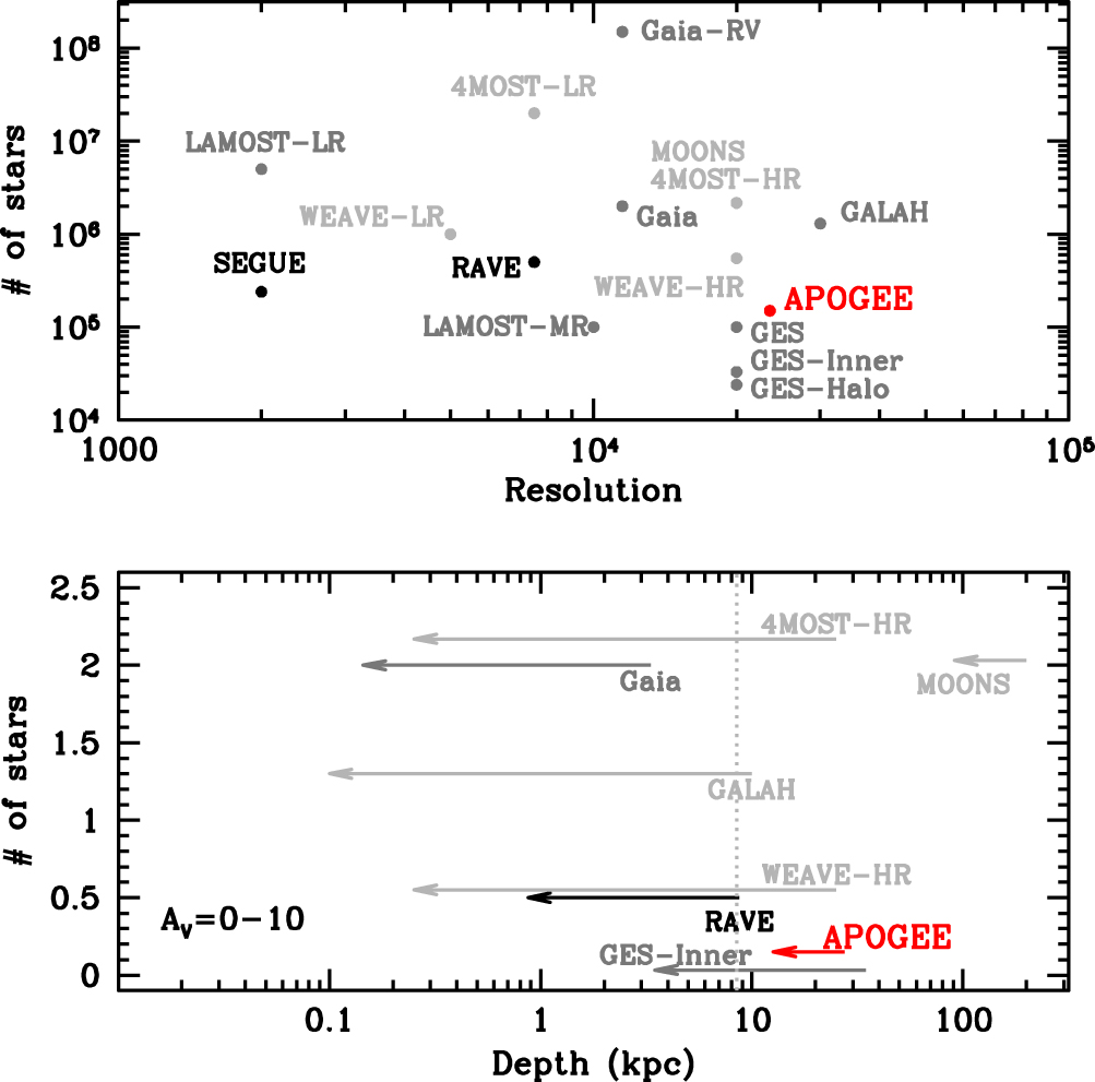
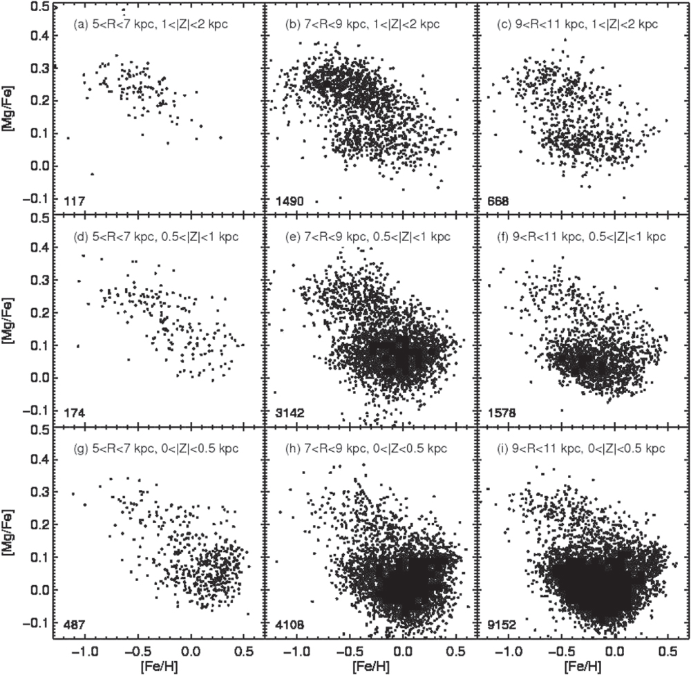
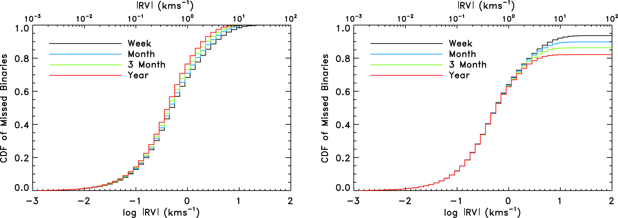