An Accurate Centroiding Algorithm for PSF Reconstruction

A Point Spread Function (PSF) is one of the major systematics in weak lensing measurements. It introduces both multiplicative bias and additive bias. There are numerous methods in the literature devoted to correcting PSF effects (Kaiser et al. 1995; Bertin & Arnouts 1996; Maoli et al. 2000; Rhodes et al. 2000; Bernstein & Jarvis 2002; Bridle et al. 2002; Bacon & Taylor 2003; Hirata & Seljak 2003; Refregier 2003; Heymans et al. 2005; Zhang 2010, 2011; Bernstein & Armstrong 2014; Zhang et al. 2015; Luo et al. 2017). Lensfit (Miller et al. 2007, 2013; Kitching et al. 2008) applies a Bayesian based model-fitting approach. The Bayesian Fourier Domain method (Bernstein & Armstrong 2014) carries out Bayesian analysis in the Fourier domain, using the distribution of unlensed galaxy moments as a prior. Additionally, the Fourier_Quad method developed by Zhang (2010, 2011, 2016) and Zhang et al. (2015) uses image moments in the Fourier Domain.

Many simulations are generated to test the accuracy of various methods, e.g., Shear TEsting Program (Heymans et al. 2006; Massey et al. 2007), Great08 (Bridle et al. 2009), Great 10 (Kitching et al. 2010), GREAT3 (Mandelbaum et al. 2014), or Kaggle—the dark matter mapping competition.⁶ Other independent softwares, such as SHERA (Mandelbaum et al. 2012, hereafter M12), have also been designed for specific surveys. But most of those simulations assume that the PSF is perfectly known, which is not the case in reality. The PSF at a position within a galaxy must be reconstructed using nearby star images.

In the GREAT10 star challenge (Kitching et al. 2013), multiple PSF reconstruction methods have been tested, e.g., PSFEx (Bertin 2011), PCA+Krigging (Li et al. 2013), Gaussianlets (Li et al. 2013), B-slpline (Gentile et al. 2013), Inverse Distance Weighting, Radial Basis Function, and Krigging (Bergé et al. 2012). In particular, Lu et al. (2016) tested various interpolation methods to interpolate the PSF power spectrum for Fourier_Quad shear estimator (Zhang et al. 2015), which achieves a <1% level accuracy in GREAT3 simulations.

As for estimating the centroid of stellar images, a recent work by Vakili & Hogg (2016) claims that simple polynomial fitting works very well and is close to saturating the Cramér-Rao lower bound, while the moment-based method does not deliver reliable centroid estimation. Our method, though, based on fitting the phase slope in Fourier space, provides a better centroid estimation in terms of scatter.

We describe our methodology along with polynomial fitting in Section 2. In Section 3, we describe the simulations to test our method. The results are discussed in Section 4, and we summarize and conclude in Section 5.

In this section, we describe our centroid measurement method along with polynomial fitting method with a Gaussian smooth kernel.

2.1. Fourier Space Phase Fitting (FPF)

Given an image $I({\boldsymbol{x}})$ and its centroid ${{\boldsymbol{x}}}_{{\rm{c}}}$, the Fourier transformation of the image is simply

$$\begin{eqnarray}&&f({\boldsymbol{k}})=\displaystyle \frac{1}{2\pi }\iint I({\boldsymbol{x}}){e}^{-i{\boldsymbol{k}}\cdot {\boldsymbol{x}}}\,d{\boldsymbol{x}},\end{eqnarray} \tag{ 1 }$$

where $f({\boldsymbol{k}})$ can be written as

$$\begin{eqnarray}&&f({\boldsymbol{k}})=| f({\boldsymbol{k}})| \,{e}^{i\angle f({\boldsymbol{k}})},\end{eqnarray} \tag{ 2 }$$

with $\angle (f)$ as the phase. Given that the centroid of a noise-free PSF image $I({\boldsymbol{x}})$ is defined as

$$\begin{eqnarray}&&{{\boldsymbol{x}}}_{{\rm{c}}}:= \displaystyle \frac{\iint {\boldsymbol{x}}\,I({\boldsymbol{x}})d{\boldsymbol{x}}}{\iint I({\boldsymbol{x}})d{\boldsymbol{x}}},\end{eqnarray} \tag{ 3 }$$

we find that the centroid ${{\boldsymbol{x}}}_{{\rm{c}}}$ in real space corresponds to the slope of phase near ${\boldsymbol{k}}=0$, i.e.,

$$\begin{eqnarray}&&{{\boldsymbol{x}}}_{{\rm{c}}}=-{\rm{\nabla }}\angle f(0).\end{eqnarray} \tag{ 4 }$$

The proof is shown in the Appendix A.

In the case that the image is symmetric about the centroid, which is usually the case in the vicinity of the centroid, the image value is real. Then, according to the Fourier transformation properties, we can deduce that

$$\begin{eqnarray}&&f({\boldsymbol{k}})=f(-{\boldsymbol{k}})={f}^{* }({\boldsymbol{k}}).\end{eqnarray} \tag{ 5 }$$

As a result, $f({\boldsymbol{k}})$ is also a real function, meaning the imaginary part vanishes, and the phase function is zero. Any anisotropy can further introduce a nonzero imaginary part, which can be reflected by the phase.

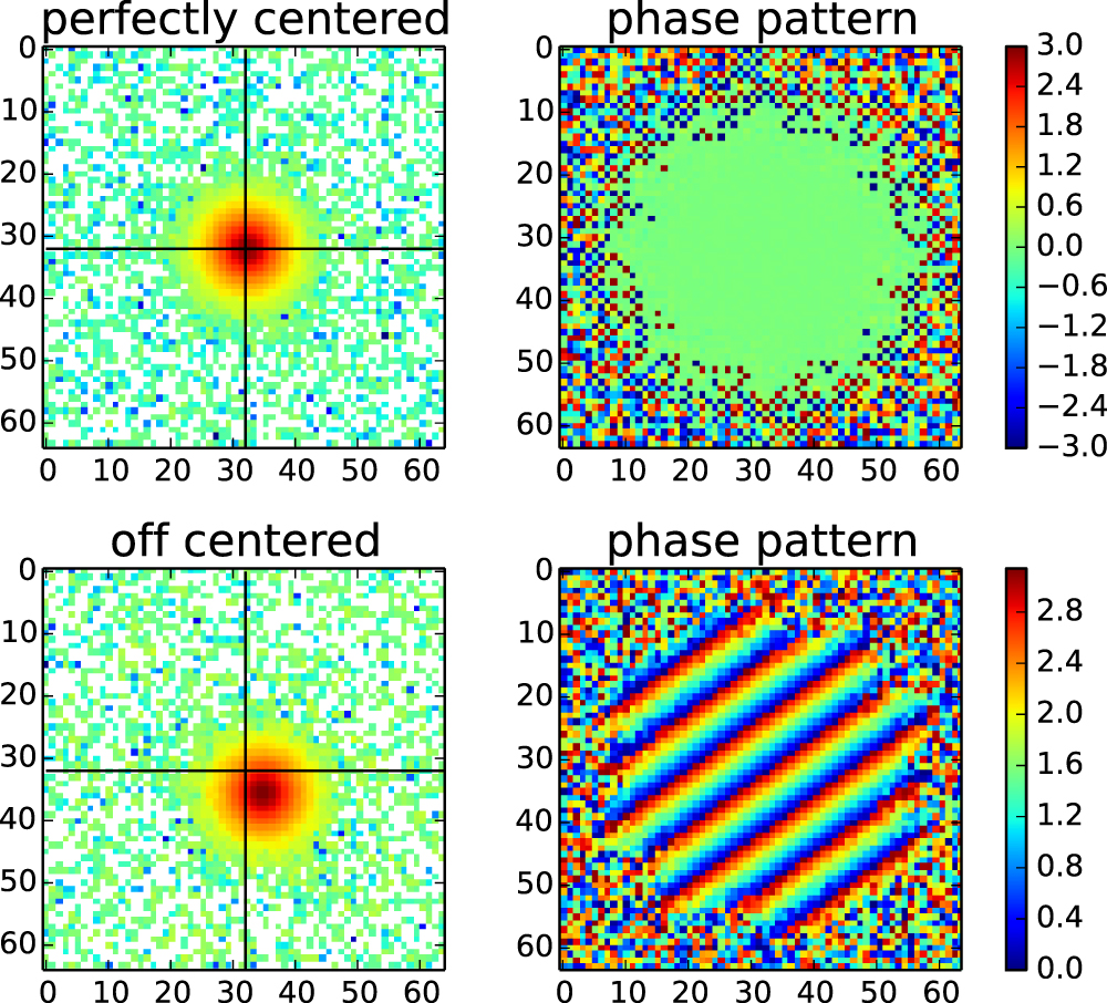
Figure 1 shows an example of how an off-center star image affects the phase pattern in Fourier space. The phase will be zero if the image is perfectly centered, while a stripe pattern will be present if the image is off-center.

Zoom In Zoom Out Reset image size

After discretization, the derivative becomes a minimization problem:

$$\begin{eqnarray}&&{\chi }^{2}=\displaystyle \sum _{{\boldsymbol{k}}}w({\boldsymbol{k}}){[\angle (f({\boldsymbol{k}}){e}^{-i\phi ({\boldsymbol{k}})})]}^{2}\end{eqnarray} \tag{ 6 }$$

where $f({\boldsymbol{k}})={f}_{{\rm{p}}}({\boldsymbol{k}})+{f}_{{\rm{n}}}({\boldsymbol{k}})$ is the Fourier transform of the PSF (${f}_{{\rm{p}}}({\boldsymbol{k}})$) with noise (${f}_{{\rm{n}}}({\boldsymbol{k}})$), and $\phi ({\boldsymbol{k}})$ is the modeled phase pattern of $f({\boldsymbol{k}})$, which depends on the PSF ($f({\boldsymbol{k}})$), the centroid (${{\boldsymbol{x}}}_{{\rm{c}}}$). The observed image is a matrix with real values, so its Fourier transformation satisfies the conditions that are $f(-{\boldsymbol{k}})={f}^{* }({\boldsymbol{k}})$ and $\phi (-{\boldsymbol{k}})=-\phi ({\boldsymbol{k}})$.

For a symmetric PSF, the phase is simply related with the centroids linearly:

$$\begin{eqnarray}&&\phi ={k}_{x}{x}_{{\rm{c}}}+{k}_{y}{y}_{{\rm{c}}}.\end{eqnarray} \tag{ 7 }$$

Nevertheless, the higher-order anisotropy that shifts centroids should be fitted with a higher-order (here we apply third-order) polynomial to capture this effect,

$$\begin{eqnarray}&&\phi ={k}_{x}{x}_{{\rm{c}}}+{k}_{y}{y}_{{\rm{c}}}+{\alpha }_{1}{k}_{x}^{3}+{\alpha }_{2}{k}_{x}^{2}{k}_{y}+{\alpha }_{2}{k}_{x}{k}_{y}^{2}+{\alpha }_{4}{k}_{y}^{3},\end{eqnarray} \tag{ 8 }$$

where {α₁, α₂, α₃, α₄} are free parameters.

In the Appendix B, we show that the weights bearing the analytical form

$$\begin{eqnarray}w({\boldsymbol{k}})=\left\{\begin{array}{ll}\tfrac{2\,| f({\boldsymbol{k}}){| }^{2}}{| {f}_{{\rm{n}}}({\boldsymbol{k}}){| }^{2}}, & | {f}_{{\rm{n}}}({\boldsymbol{k}})| \ll | {f}_{{\rm{p}}}({\boldsymbol{k}})| \\ 0, & | {f}_{{\rm{n}}}({\boldsymbol{k}})| \approx | {f}_{{\rm{p}}}({\boldsymbol{k}})| \end{array}\right.\end{eqnarray} \tag{ 9 }$$

can out-weight the noise while preserve as many data points as possible for the fitting.

2.2. Polynomial Fitting Method

We follow Vakili & Hogg (2016) and apply a fixed Gaussian kernel

$$\begin{eqnarray}&&k(x)=\displaystyle \frac{1}{2\pi {w}^{2}}\exp (-{x}^{2}/2{w}^{2}).\end{eqnarray} \tag{ 10 }$$

where w is 1.2 pixels given that the PSF FWHM is 2.8 pixels, to smooth the image before fitting the centroids with two-dimensional (2D) polynomial

$$\begin{eqnarray}&&P(x,y)=a+{bx}+{cy}+{{dx}}^{2}+{exy}+{{fy}}^{2}.\end{eqnarray} \tag{ 11 }$$

Only the central 3 × 3 patch around the brightest pixels are used to solve the coefficients $X=\{a,b,c,d,e,f\}$. The design matrix A can be constructed as

$$\begin{eqnarray}A=\left(\begin{array}{cccccc}1 & {x}_{1} & {y}_{1} & {x}_{1}^{2} & {x}_{1}{y}_{1} & {y}_{1}^{2}\\ 1 & {x}_{2} & {y}_{2} & {x}_{2}^{2} & {x}_{2}{y}_{2} & {y}_{2}^{2}\\ \vdots & \vdots & \vdots & \vdots & \vdots & \vdots \\ 1 & {x}_{9} & {y}_{9} & {x}_{9}^{2} & {x}_{9}{y}_{9} & {y}_{9}^{2}\end{array}\right).\end{eqnarray} \tag{ 12 }$$

Then the coefficients can be determined by solving

$$\begin{eqnarray}&&X={({A}^{{\rm{T}}}A)}^{-1}{A}^{{\rm{T}}}Z\end{eqnarray} \tag{ 13 }$$

where Z is the pixels of the flattened 3 × 3 patch. The centroids can be then determined by those coefficients

$$\begin{eqnarray}&&\left(\begin{array}{c}{x}_{c}\\ {y}_{c}\end{array}\right)={D}^{-1}\left(\begin{array}{c}-b\\ -c\end{array}\right),\end{eqnarray} \tag{ 14 }$$

where $D=\left(\begin{array}{cc}2d & e\\ e & 2f\end{array}\right),$ is the curvature matrix,

We simulated two sets of images, one uses GalSim (Rowe et al. 2015) and the other is based on Principal Components (PCs) decomposed from CFHT w2 stellar images. The GalSim simulation provides a set of optical effects. The CFHT simulation is used for exploring how much shift is caused by the anisotropy in real surveys.

3.1. GalSim Stellar Image

We use GalSim to simulate three sets of star images with different signal-to-noise ratios: S/N ∼ 50, S/N ∼ 100, and S/N ∼ 200. The S/N is not strictly 50, 100, or 200 due to the fact that we simulate the images using Exposure Time Calculator from a uniform magnitude distribution centered at each S/N.

We apply a Moffat profile for all of the stellar images and a uniform distribution for the r_d and β in

$$\begin{eqnarray}&&I(r)={\left(1+\displaystyle \frac{{r}^{2}}{{r}_{{\rm{d}}}^{2}}\right)}^{-\beta },\end{eqnarray} \tag{ 15 }$$

where I(r) is the 2D brightness distribution. After we generate the stellar images, we shift the centers using two uniform distributions from −0.5 to 0.5 to each image as input centroid value. Then, we convolve the images with optical anisotropy effect coma as shown in Figure 2. We exaggerate this effect for better illustration; in fact, it is hard to notice by visual inspection. Finally, we add Gaussian noise using GalSim to simulate different S/Ns in stellar images. Noise and randomly oriented optical anisotropy contribute additional dispersion to the centroid of the image.

Zoom In Zoom Out Reset image size

3.2. CFHT w2 Stellar Image

In real observations, atmospheric seeing dilutes the observed objects and introduces extra ellipticity and shift of the centroid. The background sky also shifts the centroid randomly. For high S/N images, the centroid-shifting mechanism is dominated by atmospheric seeing. An accurate centroid estimation method should be designed to capture this shifting and correct for it.

In this simulation, we focus on testing this high-order centroid-shifting effect based on real data from CFHTLens survey field w2, which contains seven exposures, with 10-minute exposure for each.

The procedure of this simulation is described as follows:

• 1.  
  Select all of the stellar images with S/N > 100 and without saturation from CFHT w2 area (there are ∼600,000 stars in total).
• 2.  
  Extract components using PCA without centroiding.
• 3.  
  Generate 10000 stellar images using the first 16 PCs. The coefficients of the PCs are randomly drawn from the parent distribution of the original images.
• 4.  
  Calculate the centroid using brightness weighted moments using

  $$\begin{eqnarray}&&{{\boldsymbol{x}}}_{0}=\displaystyle \frac{\iint {\boldsymbol{x}}\,I({\boldsymbol{x}})d{\boldsymbol{x}}}{\iint I({\boldsymbol{x}})d{\boldsymbol{x}}}.\end{eqnarray} \tag{ 16 }$$

  to be the reference. This can be considered as the real input center when there is no noise.

The first six PCs decomposed from CFHT w2 stellar images are shown in Figure 3. We preserve the dipoles by not centroiding the postage stamp images so that the asymmetry can be directly reconstructed by the dipoles.

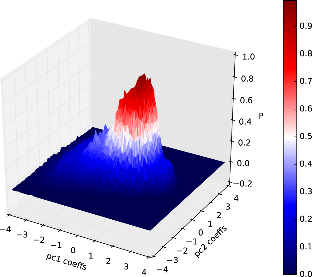
Zoom In Zoom Out Reset image size

Note that although we use PCA to decompose PSF images, their PCs do not follow Gaussian distributions, as is shown in Figure 4. Thus, it is necessary to generate CFHT-like images according to the original distribution function of PCs. We sample this distribution by picking random data points of PCs derived from original images.

Zoom In Zoom Out Reset image size

We display the images from two simulations in Figure 5. The right panel shows the PSF from GalSim simulation and the left panel shows the CFHT-like simulation. Despite the anisotropy effect added to the GalSim PSFs, we still cannot observe its existence by visual inspection.

Zoom In Zoom Out Reset image size

We demonstrate the performance of three centroiding methods Figure 6, i.e., polynomial fitting, first-order phase fitting and third-order phase fitting based on two simulations, GalSim and CFHT-like simulations. In the GalSim simulation, we arbitrarily enlarge the effect of anisotropy by adjusting the comma size and orientation to test the performance of each method. For the CFHT simulations, which are based on the images from CFHT, the anisotropy is marginally affected by the coma. The major systematic that introduces anisotropy is mostly from atmospheric seeing.

Zoom In Zoom Out Reset image size

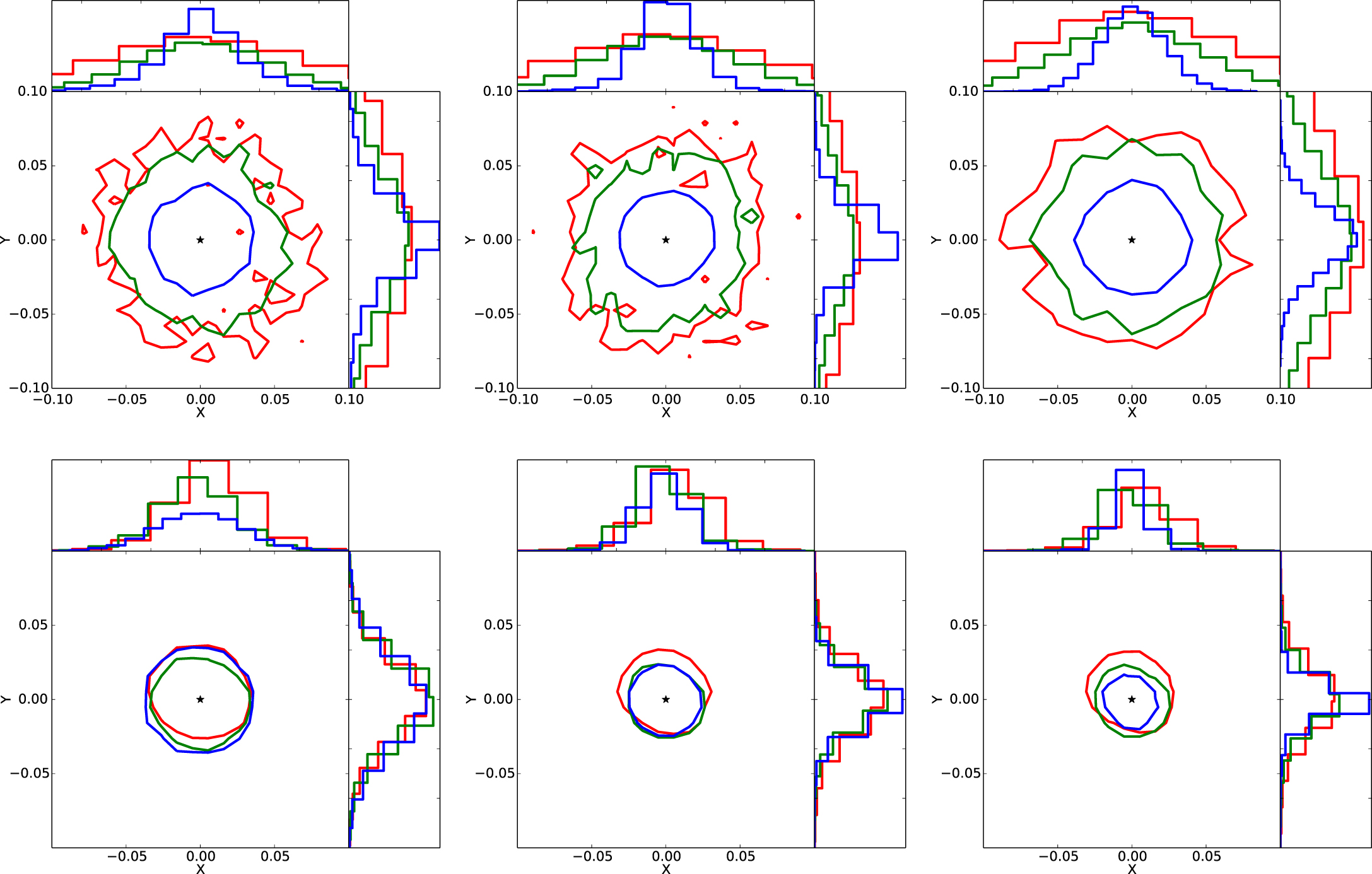
The top three panels show the results from GalSim simulation, and the bottom three are from the CFHT-like simulation. From left to right, the S/N = 50, 100, 200, respectively. In general, the first-order FPF is already better than polynomial fitting in both simulations, and the third-order FPF significantly improves the centroid estimation. In the CFHT-like S/N = 50 simulation, all three methods perform similarly due to the fact that the sky background noise dominates the scatter budget. The quantitative comparison is listed in Table 1.

In the GalSim simulation, where the optical anisotropy dominates the scatter budget, the scatter from the third-order FPF is ∼3 times smaller than that from polynomial fitting in all S/N branches.

In the CFHT-like simulation, the performance of the three methods is similar in the S/N = 50 branch. For the S/N =100 branch, which is often used in real analysis, the scatter from the third-order FPF is ∼1.5 smaller than that from polynomial fitting. This difference expands to ∼2.0 for the S/N = 200 branch. As the effect of noise drops, the third-order FPF displays better and better performances relative to polynomial fitting, due to its ability to accurately capture higher-order anisotropy features.

This is further illustrated by the GalSim simulation, where higher-order anisotropy dominates the scatter budget. In all S/N branches, the scatter from the third-order FPF is ∼3 times smaller than that from polynomial fitting.

Centroiding is the first and most important procedure for PSF reconstruction. An accurate PSF reconstruction further affects shear measurement. We develop our centroid estimation method in Fourier space—a third-order FPF.

In the GalSim simulation, the centroiding shift is dominated by optical anisotropy. The scatter of the third-order FPF is smaller than that of the polynomial fitting method by a factor of ∼2–3, from the S/N = 50 to S/N = 200 branch.

In the CFHT-like simulation, where the higher-order anisotropy is much smaller than GalSim simulation, we found that for the S/N = 50 images, background noise dominates the scatter, while for the S/N = 200, optical anisotropy plays a major role for this scatter. Therefore, the third-order FPF performs similarly in the S/N = 50 branch, but with half the scatter of the polynomial fitting method in the S/N = 200 branch.

Therefore, we conclude that the third-order FPF method so far provides the most accurate estimation in finding centroids among the methods in this study. Additionally, the processing speed of the third-order FPF is about 100 ms per image applying the conjugate gradient method, which is comparable to the polynomial fitting (50 ms) on a python platform.

The scatter caused by noise cannot well corrected for any methods, but for scatter introduced by optical anisotropies, the third-order FPF can capture the shift precisely. For the polynomial method, the scatter is about 0.08, leading to a 0.4% increase in PSF size, and this reduces to about 0.2% for the third-order FPF. This scatter will effect the shape measurement in two folds. First, the shape estimator based on the image moments method applies a size cut so that galaxies with $R=1-\tfrac{{T}_{\mathrm{psf}}}{{T}_{\mathrm{gal}}\times O(m)}\leqslant \tfrac{1}{3}$ are discarded, and more galaxies are hence excluded by a larger PSF size. Second, a larger PSF size leads to over-correction of the smearing effect and further biases the shape estimation. This is a generic case not only in the CFHT survey but also in the LSST. For a space telescope, where noise is sub-dominant, the scatter mechanism third-order FPF should be a better choice for PSF centroiding.

This work was supported by the following programs: NSFC (Nos. 11503064), Shanghai Natural Science Foundation, grant No. 15ZR1446700. J.Z. is supported by the NSFC grants (11673016, 11433001, 11621303) and the National Key Basic Research Program of China (2015CB857001). L.P.F. acknowledges the support from NSFC grants 11673018, 11722326 & 11333001, STCSM grant 16ZR1424800 & 188014066, and SHNU grant DYL201603. G.L. is supported by NSFC (No.11673065, 11273061 and 1133008) and the 973 program (No. 2015CB857003). Z.H.F. acknowledges support from NSFC grants of 11333001, 11173001, and 11653001.

This work was also supported by the High Performance Computing Resource in the Core Facility for Advanced Research Computing at Shanghai Astronomical Observatory.

First, we calculate the derivative of $f({\boldsymbol{k}})$ with respect to k_x at ${\boldsymbol{k}}=0$:

$$\begin{eqnarray}{\left.\displaystyle \frac{\partial }{\partial {k}_{x}}\right|}_{{\boldsymbol{k}}=0}f({\boldsymbol{k}}) & = & {\left.\displaystyle \frac{\partial }{\partial {k}_{x}}\right|}_{{\boldsymbol{k}}=0}\left\{\displaystyle \frac{1}{2\pi }\iint I({\boldsymbol{x}}){e}^{-i{\boldsymbol{k}}\cdot {\boldsymbol{x}}}\,d{\boldsymbol{x}}\right\}\\ & = & {\left.\displaystyle \frac{\partial }{\partial {k}_{x}}\right|}_{{k}_{x}=0}\left\{\displaystyle \frac{1}{2\pi }\iint I(x,y){e}^{-{{ik}}_{x}x}\,{dxdy}\right\}\\ & = & \displaystyle \frac{1}{2\pi }\iint I(x,y){\left.\displaystyle \frac{\partial }{\partial {k}_{x}}\right|}_{{k}_{x}=0}{e}^{-{{ik}}_{x}x}\,{dxdy}\\ & = & -\displaystyle \frac{i}{2\pi }\iint I(x,y)x\,{dxdy}\\ & = & -{{ix}}_{{\rm{c}}}\,\displaystyle \frac{1}{2\pi }\iint I(x,y){dxdy},\\ & = & -{if}(0){x}_{{\rm{c}}}.\end{eqnarray} \tag{ 17 }$$

Next, we relate the derivative of $f({\boldsymbol{k}})$ with respect to k_x with that of $\angle f({\boldsymbol{k}})$:

$$\begin{eqnarray}{\left.\displaystyle \frac{\partial }{\partial {k}_{x}}\right|}_{{\boldsymbol{k}}=0}f({\boldsymbol{k}}) & = & {\left.\displaystyle \frac{\partial }{\partial {k}_{x}}\right|}_{{\boldsymbol{k}}=0}\{| f({\boldsymbol{k}})| \,{e}^{i\angle f({\boldsymbol{k}})}\}\\ & = & | f(0)| \,{e}^{i\angle f(0)}\left(i{\left.\displaystyle \frac{\partial }{\partial {k}_{x}}\right|}_{{\boldsymbol{k}}=0}\angle f({\boldsymbol{k}})\right)\\ & & +\displaystyle \frac{\partial f(0)}{\partial {k}_{x}}\,{e}^{i\angle f(0)}\\ & = & {if}(0){\left.\displaystyle \frac{\partial }{\partial {k}_{x}}\right|}_{{\boldsymbol{k}}=0}\angle f({\boldsymbol{k}}).\end{eqnarray} \tag{ 18 }$$

Comparing Equation (17) and Equation (18), we find

$$\begin{eqnarray}&&{x}_{{\rm{c}}}=-{\left.\displaystyle \frac{\partial }{\partial {k}_{x}}\right|}_{{\boldsymbol{k}}=0}\angle f({\boldsymbol{k}}),\end{eqnarray} \tag{ 19 }$$

and similarly,

$$\begin{eqnarray}&&{y}_{{\rm{c}}}=-{\left.\displaystyle \frac{\partial }{\partial {k}_{y}}\right|}_{{\boldsymbol{k}}=0}\angle f({\boldsymbol{k}}).\end{eqnarray} \tag{ 20 }$$

Thus, we obtain

$$\begin{eqnarray}&&{{\boldsymbol{x}}}_{{\rm{c}}}=-{\rm{\nabla }}\angle f(0).\end{eqnarray} \tag{ 21 }$$

Suppose that the Fourier transform of the noise-free PSF is ${f}_{{\rm{p}}}({\boldsymbol{k}})$, and the noise has magnitude $| {f}_{{\rm{n}}}({\boldsymbol{k}})|$ and a random phase. Given $f={f}_{{\rm{p}}}+{f}_{{\rm{n}}}$, we can deduce the scatter of $\angle f$ in terms of its variance.

When $| {f}_{{\rm{n}}}| \ll | {f}_{{\rm{p}}}|$ (without loss of generality, we let ${f}_{{\rm{p}}}\in {\mathbb{R}}$),

$$\begin{eqnarray}\mathrm{Var}(\angle f) & = & \langle {(\angle f-\langle \angle f\rangle )}^{2}\rangle \\ & = & \langle {(\angle ({f}_{{\rm{p}}}+{f}_{{\rm{n}}})-\angle {f}_{{\rm{p}}})}^{2}\rangle \\ & = & \langle {(\mathrm{Im}({f}_{{\rm{n}}}){{{\rm{\nabla }}}_{\mathrm{Im}}\angle f| }_{f={f}_{{\rm{p}}}})}^{2}\rangle \\ & = & \displaystyle \frac{1}{2}| {f}_{{\rm{n}}}{| }^{2}{\left({\left.\displaystyle \frac{{{df}}^{-1}}{{df}}\right|}_{f={f}_{{\rm{p}}}}\right)}^{2}\\ & = & \displaystyle \frac{| {f}_{{\rm{n}}}{| }^{2}}{2\,| {f}_{{\rm{p}}}{| }^{2}},\end{eqnarray} \tag{ 22 }$$

where ∇_Im denotes the directional derivative along the imaginary part.

The weights should be inversely proportional to the variances. We take

$$\begin{eqnarray}&&w({\boldsymbol{k}})=\mathrm{Var}{(\angle f)}^{-1}=\displaystyle \frac{2\,| {f}_{{\rm{p}}}{| }^{2}}{| {f}_{{\rm{n}}}{| }^{2}}\approx \displaystyle \frac{2\,| f{| }^{2}}{| {f}_{{\rm{n}}}{| }^{2}}.\end{eqnarray} \tag{ 23 }$$

When $| {f}_{{\rm{n}}}| \approx | {f}_{{\rm{p}}}|$, the scatters of $\angle f$ are so large that such pixels do not provide useful information of $\angle {f}_{{\rm{p}}}$. Thus, we take

$$\begin{eqnarray}&&w({\boldsymbol{k}})=0.\end{eqnarray} \tag{ 24 }$$