


Abstract
We report the discovery of a transiting planet first identified as a candidate in Sector 1 of the Transiting Exoplanet Survey Satellite (TESS), and then confirmed with precision radial velocities. HD 1397b has a mass of  , a radius of
  , and orbits its bright host star (V = 7.8 mag) with an orbital period of
  d on a moderately eccentric orbit (
 ). With a mass of
  , a radius of
  , and an age of
  Gyr, the solar-metallicity host star has already departed from the main sequence. We find evidence in the radial velocity measurements of a secondary signal with a longer period. We attribute it to the rotational modulation of stellar activity, but a long-term radial velocity monitoring would be necessary to discard if this signal is produced by a second planet in the system. The HD 1397 system is among the brightest ones currently known to host a transiting planet, which will make it possible to perform detailed follow-up observations in order to characterize the properties of giant planets orbiting evolved stars.
Export citation and abstract BibTeX RIS
1. Introduction
Throughout the past two decades, several ground-based, small-aperture, wide-field photometric surveys (e.g., Bakos et al. 2004; Pollacco et al. 2006; Pepper et al. 2007; Bakos et al. 2013; Talens et al. 2017) have efficiently detected and characterized the population of short-period transiting giant planets orbiting bright stars across the whole sky. These discoveries have triggered significant advances in the study of the formation and evolution of planetary systems, and have been targets of detailed follow-up observations to study their orbital configurations (e.g., Triaud et al. 2010; Zhou et al. 2015; Esposito et al. 2017) and atmospheric compositions (e.g., Chen et al. 2018; Jensen et al. 2018; Spake et al. 2018). Nonetheless, due to strong observational biases produced by the Earth's atmosphere and the limited duty cycle of ground-based facilities, there is still a region of parameter space of giant planets that is vastly unexplored. Specifically, transiting systems of giant planets having orbital periods longer than ≈10 days have scarcely been detected from the ground (Kovács et al. 2010; Lendl et al. 2014; Brahm et al. 2016; Hellier et al. 2017). Additionally, due to the decrease in transit depth, we only have a handful of giant planets orbiting stars that have recently left the main sequence with radii larger than  (Hartman et al. 2012; Smith et al. 2013; Rabus et al. 2016; Bento et al. 2018). The characterization of transiting giant planets having periods longer than 10 days and/or orbiting evolved stars, is important for understanding the processes that govern the formation, evolution, and fate of giant planets. The detailed study of the distribution of eccentricities and spin–orbit angles of giant planets orbiting beyond 0.1 au can be used to constrain migration theories (Dong et al. 2014; Petrovich & Tremaine 2016; Anderson & Lai 2017), while the characterization of planets orbiting giant and subgiant stars can be used to infer the nature of the inflation mechanism of hot Jupiters (Lopez & Fortney 2016), characterizing tidal interactions (e.g., Villaver & Livio 2009), and understanding the Lithium excess observed in some evolved stars (e.g., Aguilera-Gómez et al. 2016). Very recently, the K2 mission (Howell et al. 2014) started to contribute to the detection of giant planets orbiting bright stars having P > 10 days (e.g., Shporer et al. 2017; Brahm et al. 2018; Jordán et al. 2019; Yu et al. 2018), and giant planets orbiting evolved stars (e.g., Grunblatt et al. 2017; Jones et al. 2018). While not being its primary scientific driver, the Transiting Exoplanet Survey Satellite (TESS) mission (Ricker et al. 2015) is expected to discover several hundred giant planets orbiting bright stars (V < 12 mag) having periods longer than 10 days and/or orbiting evolved stars (Barclay et al. 2018). Therefore, it is expected that TESS will yield for the first time a statistically significant sample for these kind of objects that will be useful for constraining theories of planetary formation and evolution. Interestingly, an important fraction of the first confirmed giant planets from TESS orbit evolved stars (Wang et al. 2019; Huber et al. 2019; Rodriguez et al. 2019).
In this study we present the discovery of HD 1397b, the first giant planet discovered by the TESS mission with an orbital period longer than 10 days. In addition to its long period, the host star is a bright (V = 7.8) subgiant star, making this a very interesting system for further study.
2. Observations
2.1. Transiting Exoplanet Survey Satellite
Between 2018 July 25 and 2018 August 22, the TESS mission observed HD 1397 (TIC 394137592, TOI00120.01) with its Camera 3 during the monitoring of the first TESS sector. Observations were performed with a cadence of 2 minutes. Photometric data of HD 1397 were analyzed with the Science Processing Operations Center (SPOC) pipeline, which is a modified version of the pipeline used for the NASA Kepler mission (J. Jenkins et al. 2019, in preparation). This light curve was released to the community on 2018 September 15 as an alert. The alert did not report warning flags that could be associated with false positive scenarios. In particular, there is no statistical difference between transit depths, and there are no significant centroid offsets of the point-spread function (PSF) during the transits.
The TESS light curve of HD 1397 is presented in Figure 1, after removing flagged data point reaction wheel desaturation events, and shows the presence of two clear, moderately deep (≈2500 ppm) transits separated by ≈11.5 days.
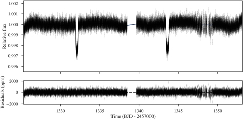
Figure 1. TESS two-minute cadence light curve from Sector 1 for HD 1397. The gray points correspond to the TESS flux measurements while the solid line corresponds to the model having the parameters described in Section 3.3. The bottom panel shows the corresponding residuals.
Download figure:
Standard image High-resolution imageHD 1397 was also observed during the monitoring of the second TESS sector. However, no two-minute cadence light curve was processed by the SPOC pipeline. The reason for this could be related to the position of the star in the TESS detector, because it was located just a few pixels from the edge. Nonetheless, we extracted a light curve from the full-frame images (FFIs) using tesseract10 (F. Rojas et al. 2019 in preparation). This light curve, presented in Table 1, has a cadence of 30 minutes and shows three additional transits with the same depth and periodicity to those observed in Sector 1 (see Figure 2). No additional features that could be associated to other planets in the system can be identified. We use this light curve along with the one of Sector 1 obtained with a cadence of 2 minutes for performing the global analysis described in Section 3.3.
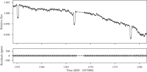
Figure 2. Same as in Figure 1, but for the TESS data of Sector 2 obtained in long (30 minutes) cadence.
Download figure:
Standard image High-resolution imageTable 1. Thirty-minute Cadence TESS Light Curve Data for HD 1397 Obtained from the tesseract Extraction of the FFIs of Sector 2
| BJD | Flux | σFlux | Instrument |
|---|---|---|---|
| 2458354.138977051 | 1.00148 | 0.00006 | TESS |
| 2458354.159851074 | 1.00129 | 0.00006 | TESS |
| 2458354.180664063 | 1.00126 | 0.00006 | TESS |
| 2458354.201477051 | 1.00136 | 0.00006 | TESS |
| 2458354.222351074 | 1.00131 | 0.00006 | TESS |
| 2458354.243164063 | 1.00142 | 0.00006 | TESS |
| 2458354.263977051 | 1.00116 | 0.00006 | TESS |
| 2458354.284851074 | 1.00114 | 0.00006 | TESS |
| 2458354.305664063 | 1.00129 | 0.00006 | TESS |
| 2458354.326477051 | 1.00125 | 0.00006 | TESS |
| 2458354.347351074 | 1.00107 | 0.00006 | TESS |
Only a portion of this table is shown here to demonstrate its form and content. A machine-readable version of the full table is available.
Download table as: DataTypeset image
2.2. High-resolution Spectroscopy
We started the radial velocity follow-up of HD 1397 a couple of hours after the first alerts of TESS Sector 1 were made public. We obtained two spectra with the High Accuracy Radial Velocity Planet Searcher (HARPS) spectrograph (Mayor et al. 2003) installed at the ESO 3.6 m telescope at La Silla Observatory on two consecutive nights. We adopted an exposure time of 300 s and pointed the comparison fiber to the background sky. Additionally, we obtained 35 spectra with the The Fiber Dual Echelle Optical Spectrograph (FIDEOS; Vanzi et al. 2018) installed at the 1 m telescope on the same observatory. FIDEOS observations were obtained on six consecutive nights. For these observations we adopted an exposure time of 600 s and the comparison fiber was used to trace the instrumental radial velocity drift by observing a ThAr lamp. The HARPS and FIDEOS data were processed with the CERES package (Brahm et al. 2017a), which automatically performs optimal spectral extraction from the raw images, wavelength calibration, instrumental drift correction, and the computation of the radial velocities and bisector spans. The radial velocities were computed with the cross-correlation technique using a binary mask with a set of lines compatible with a G2-type star. These radial velocities were consistent with an absence of large variations that could have been produced by a stellar companion, and they hinted the presence of a relatively low-amplitude signal (≈30 m s−1) in phase with the photometric ephemeris. Additionally, no secondary peaks were identified in the cross-correlation function that could have indicated the presence of possible background diluted eclipsing binaries.
We then proceeded to perform an intensive radial velocity monitoring of HD 1397 with the Fiber-fed Extended Range Optical Spectrograph (FEROS) installed at the MPG 2.2 m telescope at La Silla Observatory (Kaufer et al. 1999). Three additional HARPS spectra were acquired during this period. FEROS observations were performed with the simultaneous calibration mode and the adopted exposure time was of 300 s. We obtained 88 spectra on a time span of 80 nights. FEROS data were also processed with the CERES package. In addition to the bisector span measurements, the S-index activity indicator was computed for each spectrum as described in Jenkins et al. (2008) and Jones et al. (2017). HD 1397 presents significant and time-variable chromospheric emission as gauged from the Ca ii H & K lines of the FEROS and HARPS spectra. The radial velocities, bisector spans, and S-indexes obtained with the three instruments are presented in the
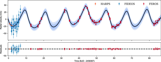
Figure 3. Top panel presents the radial velocity curve for HD 1397 obtained with HARPS (orange), FIDEOS (blue), and FEROS (red). The black line corresponds to the Keplerian model plus Gaussian process with the posterior parameters found in Section 3.3. The bottom panel shows the residuals.
Download figure:
Standard image High-resolution image
Figure 4. Top panel: radial-velocity–bisector-span scatter plot for the FEROS observations of HD 1397. No correlation is observed. Bottom panel: radial-velocity–S-index scatter plot for the FEROS observations. A marginally significant correlation at the 95% level of confidence is observed.
Download figure:
Standard image High-resolution image3. Analysis
3.1. Properties of the Host Star
We analyzed the co-added FEROS spectra to obtain the atmospheric parameters of HD 1397. We used the ZASPE code (Brahm et al. 2017b), which compares the observed spectrum to a grid of synthetic models generated from the ATLAS9 model atmospheres (Castelli & Kurucz 2003). The search for the optimal model is performed only in the spectral zones that are most sensitive to changes in the atmospheric parameters. The errors in the derived parameters are obtained from Monte Carlo simulations where the depth of the spectral lines of the synthetic models are perturbed in order to properly account for the systematic model mismatch as the main source of the error budget. We obtained that HD 1397 has an effective temperature of  , a surface gravity of
  , a metallicity of
 ![$[\mathrm{Fe}/{\rm{H}}]\,=+0.04\pm 0.05\,\mathrm{dex}$](https://content.cld.iop.org/journals/1538-3881/158/1/45/revision1/ajab279aieqn11.gif) , and a projected rotational velocity of
, and a projected rotational velocity of  .
.
We followed two similar procedures for estimating the physical parameters of the host star. The first procedure consists of two steps and was presented in Brahm et al. (2018). The first step is to compute the stellar radius from the publicly available broadband photometry and the parallax delivered by GAIA DR2. Briefly, we interpolate the stellar models presented in Baraffe et al. (2015) to generate a synthetic spectral energy distribution (SED) consistent with the atmospheric parameters found for HD 1397. We then generated synthetic magnitudes from the SED by integrating it in different spectral zones, weighted by the corresponding transmission functions of the passband filters presented in Table 2. These synthetic magnitudes were used to estimate the stellar radius ( ) and the extinction factor (AV) by comparing them to the publicly reported magnitudes after converting them to absolute magnitudes using the distance obtained from the GAIA DR2 parallax measurement (Gaia Collaboration et al. 2016, 2018). We obtained the posterior distribution for
  and AV using the emcee Python package (Foreman-Mackey et al. 2013). In order to consider the uncertainty in the atmospheric parameters, we repeated this process for different values of
  sampled from a Gaussian distribution with the parameters obtained with the ZASPE analysis. We find that HD 1397 has a radius of
  and an extinction factor consistent with AV = 0.
Table 2. Stellar Properties of HD 1397
| Parameter | Value | Reference |
|---|---|---|
| Names | HD 1397 | |
| TIC 394137592 | TESS | |
| HIP 1419 | HIPPARCOS | |
| 2MASS J00174714–6621323 | 2MASS | |
| TYC 8846-638-1 | TYCHO | |
| R.A. (J2000) | 00h17m47 14 14 |
TESS |
| Decl. (J2000) | −66d21m3235 |
TESS |
| pmR.A.(mas yr−1) | 64.76 ± 0.05 | GAIA |
| pmDecl. (mas yr−1) | −5.06 ± 0.04 | GAIA |
| π (mas) | 12.54 ± 0.03 | GAIA |
| T (mag) | 7.14 ± 0.03 | TESS |
| B (mag) | 8.47 ± 0.05 | APASS |
| V (mag) | 7.79 ± 0.03 | APASS |
| J (mag) | 6.44 ± 0.02 | 2MASS |
| H (mag) | 6.09 ± 0.05 | 2MASS |
| Ks (mag) | 5.99 ± 0.02 | 2MASS |
| WISE1 (mag) | 6.02 ± 0.09 | WISE |
| WISE2 (mag) | 5.90 ± 0.04 | WISE |
| WISE3 (mag) | 5.99 ± 0.02 | WISE |
 (K) (K) |

|
zaspe |
 (dex) (dex) |

|
zaspe |
![$[\mathrm{Fe}/{\rm{H}}]$](https://content.cld.iop.org/journals/1538-3881/158/1/45/revision1/ajab279aieqn21.gif) (dex) (dex) |

|
zaspe |
 (km s−1) (km s−1) |

|
zaspe |
 ( ( ) ) |

|
PARSEC + GAIA |
 ( ( ) ) |

|
PARSEC + GAIA |
| L⋆ (L⊙) | 4.32 ± 0.19 | PARSEC + GAIA |
| MV (mag) | 3.30 ± 0.06 | PARSEC + GAIA |
| Age (Gyr) |

|
PARSEC + GAIA |
| ρ⋆(g cm−3) |

|
PARSEC + GAIA |
| ρ⋆(g cm−3) | 0.112 ± 0.015 | juliet |
Download table as: ASCIITypeset image
The second step of the first procedure consists in estimating the mass and evolutionary stage of HD 1397 by comparing its effective temperature and radius to those predicted by stellar evolutionary models. Specifically, we use the Yonsei-Yale evolutionary models (Yi et al. 2001), which are interpolated to the metallicity derived for HD 1397. We use the emcee package to compute the posterior distributions for the stellar mass and age. With this procedure we find that HD 1397 has a mass of  and an age of 4.7 ± 0.2 Gyr.
The second procedure that we followed for estimating the stellar physical parameters consists of using the PARSEC isochrones (Bressan et al. 2012), which directly deliver the absolute magnitudes in different bandpasses for a given set of stellar properties. This allow us to skip the SED modeling presented in the previous procedure. We downloaded a grid of PARSEC version 1.1 models11
containing the GAIA (G, GBP, GRP) and 2MASS magnitudes. We then used the spectroscopic temperature, the observed magnitudes and the gaia parallax to estimate the stellar mass and the age of the system via a Markov chain Monte Carlo (MCMC). With this procedure we estimated a stellar mass of  , a stellar radius of
  , and an age of 4.51 ±0.20 Gyr, which are not significantly different to those obtained with SED modeling plus YY isochrones. Due to the greater self-consistency of this second procedure, and because the density obtained with it is closer to the one obtained from the global modeling, we adopted these last set of physical parameters as the final stellar parameters. We have proven that our methodology for estimating the stellar physical parameters produces stellar density values consistent to those obtained via asteroseismic analysis (see Sanford et al. 2019, in preparation). We do not see systematic biases or trends in this comparison, but we observe that the scatter of the residuals is 40% larger than the typical internal error bars. We expect that most of this underestimated error budget originates from the determination of the stellar mass rather than from the stellar radius, because this latter parameter is tightly constrained by the GAIA parallax. For this reason the reported uncertainties for the stellar mass and radius include this 40% inflation of the error bars.
The stellar parameters obtained for HD 1397 are presented in Table 2 along with its observed properties.
3.2. Radial Velocities
Motivated by the slight correlation between the radial velocities and the activity indicators, and the presence of time-correlated residuals in some preliminary modeling of the radial velocities, we proceeded to analyze all the available time series. We computed the generalized Lomb–Scargle periodograms (GLS; Zechmeister & Kürster 2009) for the nondetrended TESS photometry, radial velocities, bisector span measurements, and S-index values. For the TESS photometry we only used the two-minute cadence light curve and we masked out the two transits. The significance of the peaks in the periodograms was evaluated by performing a bootstrap of each time series. The four periodograms are plotted in Figure 5. The bottom panel of Figure 5 shows that the radial velocity measurements are able by themselves to recover with high significance the 11.5-day periodic signal of the planet candidate observed in the TESS transits. Additionally, there are no peaks in the periodograms of the bisector spans and S-index associated to that particular period. Interestingly, the periodogram of the TESS photometry presents a peak close to the orbital period of the system. If the associated signal is not an artifact of the SPOC pipeline, given the large ratio between the radii of the star and the planet, the source of this periodic variation could be associated to changes on the star (e.g., ellipsoidal variations; Welsh et al. 2010) rather than phase curve variations.

Figure 5. GLS power spectra for the TESS photometry, S-index, bisector spans, radial velocities of HD 1397, and window function (black lines from top to bottom). The gray lines represent the 1% significance limits based on bootstrap simulations. The radial velocities present a primary peak at ≈11.5 days (vertical blue line), which is consistent with the orbital period of the planetary candidate obtained from the TESS photometry. The activity indicators present some wide significant peaks that could be responsible for the extra variation observed in the radial velocities.
Download figure:
Standard image High-resolution imageThe periodograms for the radial velocities, bisector span measurements, and the S-index present some wide peaks at longer periods (20–50 days), but they are unresolved due to the short baseline of the observations. The presence of these peaks indicates that the additional radial velocity variation can be produced by rotational modulation of the stellar activity. However, a more extended radial velocity campaign will be needed to confirm this relation.
3.3. Global Modeling
The global modeling of the transit and radial velocities was performed with juliet (Espinoza et al. 2018). The algorithm is similar to exonailer (Espinoza et al. 2016) with the main difference that instead of emcee (Foreman-Mackey et al. 2013), the new algorithm uses MultiNest (Feroz et al. 2009) via the PyMultiNest package (Buchner et al. 2014) in order to both perform posterior sampling and model comparison directly using model evidences. The transits are modeled using batman (Kreidberg 2015) and the radial velocities modeled using radvel (Fulton et al. 2018), where we consider an individual jitter term for each instrument. For limb darkening, we use a quadratic law with the uninformative sampling scheme of Kipping (2013). This enhanced algorithm in turn also has the possibility to include dilution factors and variable mean fluxes for different photometric instruments, as well as the possibility of fitting multiplanetary systems for both transits and radial velocities simultaneously. Variations produced by nonplanetary factors in both the radial velocities and the photometry (e.g., instrumental systematics or nondeterministic astrophysical phenomena) can be modeled within juliet via Gaussian processes (GPs) via both george (Ambikasaran et al. 2015) and celerite (Foreman-Mackey et al. 2017) using any set of external variables. In addition, several types of trends as a function of time can also be modeled in the radial velocities including linear and quadratic trends.
We observe evident smooth long-term trends in both TESS light curves. We model those photometric variations using a distinct GP for each data set. In both cases an exponential kernel was used. For the radial velocity modeling, our initial fits, which considered just the presence of the transiting planet, showed the existence of a time-correlated scatter in the residuals (in line with the peaks beyond 20 days present in Figure 5). We thus performed several fits in order to account for this extra signal and to robustly investigate its nature. We considered models in which this extra periodic signal could be a second planet in the system (via an extra keplerian signal) and where this could come from stellar activity in the form of a quasi-periodic GP; for this latter case, we use the quasi-periodic kernel introduced in Foreman-Mackey et al. (2017). We considered all combinations of eccentric and circular orbits and concluded that the best model in terms of the bayesian evidence was a fit where the radial velocities which include a quasi-periodic GP in addition to the 11 day planetary signal, for which an eccentric orbit is preferred. This model had a  larger evidence than a model where instead of a quasi-periodic GP a keplerian is assumed for the extra signal in the radial velocities. The posterior period for this quasi-periodic GP component is of
  , which is somewhat unconstrained, but compatible with typical values for the rotational periods of subgiant stars. Therefore, this additional signal can be associated to the rotational modulation of the stellar activity. While there are no sharp peaks in the periodograms of Figure 5 that can be directly associated with this signal, there are some broad peaks in the S-index, bisector span (BIS), and radial velocity periodograms that could be aliases of the main signal of the stellar activity (e.g., peak at 20 days and 40 days in the S-index).
In order to further investigate the possible origin of the second radial velocity signal we also computed the mean log RHK index for HD1397 based on the five HARPS spectra. We obtained a value of −4.72 ± 0.01, which according to Wright (2005) can induce a stellar jitter in the range of 2–10 m s−1, which is compatible with the amplitude of the secondary signal present in the radial velocities.
The parameters obtained from the global modeling are presented in Table 3. Regarding the jitter term of the radial velocities, the only instrument that showed a significant jitter value was FIDEOS (12 ± 2 m s−1). The phase-folded TESS photometry for Sector 1 and Sector 2, along with the adopted model, are shown in Figures 6 and 7, respectively. Figure 8 presents the phase-folded radial velocities, where the secondary semi-periodic signal has been subtracted from the radial velocity data.
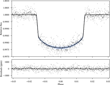
Figure 6. Phase-folded two-minute cadence TESS photometry for HD 1397 from Sector 1. The model generated with the derived parameters of our joint modeling is plotted with a black line. The bottom panel shows the corresponding residuals. For both panels, the gray points represent the relative flux of the TESS photometry and the black points with error bars correspond to the (≈15 minutes) binned flux measurements. The GP component has been removed from the data.
Download figure:
Standard image High-resolution image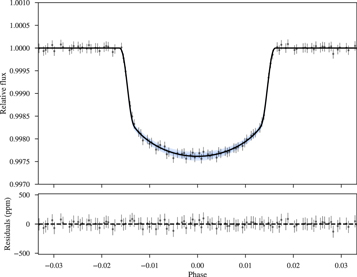
Figure 7. Same as Figure 6, but for the thirty-minute cadence observations of TESS Sector 2.
Download figure:
Standard image High-resolution image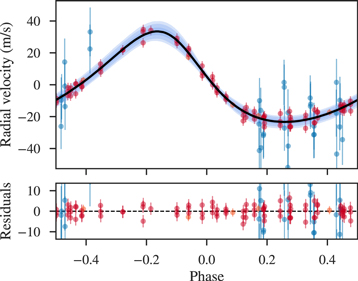
Figure 8. Radial velocities as a function of the orbital phase for HD 1397b obtained with FIDEOS (blue), FEROS (red), and HARPS (orange). The black line represents the model generated from the posterior distributions obtained in Section 3. The error bars include the jitter term obtained from the global analysis. The GP component has been removed from the data.
Download figure:
Standard image High-resolution imageTable 3. Prior and Posterior Parameters of the Global Fit
| Parameter | Prior | Value |
|---|---|---|
| P (days) | N(11.535,0.001) |

|
| T0 (BJD) | N(2458332.0816,0.001) |

|
| a/R⋆ | U(1,300) |

|
| r1a | U(0,1) |

|
| r2a | U(0,1) |

|

|
U(0,1) |

|

|
U(0,1) |

|
 (ppm) (ppm) |
J(1,500) |

|
 (ppm) (ppm) |
J(1,500) |

|
| K (m s−1) | U(0,100) |

|

|
U(−1,1) |

|

|
U(−1,1) |

|
| γFEROS (m s−1) | N(30755,10) |

|
| γHARPS (m s−1) | N(30805,10) |

|
| γFIDEOS(m s−1) | N(30699,10) |

|
| σFEROS (m s−1) | J(0.1,100) |

|
| σHARPS (m s−1) | J(0.1,100) |

|
| σFIDEOS (m s−1) | J(0.1,100) |

|

|

|

|

|

|

|

|

|

|

|

|

|

|

|

|

|

|

|

|

|

|
 (days) (days) |
U(0,1000) |

|
| b |

|
|
 / /
|

|
|
| e |

|
|
| ω (deg) |

|
|
| i (deg) |

|
|
 ( ( ) ) |

|
|
 ( ( ) ) |

|
|
| a (au) |

|
|
 (K)b (K)b
|

|
|
Notes. The derived parameters including the planets physical and orbital properties are presented in the bottom part of the table. For the priors, N(μ, σ) stands for a normal distribution with mean μ and standard deviation σ, U(a, b) stands for a uniform distribution between a and b, and J(a, b) stands for a Jeffrey's prior defined between a and b.
aThese parameters correspond to the parameterization presented in Espinoza (2018) for sampling physically possible combinations of b and /
/ .
bTime-averaged equilibrium temperature computed according to Equation (16) of Méndez & Rivera-Valentín (2017).
.
bTime-averaged equilibrium temperature computed according to Equation (16) of Méndez & Rivera-Valentín (2017).
Download table as: ASCIITypeset image
By combining the results of the global analysis with the physical parameters derived for the stellar host, we find that HD 1397b has a Saturn-like mass of  , but a radius that is more similar to that of Jupiter (
 ). HD 1397b has a semimajor axis of
  , which coupled to its orbital eccentricity results in a distance to the star at periapsis of 0.0786 ±0.0003 au. This orbital configuration also results in an averaged equilibrium temperature for HD 1397b of
  , assuming zero albedo and full energy redistribution. The derived parameters of HD 1397b are listed in Table 3.
4. Discussion
4.1. Structure
HD 1397b adds up to the still sparse, but recently growing, population of transiting giant planets with well-constrained parameters orbiting beyond 0.1 au (see Figure 9). While located relatively far from its host star if compared to the typical population of hot Jupiters, the moderately massive stellar host ( ) is responsible for producing insolation levels on HD 1397b that are high enough (
 ) to possibly alter the internal planetary structure (Kovács et al. 2010; Demory & Seager 2011). Therefore, in terms of structure, HD 1397b shares similar properties to other known low-mass hot Jupiters, like WASP-83b (Hellier et al. 2015), HATS-21b (Bhatti et al. 2016), and WASP-160b (Lendl et al. 2019; see Figure 10).
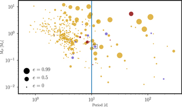
Figure 9. Planet mass vs. orbital period scatter plot for the population of giant transiting planets with masses and radii measured with a precision of 20% or better. The size of the points scales with the orbital eccentricity and the color represents the evolutionary state of the host star (yellow: main-sequence stars, purple: subgiant stars, red: giant stars). The vertical line corresponds to the approximate division between hot and warm Jupiters (10 days). The position of HD 1397b is marked with a square.
Download figure:
Standard image High-resolution image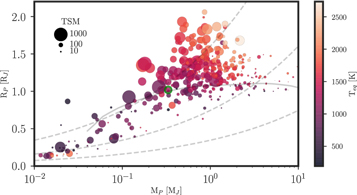
Figure 10. Mass—radius diagram for the population of well-characterized transiting planets. The point corresponding to HD 1397b is marked with a green contour. The color represents the equilibrium temperature of the planet, while the size scales down with the transmission spectroscopy metric as defined by Kempton et al. (2018). The dashed gray lines correspond to isodensity curves for 0.3, 3 and 30 g cm−3, respectively. The solid line corresponds to the predicted radius using the models of Fortney et al. (2007) for a planet with a 10  central core.
Download figure:
Standard image High-resolution image
Regardless of its moderately high equilibrium temperature, the observed physical properties of HD 1397b are still consistent with standard structural models. Specifically, using the models of Fortney et al. (2007), we obtain that given the current stellar age, luminosity, and star–planet separation, the structure of HD 1397b requires the presence of a core of ≈8.3 ± 2.5  of solid material, which is consistent with the values expected in the core accretion model of planet formation (Pollack et al. 1996).
Even though HD 1397b presents a relatively shallow transit depth, the bright host star coupled to the relatively low density of the planet make the HD 1397 system a well-suited target for transmission spectroscopy observations (see Figure 10). Specifically, with a transmission spectroscopy metric (TSM) of TSM = 253, HD 1397b would be ranked in the first quartile for atmospheric characterization as proposed by Kempton et al. (2018). While Figure 10 shows that there are several other planets close to HD 1397b in the  plane that present higher TSM values, HD 1397b remains unique in terms of atmospheric characterization given its long orbital period. HD 1397 along with HD 209458 (Henry et al. 2000) and HD 189733 (Bouchy et al. 2005) are the three brightest systems known to host transiting giant planets.
4.2. Orbital Evolution
The orbital parameters of HD 1397b are well suited for studying the migration mechanism of close-in giant planets. Its current distance to the star during periastron passages is too large for producing significant migration by tidal interactions, and therefore the orbital properties should contain information about the migration history. As an important fraction of other recently discovered transiting warm Jupiters, HD 1397b presents a moderate eccentricity ( ). Eccentricity excitation is expected to be suppressed during the disk lifetime (Dunhill et al. 2013), and therefore the gentle disk migration mechanism is at odds with these observations. Additionally, planet–planet scattering at these short orbital distances should preferentially produce collisions between planets, rather than the excitation of eccentricities12
(Petrovich et al. 2014). Eccentricities of the observed population of warm Jupiters can be enhanced by secular gravitational interactions with other exterior orbiting companions having eccentric and/or highly misaligned orbits (Kozai 1962; Lidov 1962; Naoz 2016). In this scenario the eccentricity and spin–orbit angle of the inner planet suffer periodic variations in timescales significantly larger than the orbital period, and when the eccentricity approaches unity, the planets experiences significant inward migration. Additionally, Dong et al. (2014) predict that the perturber should be close enough in order to overcome the precesion caused by general relativity.
). Eccentricity excitation is expected to be suppressed during the disk lifetime (Dunhill et al. 2013), and therefore the gentle disk migration mechanism is at odds with these observations. Additionally, planet–planet scattering at these short orbital distances should preferentially produce collisions between planets, rather than the excitation of eccentricities12
(Petrovich et al. 2014). Eccentricities of the observed population of warm Jupiters can be enhanced by secular gravitational interactions with other exterior orbiting companions having eccentric and/or highly misaligned orbits (Kozai 1962; Lidov 1962; Naoz 2016). In this scenario the eccentricity and spin–orbit angle of the inner planet suffer periodic variations in timescales significantly larger than the orbital period, and when the eccentricity approaches unity, the planets experiences significant inward migration. Additionally, Dong et al. (2014) predict that the perturber should be close enough in order to overcome the precesion caused by general relativity.
A detailed follow-up characterization of the HD 1397 system could contribute in explaining its origin. While the eccentricity of the planet could be linked with gravitational interactions with other objects in the system, a long-term radial velocity monitoring could clarify if the second signal is indeed an effect of the activity of the star or if it is produced by a nearby planetary companion. Additionally, the measurement of the angle between the spin of the star and the orbital plane through the observation of the Rossiter–McLaughlin effect could further help in constraining the migration mechanism. While the expected amplitude of the Rossiter–McLaughlin effect is relatively small (KRM ≈ 8 m s−1 for an aligned orbit; Gaudi & Winn 2007), the signal should be detectable by a wide range of instruments given the brightness of the host star.
4.3. Evolved Host Star
HD 1397b is a peculiar system due to the evolutionary stage of its host star. Radial velocity surveys have found that close-in giant planets are rare around giant and subgiant stars, if compared to the the occurrence rate on main-sequence stars (e.g., Bowler et al. 2010; Johnson et al. 2010; Jones et al. 2014). Two mechanisms have been invoked to explain this. First, the inferred stellar masses for this sample are systematically higher than those of the giant planets orbiting main-sequence stars, and hence the formation of giant planets at close orbital distances or their migration from beyond the snowline could be prevented due to a shorter lifetime of the protoplanetary disk (e.g., Currie 2009). On the other hand, the scarcity of giant planets orbiting evolved stars could be also produced by the spiral decay of the orbits due to the increase in the strength of stellar tides (e.g., Villaver & Livio 2009; Schlaufman & Winn 2013; Villaver et al. 2014). HD 1397b joins the small group of ≈10 well-characterized transiting systems of giant planets in close-in orbits around subgiant stars (see Figure 9). An important fraction of these close-in systems presents accelerations in their radial velocity curves: Kepler-435b (Almenara et al. 2015), K2-39b (Van Eylen et al. 2016), K2-99b (Smith et al. 2017), and KELT-11b (Pepper et al. 2017). While Knutson et al. (2014) show that 50% of the population of hot Jupiters orbiting main-sequence stars have outer companions, the radial velocity slopes derived for this population are statistically smaller than those present in the population of close-in planets orbiting subgiant stars. These observations indicate that the populations of close-in planets orbiting main-sequence and subgiant stars are probably distinct, where the latter have more massive and/or closer companions. In the forthcoming years, the TESS mission is expected to produce a statistically significant sample of close-in transiting giant planets orbiting evolved stars amenable for detailed dynamical characterization, which will allow further study the of origin of the low occurrence rate of this type of planetary system.
During the reviewing process of this manuscript the discovery of HD 1397b was announced by an independent study (Nielsen et al. 2019).
R.B. acknowledges support from FONDECYT Post-doctoral Fellowship Project 3180246, and from the Millennium Institute of Astrophysics (MAS). A.J. acknowledges support from FONDECYT project 1171208, CONICYT project Basal AFB-170002, and by the Ministry for the Economy, Development, and Tourism's Programa Iniciativa Científica Milenio through grant IC 120009, awarded to the Millennium Institute of Astrophysics (MAS). M.R.D. is supported by CONICYT-PFCHA/Doctorado Nacional-21140646, Chile. J.S.J. acknowledges support by FONDECYT project 1161218 and partial support by BASAL CATA PFB-06. A.Z. acknowledges support by CONICYT-PFCHA/Doctorado Nacional 21170536, Chile. We acknowledge the use of TESS Alert data, which is currently in a beta test phase, from pipelines at the TESS Science Office and at the TESS Science Processing Operations Center. This research has made use of the Exoplanet Follow-up Observation Program website, which is operated by the California Institute of Technology, under contract with the National Aeronautics and Space Administration under the Exoplanet Exploration Program. This paper includes data collected by the TESS mission, which are publicly available from the Mikulski Archive for Space Telescopes (MAST). We thank Sam Kim, Régis Lachaume, and Martin Schlecker for their technical assistance during the observations at the MPG 2.2 m Telescope.
Software: juliet (Espinoza et al. 2018), CERES (Jordán et al. 2014; Brahm et al. 2017a), ZASPE (Brahm et al. 2015, 2017b), radvel (Fulton et al. 2018) emcee (Foreman-Mackey et al. 2013), MultiNest (Feroz et al. 2009) batman (Kreidberg 2015).
Appendix:
Table 4 presents the radial velocity and bisector span measurements of HD 1397 obtained with FEROS, HARPS, and FIDEOS.
Table 4. Relative Radial Velocities and Bisector Spans for HD 1397
| BJD | RV | σRV | BIS | σBIS | S index | σS index | Instrument |
|---|---|---|---|---|---|---|---|
| (km s−1) | (km s−1) | (km s−1) | (km s−1) | ||||
| 2458367.68314629 | 30.7863 | 0.0020 | 0.022 | 0.002 | ⋯ | ⋯ | HARPS |
| 2458368.66398162 | 30.7806 | 0.0020 | 0.021 | 0.002 | ⋯ | ⋯ | HARPS |
| 2458368.68745551 | 30.6687 | 0.007 | −0.013 | 0.006 | ⋯ | ⋯ | FIDEOS |
| 2458368.69912355 | 30.6521 | 0.007 | −0.028 | 0.006 | ⋯ | ⋯ | FIDEOS |
| 2458368.70678972 | 30.6834 | 0.007 | 0.002 | 0.007 | ⋯ | ⋯ | FIDEOS |
| 2458368.75311381 | 30.6773 | 0.007 | −0.032 | 0.007 | ⋯ | ⋯ | FIDEOS |
| 2458368.76041725 | 30.6538 | 0.007 | −0.022 | 0.007 | ⋯ | ⋯ | FIDEOS |
| 2458368.85411697 | 30.6615 | 0.008 | −0.011 | 0.009 | ⋯ | ⋯ | FIDEOS |
| 2458368.86145728 | 30.6624 | 0.008 | −0.034 | 0.008 | ⋯ | ⋯ | FIDEOS |
| 2458369.64418781 | 30.6956 | 0.007 | −0.038 | 0.007 | ⋯ | ⋯ | FIDEOS |
| 2458369.65198892 | 30.6926 | 0.007 | −0.008 | 0.007 | ⋯ | ⋯ | FIDEOS |
| 2458369.65923657 | 30.6669 | 0.007 | −0.037 | 0.007 | ⋯ | ⋯ | FIDEOS |
| 2458369.78679607 | 30.6421 | 0.008 | −0.036 | 0.008 | ⋯ | ⋯ | FIDEOS |
| 2458369.79512629 | 30.6764 | 0.008 | −0.014 | 0.008 | ⋯ | ⋯ | FIDEOS |
| 2458369.80270826 | 30.6555 | 0.008 | −0.029 | 0.008 | ⋯ | ⋯ | FIDEOS |
| 2458370.64460774 | 30.6861 | 0.007 | 0.006 | 0.007 | ⋯ | ⋯ | FIDEOS |
| 2458370.65242178 | 30.6809 | 0.007 | 0.003 | 0.007 | ⋯ | ⋯ | FIDEOS |
| 2458370.66037165 | 30.6822 | 0.007 | 0.005 | 0.007 | ⋯ | ⋯ | FIDEOS |
| 2458370.78118598 | 30.6629 | 0.008 | −0.008 | 0.008 | ⋯ | ⋯ | FIDEOS |
| 2458370.78842912 | 30.6683 | 0.008 | −0.016 | 0.008 | ⋯ | ⋯ | FIDEOS |
| 2458370.79561044 | 30.6631 | 0.008 | 0.005 | 0.008 | ⋯ | ⋯ | FIDEOS |
| 2458371.64189723 | 30.6767 | 0.008 | −0.026 | 0.008 | ⋯ | ⋯ | FIDEOS |
| 2458371.64982610 | 30.6960 | 0.008 | −0.044 | 0.008 | ⋯ | ⋯ | FIDEOS |
| 2458371.65723468 | 30.6510 | 0.014 | 0.025 | 0.014 | ⋯ | ⋯ | FIDEOS |
| 2458371.77405182 | 30.6681 | 0.008 | −0.005 | 0.008 | ⋯ | ⋯ | FIDEOS |
| 2458371.78144230 | 30.6848 | 0.008 | −0.009 | 0.008 | ⋯ | ⋯ | FIDEOS |
| 2458371.78862670 | 30.6807 | 0.008 | −0.019 | 0.008 | ⋯ | ⋯ | FIDEOS |
| 2458371.87779688 | 30.6601 | 0.010 | 0.011 | 0.010 | ⋯ | ⋯ | FIDEOS |
| 2458372.65137095 | 30.6693 | 0.007 | 0.002 | 0.007 | ⋯ | ⋯ | FIDEOS |
| 2458372.65854816 | 30.6858 | 0.007 | −0.018 | 0.007 | ⋯ | ⋯ | FIDEOS |
| 2458372.67407844 | 30.6880 | 0.007 | −0.014 | 0.007 | ⋯ | ⋯ | FIDEOS |
| 2458372.79013200 | 30.7100 | 0.008 | 0.017 | 0.009 | ⋯ | ⋯ | FIDEOS |
| 2458372.79735118 | 30.6948 | 0.008 | 0.005 | 0.009 | ⋯ | ⋯ | FIDEOS |
| 2458372.80462143 | 30.6821 | 0.008 | 0.001 | 0.009 | ⋯ | ⋯ | FIDEOS |
| 2458373.75687607 | 30.7194 | 0.009 | 0.051 | 0.009 | ⋯ | ⋯ | FIDEOS |
| 2458373.76411946 | 30.7301 | 0.009 | 0.015 | 0.009 | ⋯ | ⋯ | FIDEOS |
| 2458379.71952476 | 30.7427 | 0.005 | 0.001 | 0.005 | 0.1963 | 0.0019 | FEROS |
| 2458379.72709860 | 30.7462 | 0.005 | 0.002 | 0.005 | 0.1942 | 0.0018 | FEROS |
| 2458379.73465009 | 30.7490 | 0.005 | 0.001 | 0.005 | 0.1923 | 0.0019 | FEROS |
| 2458383.71877730 | 30.7464 | 0.005 | 0.004 | 0.005 | 0.1905 | 0.0018 | FEROS |
| 2458383.72286419 | 30.7444 | 0.005 | 0.002 | 0.005 | 0.1941 | 0.0018 | FEROS |
| 2458383.72928826 | 30.7401 | 0.005 | 0.001 | 0.005 | 0.2323 | 0.0021 | FEROS |
| 2458384.74720465 | 30.7524 | 0.005 | 0.005 | 0.005 | 0.1940 | 0.0019 | FEROS |
| 2458384.75128807 | 30.7588 | 0.005 | 0.006 | 0.005 | 0.1947 | 0.0019 | FEROS |
| 2458384.75537333 | 30.7585 | 0.005 | 0.002 | 0.005 | 0.1933 | 0.0020 | FEROS |
| 2458385.69639408 | 30.7720 | 0.005 | 0.001 | 0.005 | 0.1890 | 0.0017 | FEROS |
| 2458385.70045388 | 30.7691 | 0.005 | 0.000 | 0.005 | 0.1851 | 0.0018 | FEROS |
| 2458385.70451623 | 30.7669 | 0.005 | 0.001 | 0.005 | 0.1935 | 0.0017 | FEROS |
| 2458398.85664355 | 30.7997 | 0.005 | −0.002 | 0.005 | 0.1852 | 0.0030 | FEROS |
| 2458398.86160055 | 30.7927 | 0.005 | −0.002 | 0.005 | 0.1991 | 0.0038 | FEROS |
| 2458398.86646831 | 30.8011 | 0.005 | 0.006 | 0.005 | 0.1789 | 0.0037 | FEROS |
| 2458401.67766910 | 30.7623 | 0.005 | 0.002 | 0.005 | 0.2000 | 0.0018 | FEROS |
| 2458401.68490538 | 30.7610 | 0.005 | 0.000 | 0.005 | 0.1980 | 0.0017 | FEROS |
| 2458401.68884631 | 30.7641 | 0.005 | 0.006 | 0.005 | 0.1973 | 0.0018 | FEROS |
| 2458404.50796278 | 30.7509 | 0.005 | 0.006 | 0.005 | 0.1955 | 0.0028 | FEROS |
| 2458406.54669111 | 30.7631 | 0.005 | 0.006 | 0.005 | 0.2147 | 0.0025 | FEROS |
| 2458406.55379532 | 30.7593 | 0.005 | 0.005 | 0.005 | 0.2109 | 0.0025 | FEROS |
| 2458406.55921117 | 30.7620 | 0.005 | 0.002 | 0.005 | 0.2151 | 0.0025 | FEROS |
| 2458407.51309835 | 30.7715 | 0.005 | 0.008 | 0.005 | 0.2121 | 0.0026 | FEROS |
| 2458407.51829310 | 30.7741 | 0.005 | 0.004 | 0.005 | 0.2008 | 0.0034 | FEROS |
| 2458407.52382158 | 30.7766 | 0.005 | 0.015 | 0.005 | 0.2121 | 0.0035 | FEROS |
| 2458409.61580549 | 30.8010 | 0.005 | 0.008 | 0.005 | 0.2164 | 0.0020 | FEROS |
| 2458409.62127285 | 30.8011 | 0.005 | 0.003 | 0.005 | 0.2168 | 0.0020 | FEROS |
| 2458410.69117440 | 30.8143 | 0.005 | 0.003 | 0.005 | 0.2107 | 0.0024 | FEROS |
| 2458411.68527663 | 30.8072 | 0.005 | 0.002 | 0.005 | 0.2167 | 0.0020 | FEROS |
| 2458411.68936375 | 30.8089 | 0.005 | 0.005 | 0.005 | 0.2136 | 0.0020 | FEROS |
| 2458411.69344901 | 30.8056 | 0.005 | 0.009 | 0.005 | 0.2176 | 0.0021 | FEROS |
| 2458412.65419276 | 30.7916 | 0.005 | 0.003 | 0.005 | 0.2101 | 0.0016 | FEROS |
| 2458412.65825916 | 30.7853 | 0.005 | 0.004 | 0.005 | 0.2110 | 0.0017 | FEROS |
| 2458412.66232846 | 30.7872 | 0.005 | 0.003 | 0.005 | 0.2101 | 0.0017 | FEROS |
| 2458413.56187674 | 30.7734 | 0.005 | 0.005 | 0.005 | 0.2067 | 0.0015 | FEROS |
| 2458413.56594013 | 30.7713 | 0.005 | 0.004 | 0.005 | 0.2101 | 0.0016 | FEROS |
| 2458413.57000699 | 30.7723 | 0.005 | 0.003 | 0.005 | 0.2073 | 0.0017 | FEROS |
| 2458414.64539175 | 30.7621 | 0.005 | 0.006 | 0.006 | 0.2081 | 0.0019 | FEROS |
| 2458414.64946278 | 30.7646 | 0.005 | 0.007 | 0.006 | 0.2079 | 0.0017 | FEROS |
| 2458414.65458118 | 30.7597 | 0.005 | 0.003 | 0.006 | 0.2087 | 0.0018 | FEROS |
| 2458415.63730889 | 30.7569 | 0.005 | 0.004 | 0.007 | 0.2119 | 0.0020 | FEROS |
| 2458415.64138930 | 30.7544 | 0.005 | 0.004 | 0.006 | 0.2046 | 0.0020 | FEROS |
| 2458415.64547434 | 30.7619 | 0.005 | 0.005 | 0.007 | 0.2072 | 0.0021 | FEROS |
| 2458416.60613278 | 30.7547 | 0.005 | 0.002 | 0.006 | 0.2076 | 0.0016 | FEROS |
| 2458416.61019593 | 30.7487 | 0.005 | 0.003 | 0.006 | 0.2059 | 0.0017 | FEROS |
| 2458416.61426082 | 30.7570 | 0.005 | 0.004 | 0.006 | 0.2040 | 0.0016 | FEROS |
| 2458417.52542561 | 30.7916 | 0.002 | 0.023 | 0.002 | ⋯ | ⋯ | HARPS |
| 2458418.61188680 | 30.7580 | 0.005 | 0.005 | 0.006 | 0.2012 | 0.0015 | FEROS |
| 2458418.61596421 | 30.7608 | 0.005 | 0.004 | 0.006 | 0.2004 | 0.0016 | FEROS |
| 2458418.62002979 | 30.7593 | 0.005 | 0.007 | 0.006 | 0.1996 | 0.0016 | FEROS |
| 2458419.58562321 | 30.7659 | 0.005 | 0.005 | 0.006 | 0.2038 | 0.0017 | FEROS |
| 2458419.58968614 | 30.7663 | 0.005 | 0.001 | 0.006 | 0.2043 | 0.0017 | FEROS |
| 2458419.58156051 | 30.7685 | 0.005 | 0.001 | 0.006 | 0.2015 | 0.0016 | FEROS |
| 2458419.64824552 | 30.8056 | 0.002 | 0.023 | 0.002 | ⋯ | ⋯ | HARPS |
| 2458423.66312999 | 30.8181 | 0.002 | 0.019 | 0.002 | ⋯ | ⋯ | HARPS |
| 2458423.67015000 | 30.7871 | 0.005 | 0.003 | 0.006 | 0.1918 | 0.0040 | FEROS |
| 2458423.67423000 | 30.7883 | 0.005 | 0.003 | 0.006 | 0.1945 | 0.0041 | FEROS |
| 2458423.67830999 | 30.7844 | 0.005 | 0.002 | 0.006 | 0.1882 | 0.0040 | FEROS |
| 2458424.58386000 | 30.7713 | 0.005 | −0.002 | 0.006 | 0.1928 | 0.0039 | FEROS |
| 2458424.58791999 | 30.7661 | 0.005 | 0.000 | 0.006 | 0.1914 | 0.0040 | FEROS |
| 2458424.59198000 | 30.7689 | 0.005 | 0.001 | 0.006 | 0.1885 | 0.0039 | FEROS |
| 2458425.75590000 | 30.7374 | 0.005 | −0.002 | 0.006 | 0.1828 | 0.0042 | FEROS |
| 2458425.76076000 | 30.7408 | 0.005 | −0.002 | 0.006 | 0.1888 | 0.0043 | FEROS |
| 2458425.76481000 | 30.7436 | 0.005 | 0.002 | 0.006 | 0.1883 | 0.0044 | FEROS |
| 2458426.53684000 | 30.7416 | 0.005 | 0.001 | 0.006 | 0.1868 | 0.0040 | FEROS |
| 2458426.54092000 | 30.7420 | 0.005 | −0.001 | 0.006 | 0.1939 | 0.0040 | FEROS |
| 2458426.54501000 | 30.7423 | 0.005 | −0.004 | 0.006 | 0.1861 | 0.0040 | FEROS |
| 2458427.56083999 | 30.7418 | 0.005 | −0.004 | 0.006 | 0.1892 | 0.0040 | FEROS |
| 2458427.56490000 | 30.7356 | 0.005 | 0.000 | 0.006 | 0.1895 | 0.0040 | FEROS |
| 2458427.56895999 | 30.7358 | 0.005 | −0.003 | 0.006 | 0.1857 | 0.0040 | FEROS |
| 2458428.59695000 | 30.7476 | 0.005 | 0.000 | 0.006 | 0.1987 | 0.0040 | FEROS |
| 2458428.60100999 | 30.7480 | 0.005 | 0.002 | 0.006 | 0.1981 | 0.0040 | FEROS |
| 2458428.60539999 | 30.7441 | 0.005 | 0.000 | 0.006 | 0.1960 | 0.0039 | FEROS |
| 2458429.56400999 | 30.7483 | 0.005 | 0.001 | 0.006 | 0.1909 | 0.0040 | FEROS |
| 2458429.56808000 | 30.7459 | 0.005 | −0.001 | 0.006 | 0.1892 | 0.0040 | FEROS |
| 2458429.57214999 | 30.7479 | 0.005 | 0.004 | 0.006 | 0.1898 | 0.0041 | FEROS |
| 2458430.69249999 | 30.7544 | 0.005 | 0.002 | 0.006 | 0.1931 | 0.0041 | FEROS |
| 2458430.69637000 | 30.7574 | 0.005 | 0.000 | 0.006 | 0.1895 | 0.0041 | FEROS |
| 2458430.70044999 | 30.7595 | 0.005 | 0.002 | 0.006 | 0.1963 | 0.0042 | FEROS |
| 2458449.63825999 | 30.7461 | 0.005 | 0.003 | 0.006 | 0.2137 | 0.0040 | FEROS |
| 2458449.64233999 | 30.7485 | 0.005 | 0.002 | 0.006 | 0.2074 | 0.0041 | FEROS |
| 2458449.64641000 | 30.7531 | 0.005 | 0.002 | 0.006 | 0.2082 | 0.0041 | FEROS |
| 2458450.60325000 | 30.7606 | 0.005 | 0.002 | 0.006 | 0.2140 | 0.0040 | FEROS |
| 2458450.60734000 | 30.7509 | 0.005 | 0.000 | 0.006 | 0.2124 | 0.0040 | FEROS |
| 2458450.61140999 | 30.7541 | 0.005 | 0.003 | 0.006 | 0.2155 | 0.0040 | FEROS |
| 2458451.55250000 | 30.7548 | 0.005 | 0.004 | 0.006 | 0.2178 | 0.0041 | FEROS |
| 2458451.55655999 | 30.7629 | 0.005 | 0.000 | 0.006 | 0.2166 | 0.0041 | FEROS |
| 2458451.56062000 | 30.7547 | 0.005 | 0.005 | 0.006 | 0.2096 | 0.0041 | FEROS |
| 2458452.55932000 | 30.7685 | 0.005 | 0.003 | 0.006 | 0.2135 | 0.0041 | FEROS |
| 2458452.56339999 | 30.7672 | 0.005 | 0.000 | 0.006 | 0.2104 | 0.0041 | FEROS |
| 2458452.56657999 | 30.7650 | 0.005 | 0.004 | 0.006 | 0.2151 | 0.0040 | FEROS |
Footnotes
- 10
- 11
- 12
More quantitatively, the collisions largely dominate as the escape velocity of the planet of ∼35 km s−1 is significantly lower than its orbital velocity of ∼100 km s−1.