


Abstract
We present a new complete near-infrared (NIR, JHKs) census of RR Lyrae stars (RRLs) in the globular ω Cen (NGC 5139). We collected 15,472 JHKs images with 4–8 m class telescopes over 15 years (2000–2015) covering a sky area around the cluster center of 60 × 34 arcmin2. These images provided calibrated photometry for 182 out of the 198 cluster RRL candidates with 10 to 60 measurements per band. We also provide new homogeneous estimates of the photometric amplitude for 180 (J), 176 (H) and 174 (Ks) RRLs. These data were supplemented with single-epoch JKs magnitudes from VHS and with single-epoch H magnitudes from 2MASS. Using proprietary optical and NIR data together with new optical light curves (ASAS-SN) we also updated pulsation periods for 59 candidate RRLs. As a whole, we provide JHKs magnitudes for 90 RRab (fundamentals), 103 RRc (first overtones) and one RRd (mixed-mode pulsator). We found that NIR/optical photometric amplitude ratios increase when moving from first overtone to fundamental and to long-period (P > 0.7 days) fundamental RRLs. Using predicted period–luminosity–metallicity relations, we derive a true distance modulus of 13.674 ± 0.008 ± 0.038 mag (statistical error and standard deviation of the median) based on spectroscopic iron abundances, and of 13.698 ± 0.004 ± 0.048 mag based on photometric iron abundances. We also found evidence of possible systematics at the 5%–10% level in the zero-point of the period–luminosity relations based on the five calibrating RRLs whose parallaxes had been determined with the HST.
Export citation and abstract BibTeX RIS
1. Introduction
There is mounting evidence that deep and accurate near-infrared (NIR) photometry presents several indisputable advantages over optical photometry concerning distance determinations. The obvious advantage is the lower sensitivity to reddening (i.e., uncertainties in the reddening values or the presence of differential reddening), but the advantages become even more relevant when dealing with primary distance indicators such as Cepheids (classical and type-II) and RR Lyrae (RRL) stars. Theory and observations indicate that the dispersions of period–luminosity (PL) relations steadily decrease when moving from optical to NIR bands. The PL relations can be derived neglecting the color term, i.e., the width in temperature of the instability strip, and this assumption becomes less severe in the NIR regime.
Here, we will focus on the RRLs. In the optical (BV) bands they typically obey a magnitude versus metallicity relation, and the PL relation becomes evident only for wavelengths longer than the R band (Marconi et al. 2015; Braga et al. 2016). The slope of the PL relation steadily increases from the R- to the J-band and attains an almost constant value for wavelengths longer than 2.2 μm (Madore et al. 2013; Beaton et al. 2016; Neeley et al. 2017). The amplitudes display a similar trend: they attain their largest values in the U band and approach an almost constant value for wavelengths longer than 2.2 μm (Braga et al. 2015; Neeley et al. 2015; M. Marconi et al. 2018, in preparation). This empirical evidence and theoretical considerations both indicate that luminosity variation in the optical regime is mainly dominated by effective temperature variation, while in the NIR regime it is mainly dominated by radius variation (Madore et al. 2013; Bono et al. 2016).
The metallicity dependence of RRLs, in contrast with classical Cepheids, is quite well established. Theory and observations indicate that an increase in metal content makes RRLs fainter. The above evidence makes RRLs key standard candles, and they provide a very promising opportunity to provide an independent calibration of secondary distance indicators and to constrain possible systematics between low-mass/old and intermediate-mass/young distance indicators (Beaton et al. 2016). However, we still lack firm empirical estimates of the zero-point, the slope, and the metallicity dependence of the diagnostics adopted to estimate individual RRL distances.
In this context, cluster RRLs play a crucial role, since we have detailed knowledge of both the age and the chemical composition of their progenitors. In particular, the RRLs in ω Cen appear to be an ideal laboratory, even though we are still lacking solid constraints on the formation and evolution of this peculiar globular. The reasons are as follows.
(a) ω Cen includes almost 200 RRLs and they are almost equally split between fundamental and first overtone pulsators. This suggests that the instability strip is well populated both in the red/cool and in the blue/hot region.
(b) Current empirical evidence indicates that RRLs in ω Cen cover a metallicity range of at least one dex. This makes ω Cen a fundamental testbed to constrain the metallicity dependence, since the depth effects are negligible compared with its distance.
(c) ω Cen hosts at least eight alternative distance indicators: (1) tip of the red giant branch (Bellazzini et al. 2004; Bono et al. 2008); (2) HB luminosity level (VandenBerg et al. 2013); (3) Type II Cepheids (Matsunaga et al. 2006; Navarrete et al. 2017); (4) Miras (Feast 1965); (5) SX Phoenicis variables (McNamara 2000); (6) eclipsing binaries (Thompson et al. 2001); (7) the white dwarf cooling sequence (Ortolani & Rosino 1987; Calamida et al. 2008); (8) an astrometric distance (van de Ven et al. 2006). This provides a unique opportunity to constrain the systematics affecting standard candles that originate from different physical mechanisms.
In spite of the quoted indisputable advantages, the NIR investigations lag when compared with optical ones. Accurate NIR time series data for a significant fraction of ω Cen RRLs were provided for the first time by Del Principe et al. (2006). They adopted NIR time series data collected with SOFI at NTT and provided homogeneous mean JKs magnitudes for 180 variables (114 based on proprietary data: 81 J, 119 Ks images).
More recently, Navarrete et al. (2015, 2017) collected NIR time series data (252 J and 600 Ks images) of ω Cen with the VIRCAM at ESO VISTA telescope. They discovered four new candidate RRLs (two cluster members and two nonmembers). They also provided new mean JKs magnitudes for 187 out of the 198 RRLs. Using NIR PL relations for both RRLs and Type II Cepheids they found a weighted-average true distance modulus to ω Cen of 13.708 ± 0.035 mag.
However, our data sets provide a few key advantages with respect to the quoted literature works: (1) full coverage of light curves in the H band; (2) the possibility to complement our data with proprietary optical data; (3) a better pixel scale that provides a more accurate photometric reduction of blended sources in the central region of the cluster.
Although the cluster and field RRLs have been at the crossroads of an empirical effort of paramount importance (OGLE, CATALINA, Pan-STARRS, VVV) we still lack a detailed analysis of the pulsation properties (photometric amplitudes, topology of the instability strip) of RRL stars in the NIR regime. We are interested in providing a complete NIR census of RRLs in ω Cen as a stepping stone for future developments.
(i) To derive new and accurate NIR (JHKs) template light curves. Future ground-based extremely large telescopes and space telescopes (JWST, EUCLID, WFIRST) will allow us to measure RRLs in Local Volume galaxies. It is plausible to assume that they will allow us to collect only a few random points, so NIR templates are essential to improve the accuracy of the mean magnitudes.
(ii) By taking advantage of the coupling between optical and NIR mean magnitudes, to provide a simultaneous estimate of distance, reddening, and metal content adopting an approach similar to that used by Inno et al. (2016) for classical Cepheids in the Large Magellanic Cloud (LMC).
To accomplish these goals we took advantage of specific NIR (JHKs) time series data collected with SOFI at NTT, with NEWFIRM at CTIO and with FourStar (Persson et al. 2013) at Magellan.
The structure of the paper is as follows. In Section 2 we present the NIR JHKs photometric data sets. In this section we introduce not only the NIR time series, but also show the cluster area covered by different data sets and their NIR color–magnitude diagrams (CMDs). The entire sample of cluster RRLs is presented in Section 3. Sections 3.3 and 3.2 deal with the the phasing of the data (light curves) and with period estimates, while in Section 3.3 we discuss the analytical fits to the light curves and the estimates of both mean magnitudes and photometric amplitudes. The comparison with mean magnitudes available in the literature is discussed in Section 3.4. Section 4.1 introduces the topology of the instability strip both in NIR and in NIR–optical CMDs, while in Section 4.2 we outline the properties of the variables in the luminosity amplitude versus logarithmic period (Bailey diagram) together with optical–NIR and NIR photometric amplitude ratios. In Section 5 we present NIR PL relations and discuss in detail their dependence on the metal content. The new distance determinations to ω Cen, based on NIR PL relations, and the comparison with literature estimates are discussed in Section 6. The summary of the main findings of the current investigation and the future developments of the overall project are outlined in Section 7.
2. NIR Photometric Data Sets
A complete synopsis of our NIR data sets is given in Table 1. The grand total of our images is 15,472: 5102 in J, 4872 in H and 5498 in Ks, collected over 15 years (2000 January–2015 January).
Table 1. Log of the Observations of ω Cen in NIR Bands
| Run | ID | Dates | Telescope | Camera | J | H | Ks | other | multiplex |
|---|---|---|---|---|---|---|---|---|---|
| 1 | giuseppe | 2000 Jan 13–2004 Jun 04 | ESO NTT 3.6 m | SOFI | 109 | ⋯ | 130 | ⋯ | ... |
| 2 | milena | 2004 Jun 03 | ESO NTT 3.6 m | SOFI | 15 | ⋯ | ... | ⋯ | ... |
| 3 | anna | 2005 Apr 02 | ESO NTT 3.6 m | SOFI | 12 | 12 | 36 | ⋯ | ... |
| 4 | calamid | 2007 Apr 03–Jun 03 | ESO VLT 8.0 m | MAD | 6 | ⋯ | 9 | 55 | ... |
| 5 | blanco | 2010 May 24–25 | CTIO 4.0 m | Newfirm | 25 | ⋯ | 52 | ⋯ | 4 |
| 6 | lco1306 | 2013 Jun 25–29 | Magellan 6.5 m | FourStar | 900 | 900 | 900 | ⋯ | 4 |
| 7 | lco1501 | 2015 Jan 26–27 | Magellan 6.5 m | FourStar | 315 | 315 | 365 | ⋯ | 4 |
Notes. 1 ESO program IDs 64.N-0038(A), 66.D-0557(A), 68.D-0545(A), 073.D-0313(A); observer(s) unknown; 2 ESO program ID 073.D-0313(A); observer unknown; 3 ESO program ID 59.A-9004(D); observer unknown; 4 ESO program ID "ID96406"; observer unknown; "other" = Brackett γ; 5 Proposal ID "noao"; observers Allen, DePropris; 6 Observer A. Monson; 7 Observer N. Morrel.
Download table as: ASCIITypeset image
The majority (∼95%) of our data were collected with the FourStar imager (pixel scale: 0.16 arcsec/pix) at the 6.5 m Magellan-Baade telescope at Las Campanas during five nights in 2013 June (10,800 images, Figure 1) and three nights in 2015 January (3979 images, Figure 2; one exposure was missing the data from chip 3). The seeing during the 2013 run was better than 1 2 90% of the time and better than 085 half of the time. Frames from the run of 2015 were collected in excellent seeing conditions: 90% of the time it was better than 06 and, half of the time it was better than 045. The fifteen pointings of the 2013 and 2015 data are almost the same, and cover a sky area of 60 × 34 arcmin2 (∼0.57 degree2). The dithering pattern is made up by five single exposures.
Around 5% of our images were collected with the NEWFIRM instrument (0.4 arcsec/pix) at the CTIO 4.0 m telescope during one night in 2010 May (308 images) and with the SOFI camera (0.25 arcsec/pix) at the NTT 3.6 m telescope at La Silla (314 images) during 2000–2005. Only a few of these data (12 SOFI images) were collected in the H band. These data cover ∼1480 arcmin2 (one NEWFIRM pointing and five SOFI pointings, Figure 3) and are completely contained within the FourStar area. For 90% of the time, the seeing was better than 10, and half of the time better than 07. We point out that the images used by Del Principe et al. (2006) for their photometry are a subsample (200 images) of our SOFI data set.
Finally, we also collected 70 images with MAD at VLT 8.0 m, during 2007 April 3–5 and 2007 June 1 and 3. These data were collected with a seeing of 07–09 but the AO unit of the instrument provided a mean FWHM smaller than 02 for 90% of the images and smaller than 01 for half of the images. The two pointings covered a sky area of 2 arcmin2 (see Figure 4).
As a whole, the entire NIR data set for ω Cen exceeds the capabilities of our computers for simultaneous reduction, so we performed DAOMASTER and ALLFRAME on four independent subsamples: (1) the 2013 June Las Campanas data, hereinafter LCO13; (2) the 2015 January Las Campanas data, hereinafter LCO15; (3) the other natural-seeing observations, hereinafter "other"; (4) AO assisted data, hereinafter MAD. After the completion of the profile-fitting photometry the four catalogs were merged to assign a common numbering scheme to the individual stars.
The photometry was calibrated on the basis of 2MASS stars contained within our images. We considered only 2MASS All-Sky Point Source Catalog photometric measurements that had been assigned photometric quality class "A." This quality class corresponds to magnitude determinations in the J, H, or Ks bandpass with a signal-to-noise ratio ≥10 (σ(magnitude) estimated to be ≤0.109 mag). Matches between the 2MASS stars and entries in our joint catalog were determined by astrometric agreement within a tolerance of 1 arcsec; matches satisfying this criterion agreed positionally with a standard deviation of 0.15 arcsec in the x (∼right ascension) direction and 0.14 arcsec in y (∼declination). The 2MASS magnitudes were used as standard measurements to calibrate our instrumental magnitudes using transformation equations employing linear color terms. Individual stars displaying large residuals from preliminary fits were gradually discarded until the transformation relied only on 12,802 individual 2MASS stars with fitting residuals <0.20 mag in at least one of the three bandpasses.
Our natural-seeing observations of ω Cen were calibrated to the 2MASS photometric system on the basis of these transformation equations. An additional 172 fainter but well-isolated stars that were well-observed in our data sets were selected to serve as secondary calibrators for the MAD observations.
In reducing the NIR data set for ω Cen we adopted a double strategy. We performed ALLSTAR/ALLFRAME photometry over the entire set of NIR images. This approach is required to have accurate time series data to estimate the pulsation parameters.
Moreover, we also performed an independent photometric reduction based upon the stacked images. This approach was adopted to improve the detection of faint stars and to provide a very accurate and deep NIR (JHKs) catalog, with no attempt at time resolution.
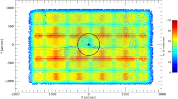
Figure 1. Distribution on the sky (arcseconds) of the photometry performed on NIR (JHKs) images collected with FourStar at Magellan in 2013 (LCO13). This data set covers a cluster area of 60 × 34 arcmin2. The color coding is correlated with the number of measurements (see the right bar). A black plus marks the position of the cluster center (Braga et al. 2016). The black circle marks the half-mass radius (300 arcsec; Harris 1996).
Download figure:
Standard image High-resolution image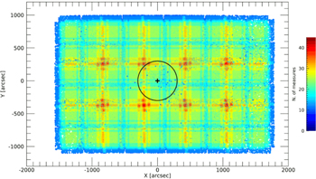
Figure 2. Same as in Figure 1, but for NIR (JHKs) images collected with FourStar at Magellan in 2015 (LCO15). This data set covers a cluster area of 60 × 34 arcmin2.
Download figure:
Standard image High-resolution image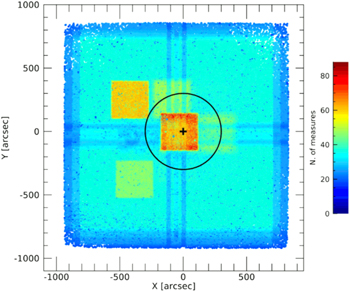
Figure 3. Same as in Figure 1, but for NIR (JHKs) images collected with different telescopes ("other" data set, see text for more details). This data set covers a cluster area of 27 × 33 arcmin2.
Download figure:
Standard image High-resolution image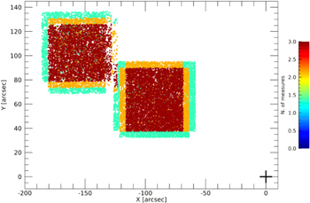
Figure 4. Same as in Figure 1, but for NIR (JKs) images collected with the MCAO system (MAD) that was available at VLT. The individual pointings cover an area of 1 × 1 arcmin2.
Download figure:
Standard image High-resolution imageWe have derived accurate CMDs from the current photometry, covering both the bright region typical of red giant branch (RGB) and asymptotic giant branch stars (up to Ks ∼ 8.5 mag thanks to the SOFI data), but also ∼1.5–2.5 magnitudes fainter than the main sequence turn-off region (FourStar data, see Figure 5). The mean squared sums of the J- and Ks-band photometric errors in different magnitude bins are plotted as red error bars on the right of each panel.
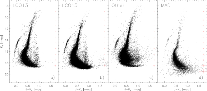
Figure 5. NIR (Ks vs. J–Ks) color–magnitude diagrams of ω Cen. Error bars display intrinsic errors both in magnitude and in color. To make them visible, they are magnified by a factor of five.
Download figure:
Standard image High-resolution imageThe stars plotted in the above CMDs have been selected by the χ parameter, which quantifies the deviation between the star profile and the adopted point-spread function (PSF), and the sharpness ( < 0.7), which indicates the difference in broadness of the individual stars compared with the PSF and is used to reject non-stellar sources. In passing we note that PSF photometry of individual images is essential to improve the precision of individual measurements of variable stars. The identification and fitting of faint sources located near the variable stars provides an optimal subtraction of light contamination from neighboring stars.
The effect of seeing is clear when we compare the CMDs in panels (a) and (b): the telescope and the camera are the same, but the better seeing during 2015 allowed us to gain ∼0.3 mag in depth. However, the better seeing also caused a larger spread in color of stars on the upper RGB (Ks < 12 mag), due to a fainter level of saturation.
The effect of the seeing and of the pixel scale of the instrument is also clear when comparing the LCO13, LCO15 and other data sets. LCO15 is, in fact, ∼0.3 mag deeper than the other two and that with the least populated RGB and the sharpest blue and extreme horizontal branch. On the other hand, the other data set has a better populated upper RGB.
Finally, the MAD data set is the deepest, but most importantly, shows the least amount of contamination by field stars—which is quite clear in the two LCO data sets at J–Ks ∼ 0.85 mag—since the observed sky area is small and very close to the cluster center. These are clear advantages of using AO corrections for the CMD observations (but an obvious disadvantage for acquiring a large sample of RR Lyraes).
3. RR Lyrae Stars
We adopt Table 2 in Braga et al. (2016) as our reference list of RRL candidates in ω Cen, but exclude NV433 as suggested by Navarrete et al. (2015). Note that we use the term "RRL candidates" because we lack solid, homogeneous constraints on their membership, other than considerations on their distance from the cluster center, mean magnitude, and proper motions for a few of them (van Leeuwen et al. 2000; Bellini et al. 2009). Therefore, we kept 198 out of 199 objects from the quoted list. According to the literature, eight of these 198 stars are confirmed nonmembers (V84, V168, V175, V181, V183, V283, NV457, NV458, van Leeuwen et al. 2000; Fernández-Trincado et al. 2015; Navarrete et al. 2015). The classification of V68 and V84 is ambiguous because, until now, their periods and their positions in both the CMD and in the period–magnitude plane did not allow a clear discrimination between RRL and anomalous Cepheid (AC) classifications. For three stars (V171, V178 and V179) neither periods nor mean magnitudes were available, while for V182, only the period was known. However, for the first time since these four stars were classified as variables (Wilkens 1965; Sawyer Hogg 1973), we have retrieved multi-epoch photometry for them. Thus, we have data for all the RRL candidates of ω Cen.
For the master catalog for the ALLFRAME runs on our NIR data, we adopted the catalog generated during the photometric reduction of the optical (UBVRI) data (see Section 2 of Braga et al. 2016). This allowed us to assign to the NIR point sources the same identification numbers as the optical sources, providing an unambiguous identification of all the stars within the sky area covered by our images and an accurate cross-match of the optical and NIR catalogs. The cross-match allowed us to retrieve the UBVRI light curves of NV411, that we had missed in Braga et al. (2016).
3.1. Light Curves
The median number of phase points in the light curves obtained from our NIR data is 109, 77, and 136 for the J, H, and Ks bands, respectively. The median of the photometric errors on the single-epoch magnitudes are 0.012, 0.013, and 0.018 mag (J, H, and Ks). However, there is a large difference in the photometric errors between the FourStar data (median ≲0.015 mag in the JHKs bands) and the data sets blanco and milena (subsets of the other data set, Table 1, median ≳0.025 mag in all bands); moreover, errors on the single phase points can be as large as 0.2 mag.
As a preliminary step before analyzing the light curves, we binned the phase points to combine data from the same dithering sequence. The time step was ∼90 s for the LCO dithering sequence and ∼900 s for the other data. We tested different binning methods, including simple intensity mean, median, and weighted intensity mean. We adopted the weighted intensity mean because it provides smoother light curves. Note that, before averaging the single phase points, we performed a sigma clipping at a 3σ level to reject the outliers. The rejected phase points were probably obtained from images with either a lower quality or for which the photometric solution was not optimal. The fraction of phase points that was rejected in this step was smaller than 5%.
Note that the binning of the data was applied to the dithering sequences of individual data sets. The duration of a dithering sequence is a tiny fraction of the pulsation period of an RRL. Moreover, the bulk of the NIR data were collected as time series data, therefore, possible changes in the pulsation period minimally affect the binning of the data. After the binning process, we ended up with light curves including a median number of phase points of 25 (J), 17 (H) and 30 (Ks), respectively.
3.2. Pulsation Periods
We have already mentioned in Section 2 that the majority of our NIR data were collected in 2013 and 2015. On the other hand, most of the optical time-series data were collected between 1995 and 1999. The remarkable overall time coverage (27 years) of optical plus NIR data allowed us to revise the period estimates derived in Braga et al. (2016). We have derived the new period estimates by adopting the same method as the quoted paper, based on the Lomb–Scargle periodogram (Scargle 1982). This method simultaneously folds the time series of all the photometric bands that are available. A visual inspection of the folded light curves and a quantitative estimate of the χ2 allow us to estimate the period. On the basis of our overall optical and NIR photometry, we provide new period estimates for 59 variables. For 17 of them, the new period estimate should be considered as an improvement of the estimate based only on the optical data. For 30 variables, the new estimate suggests an intrinsic period change occurred during the time that passed between the acquisition of the bulk of the optical and NIR data (as indicated in Table 2). For the remaining 12 variables, the period available in the literature was updated. Note that V171 and V179 had no period at all in the literature.
Table 2. NIR–JHKs–Mean Magnitudes and Amplitudes for ω Cen RRLs
| ID | Period (new) | Period (old)a | Variable | fitJb | J | AJ | fitHb | H | AH | fitKsb | Ks | AKs |
|---|---|---|---|---|---|---|---|---|---|---|---|---|
| days | days | type | mag | mag | mag | mag | mag | mag | ||||
| V3 | 0.84126158 | ⋯ | RRab | P | 13.182 ± 0.007 | 0.353 ± 0.029 | P | 12.895 ± 0.007 | 0.300 ± 0.029 | S | 12.864 ± 0.009 | 0.285 ± 0.027 |
| V4 | 0.62731846 | ⋯ | RRab | S | 13.378 ± 0.008 | 0.494 ± 0.054 | S | 13.106 ± 0.008 | 0.333 ± 0.031 | S | 13.077 ± 0.009 | 0.316 ± 0.020 |
| V5c | 0.51528002 | ⋯ | RRab | S | 13.668 ± 0.012 | 0.441 ± 0.028 | S | 13.488 ± 0.019 | 0.354 ± 0.043 | S | 13.409 ± 0.012 | 0.334 ± 0.016 |
| V7 | 0.71303420 | ⋯ | RRab | S | 13.289 ± 0.005 | 0.428 ± 0.041 | P | 13.018 ± 0.006 | 0.305 ± 0.025 | S | 12.976 ± 0.006 | 0.312 ± 0.028 |
| V8 | 0.52132593 | ⋯ | RRab | S | 13.577 ± 0.004 | 0.449 ± 0.056 | S | 13.341 ± 0.009 | 0.344 ± 0.018 | S | 13.305 ± 0.005 | 0.295 ± 0.017 |
| V9c | 0.52335114d | 0.52346446 | RRab | S | 13.641 ± 0.010 | 0.320 ± 0.050 | P | 13.430 ± 0.005 | 0.175 ± 0.033 | S | 13.378 ± 0.009 | 0.225 ± 0.025 |
| V10 | 0.37475609e | 0.37488161 | RRc | P | 13.551 ± 0.006 | 0.153 ± 0.013 | S | 13.316 ± 0.017 | ⋯ | S | 13.313 ± 0.009 | 0.080 ± 0.010 |
| V11c | 0.56480650 | ⋯ | RRab | S | 13.474 ± 0.005 | 0.248 ± 0.023 | S | 13.209 ± 0.008 | 0.189 ± 0.023 | S | 13.189 ± 0.006 | 0.196 ± 0.016 |
| V12 | 0.38677657d | 0.38676730 | RRc | S | 13.545 ± 0.011 | ⋯ | S | 13.299 ± 0.015 | ⋯ | S | 13.281 ± 0.010 | ... |
| V13 | 0.66904841 | ⋯ | RRab | S | 13.315 ± 0.008 | 0.405 ± 0.026 | S | 13.039 ± 0.008 | 0.330 ± 0.028 | S | 13.011 ± 0.008 | 0.307 ± 0.015 |
| V14 | 0.37710263e | 0.37712562 | RRc | S | 13.575 ± 0.003 | 0.205 ± 0.018 | S | 13.352 ± 0.005 | 0.113 ± 0.011 | P | 13.347 ± 0.005 | 0.110 ± 0.009 |
| V15 | 0.81065426 | ⋯ | RRab | S | 13.178 ± 0.006 | 0.353 ± 0.024 | S | 12.843 ± 0.008 | 0.309 ± 0.033 | S | 12.850 ± 0.007 | 0.287 ± 0.037 |
| V16 | 0.33019610 | ⋯ | RRc | P | 13.688 ± 0.003 | 0.182 ± 0.015 | P | 13.468 ± 0.005 | 0.072 ± 0.009 | S | 13.481 ± 0.004 | 0.103 ± 0.010 |
| V18 | 0.62168636 | ⋯ | RRab | P | 13.421 ± 0.007 | 0.525 ± 0.021 | S | 13.137 ± 0.008 | 0.246 ± 0.014 | S | 13.127 ± 0.007 | 0.323 ± 0.017 |
| V19 | 0.29955165 | ⋯ | RRc | P | 13.864 ± 0.004 | 0.169 ± 0.017 | P | 13.661 ± 0.004 | 0.088 ± 0.010 | S | 13.653 ± 0.005 | 0.111 ± 0.009 |
| V20 | 0.61558779e | 0.61556372 | RRab | S | 13.438 ± 0.014 | 0.426 ± 0.038 | S | 13.114 ± 0.007 | 0.261 ± 0.021 | S | 13.100 ± 0.007 | 0.311 ± 0.019 |
| V21 | 0.38080948 | ⋯ | RRc | S | 13.553 ± 0.009 | 0.198 ± 0.023 | S | 13.369 ± 0.008 | 0.118 ± 0.013 | S | 13.370 ± 0.009 | 0.110 ± 0.015 |
| V22c | 0.39616527d | 0.39608414 | RRc | S | 13.536 ± 0.005 | 0.174 ± 0.014 | S | 13.292 ± 0.008 | 0.120 ± 0.012 | S | 13.289 ± 0.006 | 0.115 ± 0.012 |
| V23 | 0.51087033 | ⋯ | RRab | S | 13.717 ± 0.005 | 0.441 ± 0.054 | P | 13.445 ± 0.010 | ⋯ | S | 13.396 ± 0.008 | 0.357 ± 0.029 |
| V24 | 0.46222155 | ⋯ | RRc | P | 13.396 ± 0.005 | 0.162 ± 0.015 | S | 13.125 ± 0.008 | 0.120 ± 0.013 | S | 13.123 ± 0.006 | 0.093 ± 0.013 |
| V25 | 0.58851546e | 0.58835430 | RRab | S | 13.458 ± 0.009 | 0.437 ± 0.054 | S | 13.194 ± 0.008 | 0.364 ± 0.045 | S | 13.157 ± 0.012 | 0.293 ± 0.029 |
| V26 | 0.78472145 | ⋯ | RRab | S | 13.222 ± 0.005 | 0.317 ± 0.027 | P | 12.927 ± 0.007 | 0.276 ± 0.024 | S | 12.875 ± 0.006 | 0.230 ± 0.020 |
| V27 | 0.61569276 | ⋯ | RRab | S | 13.528 ± 0.003 | 0.237 ± 0.021 | P | 13.220 ± 0.008 | 0.210 ± 0.027 | S | 13.198 ± 0.006 | 0.248 ± 0.020 |
| V30c | 0.40397132e | 0.40423516 | RRc | P | 13.521 ± 0.006 | 0.151 ± 0.009 | S | 13.263 ± 0.009 | 0.073 ± 0.011 | S | 13.246 ± 0.008 | 0.105 ± 0.013 |
| V32c | 0.62036776 | ⋯ | RRab | S | 13.463 ± 0.004 | 0.388 ± 0.030 | S | 13.167 ± 0.006 | 0.321 ± 0.027 | S | 13.119 ± 0.006 | 0.322 ± 0.019 |
| V33 | 0.60233332 | ⋯ | RRab | S | 13.409 ± 0.005 | 0.468 ± 0.045 | S | 13.146 ± 0.010 | 0.315 ± 0.026 | S | 13.141 ± 0.006 | 0.288 ± 0.021 |
| V34 | 0.73395501 | ⋯ | RRab | S | 13.256 ± 0.007 | 0.325 ± 0.029 | S | 12.967 ± 0.005 | 0.248 ± 0.020 | S | 12.931 ± 0.007 | 0.281 ± 0.019 |
| V35 | 0.38683322 | ⋯ | RRc | S | 13.530 ± 0.007 | 0.175 ± 0.013 | P | 13.283 ± 0.008 | 0.134 ± 0.015 | P | 13.290 ± 0.008 | 0.097 ± 0.012 |
| V36 | 0.37990927e | 0.37981328 | RRc | P | 13.529 ± 0.004 | 0.188 ± 0.015 | S | 13.305 ± 0.008 | 0.113 ± 0.011 | S | 13.295 ± 0.004 | 0.112 ± 0.015 |
| V38c | 0.77905902 | ⋯ | RRab | S | 13.219 ± 0.003 | ⋯ | S | 12.916 ± 0.006 | 0.185 ± 0.014 | S | 12.886 ± 0.005 | 0.214 ± 0.015 |
| V39 | 0.39338605 | ⋯ | RRc | P | 13.570 ± 0.005 | 0.179 ± 0.015 | P | 13.328 ± 0.007 | 0.112 ± 0.011 | S | 13.320 ± 0.007 | 0.117 ± 0.010 |
| V40 | 0.63409776 | ⋯ | RRab | S | 13.407 ± 0.006 | 0.489 ± 0.061 | S | 13.129 ± 0.008 | 0.313 ± 0.031 | S | 13.095 ± 0.009 | 0.319 ± 0.029 |
| V41 | 0.66293383 | ⋯ | RRab | S | 13.374 ± 0.007 | 0.381 ± 0.027 | S | 13.082 ± 0.007 | 0.339 ± 0.028 | P | 13.043 ± 0.009 | 0.328 ± 0.019 |
| V44 | 0.56753783d | 0.56753608 | RRab | S | 13.610 ± 0.005 | 0.456 ± 0.044 | S | 13.326 ± 0.006 | 0.306 ± 0.030 | S | 13.304 ± 0.007 | 0.300 ± 0.020 |
| V45c | 0.58913452 | ⋯ | RRab | S | 13.427 ± 0.005 | 0.545 ± 0.082 | S | 13.178 ± 0.003 | 0.323 ± 0.040 | S | 13.161 ± 0.005 | 0.336 ± 0.024 |
| V46 | 0.68696236 | ⋯ | RRab | P | 13.325 ± 0.003 | 0.415 ± 0.045 | S | 13.040 ± 0.003 | 0.288 ± 0.021 | P | 13.016 ± 0.005 | 0.274 ± 0.016 |
| V47 | 0.48532643d | 0.48529500 | RRc | P | 13.320 ± 0.004 | 0.157 ± 0.016 | S | 13.077 ± 0.010 | 0.097 ± 0.016 | P | 13.067 ± 0.007 | 0.101 ± 0.013 |
| V49 | 0.60464946d | 0.60464471 | RRab | S | 13.474 ± 0.003 | 0.422 ± 0.040 | S | 13.197 ± 0.005 | 0.273 ± 0.027 | P | 13.163 ± 0.005 | 0.282 ± 0.016 |
| V50 | 0.38616585 | ⋯ | RRc | S | 13.591 ± 0.004 | 0.186 ± 0.020 | S | 13.343 ± 0.007 | 0.123 ± 0.014 | P | 13.343 ± 0.005 | 0.091 ± 0.011 |
| V51 | 0.57414241 | ⋯ | RRab | S | 13.466 ± 0.006 | 0.414 ± 0.040 | P | 13.179 ± 0.009 | 0.312 ± 0.021 | S | 13.161 ± 0.008 | 0.326 ± 0.020 |
| V52 | 0.66038704 | ⋯ | RRab | S | 13.298 ± 0.016 | 0.468 ± 0.039 | S | 13.060 ± 0.011 | ⋯ | S | 12.977 ± 0.012 | 0.262 ± 0.022 |
| V54 | 0.77290930 | ⋯ | RRab | P | 13.232 ± 0.004 | 0.308 ± 0.033 | S | 12.917 ± 0.005 | 0.281 ± 0.035 | P | 12.884 ± 0.004 | 0.253 ± 0.032 |
| V55 | 0.58166391e | 0.58192068 | RRab | S | 13.614 ± 0.004 | 0.410 ± 0.036 | P | 13.283 ± 0.108 | ⋯ | S | 13.291 ± 0.005 | 0.250 ± 0.015 |
| V56c | 0.56803579 | ⋯ | RRab | S | 13.642 ± 0.008 | 0.425 ± 0.039 | S | 13.346 ± 0.008 | 0.280 ± 0.021 | S | 13.343 ± 0.006 | 0.263 ± 0.018 |
| V57 | 0.79442230 | ⋯ | RRab | S | 13.213 ± 0.003 | 0.269 ± 0.018 | S | 12.887 ± 0.005 | 0.204 ± 0.020 | S | 12.874 ± 0.004 | 0.230 ± 0.015 |
| V58 | 0.37985623e | 0.36992250 | RRc | S | 13.581 ± 0.007 | ⋯ | P | 13.385 ± 0.011 | ⋯ | P | 13.370 ± 0.008 | ... |
| V59c | 0.51855138 | ⋯ | RRab | S | 13.624 ± 0.017 | 0.385 ± 0.066 | P | 13.397 ± 0.013 | 0.312 ± 0.055 | T | 13.39 ± 0.01 | ... |
| V62 | 0.61979638 | ⋯ | RRab | S | 13.398 ± 0.008 | 0.457 ± 0.058 | S | 13.134 ± 0.006 | 0.369 ± 0.040 | S | 13.078 ± 0.007 | 0.288 ± 0.024 |
| V63 | 0.82595979 | ⋯ | RRab | S | 13.190 ± 0.003 | 0.228 ± 0.022 | S | 12.876 ± 0.004 | 0.210 ± 0.021 | S | 12.849 ± 0.004 | 0.199 ± 0.020 |
| V64 | 0.34444598d | 0.34447428 | RRc | S | 13.634 ± 0.005 | 0.195 ± 0.018 | S | 13.409 ± 0.005 | 0.133 ± 0.013 | P | 13.413 ± 0.006 | 0.106 ± 0.012 |
| V66 | 0.40723082d | 0.40727290 | RRc | S | 13.481 ± 0.006 | 0.163 ± 0.015 | S | 13.239 ± 0.006 | 0.113 ± 0.014 | S | 13.230 ± 0.006 | 0.097 ± 0.009 |
| V67c | 0.56444856 | ⋯ | RRab | S | 13.593 ± 0.004 | 0.506 ± 0.048 | S | 13.323 ± 0.006 | 0.326 ± 0.029 | S | 13.310 ± 0.005 | 0.298 ± 0.019 |
| V68 | 0.53462524e | 0.53476174 | RRc/ACep | S | 13.211 ± 0.006 | 0.124 ± 0.012 | P | 12.958 ± 0.007 | 0.053 ± 0.011 | S | 12.942 ± 0.005 | 0.062 ± 0.007 |
| V69c | 0.65322088 | ⋯ | RRab | S | 13.399 ± 0.004 | 0.376 ± 0.033 | S | 13.114 ± 0.006 | 0.273 ± 0.022 | S | 13.099 ± 0.004 | 0.272 ± 0.023 |
| V70 | 0.39081066e | 0.39059068 | RRc | S | 13.517 ± 0.005 | 0.179 ± 0.028 | P | 13.275 ± 0.006 | 0.125 ± 0.017 | S | 13.268 ± 0.005 | 0.102 ± 0.011 |
| V71 | 0.35769621d | 0.35764894 | RRc | S | 13.624 ± 0.019 | ⋯ | P | 13.410 ± 0.010 | ⋯ | S | 13.385 ± 0.012 | ... |
| V72 | 0.38450448 | ⋯ | RRc | S | 13.545 ± 0.004 | 0.181 ± 0.013 | P | 13.303 ± 0.008 | 0.130 ± 0.019 | S | 13.318 ± 0.005 | 0.102 ± 0.010 |
| V73c | 0.57520367 | ⋯ | RRab | S | 13.489 ± 0.004 | 0.449 ± 0.048 | P | 13.236 ± 0.007 | 0.309 ± 0.027 | P | 13.210 ± 0.009 | 0.271 ± 0.025 |
| V74c | 0.50321425 | ⋯ | RRab | S | 13.604 ± 0.005 | 0.544 ± 0.048 | S | 13.379 ± 0.014 | 0.313 ± 0.035 | S | 13.354 ± 0.007 | 0.338 ± 0.038 |
| V75 | 0.42220668e | 0.42214238 | RRc | P | 13.424 ± 0.004 | 0.169 ± 0.015 | P | 13.159 ± 0.006 | 0.128 ± 0.015 | S | 13.164 ± 0.004 | 0.119 ± 0.010 |
| V76 | 0.33796008 | ⋯ | RRc | P | 13.636 ± 0.007 | 0.171 ± 0.020 | P | 13.422 ± 0.009 | ⋯ | T | 13.47 ± 0.01 | ... |
| V77 | 0.42598243e | 0.42604092 | RRc | S | 13.448 ± 0.003 | 0.171 ± 0.022 | S | 13.190 ± 0.006 | 0.099 ± 0.012 | S | 13.184 ± 0.006 | 0.099 ± 0.012 |
| V79 | 0.60828692 | ⋯ | RRab | S | 13.461 ± 0.004 | 0.469 ± 0.041 | S | 13.205 ± 0.011 | 0.325 ± 0.026 | S | 13.152 ± 0.007 | 0.306 ± 0.021 |
| V80 | 0.37719716e | 0.37721794 | RRc | S | 13.633 ± 0.005 | 0.143 ± 0.016 | P | 13.452 ± 0.009 | 0.086 ± 0.015 | S | 13.440 ± 0.009 | 0.083 ± 0.018 |
| V81 | 0.38938509 | ⋯ | RRc | S | 13.535 ± 0.004 | 0.177 ± 0.013 | S | 13.300 ± 0.008 | 0.099 ± 0.014 | S | 13.285 ± 0.006 | 0.110 ± 0.009 |
| V82c | 0.33576546 | ⋯ | RRc | P | 13.591 ± 0.004 | 0.165 ± 0.015 | S | 13.381 ± 0.005 | 0.106 ± 0.012 | P | 13.386 ± 0.007 | 0.092 ± 0.013 |
| V83 | 0.35661021 | ⋯ | RRc | P | 13.602 ± 0.004 | 0.184 ± 0.018 | S | 13.377 ± 0.006 | 0.125 ± 0.016 | P | 13.377 ± 0.005 | 0.106 ± 0.015 |
| V84 | 0.57991785 | ⋯ | RRab/ACep | S | 13.095 ± 0.006 | 0.303 ± 0.027 | S | 12.804 ± 0.008 | 0.232 ± 0.021 | S | 12.781 ± 0.009 | 0.226 ± 0.022 |
| V85 | 0.74274920 | ⋯ | RRab | S | 13.314 ± 0.005 | 0.304 ± 0.025 | S | 12.997 ± 0.009 | 0.290 ± 0.022 | P | 12.957 ± 0.007 | 0.228 ± 0.019 |
| V86 | 0.64784141 | ⋯ | RRab | S | 13.379 ± 0.006 | 0.430 ± 0.053 | S | 13.075 ± 0.006 | 0.386 ± 0.048 | P | 13.051 ± 0.008 | 0.290 ± 0.024 |
| V87 | 0.39594092 | ⋯ | RRc | S | 13.523 ± 0.007 | 0.149 ± 0.018 | S | 13.282 ± 0.012 | 0.081 ± 0.017 | S | 13.249 ± 0.011 | 0.087 ± 0.015 |
| V88 | 0.69021146 | ⋯ | RRab | P | 13.373 ± 0.014 | 0.450 ± 0.044 | S | 13.119 ± 0.026 | 0.289 ± 0.041 | P | 13.049 ± 0.018 | 0.258 ± 0.036 |
| V89 | 0.37403725e | 0.37417885 | RRc | S | 13.576 ± 0.008 | 0.177 ± 0.017 | P | 13.316 ± 0.008 | 0.116 ± 0.014 | S | 13.276 ± 0.012 | 0.123 ± 0.019 |
| V90 | 0.60340531 | ⋯ | RRab | S | 13.420 ± 0.016 | 0.545 ± 0.069 | P | 13.194 ± 0.012 | 0.370 ± 0.030 | P | 13.102 ± 0.010 | 0.274 ± 0.017 |
| V91 | 0.89522178 | ⋯ | RRab | P | 13.086 ± 0.013 | 0.316 ± 0.019 | S | 12.754 ± 0.010 | 0.238 ± 0.019 | S | 12.722 ± 0.010 | 0.257 ± 0.018 |
| V94c | 0.25393406 | ⋯ | RRc | S | 13.987 ± 0.009 | 0.106 ± 0.014 | S | 13.808 ± 0.009 | 0.076 ± 0.015 | P | 13.830 ± 0.008 | 0.053 ± 0.009 |
| V95 | 0.40496622 | ⋯ | RRc | P | 13.501 ± 0.002 | 0.198 ± 0.016 | S | 13.250 ± 0.004 | 0.122 ± 0.014 | S | 13.258 ± 0.004 | 0.118 ± 0.013 |
| V96 | 0.62452166d | 0.62452829 | RRab | S | 13.354 ± 0.014 | 0.365 ± 0.028 | S | 13.094 ± 0.008 | 0.241 ± 0.023 | S | 13.033 ± 0.008 | 0.309 ± 0.023 |
| V97c | 0.69188985 | ⋯ | RRab | S | 13.321 ± 0.005 | 0.417 ± 0.026 | S | 13.022 ± 0.009 | 0.308 ± 0.021 | S | 12.995 ± 0.008 | 0.280 ± 0.016 |
| V98 | 0.28056563 | ⋯ | RRc | S | 13.916 ± 0.008 | 0.196 ± 0.021 | S | 13.716 ± 0.012 | 0.120 ± 0.021 | S | 13.725 ± 0.011 | 0.094 ± 0.011 |
| V99 | 0.76617945 | ⋯ | RRab | S | 13.172 ± 0.009 | 0.454 ± 0.035 | S | 12.892 ± 0.014 | 0.332 ± 0.081 | S | 12.854 ± 0.009 | 0.247 ± 0.018 |
| V100 | 0.55274773 | ⋯ | RRab | S | 13.631 ± 0.006 | 0.502 ± 0.062 | S | 13.341 ± 0.013 | 0.294 ± 0.027 | S | 13.329 ± 0.008 | 0.299 ± 0.021 |
| V101 | 0.34099950e | 0.34094664 | RRc | S | 13.655 ± 0.006 | 0.120 ± 0.017 | S | 13.434 ± 0.006 | 0.038 ± 0.008 | S | 13.443 ± 0.006 | 0.046 ± 0.011 |
| V102 | 0.69139606 | ⋯ | RRab | S | 13.329 ± 0.004 | 0.453 ± 0.044 | S | 13.030 ± 0.006 | ⋯ | S | 12.993 ± 0.006 | 0.290 ± 0.017 |
| V103 | 0.32885556 | ⋯ | RRc | S | 13.643 ± 0.008 | ⋯ | S | 13.441 ± 0.007 | 0.078 ± 0.010 | S | 13.426 ± 0.007 | ... |
| V104 | 0.86752592e | 0.86656711 | RRab | S | 13.217 ± 0.011 | 0.174 ± 0.015 | S | 12.884 ± 0.010 | 0.199 ± 0.017 | P | 12.856 ± 0.011 | 0.168 ± 0.014 |
| V105 | 0.33533089 | ⋯ | RRc | P | 13.756 ± 0.003 | 0.168 ± 0.016 | S | 13.530 ± 0.004 | 0.122 ± 0.011 | S | 13.534 ± 0.004 | 0.107 ± 0.010 |
| V106c | 0.56990293 | ⋯ | RRab | P | 13.465 ± 0.011 | 0.513 ± 0.048 | P | 13.230 ± 0.020 | 0.301 ± 0.052 | T | 13.17 ± 0.01 | ... |
| V107 | 0.51410378 | ⋯ | RRab | S | 13.658 ± 0.008 | 0.446 ± 0.033 | S | 13.407 ± 0.006 | 0.376 ± 0.025 | S | 13.373 ± 0.006 | 0.313 ± 0.016 |
| V108 | 0.59445663 | ⋯ | RRab | S | 13.431 ± 0.008 | 0.482 ± 0.052 | P | 13.163 ± 0.011 | 0.258 ± 0.029 | S | 13.117 ± 0.011 | 0.266 ± 0.024 |
| V109 | 0.74409920 | ⋯ | RRab | S | 13.259 ± 0.010 | 0.423 ± 0.038 | S | 12.964 ± 0.011 | ⋯ | P | 12.919 ± 0.009 | ... |
| V110 | 0.33210241 | ⋯ | RRc | S | 13.694 ± 0.008 | 0.164 ± 0.017 | S | 13.510 ± 0.009 | 0.086 ± 0.016 | S | 13.478 ± 0.009 | 0.086 ± 0.014 |
| V111 | 0.76290111 | ⋯ | RRab | S | 13.234 ± 0.012 | 0.359 ± 0.030 | S | 12.984 ± 0.014 | 0.300 ± 0.028 | P | 12.861 ± 0.010 | 0.217 ± 0.018 |
| V112c | 0.47435597 | ⋯ | RRab | S | 13.760 ± 0.016 | 0.623 ± 0.079 | S | 13.460 ± 0.013 | 0.404 ± 0.040 | P | 13.482 ± 0.016 | 0.296 ± 0.018 |
| V113 | 0.57337644 | ⋯ | RRab | S | 13.516 ± 0.009 | 0.515 ± 0.066 | P | 13.278 ± 0.010 | 0.332 ± 0.042 | S | 13.215 ± 0.008 | 0.333 ± 0.022 |
| V114 | 0.67530828 | ⋯ | RRab | P | 13.355 ± 0.011 | 0.373 ± 0.028 | S | 13.123 ± 0.013 | 0.272 ± 0.029 | P | 13.031 ± 0.009 | 0.269 ± 0.018 |
| V115c | 0.63046946d | 0.63047975 | RRab | S | 13.401 ± 0.005 | 0.440 ± 0.035 | P | 13.116 ± 0.011 | 0.195 ± 0.015 | S | 13.098 ± 0.007 | 0.258 ± 0.014 |
| V116 | 0.72013440 | ⋯ | RRab | S | 13.312 ± 0.018 | 0.266 ± 0.030 | S | 13.082 ± 0.008 | 0.290 ± 0.026 | P | 12.997 ± 0.009 | 0.230 ± 0.017 |
| V117 | 0.42164251 | ⋯ | RRc | S | 13.465 ± 0.011 | 0.188 ± 0.021 | S | 13.237 ± 0.009 | 0.129 ± 0.016 | S | 13.209 ± 0.007 | 0.079 ± 0.013 |
| V118 | 0.61161954 | ⋯ | RRab | Sj | 13.224 ± 0.013 | 0.414 ± 0.042 | Pj | 12.949 ± 0.013 | 0.255 ± 0.043 | Sj | 12.879 ± 0.012 | 0.280 ± 0.021 |
| V119 | 0.30587539 | ⋯ | RRc | S | 13.743 ± 0.005 | 0.161 ± 0.017 | S | 13.543 ± 0.007 | 0.083 ± 0.011 | S | 13.529 ± 0.007 | 0.058 ± 0.010 |
| V120c | 0.54854736 | ⋯ | RRab | S | 13.615 ± 0.005 | 0.488 ± 0.061 | P | 13.332 ± 0.009 | 0.321 ± 0.039 | S | 13.328 ± 0.007 | 0.293 ± 0.032 |
| V121 | 0.30418175 | ⋯ | RRc | P | 13.689 ± 0.004 | 0.123 ± 0.012 | S | 13.484 ± 0.004 | 0.064 ± 0.008 | S | 13.483 ± 0.005 | 0.051 ± 0.007 |
| V122 | 0.63492123 | ⋯ | RRab | S | 13.383 ± 0.004 | 0.436 ± 0.054 | P | 13.086 ± 0.008 | 0.196 ± 0.018 | S | 13.081 ± 0.006 | 0.295 ± 0.020 |
| V123 | 0.47495509e | 0.47485693 | RRc | P | 13.408 ± 0.003 | 0.150 ± 0.013 | P | 13.152 ± 0.004 | 0.095 ± 0.009 | P | 13.149 ± 0.006 | 0.092 ± 0.010 |
| V124 | 0.33186162 | ⋯ | RRc | P | 13.670 ± 0.004 | 0.176 ± 0.022 | P | 13.465 ± 0.004 | 0.097 ± 0.011 | P | 13.462 ± 0.005 | 0.118 ± 0.014 |
| V125 | 0.59287799 | ⋯ | RRab | S | 13.460 ± 0.005 | 0.496 ± 0.054 | S | 13.206 ± 0.009 | 0.314 ± 0.031 | P | 13.186 ± 0.007 | 0.287 ± 0.030 |
| V126 | 0.34173393e | 0.34185353 | RRc | P | 13.677 ± 0.006 | 0.222 ± 0.020 | P | 13.464 ± 0.005 | 0.089 ± 0.009 | P | 13.443 ± 0.006 | 0.099 ± 0.010 |
| V127 | 0.30527271 | ⋯ | RRc | P | 13.745 ± 0.003 | 0.104 ± 0.010 | S | 13.553 ± 0.003 | 0.074 ± 0.007 | P | 13.559 ± 0.006 | 0.073 ± 0.010 |
| V128 | 0.83499185 | ⋯ | RRab | P | 13.131 ± 0.005 | 0.300 ± 0.023 | S | 12.833 ± 0.008 | 0.236 ± 0.021 | P | 12.764 ± 0.091 | ... |
| V130c | 0.49325098 | ⋯ | RRab | S | 13.699 ± 0.011 | 0.589 ± 0.063 | S | 13.445 ± 0.009 | 0.460 ± 0.038 | S | 13.431 ± 0.017 | 0.371 ± 0.032 |
| V131 | 0.39211615 | ⋯ | RRc | P | 13.505 ± 0.010 | 0.185 ± 0.020 | S | 13.275 ± 0.009 | 0.112 ± 0.016 | P | 13.213 ± 0.011 | 0.146 ± 0.017 |
| V132 | 0.65564449 | ⋯ | RRab | S | 13.344 ± 0.013 | 0.480 ± 0.040 | S | 13.061 ± 0.008 | 0.304 ± 0.026 | P | 12.987 ± 0.011 | 0.260 ± 0.019 |
| V134 | 0.65291806 | ⋯ | RRab | S | 13.367 ± 0.037 | ⋯ | S | 13.111 ± 0.032 | ⋯ | S | 13.100 ± 0.023 | ... |
| V135 | 0.63258282 | ⋯ | RRab | Sj | 13.262 ± 0.016 | ⋯ | S | 13.093 ± 0.029 | ⋯ | S | 12.962 ± 0.013 | ... |
| V136 | 0.39192596 | ⋯ | RRc | P | 13.491 ± 0.009 | 0.138 ± 0.020 | S | 13.251 ± 0.013 | ⋯ | S | 13.248 ± 0.010 | 0.081 ± 0.010 |
| V137 | 0.33425604e | 0.33421048 | RRc | P | 13.645 ± 0.009 | ⋯ | S | 13.412 ± 0.006 | 0.126 ± 0.016 | P | 13.402 ± 0.006 | 0.106 ± 0.015 |
| V139 | 0.67687129 | ⋯ | RRab | Sj | 13.129 ± 0.014 | 0.355 ± 0.045 | Sj | 12.794 ± 0.011 | 0.155 ± 0.017 | Sj | 12.753 ± 0.007 | 0.183 ± 0.015 |
| V140c | 0.61981730e | 0.61980487 | RRab | S | 13.437 ± 0.014 | 0.382 ± 0.044 | S | 13.102 ± 0.021 | 0.461 ± 0.060 | S | 13.108 ± 0.010 | 0.339 ± 0.029 |
| V141c | 0.69743613 | ⋯ | RRab | P | 13.275 ± 0.012 | 0.317 ± 0.023 | S | 12.977 ± 0.012 | 0.170 ± 0.018 | S | 12.923 ± 0.011 | 0.233 ± 0.017 |
| V142 | 0.37584679d | 0.37586727 | RRd | S | 13.598 ± 0.016 | 0.166 ± 0.031 | P | 13.345 ± 0.011 | 0.140 ± 0.022 | S | 13.283 ± 0.011 | 0.085 ± 0.014 |
| V143 | 0.82073288d | 0.82075563 | RRab | P | 13.160 ± 0.020 | 0.280 ± 0.032 | S | 12.774 ± 0.020 | ⋯ | P | 12.780 ± 0.014 | 0.234 ± 0.024 |
| V144 | 0.83532195 | ⋯ | RRab | S | 13.140 ± 0.013 | 0.263 ± 0.029 | P | 12.866 ± 0.007 | 0.222 ± 0.020 | P | 12.768 ± 0.008 | 0.278 ± 0.022 |
| V145 | 0.37419845e | 0.37410428 | RRc | P | 13.599 ± 0.007 | 0.156 ± 0.013 | P | 13.390 ± 0.010 | 0.142 ± 0.017 | S | 13.334 ± 0.009 | 0.053 ± 0.012 |
| V146 | 0.63309683 | ⋯ | RRab | S | 13.426 ± 0.022 | 0.462 ± 0.055 | P | 13.219 ± 0.018 | 0.283 ± 0.044 | S | 13.101 ± 0.017 | 0.295 ± 0.029 |
| V147 | 0.42251127e | 0.42234438 | RRc | P | 13.393 ± 0.006 | 0.182 ± 0.021 | S | 13.180 ± 0.007 | 0.131 ± 0.016 | P | 13.152 ± 0.007 | 0.110 ± 0.013 |
| V149 | 0.68272379 | ⋯ | RRab | S | 13.327 ± 0.007 | 0.420 ± 0.053 | S | 13.046 ± 0.010 | 0.283 ± 0.026 | S | 13.032 ± 0.008 | 0.352 ± 0.030 |
| V150 | 0.89938772e | 0.89934109 | RRab | S | 13.070 ± 0.005 | 0.361 ± 0.019 | S | 12.808 ± 0.015 | 0.380 ± 0.028 | P | 12.766 ± 0.010 | 0.325 ± 0.022 |
| V151 | 0.40802976f | 0.40780000g | RRc | S | 13.496 ± 0.005 | 0.095 ± 0.010 | P | 13.258 ± 0.005 | 0.051 ± 0.010 | S | 13.256 ± 0.004 | 0.063 ± 0.007 |
| V153 | 0.38624906 | ⋯ | RRc | S | 13.558 ± 0.013 | 0.178 ± 0.019 | S | 13.332 ± 0.009 | 0.079 ± 0.015 | S | 13.273 ± 0.010 | 0.057 ± 0.011 |
| V154 | 0.32233794 | ⋯ | RRc | S | 13.690 ± 0.009 | 0.076 ± 0.011 | S | 13.496 ± 0.008 | ⋯ | P | 13.486 ± 0.011 | 0.052 ± 0.012 |
| V155 | 0.41393332 | ⋯ | RRc | P | 13.487 ± 0.008 | 0.172 ± 0.014 | S | 13.241 ± 0.010 | 0.096 ± 0.016 | S | 13.203 ± 0.009 | 0.062 ± 0.011 |
| V156 | 0.35925297e | 0.35907146 | RRc | P | 13.585 ± 0.004 | 0.152 ± 0.014 | S | 13.358 ± 0.010 | 0.123 ± 0.021 | S | 13.345 ± 0.006 | 0.074 ± 0.009 |
| V157 | 0.40587906e | 0.40597879 | RRc | S | 13.510 ± 0.017 | 0.184 ± 0.026 | S | 13.312 ± 0.008 | 0.090 ± 0.012 | S | 13.182 ± 0.011 | 0.130 ± 0.015 |
| V158 | 0.36736886e | 0.36729309 | RRc | P | 13.597 ± 0.005 | 0.168 ± 0.016 | P | 13.392 ± 0.008 | 0.119 ± 0.016 | P | 13.368 ± 0.010 | 0.075 ± 0.013 |
| V159 | 0.34308732f | 0.34310000g | RRc | V | 13.63 ± 0.08 | ⋯ | 2M | 13.36 ± 0.05 | ⋯ | V | 13.42 ± 0.05 | ... |
| V160 | 0.39726317 | ⋯ | RRc | S | 13.536 ± 0.014 | ⋯ | S | 13.305 ± 0.022 | ⋯ | S | 13.288 ± 0.026 | ... |
| V163 | 0.31323148 | ⋯ | RRc | S | 13.723 ± 0.004 | 0.100 ± 0.009 | P | 13.530 ± 0.005 | 0.041 ± 0.008 | S | 13.542 ± 0.005 | 0.031 ± 0.007 |
| V165c | 0.50074459 | ⋯ | RRab | P | 13.713 ± 0.010 | 0.345 ± 0.053 | S | 13.429 ± 0.013 | 0.274 ± 0.040 | P | 13.410 ± 0.011 | 0.394 ± 0.029 |
| V166 | 0.34020783 | ⋯ | RRc | S | 13.601 ± 0.006 | ⋯ | S | 13.405 ± 0.007 | ⋯ | m | 13.38 ± 0.02 | ... |
| V168h | 0.32129744 | ⋯ | RRc | P | 14.175 ± 0.006 | 0.195 ± 0.017 | S | 13.965 ± 0.005 | 0.113 ± 0.012 | P | 13.959 ± 0.005 | 0.111 ± 0.010 |
| V169 | 0.31911345 | ⋯ | RRc | S | 13.744 ± 0.005 | 0.102 ± 0.008 | S | 13.550 ± 0.006 | 0.062 ± 0.009 | S | 13.533 ± 0.006 | 0.062 ± 0.009 |
| V171 | 0.52250677f | X | RRabi | V | 13.64 ± 0.17 | ⋯ | 2M | 13.29 ± 0.12 | ⋯ | V | 13.28 ± 0.12 | ... |
| V172 | 0.73792771 | ⋯ | RRab | V | 13.42 ± 0.20 | ⋯ | 2M | 13.00 ± 0.16 | ⋯ | V | 13.04 ± 0.16 | ... |
| V173 | 0.35903127f | 0.358988g | RRc | S | 13.721 ± 0.003 | ⋯ | S | 13.427 ± 0.036 | ⋯ | S | 13.412 ± 0.005 | ... |
| V175h | 0.31612803f | 0.31613g | RRc | V | 12.25 ± 0.05 | ⋯ | 2M | 12.09 ± 0.02 | ⋯ | V | 12.07 ± 0.02 | ... |
| V177 | 0.31470885f | 0.31473666g | RRc | V | 13.78 ± 0.05 | ⋯ | 2M | 13.58 ± 0.02 | ⋯ | V | 13.55 ± 0.02 | ... |
| V178 | ⋯ | X | Non-variable | V | 11.401 ± 0.004 | ⋯ | 2M | 10.812 ± 0.026 | ⋯ | V | 10.810 ± 0.004 | ... |
| V179 | 0.50357939f | X | Eclipsingi | V | 12.35 ± 0.10 | ⋯ | 2M | 12.00 ± 0.10 | ⋯ | V | 11.89 ± 0.10 | ... |
| V181h | 0.58837901f | 0.58840000g | RRab | V | 14.95 ± 0.16 | ⋯ | 2M | 14.70 ± 0.11 | ⋯ | V | 14.63 ± 0.10 | ... |
| V182 | 0.54539506f | 0.54540000g | RRabi | V | 14.24 ± 0.17 | ⋯ | 2M | 13.90 ± 0.12 | ⋯ | V | 13.74 ± 0.12 | ... |
| V183h | 0.29604640f | 0.29610000g | RRc | S | 14.758 ± 0.006 | ⋯ | S | 14.496 ± 0.055 | ⋯ | S | 14.471 ± 0.013 | ... |
| V184 | 0.30337168 | ⋯ | RRc | P | 13.748 ± 0.003 | 0.080 ± 0.007 | P | 13.554 ± 0.004 | 0.062 ± 0.008 | P | 13.553 ± 0.005 | 0.045 ± 0.005 |
| V185 | 0.33311209 | ⋯ | RRc | S | 13.682 ± 0.004 | 0.086 ± 0.009 | S | 13.493 ± 0.008 | 0.108 ± 0.014 | S | 13.492 ± 0.005 | 0.051 ± 0.008 |
| V261c | 0.40258734e | 0.40252417 | RRc | S | 13.383 ± 0.004 | 0.026 ± 0.005 | Sj | 13.098 ± 0.006 | 0.020 ± 0.007 | Sj | 13.069 ± 0.006 | 0.019 ± 0.008 |
| V263 | 1.01215500 | ⋯ | RRab | S | 13.009 ± 0.006 | 0.173 ± 0.014 | S | 12.695 ± 0.005 | 0.185 ± 0.059 | S | 12.642 ± 0.006 | 0.151 ± 0.012 |
| V264 | 0.32139326 | ⋯ | RRc | P | 13.813 ± 0.013 | 0.167 ± 0.019 | S | 13.590 ± 0.009 | 0.095 ± 0.014 | S | 13.569 ± 0.011 | 0.113 ± 0.015 |
| V265 | 0.42183131 | ⋯ | RRc | S | 13.441 ± 0.010 | ⋯ | P | 13.195 ± 0.007 | 0.101 ± 0.017 | S | 13.149 ± 0.007 | 0.118 ± 0.013 |
| V266 | 0.35231437 | ⋯ | RRc | P | 13.626 ± 0.007 | 0.081 ± 0.013 | P | 13.401 ± 0.010 | 0.059 ± 0.012 | S | 13.404 ± 0.009 | ... |
| V267 | 0.31583848d | 0.31582653 | RRc | S | 13.693 ± 0.011 | 0.092 ± 0.014 | S | 13.482 ± 0.006 | 0.068 ± 0.010 | S | 13.472 ± 0.009 | 0.042 ± 0.010 |
| V268 | 0.81293338 | ⋯ | RRab | P | 13.186 ± 0.008 | 0.260 ± 0.023 | P | 12.864 ± 0.005 | 0.227 ± 0.025 | S | 12.831 ± 0.011 | 0.189 ± 0.022 |
| V270 | 0.31306038 | ⋯ | RRc | S | 13.706 ± 0.011 | 0.059 ± 0.012 | S | 13.540 ± 0.009 | 0.066 ± 0.014 | S | 13.492 ± 0.009 | ... |
| V271 | 0.44312991 | ⋯ | RRc | S | 13.407 ± 0.011 | 0.177 ± 0.018 | S | 13.194 ± 0.011 | 0.113 ± 0.018 | S | 13.124 ± 0.009 | 0.108 ± 0.011 |
| V272 | 0.31147839 | ⋯ | RRc | P | 13.694 ± 0.007 | 0.080 ± 0.013 | P | 13.500 ± 0.007 | 0.094 ± 0.012 | P | 13.494 ± 0.006 | 0.058 ± 0.008 |
| V273 | 0.36713184 | ⋯ | RRc | P | 13.589 ± 0.009 | 0.111 ± 0.017 | S | 13.366 ± 0.011 | 0.099 ± 0.018 | S | 13.341 ± 0.010 | ... |
| V274 | 0.31108677 | ⋯ | RRc | S | 13.727 ± 0.005 | 0.116 ± 0.009 | P | 13.545 ± 0.007 | 0.070 ± 0.010 | S | 13.537 ± 0.007 | 0.049 ± 0.007 |
| V275c | 0.37776811 | ⋯ | RRc | S | 13.547 ± 0.013 | 0.068 ± 0.016 | P | 13.330 ± 0.015 | 0.078 ± 0.015 | S | 13.300 ± 0.009 | 0.032 ± 0.010 |
| V276 | 0.30780338 | ⋯ | RRc | P | 13.714 ± 0.004 | 0.066 ± 0.006 | S | 13.510 ± 0.005 | 0.031 ± 0.007 | S | 13.518 ± 0.006 | 0.032 ± 0.007 |
| V277 | 0.35151811 | ⋯ | RRc | S | 13.604 ± 0.009 | 0.038 ± 0.011 | S | 13.377 ± 0.008 | 0.060 ± 0.011 | S | 13.391 ± 0.011 | ... |
| V280c | 0.28164242d | 0.28166279 | RRc | P | 13.902 ± 0.005 | 0.056 ± 0.007 | P | 13.720 ± 0.007 | 0.023 ± 0.009 | S | 13.717 ± 0.007 | 0.031 ± 0.007 |
| V281 | 0.28502931 | ⋯ | RRc | V | 13.78 ± 0.02 | ⋯ | N | ⋯ | ... | V | 13.55 ± 0.02 | ... |
| V283h | 0.51734908 | ⋯ | RRab | S | 17.003 ± 0.023 | 0.300 ± 0.037 | S | 16.692 ± 0.036 | ⋯ | S | 16.623 ± 0.065 | ... |
| V285 | 0.32901524 | ⋯ | RRc | S | 13.700 ± 0.003 | 0.066 ± 0.006 | S | 13.514 ± 0.004 | 0.038 ± 0.007 | S | 13.509 ± 0.005 | 0.046 ± 0.008 |
| V288 | 0.29556685 | ⋯ | RRc | S | 13.785 ± 0.004 | 0.028 ± 0.006 | S | 13.586 ± 0.006 | 0.037 ± 0.009 | m | 13.60 ± 0.01 | ... |
| V289 | 0.30809184 | ⋯ | RRc | P | 13.736 ± 0.004 | 0.084 ± 0.010 | S | 13.533 ± 0.007 | 0.021 ± 0.009 | S | 13.542 ± 0.005 | 0.049 ± 0.006 |
| V291c | 0.33398656 | ⋯ | RRc | S | 13.636 ± 0.003 | 0.062 ± 0.008 | S | 13.422 ± 0.005 | 0.030 ± 0.006 | P | 13.437 ± 0.004 | 0.034 ± 0.006 |
| NV339 | 0.30132381 | ⋯ | RRc | Sj | 13.644 ± 0.007 | 0.047 ± 0.009 | m | 13.47 ± 0.05 | ⋯ | m | 13.46 ± 0.03 | ... |
| NV340 | 0.30182113 | ⋯ | RRc | S | 13.732 ± 0.010 | 0.049 ± 0.012 | S | 13.530 ± 0.008 | 0.018 ± 0.011 | S | 13.526 ± 0.007 | 0.013 ± 0.009 |
| NV341 | 0.30614518 | ⋯ | RRc | S | 13.694 ± 0.014 | 0.144 ± 0.024 | S | 13.514 ± 0.028 | ⋯ | S | 13.472 ± 0.015 | ... |
| NV342 | 0.30838556 | ⋯ | RRc | S | 13.716 ± 0.013 | ⋯ | S | 13.521 ± 0.009 | ⋯ | S | 13.527 ± 0.009 | ... |
| NV343 | 0.31021358 | ⋯ | RRc | S | 13.681 ± 0.017 | 0.126 ± 0.021 | S | 13.538 ± 0.014 | 0.085 ± 0.019 | S | 13.477 ± 0.011 | 0.046 ± 0.014 |
| NV344 | 0.31376713 | ⋯ | RRc | S | 13.717 ± 0.006 | 0.037 ± 0.009 | P | 13.532 ± 0.034 | ⋯ | P | 13.530 ± 0.010 | 0.020 ± 0.011 |
| NV346 | 0.32761843d | 0.32762647 | RRc | P | 13.645 ± 0.014 | 0.203 ± 0.023 | S | 13.436 ± 0.008 | 0.124 ± 0.022 | P | 13.426 ± 0.010 | 0.123 ± 0.012 |
| NV347 | 0.32892086d | 0.32891238 | RRc | Pj | 13.542 ± 0.023 | 0.177 ± 0.031 | S | 13.377 ± 0.024 | ⋯ | S | 13.337 ± 0.015 | 0.072 ± 0.017 |
| NV349 | 0.36419313 | ⋯ | RRc | Sj | 13.465 ± 0.036 | ⋯ | S | 13.258 ± 0.053 | ⋯ | S | 13.248 ± 0.035 | ... |
| NV350 | 0.37910901 | ⋯ | RRc | S | 13.530 ± 0.012 | 0.154 ± 0.020 | S | 13.324 ± 0.011 | ⋯ | S | 13.284 ± 0.011 | 0.098 ± 0.017 |
| NV351 | 0.38514937 | ⋯ | RRc | M | 13.406 ± 0.004 | ⋯ | N | ⋯ | ... | Mj | 13.070 ± 0.008 | ... |
| NV352 | 0.39756094 | ⋯ | RRc | S | 13.407 ± 0.026 | 0.175 ± 0.027 | Sj | 13.091 ± 0.029 | ⋯ | S | 13.139 ± 0.023 | 0.078 ± 0.024 |
| NV353 | 0.40195493e | 0.40184890 | RRc | S | 13.422 ± 0.022 | ⋯ | Sj | 13.088 ± 0.040 | ⋯ | S | 13.155 ± 0.019 | ... |
| NV354 | 0.41949497e | 0.41941264 | RRc | P | 13.460 ± 0.007 | 0.158 ± 0.015 | P | 13.202 ± 0.009 | 0.128 ± 0.016 | S | 13.194 ± 0.009 | 0.079 ± 0.013 |
| NV357 | 0.29777797 | ⋯ | RRc | m | 13.74 ± 0.02 | ⋯ | m | 13.55 ± 0.03 | ⋯ | m | 13.54 ± 0.02 | ... |
| NV366 | 0.99992364 | ⋯ | RRab | S | 12.818 ± 0.004 | ⋯ | S | 12.527 ± 0.007 | ⋯ | S | 12.475 ± 0.005 | ... |
| NV399 | 0.30980846 | ⋯ | RRc | S | 13.754 ± 0.007 | ⋯ | S | 13.556 ± 0.006 | ⋯ | P | 13.553 ± 0.007 | ... |
| NV411 | 0.84474666e | 0.84477539 | RRab | S | 13.180 ± 0.003 | 0.185 ± 0.023 | S | 12.904 ± 0.008 | 0.160 ± 0.018 | S | 12.821 ± 0.003 | 0.209 ± 0.032 |
| NV455 | 0.93250869f | 0.93250000g | RRab | V | 13.07 ± 0.10 | ⋯ | 2M | 12.85 ± 0.09 | ⋯ | V | 12.71 ± 0.09 | ... |
| NV456 | 0.38359107f | 0.38350000g | RRc | V | 13.55 ± 0.07 | ⋯ | 2M | 13.30 ± 0.04 | ⋯ | V | 13.31 ± 0.04 | ... |
| NV457h | 0.50861489 | ⋯ | RRab | V | 15.54 ± 0.21 | ⋯ | 2M | 15.20 ± 0.14 | ⋯ | V | 15.25 ± 0.14 | ... |
| NV458h | 0.62030865 | ⋯ | RRab | V | 14.94 ± 0.13 | ⋯ | 2M | 14.64 ± 0.11 | ⋯ | V | 14.56 ± 0.11 | ... |
Notes.
aOnly old periods that were updated in this work. An "X" marks variables with no value of the period in the literature. bMethod or source used to derive the mean magnitude and/or amplitude. S: spline fit, P: PLOESS fit, T: template fit, m: median over the phase points, M: median magnitude over MAD photometry, V: VHS single phase-point photometry, 2M: 2MASS single phase-point photometry, N: no photometric data available for this variable. The photometric amplitudes were only estimated for the RRLs for which the fit of the light curves was performed either with the S or the P method. We do not provide photometric amplitudes for the variables V59 and V106, since the optical amplitudes and the ratio between optical and NIR amplitudes are input parameters. Note that the uncertainty on the JHKs mean magnitudes from 2MASS and VHS data, was estimated as the expected JHKs semi-amplitudes of these variables. In particular, we adopted the V-band amplitude from ASAS-SN and the optical/NIR amplitude ratios derived in Section 4.2. We decided to adopt this approach for a very conservative estimate of the photometric error on single phase points. Note that we estimated the amplitudes only with the S and P method, that is, when a fit of the light curve is available, with the exception of the template fit for which the amplitude is an input. Note that, in this table, we adopt, as the uncertainty on the JHKs mean magnitudes from 2MASS and VHS data, the JHKs semi-amplitudes of these variables. These were estimated starting from the ASAS-SN V-band amplitude and multiplying the amplitude ratios that we have derived in Section 4.2. We adopt this choice because these are variable stars and the original uncertainties from 2MASS and VHS are those of the single phase points. cVariable affected by Blazhko modulation. dThe new period estimate is more accurate than the period in Braga et al. (2016). eThe new period estimate suggests a period variation respect to Braga et al. (2016). fPeriod from analysis of ASAS-SN optical data. gPeriod from Clement et al. (2001 and references therein). hNon-member RRL candidate. iUpdated variable type. jMeasures probably affected by blending or close bright stars. They are removed as outliers in the PL relations.A machine-readable version of the table is available.
Table 3. New Optical Mean Magnitudes and Amplitudes of RRL Candidates in ω Cen
| ID | band | mean | Amplitude |
|---|---|---|---|
| mag | mag | ||
| V80a | V | 14.399 ± 0.050 | 0.322 ± 0.050 |
| V151a | V | 14.422 ± 0.050 | 0.236 ± 0.050 |
| V159b | V | blended | |
| V171a | V | 14.417 ± 0.040 | 0.798 ± 0.043 |
| V173a | V | 14.556 ± 0.050 | 0.455 ± 0.051 |
| V175a | V | 13.254 ± 0.020 | 0.438 ± 0.022 |
| V177a | V | 14.571 ± 0.050 | 0.429 ± 0.061 |
| V178a | V | 13.510 ± 0.024 | ⋯ |
| V179a | V | 13.816 ± 0.031 | 0.056 ± 0.032 |
| V181a | V | 16.090 ± 0.170 | 0.748 ± 0.162 |
| V182a | V | 15.481 ± 0.110 | 0.823 ± 0.122 |
| V183a | V | 15.435 ± 0.100 | 0.442 ± 0.111 |
| NV455a | V | 14.381 ± 0.040 | 0.431 ± 0.041 |
| NV456a | V | 14.485 ± 0.050 | 0.355 ± 0.051 |
| NV411c | U | 15.122 ± 0.009 | 0.394 ± 0.031 |
| NV411b | B | 15.047 ± 0.021 | 0.619 ± 0.021 |
| NV411c | V | 14.467 ± 0.013 | 0.397 ± 0.014 |
| NV411c | R | 14.204 ± 0.045 | ⋯ |
| NV411c | I | 13.737 ± 0.021 | 0.313 ± 0.023 |
Notes. All mean magnitudes and amplitudes were derived from spline fits.
aFrom ASAS-SN optical data. bThe ASAS-SN optical light curve is heavily affected by blending, see notes in the individual variables appendix. cFrom our own optical data.Download table as: ASCIITypeset image
We point out that our ability to detect period variations for some variables is a consequence of the accuracy of our method to estimate periods. A full analysis of period variations is not within the scope of this paper, so we discuss only a few variables. An extensive analysis of the rate of period change (β) of the RRLs in ω Cen was performed by Jurcsik et al. (2001). Among the seven variables (V68, V101, V104, V123, V150, V151, and V160) for which Jurcsik et al. (2001) detected a high β (>50 · 10−10 days/day), five (V68, V104, V123 and V150) do show a difference in our new and old period estimates. We do not have enough NIR data to detect period variations for V151 and V160. One extreme case is V104, since we observe a period variation as large as ∼+0.001 days in only ∼15 years. According to both Jurcsik et al. (2001) and this work, this is the RRL with the highest β in ω Cen.
We have also derived new periods for 13 out of the 14 candidate RRLs that lie in the outskirts of the cluster and are not covered by our images. To estimate their pulsation periods, we took advantage of the V-band data collected by the ASAS-SN survey (Shappee et al. 2014; Kochanek et al. 2017) (https://asas-sn.osu.edu/). We obtained a period estimate for all targets but V178, which shows no variability. We point out that, for the first time, we derived the period of V171 and V179: these were classified as RRa and RRb respectively by Wilkens (1965), but the periods were not published. We confirm that V171 is a RRab star and that it is a cluster member. V179, however, is an eclipsing binary. Finally, we have corrected the coordinates of V182—for which no finding chart exists—provided by Clement et al. (2001) on the basis of the Sawyer Hogg (1973) catalog. We confirm that V182 is an RRab star but is not member of the cluster. For details, see the Appendix.
3.3. Mean Magnitudes and Amplitudes
In the literature, the sampling of NIR light curves of variable stars is far from being ideal. This is the main reason why template light curves have been developed for both RRLs (Jones et al. 1996) and classical Cepheids (Soszyński et al. 2005; Inno et al. 2015). The phase coverage of the current data set is quite good and ranges from around 10 to 60 measurements per band. However, for variables located in the outskirts of the cluster (four RRLs between 20' and 32' from the center of the cluster) we have less than 10 measurements. For an additional 16 RRL candidates farther away, we have only retrieved one measurement from both VHS (JKs, McMahon et al. 2013) and 2MASS (H, Skrutskie et al. 2006). In order to quantify the impact that analytical fits of the light curves have on the mean magnitudes and on the photometric amplitudes we decided to use three different approaches.
Locally weighted polynomial regression, PLOESS. A similar method (GLOESS) has already been applied to fit randomly sampled light curves (Persson et al. 2004; Neeley et al. 2015; Monson et al. 2017). The key idea of this approach is to provide a plausible guess of the fitting function in a phase range for which the sampling is either too coarse or too noisy to allow fitting a low-degree polynomial to a subset of the data. Moreover, to limit the contribution of possible outliers, the individual points are weighted with a weight function. This is the reason why PLOESS is a local weighted regression method.
The algorithm we developed relies on the following steps. Let us assume that the time series data of the variable we are dealing with consists of xi (phase), yi (magnitude) data with i = 1, ..., n phase points. The original data are divided into subsamples, each one including ≈20%–30% of the entire data set. Moreover, the weights for the individual data points in the subsample are defined using the following formula:

where X is the phase at which we would like to have a new smoothed value along the light curve, xi are the data in the subsample and ΔX is the maximum distance in phase between X and the data in the subsample. The weights were defined in such a way that the data point to be smoothed (X) has the largest weight. The weights (Wi) of the data points in the subsample (xi) decrease as a function of their distance from X, while the data points not included in the subsample have zero weight. The weighted least-squares regression on the data of the subsample is performed using a second-degree polynomial and provides a new value of the light curve at the phase of the data point (X) we are smoothing. To overcome the typical problems at the boundaries of the phase interval [0, 1], the data points were triplicated, i.e., the smoothing was performed on data replicated over the phase interval [−1, 2]. Moreover, the data points included in each subsample are symmetric, i.e., the number of data points to the left and to the right of the data point (X) is always the same. We performed a number of simulations using also the weight function suggested by Cleveland (1979), but we found that the current weight function provides smoother light curves when the original data points are grouped in restricted phase intervals. Finally, to further improve the stability of the fit, we also computed the residuals of the original data points from the smoothed light curve and, using an iterative procedure, we neglected from the smoothing the data points that are located at a distance larger than six times the median absolute value.25
Spline. This is a classical approach with the key advantage of tightly fitting the data points. However, this approach is more prone to systematic errors when the time series data are either unevenly sampled or characterized by significantly different random errors. The spline fits, too, were derived on a triplicated light curve with phases in the interval [0, 3] to avoid boundary effects. We adopted the middle section—phases in the interval [1, 2]—of the spline fit as the final fit of the light curve.
The two quoted approaches were adopted to fit J-, H- and Ks-band light curves. The PLOESS approach was adopted only for light curves with a number of phase points larger than nine.
Template. The Ks-band light curves were also fit with the template light curves provided by Jones et al. (1996). We found that, for more than 60% of the light curves in our sample, the mean magnitudes based on the template fit are, within the uncertainties, very similar to those based on the spline and on the PLOESS fit. However, this method is extremely sensitive to the accuracy of the period, to possible period variations, and to phase modulations (mixed-mode, Blazhko). Indeed, for more than ∼35% of RRL candidates we found a phase shift between the template light curve and the observed data points. To overcome this limitation we adopted a different approach to apply the template fit. The first two steps are the same as in Jones et al. (1996): first, we selected the template based on the pulsation mode and on the optical AB (or AV) amplitude; second, we set the scaling factor of the template fit as half of the Ks-band amplitude, calculated as  mag (RRab) and AKs = 0.110 (RRc). The third step—the phasing of the template—is different: instead of anchoring the template to one of the phase points—as in the canonical template fit—we minimized the residuals (χ2) using two free parameters: the mean magnitude and the phase shift. Note that to further improve the accuracy of the fit we could have used the AKs amplitudes evaluated using either the spline or the PLOESS fit. We followed the classical approach to test both the accuracy and the precision of the template light curves. The above findings call for the development of new template light curves, and in particular for extension of the template light curves to the J and H bands. Figure 6 shows the light curves in the JHKs bands of an RRc and an RRab variable with good phase coverage. Spline, PLOESS, and template fits are also displayed. On the other hand, Figure 7 shows the light curves in the JHKs bands of two RRab variables either with a modest number of phase points or with gaps in the phase coverage. The Ks-band light curve of V59 is best fitted by the template, while for V130 the best fit is given by the spline.
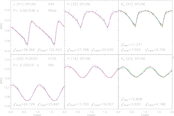
Figure 6. Top: light curve for the RRab variable V44. The red line shows the spline fit, while the blue line the PLOESS fit and the green line the template fit. The vertical error bars display the intrinsic photometric error. The name and the period of the variable are labelled in the top-left panel. In the top-left corner of each panel, the fitting model (spline, PLOESS) that was selected as the best one, is labelled. Bottom: same as the top, but for the RRc variable V105.
Download figure:
Standard image High-resolution image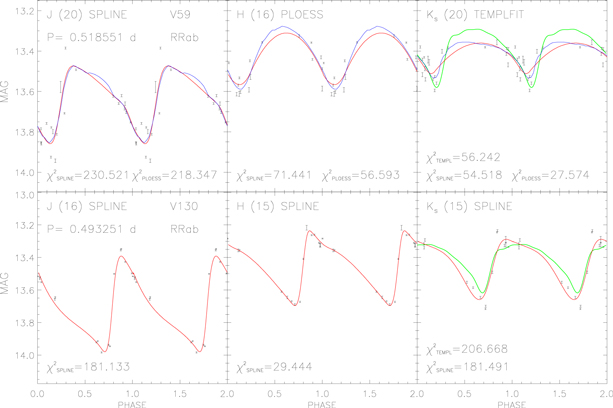
Figure 7. Top: same as the top in Figure 6, but for the RRab variable V59. Bottom: same as the top, but for the RRab variable V130.
Download figure:
Standard image High-resolution imageOnce the fits to the light curves were performed (spline, PLOESS, template), we derived the mean magnitudes, photometric amplitudes, and their uncertainties. Note that the mean magnitudes were derived by converting magnitudes to intensity, in arbitrary units, then averaging and re-converting to magnitudes. For the RRLs for which either the phase coverage is not optimal or the light curve is too noisy, the final value of the mean magnitude was estimated as the median of the magnitudes converted to intensity over the individual phase points. Photometric amplitudes were derived by the difference between the maximum and minimum of the fit of the light curve, whereas the mean magnitude was derived by either the spline or the PLOESS fit. The uncertainty on the photometric amplitudes were estimated summing in quadrature the median photometric error of the phase points around the minimum and the maximum of the light curve plus the standard deviation of the same phase points around the fit of the light curve. The final value was weighted with the number of phase points around minimum and maximum phases. The error on the amplitudes, for the few light curves with no phase points either across minimum or maximum phase, were estimated by summing in quadrature the difference between the maximum/minimum of the fit and the faintest/brightest phase point. Note that we do not provide the photometric amplitude from template fit, since this parameter is an input in this approach. The mean magnitudes, the amplitudes, and their errors from the fits of the light curves are listed in Table 2. We also provide new optical mean magnitudes and amplitudes in Table 3. Figures 6 and 7 also display a pseudo-χ2 statistics for each fit:
Taking account of the smallness of the photometric errors (errobs), the derived χ2 are low (see Figures 6 and 7). This is further evidence of the goodness of fit of the light curves. Note that, on the basis of both a visual inspection of the light curves, and the comparison of the uncertainties on the means magnitude and amplitudes, we selected for each RRL the most accurate fit among spline, PLOESS and template. Note that the fits that we selected are not always those with the smallest χ2.
Figures 8 and 9 show the difference in mean magnitude between the three different methods adopted to fit the light curves. Spline and PLOESS provide mean magnitudes that are very similar, indeed the difference and the standard deviations are vanishing (ΔJ = 0.000 ± 0.006, ΔH = 0.000 ± 0.006, ΔKs = 0.000 ± 0.004 mag). However, photometric amplitudes display more significant differences between spline and PLOESS fits: they range from a few thousandths for low-amplitude RRc variables to one or two tenths of a magnitude for short-period, large-amplitude RRab variables. The difference for the latter group is mainly caused by the fact that the PLOESS fits better represent the ripple across the minimum light phases than the spline.
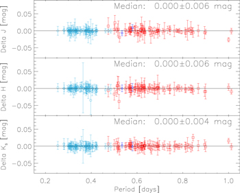
Figure 8. Top: difference between the mean J-band magnitudes estimated using the spline and the PLOESS fit as a function of the pulsation period. Light blue circles and red squares mark RRc (first overtone) and RRab (fundamental) variables. Dark blue diamonds mark variables of uncertain type. Middle: same as the top, but for the H-band. Bottom: same as the top, but for the Ks-band.
Download figure:
Standard image High-resolution image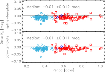
Figure 9. Top: difference between the mean Ks-band magnitudes derived using the spline and the template fit as a function of the pulsation period. Symbols are the same as in Figure 8. Bottom: same as the top, but the difference is between the PLOESS and the template fit.
Download figure:
Standard image High-resolution imageWe note that template fits have at least three disadvantages. One is the aforementioned sensitivity to the period: an error of 10−5 days or larger may lead to a wrong phasing of the light curve, even with accurate epochs of maximum. Moreover the light curve template of RRc stars has a fixed amplitude because it is based only on four of them and it was not possible to establish a relation between optical and NIR amplitudes. Finally, as shown in Figure 9, the mean magnitudes obtained from the template fits are ∼0.01 mag fainter than those obtained with spline or PLOESS fitting. Most of the time, this difference is caused by the deeper minima of the template fits with respect to the other fitting functions.
3.4. Comparison of NIR Mean Magnitudes
We compare the mean magnitudes that we obtain with those of Longmore et al. (1990), Sollima et al. (2006a), and Navarrete et al. (2017). To make the comparison in the same photometric system (2MASS), we have adopted the transformations of Carpenter (2001) to convert the AAO mean magnitudes of Longmore et al. (1990). Since these transformations need J–KAAO as an input, but the J-band magnitude is not provided by Longmore et al. (1990), we have adopted J–KAAO = 0.25 mag for all RRLs. This is an approximate mean of the J–Ks colors of RRLs. We point out that a shift of 0.05 mag in J–KAAO means a change of 0.01 mag in the output Ks-band magnitude. The J–Ks colors of RRLs range from 0.15 and 0.40 mag, therefore, the uncertainty on the adopted mean J–KAAO color is at most 0.15 mag. This means that the uncertainty on the transformed Ks-band magnitude is 0.03 mag. This amount is around half of the mean offset (see Figure 10), thus supporting the idea to set the same J–KAAO for all RRLs, so it is fine to set the same J–KAAO for all RRLs. Sollima et al. (2004) provides the offset of their photometry—the same as used in Sollima et al. (2006a)—with the 2MASS photometric system: ΔJ = 0.00 ± 0.10 mag and ΔKs = −0.04 ± 0.10 mag. We adopt these corrections to derive the offset from our mean magnitudes. The VISTA-system mean magnitudes of Navarrete et al. (2017) were transformed adopting the equations provided by CASU (http://casu.ast.cam.ac.uk/surveys-projects/vista/technical/photometric-properties; González-Fernández et al. 2018).
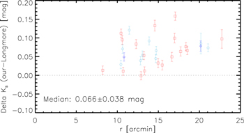
Figure 10. Difference between our final Ks-band mean magnitudes and those derived by Longmore et al. (1990) as a function of the radial distance from the center of the cluster. The label depicts the median and the standard deviation of the sample. The vertical bars display the sum in quadrature of the uncertainties on mean magnitudes of the two data sets. Symbols are the same as in Figure 8.
Download figure:
Standard image High-resolution imageThe systematic offset between the photometry of Longmore et al. (1990) and ours is 0.067 ± 0.036 mag. We point out that their estimate of the distance modulus (13.61 mag) is among the smallest in the literature. If we assume that our photometry is more accurate and correct their distance modulus by the quoted offset, we obtain 13.68 mag, which is much closer to the bulk of other distance modulus estimates, especially those derived from RRLs (see Section 6). The work of Longmore et al. (1990) was only focused—as is clear in Figure 10—on RRLs far from the center of the cluster. Therefore, it is unlikely that the offset is due to blended sources in their photometry. A more plausible explanation is that the standard stars for the calibration of the AAO (Allen & Cragg 1983) have K-band magnitudes all between 1.5 and 6.0 mag, that are much brighter than any RRL in ω Cen. Moreover, only four of these stars were retrieved in the 2MASS catalog by Carpenter (2001) to derive the AAO–2MASS transformations. Ten more stars from Elias et al. (1983) were used but these were not considered to be primary standards. We conclude that the offset that we found is most likely due to a combination of an inaccurate calibration—even if it was the best possible one—and to a non-precise and, possibly, inaccurate transformation between the AAO and 2MASS system.
The comparison with Sollima et al. (2006a) gives small median offsets both in the J (∼0.02 mag) and in the Ks band (∼0.01 mag). However, the dispersion of the magnitude offsets is large (∼0.10 and ∼0.08 mag in J and Ks band, respectively) compared to the median (see Figure 11). We can safely assume the overall offset to be null in both bands. The large sigma is most likely due to the paucity of phase points that were collected for that program, as it was not primarily conceived to obtain RRLs time-series data.
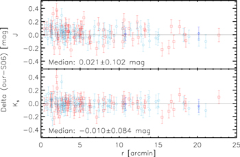
Figure 11. Top: difference between our final J-band mean magnitudes and those derived by Sollima et al. (2006a) as a function of the radial distance from the center of the cluster. The label depicts the median and the standard deviation of the sample. The vertical bars display the sum in quadrature of the uncertainties on mean magnitudes of the two data sets; symbols are the same as in Figure 8. Bottom: same as the top, but for the Ks-band mean magnitudes.
Download figure:
Standard image High-resolution imageFigure 12 shows the comparison of our mean magnitudes with those of Navarrete et al. (2017). The median offset is ∼0.03 mag in both J and Ks. However, we note that, in the J band, there is a trend with distance in the innermost region of the cluster: the closer the star to the cluster center, the brighter the mean magnitudes of Navarrete et al. (2017) compared to ours. This is probably due to better angular resolution of blended sources in our photometry. This hypothesis is also supported by the difference in the pixel scales of FourStar (0.16 arcsec/pixel) and VIRCAM (0.34 arcsec/pixel). Note that the rise in the offset of the Ks magnitudes at distances from the center larger than 20 arcmin is only apparent and no firm conclusion can be derived, due to a paucity of RRLs in these cluster regions.
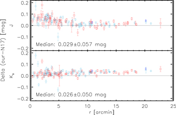
Figure 12. Top: difference between our final J-band mean magnitudes and those derived by Navarrete et al. (2017) as a function of the radial distance from the center of the cluster. The label depicts the median and the standard deviation of the sample. The vertical bars display the sum in quadrature of the uncertainties on mean magnitudes of the two data sets; symbols are the same as in Figure 8. Bottom: same as the top, but for the Ks-band mean magnitudes.
Download figure:
Standard image High-resolution image4. NIR Pulsation Properties of RR Lyrae Variables
4.1. RRL Instability Strip in NIR and in Optical–NIR CMDs
Figure 13 shows the entire set of candidate cluster RRLs in ω Cen in the J, J–H and in the J, J–Ks CMDs. The properties of field variables and misclassified variables are discussed in more detail in the Appendix. In this context we note only that candidate field variables are located at radial distances larger than 9 arcmin from the cluster center.
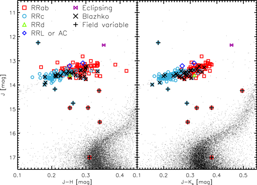
Figure 13. Left: NIR (J vs. J–H) CMD of ω Cen (black dots, LCO13 data set). Symbols are the same as in Figure 8. The candidate RRd variable V142 is marked with a green triangle, the eclipsing binary V179 is marked with a purple bowtie, while the black crosses display candidate Blazhko variables. Field variables are marked with a black plus. Right: same as the left, but for the J vs. J–Ks CMD.
Download figure:
Standard image High-resolution imageThe typical uncertainties of the mean NIR magnitudes are at most of the order of a few hundredths of a magnitude. This indicates that the range in magnitude covered by the candidate cluster RRLs is intrinsic.
To further improve the analysis of the candidate cluster RRLs inside the instability strip, we adopted an optical–NIR CMD (Figure 14). The color sensitivity increases by almost a factor of four (0.2–0.3 versus 1.1 mag) when moving from NIR to optical–NIR CMDs. The increased sensitivity in effective temperature provides the opportunity to trace the topology of the instability strip. Indeed, the first overtone variables are systematically bluer/hotter than fundamental pulsators. They overlap in a region called the "OR" region (van Albada & Baker 1973; Bono & Stellingwerf 1993; Bono et al. 1997; Caputo 1998), i.e., the region in which they can pulsate either in the fundamental or in the first overtone mode. The predicted topology is further supported by the new mixed-mode candidate identified by Braga et al. (2016) even if the actual pulsation mode distribution in the OR region is related to the so-called "hysteresis mechanism" (van Albada & Baker 1973; Bono et al. 1995, 1997).
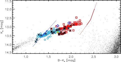
Figure 14. Close-up of the RRL instability strip of the optical–NIR (Ks vs. B–Ks) CMD of ω Cen. The optical photometry for both static and variable stars comes from Braga et al. (2016), while the NIR is based on the LCO13 data set. The almost vertical blue and red lines display the predicted first overtone blue edge and the fundamental red edge according to Marconi et al. (2015), at Z = 0.0006 ([Fe/H] = −1.84; α-enhanced mixture).
Download figure:
Standard image High-resolution imageThe candidate cluster variables display a narrow distribution in magnitude and color. The increased sensitivity of the optical–NIR magnitudes allows us to investigate in more detail the location of candidate Blazhko RRLs. Data plotted in Figure 14 display that they are mainly concentrated in the transition between RRc and RRab, as recently suggested by Braga et al. (2016). This finding supports previous results by Jurcsik et al. (2011) concerning Blazhko RRLs in the Galactic globular M5. Furthermore, it is suggesting that the iron content, in the metallicity range covered by RRLs in ω Cen, is playing a marginal role in the transition from RRc to RRab. Moreover, there is mounting evidence that they cover the entire range of colors typical of RRc variables. This empirical evidence is consistent with recent investigations of Blazhko variables in the Galactic Bulge (Prudil & Skarka 2017). Interestingly, at ∼0.7 days, the NIR/optical photometric amplitude ratios display an increase compared to short-period RRLs (see Section 4.2). These findings need to be cautiously treated. The referee found, using optical photometry by Kaluzny et al. (2004), that the variable V38 (P = 0.779 days) is indeed a low-amplitude candidate Blazhko RRL. Moreover, she also suggested that the detection of Blazhko RRLs in the long-period tail is very difficult because the amplitude modulation steadily decreases. In passing we note that similar evidence was recently brought forward by Jurcsik et al. (2018) using Galactic bulge RRab variables. These are very interesting findings worth being investigated in globulars with sizable samples of RRLs, since the age and the chemical composition of their progenitors is well defined.
The same figure also shows reasonable agreement between the predicted first overtone blue edge (blue solid line) plus fundamental red edge (red solid line) provided by Marconi et al. (2015) and observations. However, the predicted edges are slightly redder compared to optical–NIR observations. The difference is of the order of Δ(B–Ks) ∼ 0.10–0.15 mag, meaning a difference in effective temperature of the order of ∼250 K. In the comparison between theory and observation we must take account of several basic assumptions. The predicted edges were estimated assuming a fixed metal content, Z = 0.0006 and an α-enhanced mixture, which means [Fe/H] = −1.84 (similar to the peak in metallicity found by Johnson & Pilachowski 2010). Furthermore, the analytical relations used to estimate the position of the edges are based on pulsation models computed with a resolution in effective temperature of ± 50 K. In a forthcoming investigation we also plan to study the impact that stellar atmosphere models have in transforming pulsation predictions into the observational plane (Marconi et al. 2015). On the observational side, we are assuming the same cluster reddening for the entire sample of RRLs, but there is evidence of reddening variation (Δ(B–V) ∼ 0.03 mag) across the body of the cluster (Calamida et al. 2005).
It is worth mentioning that candidate RRLs are far from being uniformly distributed in color and magnitude across the instability strip. Castellani et al. (2007), using a photometric catalog based both on space (HST) and on ground-based wide-field images, found that the luminosity function either in magnitude or in color of HB stars has a clumpy distribution. This means that the number of hot HB stars per magnitude interval is not uniform, since they display well-defined peaks and gaps. The same outcome applies to the instability strip; indeed, the width in color of the instability strip in the K, B–K CMD is roughly one magnitude (B–K ∼ 1.2–2.2 mag). The number of RRLs located in the bluer region (B–K < 1.45 mag, 40 objects) is higher than in the redder region (B–K > 1.95 mag, 26 objects). Note that this analysis can be barely performed in the V, B–V CMD, since the width in color of the instability strip is only 0.4 mag (B–V ∼ 0.2–0.6 mag). The current photometric accuracy and the homogenous estimates of both optical and NIR mean magnitudes bring forward the occurrence of multiple sequences not only among RRab variables, but also among RRc variables. This evidence suggests that the metallicity distribution of RRLs in ω Cen is indeed multi-modal. Unfortunately, the accuracy of the current spectroscopic and photometric metallicity estimates does not allow us to constrain, on a quantitative basis, the magnitude–metallicity variation.
4.2. Bailey Diagram and Photometric Amplitude Ratios
The amplitudes of long-period (P ≳ 0.7 days) RRab show an almost flat distribution in the NIR Bailey diagrams (Figure 15). This is different from the optical Bailey diagrams, where the amplitudes steadily decrease toward longer periods (Braga et al. 2016). To better understand the different behavior of optical and NIR amplitudes, we have calculated the NIR-over-optical and the H, Ks-over-J-band light-amplitude ratios of the RRLs in ω Cen and we have divided the candidate RRLs into three groups: RRc, short-period RRab (P ≲ 0.7 days), and long-period RRab (P ≳ 0.7 days). The results are shown in Figures 16–18.
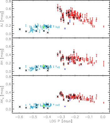
Figure 15. Top: J-band photometric amplitude vs. logarithmic period (Bailey diagram) for ω Cen RRLs. Uncertainties on the amplitudes are shown as vertical error bars. The symbols and the color coding is the same as in Figure 13. Middle: same as the top, but for H-band amplitudes. Bottom: same as the top, but for Ks-band amplitudes.
Download figure:
Standard image High-resolution image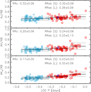
Figure 16. Top: NIR/optical (AJ/AB) amplitude ratios as a function of the logarithmic period. The median and the standard deviation of the RRc sample, of the short-period ( ) RRab, and of the long-period RRab (
 ) are plotted as solid and dotted horizontal lines (see also labelled values). Middle: same as the top, but for AH/AB amplitude ratios. Bottom: same as the top, but for AKs/AB amplitude ratios.
Download figure:
Standard image High-resolution image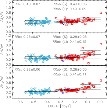
Figure 17. Same as Figure 16, but the amplitude ratios are among NIR bands and the visual bands: AJ/AV (top), AH/AV (middle), and AKs/AV (bottom).
Download figure:
Standard image High-resolution image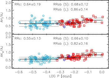
Figure 18. Same as Figure 16, but for the NIR amplitude ratio AH/AJ (top) and AKs/AJ (bottom).
Download figure:
Standard image High-resolution imageIn Table 4, we show the median light-amplitude ratios of the RRc, short-period RRab, and long-period RRab. Note that we use the median instead of the mean and that the outliers are ruled out, because these ratios will be crucial to derive new light-curve templates and one must be as accurate as possible to avoid systematic errors.
Table 4. Mean Amplitude Ratios of RRc, Short-period RRab, and Long-period RRab Stars of ω Cen RRLs
| RRc | RRab (short) | RRab (long) | ||||
|---|---|---|---|---|---|---|
| mean | σ | mean | σ | mean | σ | |
| AJ/AB | 0.316 | 0.062 | 0.350 | 0.063 | 0.394 | 0.097 |
| AH/AB | 0.198 | 0.058 | 0.237 | 0.055 | 0.331 | 0.161 |
| AKs/AB | 0.172 | 0.051 | 0.233 | 0.034 | 0.323 | 0.126 |
| AJ/AV | 0.396 | 0.066 | 0.429 | 0.057 | 0.488 | 0.106 |
| AH/AV | 0.252 | 0.071 | 0.286 | 0.055 | 0.414 | 0.202 |
| AKs/AV | 0.221 | 0.061 | 0.280 | 0.028 | 0.407 | 0.169 |
| AH/AJ | 0.647 | 0.183 | 0.676 | 0.118 | 0.861 | 0.238 |
| AKs/AJ | 0.551 | 0.128 | 0.658 | 0.093 | 0.822 | 0.229 |
Download table as: ASCIITypeset image
We found that the median of the amplitude ratios of RRc is systematically smaller than that of the short-period RRab, whatever the combination of NIR-to-optical photometric bands. Note that this behavior is more and more evident moving from J (mild increase of amplitude ratios with period) to Ks. As a consequence, the increase with period is also seen in the J-over-Ks amplitude ratio. This behavior is different from what was found for the optical-to-optical amplitude ratios (constant over all the periods and pulsation modes; Braga et al. 2016).
This is the first time that a clear difference, based on a large statistical sample, between the NIR-over-optical amplitude ratios of RRab and RRc is found. An analogous result was obtained by Inno et al. (2015), who found a dichotomy in the NIR-over-optical amplitude ratios of Cepheids in the Magellanic Clouds (MCs) and the Milky Way. They found that short-period (P < 20 days) Cepheids have amplitude ratios that are smaller than long-period Cepheids. A detailed study of the amplitude ratios of RRLs in several GGCs was done by Kunder et al. (2013), but they used only optical data and found no statistically relevant dichotomy in the amplitude ratios of RRab and RRc.
We have also found that RRab variables, for periods longer than ∼0.7 days, display a well defined increse in the optical/NIR amplitude ratios. In a recent investigation, Jurcsik et al. (2018) found evidence of a linear increase in the AK over AI amplitude ratio of Galactic Bulge RRab variables, when moving from short to long periods. It is not clear whether the difference in the two behaviors is either intrinsic (e.g., due to the metallicity distribution) or the consequence of a selection bias.
We have also found that, at periods longer than ∼0.7 days, the ratios with AH and AKs in the denominator are no longer constant and increase more or less linearly with increasing  . This trend is absolutely unique and has never before been found even for pulsating variables of other types (SX Phe, Classical and Type II Cepheids).
5. Period–Luminosity Relations
The current NIR data set provided an opportunity to investigate in detail the NIR PL relations.
Spread and slope of the PL relations. Data plotted in Figure 19 show that the standard deviations of RRab (red squares, left panel) RRc (light blue circles, left panel) and Global (right panels)26 variables remain almost constant (0.04–0.05 mag) when moving from the J to the Ks band. This is a significant advantage when compared with the standard deviations in the I-band (Global, 0.06–0.08 mag) of the same variables (Braga et al. 2016). The same outcome applies to the slopes of the PL relations; indeed they increase for the RRc from −2.105 (J) to −2.531 (Ks), for the RRab from −2.318 (J) to −2.621 (Ks) and for the Global sample from −1.884 (J) to −2.380 (Ks). The improvement is even more relevant when compared with the slopes for the I-band (RRc, −1.624; RRab, −1.955; Global, −1.335).
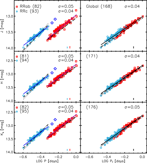
Figure 19. Top left: J-band PL relations for fundamental (RRab) and first overtone (RRc) RRLs in ω Cen. The black solid lines display the linear fit for RRc and RRab. The number of RRab and RRc variables that passed the sigma clipping (2.8σ) is labelled. The error bars in the bottom-right corner display the standard deviations (see also labelled values). The black dotted/dashed lines display the theoretical PL relations for RRc and RRab variables according to Marconi et al. (2015), obtained with/without including the solar metallicity models in the derivation of the theoretical PLs. The predicted relations were plotted assuming a true distance modulus of 13.71 mag (Braga et al. 2016) and a mean reddening of 0.11 mag (Thompson et al. 2001; Lub et al. 2002). Top right: same as the left, but for the Global sample, i.e., the periods of RRc variables were fundamentalized:  =
=  . Middle: same as the top, but for the H-band PL relation. Bottom: same as the top, but for the Ks-band PL relation.
Download figure:
Standard image High-resolution imageMetallicity dependence. We performed a linear fit over the entire data set and the resulting coefficients are listed in Table 5. The errors on the mean magnitudes are on average of the order of a few hundredths of a magnitude (see Table 5). This indicates that the dispersion along the PL relations and the errors on the slopes are dominated by an intrinsic feature. In particular, several variables are intrinsically either brighter or fainter than the linear fit. This suggests that they are either more metal-poor or more metal-rich than the bulk of RRL variables. This further supports recent findings concerning the metallicity dependence of the RRL PL relations based on theoretical (Marconi et al. 2015) and on semi-empirical (Neeley et al. 2017) arguments.
Table 5.
Coefficients of the Observed PL Relations of RRab, RRc and RRab Plus Fundamentalized RRc Stars of ω Cen of the Form X = a + 
| RRc | RRab | Global | |||||||
|---|---|---|---|---|---|---|---|---|---|
| a | b | σ | a | b | σ | a | b | σ | |
| mag | mag | mag | mag | mag | mag | mag | mag | mag | |
| J | 12.666 | −2.105 | 0.036 | 12.963 | −2.318 | 0.050 | 13.018 | −1.884 | 0.043 |
| ±0.030 | ±0.067 | ⋯ | ±0.014 | ±0.073 | ⋯ | ±0.010 | ±0.034 | ⋯ | |
| H | 12.314 | −2.403 | 0.040 | 12.643 | −2.520 | 0.046 | 12.686 | −2.224 | 0.043 |
| ±0.034 | ±0.075 | ⋯ | ±0.014 | ±0.069 | ⋯ | ±0.009 | ±0.034 | ⋯ | |
| Ks | 12.244 | −2.531 | 0.042 | 12.591 | −2.621 | 0.048 | 12.625 | −2.380 | 0.046 |
| ±0.035 | ±0.076 | ⋯ | ±0.014 | ±0.070 | ⋯ | ±0.010 | ±0.036 | ⋯ | |
Download table as: ASCIITypeset image
The peak of the metallicity distribution in ω Cen is [Fe/H] ≈ −1.8 (Johnson & Pilachowski 2010). To provide more quantitative constraints, we performed a detailed comparison with predicted NIR PL relations recently provided by Marconi et al. (2015). In this investigation the authors provided NIR PL relations that either neglect (metal-independent) or take account of the metallicity dependence. The key advantage of the quoted predictions is that they cover a broad range in stellar masses, luminosity levels and chemical compositions. In particular, they adopted an α-enhanced chemical composition, a constant helium-to-metal enrichment ratio and seven different metal abundances ranging from Z = 0.0001 to Z = 0.0198. This means that the predictions cover more than two dex in iron abundance. The dotted lines plotted in Figure 19 display the metal-independent PL relation, and the agreement for both RRab, RRc, and Global variables is quite good, if we take account of the significantly different metallicity distributions covered by theory and observations. Indeed, once predicted metal-independent PL relations are restricted to models more metal-poor than solar (Z ≤ 0.008), the predicted relations display zero-points and slopes that agree better with the observed ones (see dashed lines on the same figure).
The above circumstantial evidence indicates that NIR PL relations depend on metallicity. To further investigate this effect we computed new empirical period–luminosity–metallicity (PLZ) relations using three different sets of iron abundances: (1) spectroscopic estimates for 74 RRLs provided by Sollima et al. (2006a); (2) photometric estimates based on Ca, b, y photometry provided by Rey et al. (2000) for 131 RRLs; (3) photometric estimates obtained by Braga et al. (2016) by inverting the I-band PLZ relation for 160 RRLs.
The coefficients of the surface fits and their uncertainties are listed in Table 6, while Figure 20 shows the NIR PLZ relations in 3D plots. There is evidence that the spread in magnitude is, at fixed period, dominated by the spread in metal abundances. The metallicity estimates are affected, on average, by uncertainties of the order of 0.2 dex. The difference among the three different sets of metal abundances is caused by the sample size; indeed the metallicity estimates by Braga et al. (2016) are more than a factor of two larger than the spectroscopic sample of Sollima et al. (2006a). The sample size can play a crucial role in constraining the spread in metallicity. Short-period RRc variables are marginally present in the Rey et al. (2000) sample, but they appear in Sollima et al. (2006a) and in Braga et al. (2016). The current data suggest that they fix the metal-poor tail of the sample.
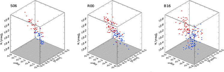
Figure 20. Left: Ks-band period–luminosity–metallicity relation for RRLs in ω Cen. The photometric metallicity ([Fe/H]) estimates come from Sollima et al. (2006a). The symbols and the color coding are the same as in Figure 13. Middle: same as the left, but spectroscopic metal abundances according to Rey et al. (2000). Right: same as the left, but photometric metallicity estimates according to (Braga et al. 2016, Table 10, fifth column).
Download figure:
Standard image High-resolution imageTable 6.
Coefficients of the Observed PLZ Relations of RRab, RRc and RRab Plus Fundamentalized RRc Stars of ω Cen of the Form X = a +  + c [Fe/H]
| RRc | RRab | Global | ||||||||||
|---|---|---|---|---|---|---|---|---|---|---|---|---|
| a | b | c | σ | a | b | c | σ | a | b | c | σ | |
| mag | mag | mag | mag | mag | mag | mag | mag | mag | mag | mag | mag | |
| [Fe/H] from Rey et al. (2000) | ||||||||||||
| Free parameters | ||||||||||||
| J | 12.711 | −2.112 | 0.026 | 0.034 | 13.093 | −2.284 | 0.077 | 0.038 | 13.124 | −1.873 | 0.061 | 0.046 |
| ±0.058 | ±0.092 | ±0.018 | ⋯ | ±0.035 | ±0.071 | ±0.018 | ⋯ | ±0.032 | ±0.052 | ±0.016 | ⋯ | |
| H | 12.374 | −2.394 | 0.034 | 0.036 | 12.780 | −2.502 | 0.081 | 0.034 | 12.779 | −2.225 | 0.056 | 0.040 |
| ±0.061 | ±0.097 | ±0.019 | ⋯ | ±0.030 | ±0.063 | ±0.015 | ⋯ | ±0.028 | ±0.045 | ±0.014 | ⋯ | |
| Ks | 12.304 | −2.531 | 0.033 | 0.038 | 12.753 | −2.601 | 0.096 | 0.038 | 12.725 | −2.386 | 0.062 | 0.045 |
| ±0.065 | ±0.103 | ±0.021 | ⋯ | ±0.033 | ±0.069 | ±0.017 | ⋯ | ±0.030 | ±0.050 | ±0.015 | ⋯ | |
| Fixed slopea | ||||||||||||
| J | 12.522 | −2.458 | −0.002 | 0.033 | 13.203 | −1.964 | 0.108 | 0.044 | 13.120 | −1.883 | 0.060 | 0.046 |
| ±0.025 | ±0.089 | ±0.016 | ⋯ | ±0.031 | ±0.039 | ±0.019 | ⋯ | ±0.023 | ±0.032 | ±0.014 | ⋯ | |
| H | 12.193 | −2.716 | 0.006 | 0.039 | 12.852 | −2.225 | 0.092 | 0.039 | 12.783 | −2.214 | 0.058 | 0.040 |
| ±0.029 | ±0.049 | ±0.019 | ⋯ | ±0.028 | ±0.023 | ±0.017 | ⋯ | ±0.020 | ±0.019 | ±0.013 | ⋯ | |
| Ks | 12.186 | −2.740 | 0.016 | 0.039 | 12.850 | −2.260 | 0.116 | 0.043 | 12.782 | −2.249 | 0.077 | 0.046 |
| ±0.030 | ±0.048 | ±0.019 | ⋯ | ±0.031 | ±0.022 | ±0.018 | ⋯ | ±0.023 | ±0.018 | ±0.014 | ⋯ | |
| [Fe/H] from Sollima et al. (2006a) | ||||||||||||
| Free parameters | ||||||||||||
| J | 12.826 | −1.935 | 0.056 | 0.028 | 13.284 | −2.013 | 0.162 | 0.027 | 13.286 | −1.773 | 0.146 | 0.031 |
| ±0.094 | ±0.102 | ±0.040 | ⋯ | ±0.046 | ±0.076 | ±0.022 | ⋯ | ±0.035 | ±0.042 | ±0.019 | ⋯ | |
| H | 12.392 | −2.304 | 0.026 | 0.033 | 12.908 | −2.249 | 0.135 | 0.033 | 12.916 | −2.163 | 0.133 | 0.032 |
| ±0.110 | ±0.118 | ±0.047 | ⋯ | ±0.050 | ±0.091 | ±0.025 | ⋯ | ±0.037 | ±0.043 | ±0.020 | ⋯ | |
| Ks | 12.367 | −2.442 | 0.057 | 0.035 | 12.876 | −2.367 | 0.148 | 0.025 | 12.894 | −2.281 | 0.152 | 0.029 |
| ±0.116 | ±0.126 | ±0.049 | ⋯ | ±0.038 | ±0.070 | ±0.019 | ⋯ | ±0.033 | ±0.039 | ±0.018 | ⋯ | |
| Fixed slopea | ||||||||||||
| J | 12.429 | −2.458 | −0.039 | 0.040 | 13.303 | −1.964 | 0.180 | 0.063 | 13.272 | −1.883 | 0.159 | 0.055 |
| ±0.087 | ±0.089 | ±0.051 | ⋯ | ±0.070 | ±0.039 | ±0.041 | ⋯ | ±0.054 | ±0.032 | ±0.031 | ⋯ | |
| H | 12.123 | −2.716 | −0.024 | 0.038 | 12.916 | −2.225 | 0.137 | 0.032 | 12.898 | −2.214 | 0.130 | 0.032 |
| ±0.091 | ±0.049 | ±0.053 | ⋯ | ±0.038 | ±0.023 | ±0.023 | ⋯ | ±0.034 | ±0.019 | ±0.020 | ⋯ | |
| Ks | 12.169 | −2.740 | 0.019 | 0.037 | 12.915 | −2.260 | 0.160 | 0.026 | 12.905 | −2.249 | 0.154 | 0.029 |
| ±0.085 | ±0.048 | ±0.049 | ⋯ | ±0.029 | ±0.022 | ±0.018 | ⋯ | ±0.030 | ±0.018 | ±0.017 | ⋯ | |
| [Fe/H] from Braga et al. (2016) | ||||||||||||
| Free parameters | ||||||||||||
| J | 12.755 | −2.178 | 0.068 | 0.031 | 13.184 | −2.152 | 0.110 | 0.034 | 13.139 | −1.886 | 0.068 | 0.037 |
| ±0.029 | ±0.059 | ±0.010 | ⋯ | ±0.035 | ±0.061 | ±0.017 | ⋯ | ±0.019 | ±0.031 | ±0.010 | ⋯ | |
| H | 12.383 | −2.470 | 0.054 | 0.032 | 12.856 | −2.412 | 0.109 | 0.036 | 12.795 | −2.265 | 0.066 | 0.037 |
| ±0.030 | ±0.061 | ±0.010 | ⋯ | ±0.035 | ±0.062 | ±0.017 | ⋯ | ±0.019 | ±0.031 | ±0.009 | ⋯ | |
| Ks | 12.301 | −2.672 | 0.067 | 0.032 | 12.846 | −2.474 | 0.130 | 0.032 | 12.753 | −2.401 | 0.075 | 0.039 |
| ±0.031 | ±0.063 | ±0.010 | ⋯ | ±0.035 | ±0.058 | ±0.017 | ⋯ | ±0.020 | ±0.032 | ±0.010 | ⋯ | |
| Fixed slopea | ||||||||||||
| J | 12.642 | −2.458 | 0.075 | 0.036 | 13.249 | −1.964 | 0.127 | 0.035 | 13.173 | −1.883 | 0.086 | 0.042 |
| ±0.020 | ±0.089 | ±0.011 | ⋯ | ±0.029 | ±0.039 | ±0.016 | ⋯ | ±0.019 | ±0.032 | ±0.010 | ⋯ | |
| H | 12.288 | −2.716 | 0.063 | 0.032 | 12.917 | −2.225 | 0.124 | 0.038 | 12.806 | −2.214 | 0.065 | 0.038 |
| ±0.018 | ±0.049 | ±0.010 | ⋯ | ±0.031 | ±0.023 | ±0.017 | ⋯ | ±0.018 | ±0.019 | ±0.010 | ⋯ | |
| Ks | 12.274 | −2.740 | 0.069 | 0.032 | 12.916 | −2.260 | 0.149 | 0.038 | 12.793 | −2.249 | 0.076 | 0.044 |
| ±0.018 | ±0.048 | ±0.010 | ⋯ | ±0.032 | ±0.022 | ±0.018 | ⋯ | ±0.020 | ±0.018 | ±0.011 | ⋯ | |
Note.
aWe have fixed b at the value of the slope of the predicted PLZ.Download table as: ASCIITypeset image
To show even more clearly the dependence on metallicity of the PL relations, we also display, in Figure 21, the residuals of the Ks-band mean magnitudes with respect to the PLZ at fixed iron abundance ([Fe/H] −1.8 dex). This metal abundance was selected because it is the peak of the RRL metallicity distribution (Braga et al. 2016). The residuals display a clear trend in spite of the large dispersion. This means that the lack of a metallicity term in the PL relations leads to magnitudes that are systematically brighter/fainter for metal-poor/metal-rich RRLs.
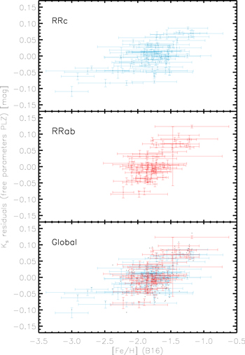
Figure 21. Top: residuals of the Ks-band mean magnitudes of RRc stars minus the empirical PLZ—derived by leaving free all the parameters and using metallicities by Braga et al. (2016)—at fixed [Fe/H] = −1.8 dex, vs. iron abundance. Middle: same as the top, but for RRab stars. Bottom: same as the top, but for the Global sample.
Download figure:
Standard image High-resolution imageTo further quantify the spread in metal abundance of ω Cen RRLs, Figure 22 shows the Ks-band PL relation together with predicted PLZ relations at fixed metal abundance (dashed lines). The comparison between theory and observations indicates that the RRLs span more than one dex in metal abundance, indeed they range from [Fe/H] ≈ −2.3 to ≈−1.3. To further validate the quoted trend we decided to perform a linear fit to the mean NIR magnitudes using the predicted slope for the period dependence and at fixed metal content ([Fe/H] = −1.8).
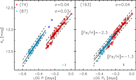
Figure 22. Left: Ks-band PL relation for RRab and RRc in ω Cen. The black dashed lines display the predicted PLZ relations by Marconi et al. (2015) at two fixed metal abundances: [Fe/H] = −1.3 (fainter) and [Fe/H] = −2.3 (brighter). Theory was plotted assuming a true distance modulus of 13.71 mag and a mean cluster reddening of 0.11 mag (Thompson et al. 2001; Lub et al. 2002). The black solid lines display the surface fit to the data—the coefficients are listed in Table 6—by assuming a fixed metal abundance ([Fe/H] = −1.8) and the slopes predicted from theory. The number of variables adopted in the fit and the standard deviations from the PLZ relations are also labelled. The error bars in the bottom-right corner display the standard deviations (see also labelled values). Right: same as the left, but for the Global (RRab+RRc) sample. The black dotted–dashed line shows the PLZ relation derived by Navarrete et al. (2017) assuming a metal content of [Fe/H] = −1.8.
Download figure:
Standard image High-resolution imageThe black solid lines plotted in the left panel of this figure show very good agreement between theory and observations for both RRc and RRab variables over the entire period range. The outcome is the same for the fundamentalized PLZ relation (black solid line in the right panel) plotted in the right panel of the same figure. This panel also shows the comparison with the empirical PLZ relation recently derived by Navarrete et al. (2017). The agreement is also reasonable, but it covers the upper envelope of the observed distribution. This difference is easily explained by the difference between our mean magnitudes and those of Navarrete et al. (2017), already addressed in Section 3.4. The referee suggested to double check the impact of the individual sigma clipping applied to estimate the PLZ relations. We computed a new set of PLZ relations using the same sigma clipping that we adopted for the metal-independent PL relations. We found that the coefficients of the PLZ relations are, within the errors, minimally affected by the different sigma clipping that we applied.
We also note, in Table 6, that the best agreement for the metallicity coefficients of the PLZ relations is found for the RRab and the Global sample using the iron abundances from Sollima et al. (2006a). The metallicity coefficients of RRc PLZ relations are almost null when we adopt either the Rey et al. (2000) or the Sollima et al. (2006a) iron abundances. On the other hand, the agreement with the predicted PLZs (Marconi et al. 2015) is good when using abundances provided by Braga et al. (2016) and the dispersion among RRc, RRab, and Global samples is also smaller. Finally, the dispersion of the data around the PLZ is only marginally smaller (<0.01 mag) than the dispersion around the PL relations (see Figures 19 and 22). This further supports the uncertainties affecting the current spectroscopic estimates.
Figures 19 and 22 also show the position of the two variables (V68 and V84) whose classification is unclear and that are plotted as blue diamonds. The classification as cluster ACs can be discarded on the basis of empirical evidence. Detailed investigations in nearby dwarf galaxies indicate that ACs are typically one magnitude brighter than the bulk of RRLs (Carina, Coppola et al. 2015; Sculptor, Martínez-Vázquez et al. 2016; MCs, Soszyński et al. 2015). Over the last few years there is evidence in nearby dwarfs of a few variables of uncertain classification, with optical magnitudes between the RRLs and the ACs. However, these variables are, on average, at least half a magnitude brighter in V than the upper envelope of RRLs. V68 is indeed likely to be a cluster RRc from the PL relations, while V84 is more likely to be either a background FO AC or a foreground RRab. The matter is discussed in more detail in the Appendix.
The above findings are solid empirical evidence of the metallicity dependence of NIR PL relations and calls for more accurate and homogeneous spectroscopic abundances for ω Cen RRLs.
6. ω Cen Distance Determinations
There is mounting theoretical and empirical evidence that NIR and MIR PL relations of RRLs are solid distance indicators (Longmore et al. 1990; Bono et al. 2003; Catelan et al. 2004; Dall'Ora et al. 2004; Madore et al. 2013; Braga et al. 2015; Neeley et al. 2017). Moreover, RRLs have the advantage of being old (t ≥ 10 Gyr) stellar tracers: this implies the opportunity—through the calibration of the luminosity of the tip of the red giant branch (TRGB)—to achieve a homogeneous extragalactic distance scale that is independent of classical Cepheids and applies to both early- and late- type galaxies (Beaton et al. 2016). In the calibration of the distance scale based on old stellar tracers ω Cen will play a crucial role. ω Cen is a unique Galactic globular, since it hosts a sizeable sample of RRLs and it is massive enough to provide a solid estimate of the TRGB luminosity (the TRGB can also be easily measured in 47 Tuc, but this cluster hosts only one RRL). The current estimates of the TRGB luminosity of ω Cen in the NIR bands have been provided by Bellazzini et al. (2004; JTRGB = 8.59 ± 0.06, HTRGB = 7.81 ± 0.08 and KTRGB = 7.70 ± 0.06), adopting the geometrical distance based on eclipsing binaries provided by Thompson et al. (2001). The TRGB was also used as a standard candle to derive a true distance modulus to ω Cen of μ = 13.65 ± 0.05 mag (Bono et al. 2008). The added value of ω Cen as distance calibrator is that Gaia will provide an accurate geometrical distance, since it is among the 20 closest (d ≲ 5–6 kpc) globulars.
The NIR time series we collected allowed us to provide accurate and precise mean magnitudes and, in turn, accurate distances to ω Cen. To constrain possible uncertainties in the adopted zero-point of the NIR PL relations we decided to follow two different approaches.
(1) Theoretical calibration. We used the predicted PLZ relations using the pulsation models of Marconi et al. (2015), but adopting only metal abundances ranging from Z = 0.0001 to Z = 0.008.
(2) Empirical calibration. We adopted the slope and the metallicity coefficient of the current empirical PLZ relations (see Table 6) and the zero-points based on the five Galactic RRLs (four RRab, one RRc) for which Benedict et al. (2011) provided trigonometric parallaxes using the the Fine Guide Sensor available at the HST. The ranges in metal abundance (−1.8 < [Fe/H] < −1.4) and in pulsation period (0.31 < P < 0.66 days) covered by these five calibrators are modest (Benedict et al. 2011; Coppola et al. 2015). Moreover, it is becoming more evident that both the trigonometric parallaxes and the extinctions of these calibrators appear to be affected by systematics. The reader interested in a more detailed discussion concerning the HST calibrators is referred to Neeley et al. (2017).
The true distance moduli to ω Cen based on both theoretical and empirical calibrations for RRab, RRc, and Global samples are listed in Table 7. Uncertainties affecting the cluster reddening and/or the possible occurrence of differential reddening (Calamida et al. 2005) are strongly mitigated in the NIR regime. This is the reason why we adopted a mean cluster reddening of E(B–V) = 0.11 mag (Calamida et al. 2005, and references therein). Note that distance moduli are based on the metal abundances provided either by Sollima et al. (2006a) or by Braga et al. (2016). We neglected the metallicities provided by Rey et al. (2000) because they provide vanishing metallicity coefficients of the PLZ relations, but this trend appears to be at odds with both theory (Bono 2003; Marconi et al. 2015) and observations (Martínez-Vázquez et al. 2015; Braga et al. 2016; Neeley et al. 2017).
Table 7. True Distance Moduli to ω Cen Estimated Using Both the Theoretical and the Empirical Calibration of NIR PLZ Relations for RRLs
| RRc | RRab | Global | |||||||
|---|---|---|---|---|---|---|---|---|---|
| DM | erra | σb | DM | erra | σb | DM | erra | σb | |
| mag | mag | mag | mag | mag | mag | mag | mag | mag | |
| [Fe/H] from Sollima et al. (2006a) | |||||||||
| Theoretical calibration | |||||||||
| J | 13.658 | 0.009 | 0.047 | 13.656 | 0.012 | 0.029 | 13.655 | 0.009 | 0.035 |
| H | 13.675 | 0.006 | 0.044 | 13.676 | 0.008 | 0.034 | 13.674 | 0.006 | 0.033 |
| Ks | 13.697 | 0.005 | 0.041 | 13.687 | 0.007 | 0.026 | 13.690 | 0.005 | 0.029 |

|
13.677 | 0.007 | 0.047 | 13.673 | 0.009 | 0.032 | 13.673 | 0.007 | 0.036 |
| Overall mean: 13.674 ± 0.008 ± 0.038 | |||||||||
| Empirical calibration | |||||||||
| J | 13.693 | 0.016 | 0.027 | 13.809 | 0.017 | 0.062 | 13.755 | 0.011 | 0.031 |
| H | 13.666 | 0.015 | 0.032 | 13.791 | 0.017 | 0.032 | 13.766 | 0.010 | 0.031 |
| Ks | 13.707 | 0.015 | 0.034 | 13.819 | 0.017 | 0.025 | 13.772 | 0.010 | 0.029 |

|
13.689 | 0.015 | 0.035 | 13.806 | 0.017 | 0.045 | 13.764 | 0.010 | 0.031 |
| Overall mean: 13.757 ± 0.014 ± 0.056 | |||||||||
| [Fe/H] from Braga et al. (2016) | |||||||||
| Theoretical calibration | |||||||||
| J | 13.681 | 0.005 | 0.045 | 13.677 | 0.006 | 0.036 | 13.675 | 0.004 | 0.048 |
| H | 13.694 | 0.004 | 0.041 | 13.706 | 0.005 | 0.041 | 13.699 | 0.003 | 0.045 |
| Ks | 13.723 | 0.003 | 0.045 | 13.713 | 0.005 | 0.037 | 13.720 | 0.003 | 0.051 |

|
13.699 | 0.004 | 0.047 | 13.699 | 0.005 | 0.041 | 13.698 | 0.004 | 0.052 |
| Overall mean: 13.698 ± 0.004 ± 0.048 | |||||||||
| Empirical calibration | |||||||||
| J | 13.725 | 0.009 | 0.031 | 13.853 | 0.012 | 0.034 | 13.767 | 0.006 | 0.036 |
| H | 13.691 | 0.008 | 0.030 | 13.819 | 0.011 | 0.036 | 13.772 | 0.005 | 0.037 |
| Ks | 13.742 | 0.008 | 0.032 | 13.839 | 0.011 | 0.037 | 13.791 | 0.005 | 0.039 |

|
13.719 | 0.008 | 0.037 | 13.837 | 0.012 | 0.038 | 13.777 | 0.005 | 0.039 |
| Overall mean: 13.775 ± 0.009 ± 0.056 | |||||||||
Notes.
aUncertainty on the DM derived from the propagation of the photometric error, uncertainties on the coefficients of the PLZ, and uncertainties on the iron abundances. bStandard deviation of the DMs of single RRLs.Download table as: ASCIITypeset image
The distance moduli listed in the aforementioned table bring forward several interesting findings concerning the theoretical calibration.
(i) The agreement between the distance moduli based on three different groups (RRab, RRc, Global: RRab+RRc) is better than 0.4% (0.5σ) adopting both the the PLJ, PLH, and the PLKs relations and any of the iron abundances by Sollima et al. (2006a) and Braga et al. (2016). This supports the accuracy of the time series photometry and its absolute calibration.
(ii) Cluster distances are independent of the adopted metallicity distribution, and indeed the two overall means agree within ∼0.2% (0.3σ, see the values listed in Table 7).
(iii) The dispersion of the metallicity distribution based on photometric indices is roughly a factor of three larger than the spectroscopic one. However, the standard deviation of the cluster distances based on the former sample is only 10%–20% larger than the latter, thus suggesting that current cluster distance distributions are driven by uncertainties in individual iron abundances.
The cluster distances based on the empirical calibration bring forward the following findings.
(a) Cluster distances show variations among the different samples (RRab, RRc, Global), the three adopted bands, and the adopted metallicity distributions. Moreover, the error in the mean cluster distance is a factor of two larger than the error based on the theoretical calibration. We also found that empirical RRc cluster distances agree quite well with similar distances based on the theoretical calibration. However, empirical RRab cluster distances are systematically larger than empirical RRc ones. The difference is caused by the fact that the JHKs mean magnitudes of RZ Cep—the calibrating RRc star—agree within 0.1 mag with the predicted NIR PLZ relations from Marconi et al. (2015). On the other hand, three out of the four calibrating RRab (all except XZ Cyg) appear to be overluminous by 0.1-0.2 mag when compared with predicted magnitudes. This is the reason why the RRab sample provides cluster distances that are more than 0.1 mag larger (2.5σ). The Global sample averages the two effects and provides empirical distances that are slightly larger than those based on the theoretical calibration (1.8σ).
(b) The standard deviation of the overall means (bold text in Table 7) on cluster distances based on the empirical calibration is from 15% (photometric metallicities) to 20% (spectroscopic metallicities) larger than those based on the theoretical calibrations.
The above findings further support the results obtained by Neeley et al. (2017) and suggest that the current RRL calibrators are still affected by systematics at the 5%–10% level. These are the reasons why we preferentially trust cluster distances based on the theoretical calibration, which should be preferred.
A glance at the true distance moduli to ω Cen available in the literature, listed in Table 8 and plotted in Figure 23, shows that the true distance moduli agree within 1σ. However, there is mounting evidence that cluster distances based on geometrical methods are systematically smaller than those based either on optical or on NIR distance diagnostics (Bono et al. 2008). The difference with the distance based on the cluster kinematics (van de Ven et al. 2006) is roughly at the 2σ level. The reasons for this discrepancy are not yet clear.
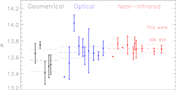
Figure 23. True cluster distance moduli to ω Cen. Black points display distance moduli based on geometrical diagnostics, while blue and red points display distance moduli based either on optical or on NIR distance diagnostics. "S06" and "B16" mark the current overall mean of the distance moduli displayed in Table 7 derived from the theoretical calibration and based on spectroscopic and photometric metallicity distributions, respectively. The horizontal dashed lines display the mean true distance modulus based on the three different approaches. The dotted lines display the dispersions (see Table 8). Note that distances from Cannon (1974) and McNamara (2000) were not used to derive the mean of the optical sample (see text).
Download figure:
Standard image High-resolution imageTable 8. True Distance Moduli to ω Cen: Literature and Current Estimates
| μ | E(B–V) | References | Notesa |
|---|---|---|---|
| mag | mag | ||
| Geometrical (13.56 ± 0.14 mag) | |||
| 13.65 ± 0.12 | ⋯ | Thompson et al. (2001) | (1) |
| 13.75 ± 0.04 | 0.11b | Kaluzny et al. (2002) | (2) |
| 13.41 ± 0.14 | ⋯ | van de Ven et al. (2006) | (3) |
| 13.49 ± 0.14; 13.51 ± 0.12 | 0.131 | Kaluzny et al. (2007) | (4) |
| Optical (13.66 ± 0.07 mag) | |||
| 13.36 ± 0.10 | 0.11 | Cannon (1974) | (5) |
| 13.53 ± 0.20 | 0.11 | Nemec et al. (1994) | (6) |
| 14.02 ± 0.10 | 0.12 | McNamara (2000) | (7) |
| 13.74 ± 0.11 | 0.11b | Caputo et al. (2002) | (8) |
| 13.72 ± 0.11; 13.62 ± 0.11 | 0.11 ± 0.01 | Del Principe et al. (2006) | (9) |
| 13.68 ± 0.27 | 0.12 | Weldrake et al. (2007) | (10) |
| 13.65 ± 0.09 | 0.11 ± 0.02 | Bono et al. (2008) | (11) |
| 13.62 ± 0.05 | 0.16 | McNamara (2011) | (12) |
| 13.71 ± 0.08 ± 0.01 | 0.11 | Braga et al. (2016) | (13) |
| Near-Infrared (13.71 ± 0.05 mag) | |||
| 13.61 | 0.11 | Longmore et al. (1990) | (14) |
| 13.77 ± 0.07 | 0.11 ± 0.01 | Del Principe et al. (2006) | (15) |
| 13.72 | 0.11 ± 0.01 | Sollima et al. (2006b) | (16) |
| 13.75 ± 0.11 | 0.11 ± 0.02 | Bono et al. (2008) | (17) |
| J: 13.65 ± 0.08; H: 13.77 ± 0.08; K: 13.70 ± 0.11 | 0.12 | Bhardwaj et al. (2017) | (18) |
| 13.708 ± 0.035 | 0.12 | Navarrete et al. (2017) | (19) |
| 13.674 ± 0.008 ± 0.038; 13.698 ± 0.004 ± 0.048 | 0.11 | This work | (20) |
Notes.
a(1) Based on the surface brightness method, applied to the detached eclipsing binary V212 to derive the absolute distance to ω Cen (d = 5360 ± 300 pc). (2) Distance based on the surface brightness method, applied to the detached eclipsing binary V212 to derive the absolute distance to ω Cen. (3) Distance based on an axisymmetric dynamical models of the cluster. The models were fitted to the proper motion and radial velocity measurements to provide an estimate of the distance (4.8 ± 0.3 kpc). (4) Distance based on the orbital parameters of the detached eclipsing binary V209. The two distance moduli are for the primary (closest) and for the secondary (farthest) star of the binary system. (5) Distance based on the MV of the Horizontal Branch. (6) Distance based on the B0, −0.3, V0, −0.3 and K0, −0.3 magnitudes of RRLs, where the subscript 0, −0.3 indicates the the reddening-corrected magnitude at . (7) Distance based on the PLV relations of high-amplitude δ Sct stars. (8) Distnce based on the position of the First Overtone Blue Edge of the instability strip in the
  –MV diagram. (9) Distance based on the MV–[Fe/H] relation, calibrated from Bono et al. (2003) and Catelan (2006) for the two values respectively. (10) Distnce based on the MV–[Fe/H] relation, calibrated from Rich et al. (2005). (11) Distance based on the calibration of the TRGB provided by Lee et al. (1993). (12) Distance based on the PLV relations of δ Sct stars. (13) Distance based on semi-empirical and theoretical calibration of the reddening independent PW(V, B–I) relations. (14) Distance based on the K-band PL relation. The relation was calibrated by adopting MK,o,−0.3 = 0.06 and [Fe/H] = −0.24. (15) Distance based on the semi-empirical calibration of the Ks-band PL relation by Bono et al. (2003). (16) Distance based on a new calibration of the Ks-band PL relation. The zero-point was based on the trigonometric parallax of the prototype RR Lyr (Benedict et al. 2011). (17) Distance based on the empirical K-band PL relation provided by Sollima et al. (2008). (18) Distance based on the the J-, H- and K-band PL relations of Type II Cepheids (T2Cs), obtained with a new calibration of the T2Cs in the LMC. (19) Distance based on the J- and K-band PL relations of both RRLs and Type II Cepheids, calibrated with the relations of Alonso-García et al. (2015). (20) Distance based on the J-, H- and Ks-band PLZ relations of RRLs, calibrated with the predicted relations and adopting [Fe/H] from Sollima et al. (2006a) and Braga et al. (2016), respectively.
bThe authors provide (m–M)V and not the true distance modulus μ. Therefore, we adopt E(B–V) = 0.11 and provide μ in column 1.
–MV diagram. (9) Distance based on the MV–[Fe/H] relation, calibrated from Bono et al. (2003) and Catelan (2006) for the two values respectively. (10) Distnce based on the MV–[Fe/H] relation, calibrated from Rich et al. (2005). (11) Distance based on the calibration of the TRGB provided by Lee et al. (1993). (12) Distance based on the PLV relations of δ Sct stars. (13) Distance based on semi-empirical and theoretical calibration of the reddening independent PW(V, B–I) relations. (14) Distance based on the K-band PL relation. The relation was calibrated by adopting MK,o,−0.3 = 0.06 and [Fe/H] = −0.24. (15) Distance based on the semi-empirical calibration of the Ks-band PL relation by Bono et al. (2003). (16) Distance based on a new calibration of the Ks-band PL relation. The zero-point was based on the trigonometric parallax of the prototype RR Lyr (Benedict et al. 2011). (17) Distance based on the empirical K-band PL relation provided by Sollima et al. (2008). (18) Distance based on the the J-, H- and K-band PL relations of Type II Cepheids (T2Cs), obtained with a new calibration of the T2Cs in the LMC. (19) Distance based on the J- and K-band PL relations of both RRLs and Type II Cepheids, calibrated with the relations of Alonso-García et al. (2015). (20) Distance based on the J-, H- and Ks-band PLZ relations of RRLs, calibrated with the predicted relations and adopting [Fe/H] from Sollima et al. (2006a) and Braga et al. (2016), respectively.
bThe authors provide (m–M)V and not the true distance modulus μ. Therefore, we adopt E(B–V) = 0.11 and provide μ in column 1.
Download table as: ASCIITypeset image
The marginal difference between cluster distances based on optical and NIR distance diagnostics might be due to different assumptions concerning cluster reddening and/or zero-point calibrations. Two cluster distances display discrepancies larger than 1σ: one based on an old estimate of the HB luminosity level (μ = 13.36 ± 0.10 mag, Cannon 1974) and another based on the PL relation of δ Sct stars (μ = 14.02 ± 0.10 mag, McNamara 2000). However, this determination is strongly affected by the adopted PL calibration (McNamara 1997). More recent and accurate calibrations (McNamara et al. 2004, 2007) would provide smaller cluster distances.
Finally, it is worth mentioning that remarkable agreement is found with literature estimates based on the TRGB (13.65 ± 0.05 mag, Bono et al. 2008) and on RRLs (13.77 ± 0.07 mag by Del Principe et al. 2006; 13.71 ± 0.08 ± 0.01 mag by Braga et al. 2016; 13.708 ± 0.035 mag by Navarrete et al. 2017).
7. Summary and Final Remarks
In this work we have provided accurate and homogeneous mean optical and NIR magnitudes for a large, unbiased sample of RRLs in ω Cen. The main results obtained from the analysis of the data that we have collected are the following.
Completeness of the RR Lyrae sample. We provide a complete characterization of RRL variables in ω Cen with either unknown or uncertain pulsation mode. See V68, V84, V171, V178, V179, and V182 in the Appendix for more details.
Pulsation period. The time interval covered by our optical and NIR time series data allowed the detection of a period variation for ∼30 RRL variables. The magnitude of these variations typically agrees with specific studies on period change rates (Jurcsik et al. 2001).
Amplitude ratios. The ratios of NIR-over-optical light amplitudes for RRc variables are marginally smaller than for RRab variables. We also found that these ratios are even larger for RRab stars with periods longer than 0.7 days. Interestingly enough, in ω Cen, at periods longer than 0.7 days, there is a paucity of Blazhko RRLs and their amplitude modulation becomes smaller (Braga et al. 2016). It is worth mentioning that the quoted differences are within 1σ.
PLZ relations. The spread in magnitude is consistent with a spread in iron abundance of at least one dex. Moreover, the dispersion is smaller using PLZ relations than when using PL relations. Both are empirical indications that metallicity does affect the zero-point of the PL relation of RRLs.
Distance determinations. We derived the distance modulus to ω Cen from the PLZ(JHKs) relations adopting both an empirical and a theoretical calibration. Moreover, we also adopted two different sets of iron distributions (Sollima et al. 2006a; Braga et al. 2016). True distance moduli based on the theoretical calibration give 13.674 ± 0.008 ± 0.038 mag (spectroscopic iron abundances from Sollima et al. 2006a) and 13.698 ± 0.004 ± 0.048 mag (photometric iron abundances from Braga et al. 2016). These estimates agree quite well (1σ) with recent cluster distance determinations based either on optical or on NIR distance diagnostics. Cluster distances based on geometrical methods, taken at face value, appear systematically smaller than those based on other distance diagnostics.
True cluster distance moduli based on the empirical calibration have errors in the mean that are, on average, a factor of two larger than those based on the theoretical calibration. The current findings support previous results obtained by Neeley et al. (2017) that were based on field and cluster RRLs. There is mounting evidence that the five adopted HST calibrators are affected by systematics at the 5%–10% level.
This is a long-term project aimed at investigating variable stars and stellar populations in ω Cen. We have already performed an optical and an NIR analysis of RRL properties. In a subsequent paper we plan to investigate the metallicity distribution—by providing accurate spectroscopic abundances for a significant fraction of RRLs in ω Cen using high-resolution optical spectra—the reddening distribution, and the distance distribution using both optical and NIR mean magnitudes. These are stepping stones for deriving new NIR (JHKs) light curve templates.
We thank the referee J. Jurcsik for her positive and insightful suggestions that improved the content and the readability of the paper. It is a pleasure to thank J. L. Prieto for his help with time series optical data from ASAS-SN. This publication makes use of data products from the Two Micron All Sky Survey, which is a joint project of the University of Massachusetts and the Infrared Processing and Analysis Center/California Institute of Technology, funded by the National Aeronautics and Space Administration and the National Science Foundation. This publication makes use of data products from the All-Sky Automated Survey for Supernovae that is supported by the Gordon and Betty Moore Foundation through grant GBMF5490 to the Ohio State University and NSF grant AST-1515927. This research has made use of the USNO Image and Catalog Archive operated by the United States Naval Observatory, Flagstaff Station (http://www.nofs.navy.mil/data/fchpix/). This research has made use of NASA's Astrophysics Data System.
Appendix: Notes on Individual RR Lyrae Stars
(V52) This variable shows up, both in CMDs and in PLs in all the literature focused on the RRLs of ω Cen, as an overluminous source. As pointed out by Navarrete et al. (2015) this is due to an unresolved blend with a close companion at 0.5 arcsec, according to HST data (Anderson & van der Marel 2010). We have resolved the blend because, both in the Ks, J–Ks CMD and in the JHKs PLs, it is well within the distribution of the RRLs of ω Cen. This result was achieved by using only LCO15 data, since they were collected with very good seeing (see Table 1).
(V68) Nemec et al. (1994) suggested that this variable is a candidate AC. Recently, Navarrete et al. (2017) claimed that it is not possible to discriminate whether V68 is an RRc or an AC, because it follows both the Ks-band PL relations for RRc and ACs. They adopted the Ks-band PL relation for fundamental (FU) ACs derived by Ripepi et al. (2014) on the basis of ACs in the LMC. However, their relation stops at ∼0.6 days, because FU ACs in the MCs (OGLE, Soszyński et al. 2015) only have periods longer than 0.6 days. Moreover, there is no theoretical evidence (Fiorentino et al. 2006) to support the existence of FU ACs with periods shorter than 0.6 days. Therefore, the PL that should be adopted is that for the FO pulsators (Ripepi et al. 2014). At the period of V68, assuming a distance of μ = 13.69 mag (our paper) and taking account of the reddening, an FO AC should have a Ks-band magnitude ∼12.46 mag. This is ∼0.45 mag brighter than our value for V68 (Ks = 12.942 ± 0.005). This is more than 4σ away from the PL(Ks) relation of FO ACs (σPLK,AC = 0.10 mag, Ripepi et al. 2014). Furthermore, no FU AC is known to be this faint, also in the optical (MV ∼ 0.21 mag). This evidence indicates that V68 is either a background FO AC—but this is in contrast with membership probabilities (100%) derived by van Leeuwen et al. (2000) and Bellini et al. (2009) on the basis of proper motions—or, more probably, that it is a member RRc. If we assume that V68 is an RRc, its period (0.53462524 days) would be among the largest ever found for an RRc in the Halo (GCVs; Samus et al. 2017) and larger than any of the ∼11,000 RRc in the Bulge (OGLE, Soszyński et al. 2014) and of the ∼10,000 in the MCs (OGLE, Soszyński et al. 2016).
(V84) Nemec et al. (1994) suggested that this star is a candidate AC. Recently, Navarrete et al. (2017) claimed, on the basis of the Ks-band PL relations of FU ACs (Ripepi et al. 2014), that it is not possible to discriminate between a foreground RRab and a member AC. For the same reasons already explained in the note of V68, one should use the relation for FO pulsators. If V84 were a cluster member FO AC, its Ks-band magnitude should be ∼12.32 mag. This is ∼0.45 mag brighter than our estimate (12.781 ± 0.009 mag). We rule out the possibility that V84 is a member FO AC. Either it is a background FO AC or it is a foreground RRab. These hypotheses also agree with van Leeuwen et al. (2000), who provides a membership probability of 0% for V84, on the basis of proper motions. Finally, let us mention that we cannot exclude that V84 might be affected by an unresolved blend and new spectroscopic measurements of the radial velocity would be highly desirable to assess the membership of this variable. Interestingly enough, the referee drew our attention to the similarity of the light curve of V84 with the variable V70 in M3 (see Figure 1 in Jurcsik et al. 2015). V70 in M3 is an evolved, overluminous RRc variable with a period of 0.486 days, which is 0.030 days longer than the shortest-period RRab in the cluster.
(V159) The ASAS-SN data are affected by blending, therefore we do not provide an optical mean magnitude, nor an amplitude in Table 3. The comparison with the literature (van Gent 1948,  mag and APh = 0.57 mag, from photographic plates) gives both a brighter mean magnitude (12.395 ± 0.010 mag) and a smaller amplitude AV = 0.072 ± 0.010 mag.
(V171) From ASAS-SN optical data, we have derived the period of this variable (P = 0.52099438 days) for the first time. The period and the sawtooth shape of the light curve tell us that V171 is indeed an RRab star. We have retrieved 2MASS and VHS data and found that V171 obeys the PL relation of the RRLs in ω Cen; we therefore suggest that it is a cluster member.
(V178) The ASAS-SN V-band time series shows no sign of variability. This star should be excluded definitively from the list of candidate RRLs in ω Cen.
(V179) From ASAS-SN optical data, we have derived for the first time the period of this variable (0.50357939 days). However, its light curve is that of an eclipsing binary, with deep minima (∼0.4–0.5 mag) in the V band.
Note that finding charts of V171, V178, and V179 are available (Wilkens 1965). Since their coordinates are more than 50 years old, we have visually inspected the images from the DSS and the finding charts to avoid wrong matches in the modern ASAS-SN, 2MASS, and VHS catalogs.
(V182) This star is marked as an "RR0?" with a period of 0.5454 days and coordinates R.A. = 13:32:13.42 and decl. = −47:06:18.6 in the Clement et al. (2001) catalog. Regrettably, no finding chart is available and the ASAS-SN light curve of the star located at these coordinates shows a constant behavior. However, a star of similar magnitude is located at R.A. = 13:32:18.71 and decl. = −47:06:13.5 (coordinates from the 2MASS Point Source Catalog) and its light curve is sawtooth-shaped with a period of 0.54539506 days. From its period, we conclude that the star that we have found is V182 itself, but its coordinates were wrong. We confirm that V182 is an RRab star, but it is not a cluster member, because its mean J, H and Ks mean magnitudes place it ∼0.4 mag below the PL relation of the RRL stars of ω Cen.
(NV411) This star was missed in our analysis of optical data (Braga et al. 2016) due probably to a mismatch between our point source optical catalog and the catalog of RRLs of ω Cen. The successful match between the catalog of RRLs and our point source NIR catalog allowed us to check again the optical data. Finally, we have retrieved both optical and NIR time series for this star. The UBVRI mean magnitudes and amplitudes of NV411 are listed in Table 3.
Footnotes
- *
This publication makes use of data gathered with the Magellan/Baade Telescope at Las Campanas Observatory, the Blanco Telescope at Cerro Tololo Inter-American Observatory, NTT at La Silla (ESO Program IDs: 64.N-0038(A), 66.D-0557(A), 68.D-0545(A), 073.D-0313(A), ID 073.D-0313(A) and 59.A-9004(D)), VISTA at Paranal (ESO Program ID: 179.A-2010) and VLT at Paranal (ESO Program ID: ID96406).
- 25
This algorithm was implemented in IDL and it is available upon request to the authors.
- 26
This sample includes both RRab and RRc variables. The periods of the latter were fundamentalized, i.e.,
 .
.