


ABSTRACT
We present a consistent optimal estimation retrieval analysis of 10 hot Jupiter exoplanets, each with transmission spectral data spanning the visible to near-infrared wavelength range. Using the NEMESIS radiative transfer and retrieval tool, we calculate a range of possible atmospheric states for WASP-6b, WASP-12b, WASP-17b, WASP-19b, WASP-31b, WASP-39b, HD 189733b, HD 209458b, HAT-P-1b, and HAT-P-12b. We find that the spectra of all 10 planets are consistent with the presence of some atmospheric aerosol; WASP-6b, WASP-12b, WASP-17b, WASP-19b, HD 189733b, and HAT-P-12b are all fit best by Rayleigh scattering aerosols, whereas WASP-31b, WASP-39b and HD 209458b are better represented by a gray cloud model. HAT-P-1b has solutions that fall into both categories. WASP-6b, HAT-P-12b, HD 189733b, and WASP-12b must have aerosol extending to low atmospheric pressures (below 0.1 mbar). In general, planets with equilibrium temperatures between 1300 and 1700 K are best represented by deeper, gray cloud layers, whereas cooler or hotter planets are better fit using high Rayleigh scattering aerosol. We find little evidence for the presence of molecular absorbers other than H2O. Retrieval methods can provide a consistent picture across a range of hot Jupiter atmospheres with existing data, and will be a powerful tool for the interpretation of James Webb Space Telescope observations.
Export citation and abstract BibTeX RIS
1. INTRODUCTION
Retrieval techniques have been used to great effect for several decades to invert visible and infrared spectra of solar system planets and thence infer their atmospheric properties (e.g., Conrath & Gierasch 1986; Fletcher et al. 2009). More recently, these methods have been applied to observations of transiting extrasolar planets (e.g., Lee et al. 2012; Line et al. 2013b; Kreidberg et al. 2014, 2015; Stevenson et al. 2014a; Benneke 2015; Waldmann et al. 2015), although in many cases there has been considerable degeneracy that has prevented the determination of a unique solution (e.g., Barstow et al. 2013b).
Recent observations of transiting hot Jupiters using the Space Telescope Imaging Spectrograph (STIS) and Wide Field Camera 3 (WFC3) on the Hubble Space Telescope (HST) have revealed a variety of atmospheric characteristics. Most notably, the 10 hot Jupiters published in Sing et al. (2016) (for additional details of observations, see Huitson et al. 2013; Line et al. 2013a; Mandell et al. 2013; Pont et al. 2013; Sing et al. 2013, 2015; Wakeford et al. 2013; McCullough et al. 2014; Nikolov et al. 2014, 2015) represent a variety of atmospheres, interpreted as a continuum of clear to cloudy conditions. We demonstrate in this work that STIS and WFC3 spectra together cover a sufficient wavelength range to discriminate between clear atmospheres with sub-solar water abundances, and atmospheres in which the water feature is muted by scattering by clouds.
Sing et al. (2016) find that the relative transit radii in the visible and infrared are good discriminators of atmospheric type. Planets with strong absorption in the visible and weak water vapor abundance features in the near-infrared are likely to be cloudy, whereas those with stronger near-infrared water absorption are likely to have clear atmospheres (Iyer et al. 2016; Sing et al. 2016; Stevenson 2016). However, it is clear that this is a continuum rather than a binary state; so, how do the cloud properties of transiting hot Jupiters vary?
We use an optimal estimation retrieval approach to provide a consistent, data-driven analysis of the 10 hot Jupiter transmission spectra presented by Sing et al. (2016). While optimal estimation does not allow full marginalization over the posterior distribution, it is a fast and efficient method that has proven extremely robust for solar system studies. Indeed, Line et al. (2013c) show that, for spectra that are reasonably well-sampled in wavelength space, the performance of an optimal estimation algorithm is comparable to that of a Differential Evolution Monte Carlo method. We choose simple cloud parameterizations to explore the likely range of cloudy scenarios for each planet. We place constraints on the cloud top pressure, water vapor abundance and cloud optical depth of each planet, with varying degrees of confidence corresponding to the data quality in each case. We compare our findings with those presented by Sing et al. (2016) and discuss our results in the context of cloud formation mechanisms.
2. DATA
All spectral data are taken from Sing et al. (2016) and references therein. For all but 2 of the 10 planets, data from HST/STIS, HST/WFC3 and warm Spitzer/Infrared Array Camera (IRAC) are combined. No WFC3 observations are currently available for WASP-6b or WASP-39b, which means that it is not possible to place such strong constraints on the atmospheres of these two planets. HD 189733b has additional data from HST/Advanced Camera for Surveys (ACS) and HST/Near-Infrared Camera and Multi-Object Spectrometer (NICMOS). The spectral resolution adopted and number of observations vary from planet to planet, with obvious implications for the extent to which each spectrum can be used to constrain atmospheric models.
All spectral data sets presented by Sing et al. (2016) were reduced using consistent systematics models, along with a uniform treatment of limb darkening and system parameters. A common-mode systematics subtraction based on the white light curve for each instrument is used, along with marginalization of the systematics model following Gibson (2014). The authors estimate that this achieves good reliability in the relative transit depths between the instruments to within 1σ, evidenced by the good consistency found between three transits depths measured in the overlapping wavelength regions of the STIS G430L and G750L.
3. MODELING
For this work, we use the NEMESIS radiative transfer and retrieval code, initially developed for solar system planets (Irwin et al. 2008) and subsequently used in several analyses of transiting exoplanet atmospheres (Lee et al. 2012, 2014; Barstow et al. 2013b, 2014). NEMESIS uses an optimal estimation algorithm (Rodgers 2000) to infer the best-fitting atmospheric state vector from an observed spectrum, and incorporates a correlated-k (Lacis & Oinas 1991) radiative transfer model.
We proceed along similar lines to the retrievals of GJ 1214b spectra presented in Barstow et al. (2013b). In transmission geometry, it is reasonable to the first order to neglect multiple scattering, as the majority of photons encountering an aerosol particle are likely to be scattered out of the beam or absorbed, given the very long path length through the atmosphere. Therefore, is it simply the extinction cross-section of any aerosol that matters, and we do not consider any effects of the scattering phase function, which vastly simplifies the parameter space.
Spectral data included in the models are taken from the sources listed in Table 1, and are as used by Barstow et al. (2014). H2–H2 and H2–He collision-induced absorptions are taken from Borysow & Frommhold (1989, 1990), Borysow et al. (1989, 1997), and Borysow (2002).
Table 1. Sources of Gas Absorption Line Data
| Gas | Source |
|---|---|
| H2O | HITEMP2010 (Rothman et al. 2010) |
| CO2 | CDSD-1000 (Tashkun et al. 2003) |
| CO | HITRAN1995 (Rothman et al. 1995) |
| CH4 | STDS (Wenger & Champion 1998) |
| Na | VALD (Heiter et al. 2008) |
| K | VALD (Heiter et al. 2008) |
Download table as: ASCIITypeset image
Optimal estimation, while a fast and efficient method of spectral retrieval, provides only a limited exploration of the posterior due to its dependence on Gaussianity of prior and posterior probability distributions. In order to explore the parameter space as fully as possible, a range of retrievals with different cloud conditions and a priori assumptions are performed for each planet. While this still imposes a restricted parameter space on the problem, we have attempted to make the exploration as unbiased as possible. The values of different model parameters adopted are displayed in Table 2, and the rationale for selecting the parameter space is described further in Section 3.1.
Table 2. Parameter Space for the 3600 Models Used to Fit Each Spectrum
| Albedo | 0 | 0.2 | 0.5 | 0.8 | |||||||||||
|---|---|---|---|---|---|---|---|---|---|---|---|---|---|---|---|
| Gases | H2O | +CO2 | +CO | +CH4 | |||||||||||
| Cloud (top press. in mbar) | Rayleigh | Gray | |||||||||||||
| Extended | C | 103 | 102 | 101 | 100 | 10−1 | 10−2 | U | 103 | 102 | 101 | 100 | 10−1 | 10−2 | U |
| Decade | 102 | 101 | 100 | 10−1 | 10−2 | 102 | 101 | 100 | 10−1 | 10−2 | |||||
| Priors | Cloud | H2O | Na/K | ||||||||||||
| 0.1× | 0.1× | 0.1× | |||||||||||||
| 1× | 1× | 1× | |||||||||||||
| 10× | 10× | 10× | |||||||||||||
Note. Cloud models marked "C" and "U" correspond to clear atmosphere and uniform cloud models, respectively. All cloud models have aerosols distributed with constant specific density in regions of the atmosphere where aerosol is present. The total number of individual retrieval runs, 3600, comes from 25 cloud models, 4 temperature profiles, 4 compositions, and 3 tested a priori values for each of the cloud optical depth, H2O abundance, and Na/K abundance.
Download table as: ASCIITypeset image
3.1. Radiative Transfer
Although the data sets from Sing et al. (2016) have already been analyzed to different degrees, for this work we will make our prior assumptions about each object as unrestrictive as possible. The a priori model atmospheres for each planet are calculated in the same way, using only the information available from knowing the planet's period, mass and radius, and basic properties of the star. The parameter space explored is presented in Table 2.
A key challenge in the interpretation of transmission spectra is the lack of precise information about the temperature structure, and the high degeneracy between temperature and baseline pressure at a reference planetary radius in retrievals (e.g., Barstow et al. 2013a, 2013b). Therefore, we test four temperature profiles for each planet. Each profile corresponds to a different value of the Bond albedo. We calculate each planet's equilibrium temperature using the formula

where T* is the temperature of the stellar photosphere, a is the Bond albedo, R* is the stellar radius, and D is the orbital distance. Approximating the atmosphere as a single slab that radiates equally upward and downward at a temperature Tstrat, the temperature of the slab can be calculated by equating the incoming heat from the star with the outgoing heat from the slab. Assuming an emissivity of unity, this gives the relation

The profile is extended as an adiabat below 0.1 bar, but, in practice, we do not expect this region of the atmosphere to be probed in transmission geometry, so the accessible part of the atmosphere is at a temperature Tstrat.
We also test a variety of simple cloud models. Transmission geometry is especially sensitive to cloud top pressure and particle size. Rather than test a series of different sizes of particles with specific compositions, we test a simple Rayleigh parameterization and a simple gray parameterization. These two extremes correspond to very small, sub-μm sized particles (Rayleigh) and a broad size distribution of large particles (gray). Within each of these categories, we test 12 different vertical distributions of cloud particles: uniformly distributed; cloud top at 1000, 100, 10, 1, 0.1, and 0.01 mbar, with uniform distribution beneath; and cloud top at 100, 10, 1, 0.1, and 0.01 mbar, with the cloud base one decade in pressure below. In each case, where a cloud is present it is distributed with a constant specific density (number of particles per gram of atmosphere) as a function of pressure. We also test a clear atmosphere model with no cloud present.
The effect of each of the cloud models on the spectrum is illustrated in Figure 1. It is clear that higher cloud top altitudes (lower pressures) result in increasingly muted atomic and molecular features in the visible and infrared, and steeper slopes in the visible. For the cases where the cloud only spans a decade in pressure, the lower total optical depth results in a reduced opacity in the red compared with the blue, making the slopes steeper and the gas absorption features clearer. A gray cloud produces much flatter spectra than a Rayleigh scattering cloud, but the effect on the infrared molecular absorption features is similar for both. A Rayleigh cloud has a much stronger effect on the visible spectrum than a gray cloud.

Figure 1. Effect of different cloud properties (extinction as a function of wavelength, cloud top altitude, and cloud extent) on transmission spectra of hot Jupiters produces a varied range of characteristics. The bulk planet properties used are for HD 189733b, and H2O, Na, and K are the only spectrally active gases included.
Download figure:
Standard image High-resolution imageDue to the limited wavelength coverage of the hot Jupiter spectra beyond 2 μm, there is very little information available about the presence of molecular species other than H2O. The two broadband Spitzer/IRAC points provide some indication of the presence or otherwise of absorbers such as CO2, CO, and CH4, but there is insufficient information available in the spectrum to constrain their abundances. To avoid introducing further degeneracy into the problem, we test models with H2O only, then models with H2O plus either CO2, CO, or CH4. Each of these gases alters the relative opacity at the wavelengths probed by Spitzer in slightly different ways (Figure 2).
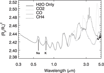
Figure 2. Effects of including CO2, CO, and CH4 on a hot Jupiter transmission spectrum. The H2O-only model (at most wavelengths identical to the H2O+CO model) used is the same as the clear atmosphere model in Figure 1. The addition of extra gases only has measurable effects at the wavelengths probed by Spitzer (and HST/NICMOS for HD 189733b). The locations of the Na and K features at optical wavelengths are indicated.
Download figure:
Standard image High-resolution image4. RESULTS
We present the results of 3600 retrievals for each of the 10 hot Jupiters in the Sing et al. (2016) survey. The full results for each planet are provided as supplementary material; here, we focus only on the 2% of tested models that provide the best fits to the observed spectra.
We use the reduced χ2 statistic ( ) to evaluate the goodness of fit in each case. This is defined as the χ2 divided by the number of degrees of freedom—in this case, the number of spectral points minus the number of retrieved parameters in each model run. Models containing an additional molecular absorber to H2O have one less degree of freedom, so they are penalized for additional complexity. We then rank each model run according to
  , with lower
  values providing the best fits to the measured spectrum. The ranking is performed by calculating ln(
 ) and then normalizing, such that the range for each planet is between 0 and 1. Full retrieved results against normalized ln(
 ) are provided as supplementary material (Section
The best model fits to the spectra (normalized ln( ) < 0.05) are presented in Figure 3. The models are shaded from dark (best) to light (poorest) fitting based on the reduced χ2. Spectra with larger error bars can clearly be fit by a broader range of model properties, with a lack of HST/WFC3 data clearly removing constraint on the shape of the 1.4 μm water band for WASP-6b and WASP-39b. For some planets, fitted spectra clearly fall into two distinct categories (e.g., HAT-P-12b, which has one class of solutions with a more opaque cloud and a second with lower opacity in the red), showing that the model parameter space is bimodal.
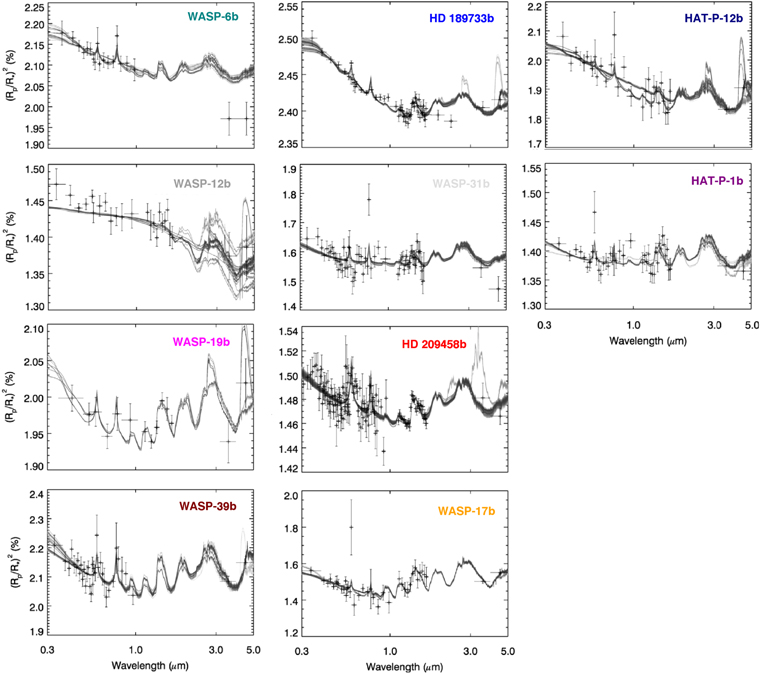
Figure 3. Model fits for the best-fitting models in each case to the observed spectra for each planet. We include only models with a normalized ln( ) < 0.05. The best-fit models are shaded almost black, with the models that fit less well presented in lighter shades of gray. The width of each spectral channel is indicated by a horizontal bar.
Download figure:
Standard image High-resolution imageFor the most part, spectra are well represented by at least some models within the family tested. There are, however, exceptions for specific parts of some data sets. The Spitzer points for WASP-6b have extremely low transit depths compared with the STIS measurement; the lack of WFC3 data for this planet makes it difficult to determine whether this offset is real, or if it is due to an uncorrected systematic effect. The spectral fits shown here do not provide a good match to these data points, but the IRAC points for WASP-6b are derived from incomplete transits (Nikolov et al. 2014), so they may be considered less reliable than the STIS data. A better match would be possible for a model with an extremely opaque, high cloud, but these models do not show any Na or K absorption features as, to fit the Spitzer points, the cloud needs to be so opaque and high up that these are obscured completely. An example of this kind of model can be seen in Figure 1 of Sing et al. (2016). We chose the set of solutions presented here on the assumption that the detection of Na and K is more robust than the IRAC data points.
Another clear discrepancy can be seen in the WASP-31b spectrum, where the 4.5 μm IRAC data point cannot be fit by any models in the family. It is difficult to find a scenario in which the 4.5 μm IRAC point has a transit depth so much smaller than both the 3.6 μm point and the WFC3 data, and the same issue can be seen in Figure 1 of Sing et al. (2016). In general, the error bars on the IRAC points are larger than those on the STIS points, but the individual points carry increased weight as they provide the only information available at wavelengths longer than 2 μm. We expect statistical fluctuations of up to 2σ in 5% of these points. However, given their significance, such random fluctuations can have a large effect on the retrieval and interpretation, and this should be kept in mind.
Finally, the NICMOS points for HD 189733b are not well reproduced by any model within our suite. The opacity in this spectral region is largely provided by collision-induced absorption of H2 and He, so it is difficult to think of a scenario in which this opacity could be removed. The HD 189733b models already have significant cloud opacity with a high top pressure, so a scenario in which the opacity at shorter wavelengths could be increased sufficiently to allow a fit to all of the STIS, ACS, WFC3, and NICMOS points seems unlikely. The discrepancy between the models we show here and those presented by Sing et al. (2016) has been traced to a lack of sufficient collision-induced absorption in the models shown by Sing et al. (2016; J. Fortney 2015, private communication). The shortest wavelength STIS points are also not well represented in some cases, with the models appearing to lack sufficient absorption at these wavelengths. We note that while we have assumed a uniform temperature for the retrieval, detailed analysis of the sodium line has revealed a hot thermosphere at the upper atmospheric layers for this planet (Huitson et al. 2012; Wyttenbach et al. 2015).
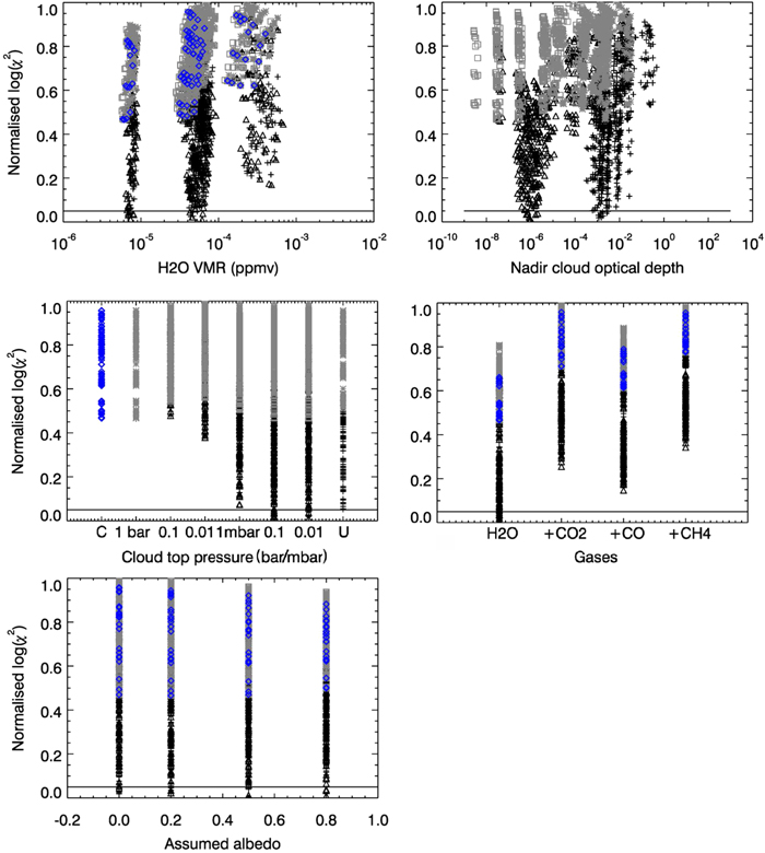
The properties of the best-fitting models are shown in Figures 4 and 5. Each panel in Figure 4 explores the parameter space between two model variables to highlight any correlation between properties. Variables with a lot of scatter are indications that there is limited constraint from the spectrum. Figure 5 shows best-fitting model properties by planet.
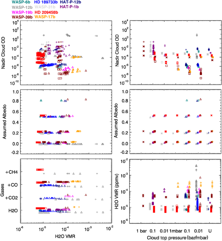
Figure 4. Model parameters where normalized ln( ) < 0.05. Colors correspond to the labels for each planet in Figure 3. Symbols correspond to the different flavors of cloud model, crosses are extended Rayleigh scattering models, asterisks are extended gray models, diamonds are clear atmosphere models, open triangles are decade-confined Rayleigh models, and open squares are decade-confined gray models. The different plots highlight correlations between different model properties. Points are shifted slightly for each planet for quantities with discrete values, such as cloud top pressure.
Download figure:
Standard image High-resolution image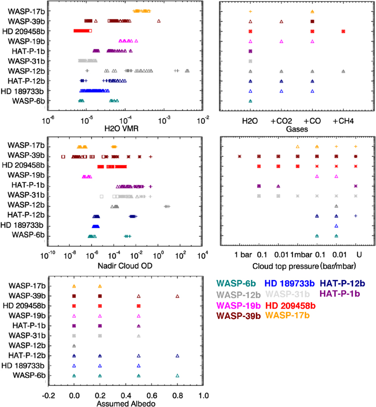
Figure 5. Model parameters where normalized ln( ) < 0.05, by planet. Symbols correspond to the different flavors of cloud model, crosses are extended Rayleigh scattering models, asterisks are extended gray models, diamonds are clear atmosphere models, open triangles are decade-confined Rayleigh models, and open squares are decade-confined gray models. The different plots highlight correlations between different model properties. Points are shifted slightly for each planet for quantities with discrete values, such as cloud top pressure.
Download figure:
Standard image High-resolution image4.1. H2O and Other Molecular Absorbers
H2O abundances cluster between 0.01 × solar values and solar values. HD 209458b has the lowest abundance, between 5 and 10 ppmv. WASP-17b has the highest constrained abundance, between 100 and 600 ppmv. The solar value is approximately 500 ppmv. No constraint on H2O abundance is obtained for WASP-12b, as no water feature is clearly visible in the spectrum, and, for some models, the cloud optical depth is so high that none would be visible. For WASP-6b and WASP-39b, for which there are no WFC3 measurements, only a rough upper limit on H2O abundance is obtained, with this limit emerging from the facts that no H2O absorption features are observed in the long wavelength part of the STIS spectrum, and the Spitzer levels imply molecular absorption.
The presence or absence of other molecular species can be constrained to some extent by the relative transit depths at the wavelengths probed by Spitzer/IRAC at 3.6 and 4.5 μm. However, due to the degeneracy inherent in using two data points to provide information about three gases, it is impossible to place any limits on the abundances of these gases. Figure 2 demonstrates that CO2 would have low absorption at 3.6 μm, but strong absorption at 4.5 μm, whereas the opposite would be true for CH4. For H2O, only the 4.5 μm absorption is slightly stronger than 3.6 μm, with this effect slightly further pronounced for CO. Because the effect of CO is small, its presence is hard to rule out, but CO2 and CH4 are more straightforward.
WASP-31b, WASP-6b, and HAT-P-1b are fit best by models with H2O only. WASP-12b does not have strong constraints on the presence of other gases. WASP-17b is best matched by models with either H2O only or H2O plus CO. HD 209458b can be fit by any models except those containing CO2. HD 189733b, WASP-19b, WASP-39b, and HAT-P-12b can be fit well with any model except those containing CH4. In aggregate, these findings are compatible with the likelihood of hot planetary atmospheres having CO-dominated carbon chemistry over CH4, as the majority of constraints are in favor of either the presence of CO, a lack of any gas except H2O (which, given the small effect of CO, does not provide strong evidence to rule it out), or a lack of CH4.
4.2. Clouds
The clearest division between groups of planets lies in the Rayleigh cloud and gray cloud planets. HD 209458b, WASP-31b, and WASP-39b are all fit best by gray models (asterisks or squares in Figure 4), whereas the other planets are better represented by a Rayleigh scattering cloud (crosses or triangles). HAT-P-1b is the only planet with roughly equal sets of solutions for both gray and Rayleigh cases, although WASP-31b and WASP-39b both have a handful of Rayleigh solutions, as well as gray solutions. No planet is fit well with a completely clear atmosphere model, except for a small minority of models for WASP-39b (diamonds).
Cloud top pressures are tightly constrained for some planets, but not for all. HD 189733b, HAT-P-12b, WASP-6b, and WASP-12b have clouds with a top pressure of 0.1 mbar or below, indicating that there is strong evidence for a cloud high in the atmosphere. Unsurprisingly, these planets all also have results strongly in favor of Rayleigh scattering clouds, which makes intuitive sense, as it is easier to loft small particles to high altitudes within an atmosphere. WASP-17b and WASP-19b, the other two planets with solutions favoring a Rayleigh cloud, have cloud top pressures of 1 mbar or lower. HAT-P-1b has the deepest cloud, with top pressures between 0.1 and 0.01 bar, consistent with either a gray or Rayleigh cloud.
Planets that have mostly gray cloud solutions have much broader ranges of acceptable cloud top pressures. HD 209458b has a cloud top range between 0.01 bar and below 0.01 mbar. The lower cloud top pressures make less intuitive sense in this case, as a gray cloud must contain some large particles and these would be unlikely to be lofted very high, especially as the optical depth for HD 209458b is in the middle of the range spanned by all planets. WASP-31b has a similar range and optical depth. WASP-39b has a slightly more logical correlation between cloud top pressure and optical depth, with a low optical depth family of solutions for 0.1 and 0.01 mbar cloud top pressures and a higher optical depth set of solutions for 1 and 0.1 bar cloud tops.
HD 189733b has strong evidence in favor of a decade-confined Rayleigh scattering cloud. If this is a vertically confined aerosol layer high in the atmosphere, it would suggest either a species that condenses at cool temperatures only found high up, or a photochemically produced haze that is short lived deeper in the atmosphere. It is not known what kinds of photochemical products could form and be stable at HD 189733b temperatures.
One trend that we uncover is that the coolest (WASP-6b, HAT-P-12b, HD 189733b, Teq < 1300 K) and hottest (WASP-12b, WASP-17b, WASP-19b, Teq > 1700 K) planets are the ones that have good evidence for relatively high Rayleigh scattering aerosols (Table 3). WASP-39b is also relatively cool, but gray cloud models are favored. The intermediate temperature planets (HD 209458b and WASP-31b, with 1300 K < Teq < 1700 K) are all also best fit by gray cloud models. HAT-P-1b is fit best by Rayleigh scattering models, but only deep clouds are favored, so there is little sensitivity to the scattering properties of the cloud. This suggests that a clearing of clouds may occur at this temperature. Taking the cloud top pressures that occur most frequently within the best-fitting models, the planets with gray cloud solutions (except WASP-39b) are more likely to have deeper clouds, which makes intuitive sense, as larger particles are less likely to be supported higher up in the atmosphere.
Table 3. Evidence of a Possible Relationship between Equilibrium Temperature and Cloud Properties for this Family of Hot Jupiters
| Planet | Teq (K) | Rayleigh/Gray | Ptop (mbar) |
|---|---|---|---|
| HAT-P-12b | 963 | R | 0.01 |
| WASP-39b | 1117 | R/G | 0.01 |
| WASP-6b | 1145 | R | 0.01 |
| HD 189733b | 1201 | R | 0.01 |
| HAT-P-1b | 1322 | R | 100 |
| HD 209458b | 1448 | G | 10 |
| WASP-31b | 1575 | G | 100 |
| WASP-17b | 1738 | R | Top |
| WASP-19b | 2050 | R | 0.01 |
| WASP-12b | 2530 | R | 0.01 |
Note. Equilibrium temperatures are taken from Kataria et al. (2016), except for that of WASP-12b, which is calculated for this work using system values provided by Sing et al. (2016). The best-fit Ptop quoted is the most commonly occurring value within the models where normalized ln(χ2 < 0.05).
Download table as: ASCIITypeset image
This may possibly indicate a continuum of cloud formation through different mechanisms, or from different substances. We show a schematic outlining these trends in Figure 6. As atmospheres cool, a cloud formed from the same condensate will gradually fall deeper in the atmosphere, and eventually new species will condense out forming new clouds in the upper regions of the atmosphere. A similar sequence has been postulated for brown dwarfs (Lodders & Fegley 2006, pp. 1–28). This sequence can explain both the trends in scattering properties and the trends in cloud structure that we see as a function of temperature. In particular, note that of the hot and cold groups of planets with a Rayleigh scattering cloud high in the atmosphere, WASP-6b and HD 189733b, and WASP-19b and WASP-12b, all favor models where the cloud is confined to a limited pressure range in the atmosphere, whereas WASP-17b and HAT-P-12b both favor extended cloud models.
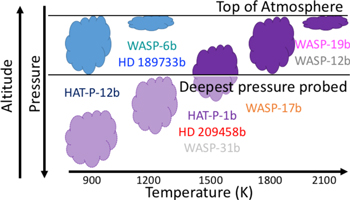
Figure 6. Schematic illustrating how cloud structure for these hot Jupiters may vary with temperature, inferred from our retrieval results. For the hottest planets in the sample, WASP-19b and WASP-12b, the condensate we see can only exist relatively high in the atmosphere. For slightly cooler planets, such as WASP-17b, the cloud that originally forms high up in the atmosphere can extend downwards. Eventually, the cloud particles become large enough to sediment out and the cloud is only seen deep in the atmosphere (WASP-33b, HD 209458b, HAT-P-1b). For even cooler atmospheres, new species start to condense out and the sequence is repeated (WASP-6b, HD 189733b, HAT-P-12b).
Download figure:
Standard image High-resolution imageAt cooler temperatures near ∼1000 K, the expected condensible species of MnS, Na2S, and KCl are all highly scattering, while at temperatures near 1500 K iron clouds could form, which may be more gray (Wakeford & Sing 2015). Further observation will be necessary to test the effect of stellar proximity, and therefore temperature, on hot Jupiter cloud formation. An important question is whether other hot Jupiters also follow this trend, which will be the subject of future work.
Stevenson (2016) found correlation between muted water vapor features in WFC3 spectra and the planet's location in temperature–log(g) space. Planets with higher equilibrium temperature or log(g) are found to have stronger water vapor features than those with low temperature and log(g), which is interpreted as a greater likelihood of obscuring cloud in cooler/puffier planets. This makes intuitive sense, as clouds are more likely to condense in cooler atmospheres and less likely to sediment out in lower gravity atmospheres.
We reproduce Figure 2 from Stevenson (2016) with data for the 10 planets in this study (Figure 7). The dashed line indicates the demarcation between weak/strong H2O features as found by Stevenson (2016). However, we do not find any correlation between position in this parameter space and the presence or absence of clouds high in the atmosphere. This may be a result of the small sample sizes used in each case, and also the fact that Stevenson (2016) include small planets in the sample whereas we only study hot Jupiters.

Figure 7. Ten planets in this study shown in effective temperature–log(g) parameter space. The dashed line indicates the demarcation between weak and strong H2O features, which is suggested as a possible proxy for cloudiness by Stevenson (2016). The squares with crosses marked are those from our sample for which clear/deep cloud models provide the best fit. Uncrossed squares are planets for which a high cloud is favored, although for WASP-17b and WASP-19b, this cloud is likely to be optically thin.
Download figure:
Standard image High-resolution imageThe lack of agreement in our results may in part be due to differences in the reduction of data, which is particularly notable for HD 189733b. This difference is discussed in more detail in Section 5.2. However, this also suggests that data in the STIS wavelength range are important for discriminating between clear and cloudy atmospheres, as well as the WFC3 region.
4.3. Temperature
The assumed albedo, a proxy for temperature (zero corresponds to zero dayside albedo, and the same temperature at the terminator as on the dayside) is poorly constrained for most planets, as the temperature has a relatively small effect on the shape of the spectrum, which is degenerate with the radius at the 10-bar pressure level. However, for all planets except HAT-P-12b, WASP-39b and WASP-6b, an albedo proxy of 0.8 or higher is ruled out. For WASP- and WASP-17b proxies of 0.5 or higher are ruled out. This generally favors low albedo and efficient recirculation.
4.4. Comparison With Sing et al.
Sing et al. (2016) use empirical spectral indices, including the size of the H2O feature and the near-IR to mid-IR slope, to form an initial categorization of the 10 planets. In general, the trends uncovered are borne out by this retrieval analysis. However, whereas Sing et al. (2016) did not find evidence for any trend with temperature, our more detailed analysis is able to show that the structure, and probably the composition, of the cloud on these planets changes with increasing temperature.
WASP-19b and WASP-17b are labeled as the clearest atmosphere planets by Sing et al. (2016). In our analysis, both planets have Rayleigh scattering aerosol that can exist to quite low pressures, but higher H2O abundances than the majority of planets. These planets do not have completely clear atmospheres, but the aerosol that is present does not impact our ability to identify infrared molecular absorption. There is an important distinction to be drawn between hazy planets like this, and those with more opaque clouds, such as HD 189733b.
There is some correlation between the type of cloud that provides the best fit and the cloud coverage ordering presented by Sing et al. (2016). The planets Sing et al. (2016) determined to be the cloudiest—WASP-6b, HD 189733b, HAT-P-12b, and WASP-12b—are all best represented in our analysis by Rayleigh scattering clouds with relatively low top pressures. In general, and excepting WASP-19b and WASP-17b, the planets categorized as less cloudy by Sing et al. (2016) are more likely to be represented by gray cloud models with flatter spectra. This makes sense, as one of the key spectral indices in determining cloudiness is the overall slope from the optical to the mid-infrared, which is stronger for Rayleigh scattering clouds than for gray. Sing et al. (2016) also found that HD 209458b, and to some extent WASP-31b, lie closer to their "cloudy" models (gray cloud parameterization) instead of the "hazy" models (Rayleigh scattering cloud parameterization). WASP-39b, another gray cloud planet in our analysis, also has a very shallow downward or possibly even upward slope from the optical to the mid-infrared. These indices appear to be fairly robust discriminators of gray versus Rayleigh scattering aerosols and can determine which planets will have large IR molecular features in their transmission spectra, but degeneracies make it difficult to use similar techniques to rule out the presence of aerosol altogether.
We do not show results for Na and K abundances, as although these were retrieved, results were generally inconclusive. We also found some difficulty in fitting the precise shapes of these bands, as the centers of the features are very narrow and the absorption tables used have a limiting resolving power of 100 at 500 nm. Retrieved abundances of CO2, CO, and CH4 are also not presented, as precise constraints were not obtained.
5. DISCUSSION
Our ability to fit the spectra of 10 very different hot Jupiters using the same basic model demonstrates the power of spectral retrievals to explore the atmospheres of transiting exoplanets. However, it is clear that there is still significant degeneracy within the data set, and a good fit is harder to achieve for some planets than others. Here, we briefly discuss the cases for which a more planet-specific approach might be supposed to yield a better fit quality.
5.1. WASP-31b
WASP-31b is the only candidate planet in the sample that is fit best by Sing et al. (2016) with a multi-modal cloud model. A two-component cloud provides a Rayleigh scattering slope at short wavelengths and a flat spectrum at longer wavelengths. The model set used in our investigation did not include multi-modal clouds, although the presence of such a cloud is plausible—Venus provides the best solar system example (e.g., Knollenberg 1982).
We test the effect of introducing a multi-modal clouds for retrievals of WASP-31b. We include both a gray "cloud" and a Rayleigh scattering "haze." Haze top pressures of 0.01 mbar, 0.001 mbar, and a uniform haze were tested, and for each of these, cloud top pressures up to 0.01 mbar were tested (except for the 0.01 mbar haze top case, for which the cloud only extends up to 0.1 mbar).
Although the apparent shape of the spectrum seems to favor this kind of two-component model, the reduced χ2 values do not provide any strong evidence for this over a simpler model. Two-component cloud model plots are shown in Figure 8, with the lowest reduced-χ2 values actually slightly higher than those of the best-fitting single-cloud models.
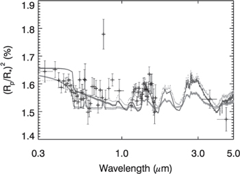
Figure 8. WASP-31b spectrum with two-component cloud models. Solid lines show haze with a top pressure of 0.01 mbar, dotted lines show has with a top pressure of 0.001 mbar. Darker shades correspond to lower cloud top pressures. None of these models produce a substantially better fit to the spectrum.
Download figure:
Standard image High-resolution image5.2. HD 189733b
The data for HD 189733b are probably the most constraining of the 10 planets. However, there are some clear discrepancies between the models and the observed spectrum. The most obvious is the very low transit depth for the two NICMOS points in the 2 μm region.
The binned NICMOS points used in this paper are as presented by Pont et al. (2013), but they were binned up from a spectrum that was originally reduced by Gibson et al. (2012). This original spectrum has large error bars and also a large amount of scatter. If the original spectrum from Gibson et al. (2012) is overplotted (Figure 9), it can be seen that the majority of points longwards of 1.6 μm match the models quite well. The averaged points have their transit depths brought down by three low values at the shortest wavelength end, and two outlying low points at longer wavelengths. The transit depths were fractionally reduced by the star-spot correction applied by Pont et al. (2013), and subsequently the models do not provide quite such a good match to the data.
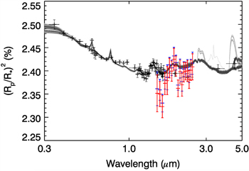
Figure 9. HD 189733b model spectra, plus data including the full NICMOS spectrum from Gibson et al. (2012; blue) and as modified by Pont et al. (2013; red). There is an obvious mismatch with the WFC3 spectrum and models at the bluer end of the NICMOS range, but moderate agreement with models elsewhere due to the large error bars on the spectrum. The broad spectral shape is consistent with absorption by H2O + H2–H2 collision-induced absorption, as shown in the models.
Download figure:
Standard image High-resolution imageIt is impossible to fit the binned points with any plausible model spectrum. In order to simultaneously fit the Rayleigh-dominated slope in the STIS and ACS data and the small water feature, a fairly low H2O abundance is required. This means that H2–H2 collision-induced absorption features become visible between the water bands, providing a hard opacity floor. Even if the spectrum could be fit with a combination of Rayleigh cloud and gray cloud, as suggested for WASP-31b, which would potentially allow H2O abundances closer to the solar value, the opacity floor would still fall above the NICMOS points as the longer wavelength H2O features would then be stronger.
Given the complicated systematics of the NICMOS instrument, discussed at length by Gibson et al. (2012), and especially in the light of the obvious discrepancy with WFC3 results at the shorter wavelength end, we conclude that the lack of a good match to these points does not provide strong evidence of inaccuracies in our best-fit model.
5.2.1. Star Spots and Spectral Stitching
Each of the spectra in this survey were compiled from segments of spectrum obtained by different instruments at different times. As discussed by Pont et al. (2013) in the context of HD 189733b, and Barstow et al. (2015) with a view toward JWST, changing star-spot coverage between the times when different data sets were obtained can affect the accuracy of spectral stitching. Pont et al. (2013) describe star-spot corrections for stitching of HD 189733b, based on ground-based monitoring of the stellar flux over several years. Individual spectral points are shifted up or down depending on the relative numbers of occulted and unocculted spots estimated to be present at the time of observation, as, especially in the visible, the effect of star spots increases toward shorter wavelengths. A strong downward slope from visible wavelengths through to the infrared remains even after correction for star spots.
McCullough et al. (2014) postulate that it is possible to explain the broad spectral shape of the HD 189733b observations with star spots alone, without invoking the presence of clouds, and, under this assumption, they were able to fit the spectrum with a clear solar composition atmosphere model. Their hypothesis assumes a more significant effect from unocculted star spots (spots outside the transit chord) compared with occulted spots, and also a more substantial effect than that estimated by Pont et al. (2013), which was arrived at by monitoring the star and analyzing occulted star spots in transit light curves. This is a difficult question to resolve, since the spot coverage when HD 189733 is at its brightest is an unknown quantity.
However, HD 189733b is the most active star in the data set considered here. A common proxy for stellar activity is the log[CaHK] value, which is a measure of the emission in the H and K Fraunhofer lines from singly ionized calcium. HD 189733b has a log[CaHK] value of −4.501, higher than the values for the other stars in this study; despite this, other transmission spectra display slopes of similar magnitude in the visible, including those of planets such WASP-12b and HAT-P-12b, which have log[CaHK] values of less than −5. This, combined with the fact that very substantial spot coverage needs to be invoked to explain the slope for HD 189733b, would indicate that the presence of aerosol is a more likely explanation for these slopes. We believe that the evidence from HD 189733b indicates that spots could probably not reproduce this same effect across planets orbiting less active (and by extension less spotty) stars.
5.3. WASP-12b
As discussed by Sing et al. (2013), the WASP-12b transmission spectrum is extremely challenging to fit with Rayleigh scattering cloud models. The best fit obtained by Sing et al. (2013) over a range of atmospheric temperatures is for Mie scattering Al2O3. Fits using Rayleigh scattering particles are hampered by the requirement for low atmospheric temperatures of around 800 K, which seems to be incompatible with WASP-12b's expected high equilibrium temperature.
We find that the best fits from our limited model set are provided by an optically thick Rayleigh scattering aerosol with a 0.01 mbar top pressure, but the quality of fit decreases toward shorter wavelengths, with more opacity required than is provided by any of the models. Rather than finding a trend toward cooler atmospheric temperatures, we actually find a fit consistent with a zero dayside albedo and strong recirculation—hot atmospheres are strongly favored for this planet. It is likely that more complex Mie scattering clouds may provide a better fit to the observed spectrum, but there would be significant degeneracy between various cloud parameters, so a detailed exploration will most likely be deferred until after observation with JWST.
Kreidberg et al. (2015) recently published a new WFC3 transmission spectrum for WASP-12b, with increased precision. These results show a clear H2O detection. Analysis in the paper, including with the NEMESIS code, found H2O volume mixing ratios between 10 and 10,000 ppmv, and analysis with the CHIMERA code (Line et al. 2013b) ruled out an atmosphere with C:O >1 at 3σ confidence.
We do not attempt to perform a retrieval with these data due to the difficulty of combining different analyses using different limb darkening and system parameters. Figure 10 shows that there is a clear offset between the new WFC3 data and the previously obtained spectrum. In addition, all data we consider from Sing et al. (2016) have been reduced using the same light-curve analysis pipeline, and this would be required for a rigorous analysis of the new WFC3 data in the context of STIS and Spitzer measurements. However, it is clear from Figure 10 that the observed water vapor feature from Kreidberg et al. is larger than the feature predicted by any of our best-fit models. To fit this feature, models would need one or more of the following modifications: a substantially increased H2O abundance, a reduced cloud optical depth, or a hotter upper atmosphere resulting in an increased scale height. As stated above, an optically thick cloud appears to be required by the steep slope in the STIS measurement, and it would not be expected for such a hot planet to have a substantially super-solar H2O abundance. The temperature of the upper atmosphere, to which thermal emission measurements are relatively insensitive (Stevenson et al. 2014b), is the least well-constrained property here. Future analyses with consistently reduced data and a greater range of temperature profiles may shed further light on this planet.

Figure 10. WASP-12b spectra including the newer WFC3 spectrum from Kreidberg et al. (2015). There is an obvious offset between this spectrum and the existing data, resulting from differences in the system parameters and limb darkening used in the analysis. This is a common issue in transit spectroscopy and was discussed by Kreidberg et al. (2015).
Download figure:
Standard image High-resolution image5.4. Influence of Spitzer Data
The Spitzer data provide the only information at wavelengths >2 μm in these retrievals, and, as such, they provide a critical role in our conclusions about the presence of molecular species other than H2O. However, there has been considerable debate about the reliability of Spitzer photometry in the past, with reanalyses producing substantial shifts in transit depths (e.g., Diamond-Lowe et al. 2014; Evans et al. 2015) and conclusions drawn from only two points are obviously highly degenerate.
We test the influence the Spitzer data on our results by running the retrievals again without the Spitzer points. The results are presented in Figure 11. There are few substantial differences between these results and the originals (Figure 5), including the Spitzer data. The key differences are (1) removing the Spitzer data for HAT-P-1b means that this planet is better fit by gray cloud models than Rayleigh scattering models; and (2) a reduction in our ability to draw conclusions about the presence of molecular species other than H2O. The second of these consequences is entirely to be expected, since the only information we have about these other gases comes from the Spitzer points.

Figure 11. Model parameters where normalized ln( ) < 0.05, by planet, for retrievals without the Spitzer data. Symbols correspond to the different flavors of cloud model; crosses are extended Rayleigh scattering models, asterisks are extended gray models, diamonds are clear atmosphere models, open triangles are decade-confined Rayleigh models, and open squares are decade-confined gray models. The different plots highlight correlations between different model properties. Points are shifted slightly for each planet for quantities with discrete values, such as cloud top pressure.
Download figure:
Standard image High-resolution imageWASP-39b and WASP-6b favor H2O-only models when the Spitzer points are removed; however, these two planets now only have STIS data, meaning that no molecular species are detected at all. This is, therefore, simply a consequence of a penalty on the reduced-χ2 when an extra model parameter is included. In conclusion, the Spitzer points do provide some constraint for some planets on the presence of molecular species other than H2O, but have relatively little influence on any other retrieved parameters, and therefore have little bearing on our conclusions about the cloud properties of these worlds, with the exception of gray versus Rayleigh scattering on HAT-P-1b.
5.5. Comparison with Climate Models
Kataria et al. (2016) present a General Circulation Model (GCM) survey of 9 of the 10 hot Jupiters discussed here. WASP-12b is deferred to a later study due to its high equilibrium temperature. This study is based on the Substellar and Planetary Radiation and Circulation model (Showman et al. 2009). The model is cloud-free and calculates temperature structure, wind fields, and gas mixing ratios across the planet. Here, we compare the model predictions from Kataria et al. (2016) with the retrieval results in this work.
5.5.1. Gas Abundances
The gas abundances in the GCMs are derived from solar composition (after Lodders 2003) thermochemical equilibrium models. As all planets are hot, CO chemistry is expected to generally dominate over CH4 chemistry, so the two most abudant molecular species after H2 are H2O and CO. CO2 has very low abundances for all planets and the CH4 abundance decreases from potentially observable levels at the terminators for the coolest planets (HAT-P-12b, WASP-39b, WASP-6b, and HD 189733b, with equilibrium temperatures below 1300 K) to levels several orders of magnitude below CO for the others.
The spectral data available provide limited constraint on the presence of gases, except H2O. However, the H2O abundances from the retrievals are sub-solar (by between 1 and 2 orders of magnitude) for the majority of the 10 planets in our retrievals. WASP-17b is the exception, with an approximately solar H2O (a volume mixing ratio of ∼5 × 10⁻⁴).
Despite a generally lower H2O volume mixing ratio than a solar composition atmosphere, as mentioned above, our results are consistent with CO-dominated carbon chemistry. We see no evidence for CH4 absorption for any planet, and the only planets for which any solutions including CH4 are possible are WASP-12b (which, although not dealt with in the GCM study, is almost certainly too hot to have substantial CH4) and HD 209458b. With the caveat that constraints on the presence of CO2, CO, and CH4 are not strong, and depend heavily on the Spitzer points, this would suggest that CO chemistry dominates on all planets in the sample, including the cooler ones, and therefore disequilibrium effects may be important.
5.5.2. Condensate Formation
Kataria et al. (2016) also included estimates of which condensates are likely to form at different pressure levels on each planet. This is of particular interest for HD 189733b, which has strong evidence for a vertically confined cloud. Based on these models, condensates that would only form at low pressures could be KCl or ZnS (western terminator profile) or Na2S (eastern terminator profile). These particles have somewhat different properties to MgSiO3 (enstatite), which has previously been considered as a possible condensate on HD 189733b. Lee et al. (2014) found that Na2S is consistent with the terminator spectrum of HD 189733b.
Condensate cloud formation is very heavily dependent on the spatially varying temperature profile and also on circulation, for which we currently have very little constraint. In addition, the majority of models simply consider the condensation curve at equilibrium when calculating the height of cloud condensation. Constraints on cloud structure, such as those obtained for HD 189733b, can start to inform directions of research for exoplanet cloud models, but the higher spectral quality of JWST will most likely be required for significant advances. Wakeford & Sing (2015) demonstrate how the increased spectral resolution and coverage of JWST spectra can further constrain cloud properties.
Wakeford et al. (2016) summarize the condensation temperatures of a variety of possible hot Jupiter cloud constituents, along with the available masses of each condensate. For temperatures greater than 1700 K, the majority of possible condensates are Ti and Al compounds, with Ti and Al being the limiting species for these cloud constituents. Below this temperature, the condensates with the highest available masses are Fe and and magnesium silicate minerals; these available masses outnumber those for Al-based compounds by an order of magnitude and Ti based compounds by a factor ∼100. The theoretical condensation temperatures do not correspond exactly to the temperatures where we observe transitions between the cloud types. However, it is conceivable that the reason the hotter planets with extended clouds (WASP-17b, WASP-19b, and WASP-12b) tend to have lower cloud optical depths and more visible molecular features than the colder planets is simply that the available mass for the hotter condensate is lower than that for the colder condensate.
5.5.3. Hemispheric Asymmetry
Kataria et al. (2016) predicted substantial hemispheric asymmetry in temperature and chemistry for many of the planets in the sample. This is a consequence of the strong eastward jets that are thought to occur on tidally locked hot Jupiters. Evidence for these jets is found in the offset of thermal phase curve hot spots (e.g., Knutson et al. 2012; Stevenson et al. 2014b) and is predicted by GCMs.
Kataria et al. (2016) found that, in general, the eastern terminator region is relatively warm, but for all but the most highly irradiated planets, the western terminator is actually the coldest region on the planet. Our retrieval models are one-dimensional, so we are effectively representing an average of two potentially very different limbs. These large temperature differences between the limbs raise the possibility of cloud material condensing out at different pressure levels on different limbs. An extreme case would be one cloud-free limb and one cloudy limb.
Line & Parmentier (2016) explore the impact of this extreme scenario, and found that partially cloudy models can produce very similar WFC3 spectra to cloud-free models with a high mean molecular weight atmosphere. Given the size and temperature of the objects we consider in this study, it is most likely that they are all H2–He-dominated; however, it is possible that their east and west limbs do have very different cloud properties, as well as different temperatures. The combined effect of different temperatures and different cloud coverage has yet to be explored.
The precisions of existing spectra are insufficient for distinguishing between patchy and global cloud scenarios. As pointed out by Line & Parmentier (2016), the best method of distinguishing is to examine a high signal-to-noise light curve for asymmetries, which may become possible with JWST.
5.6. More Complex Cloud Models
Benneke (2015) perform a similar retrieval analysis of multiple hot Jupiter spectra using the SCARLET model, which combines a retrieval algorithm with physically motivated priors. Cloud models are also somewhat more complex that those explored here, with clouds parameterized according to particle size, condensate mole fraction, top pressure, and profile shape factor. This allows exploration of a greater range of cloud models.
Benneke (2015) discuss retrievals of eight hot Jupiter WFC3 spectra, including HD 189733b, HD 209458b, and WASP-12b, for which STIS measurements are also considered. Benneke (2015) found that HD 209458b and WASP-12b can both be fit well by a thick cloud with a top below 0.01 mbar, and, depending on the star-spot correction used, HD 189733b may have either a Rayleigh scattering cloud or a similar thick cloud.
The findings for the type of cloud on HD 209458b are very consistent with our results, although we retrieve somewhat sub-solar water vapor abundances. These abundances are not ruled out by Benneke (2015), although low water abundances of 0.1 × solar are only compatible with cloud tops deeper than 100 mbar, whereas our deepest cloud top is 10 mbar. However, a direct comparison between the two models is difficult, as the parameterizations are very different; there is significant degeneracy between the specified cloud top pressure and the particle number density, as the two combine to determine the pressure at which optical depth τ = 1.
6. CONCLUSIONS
We have performed retrievals for the 10 hot Jupiter spectra presented by Sing et al. (2016), using a consistent set of models and cloud parameterizations. The lack of planet-specific model adjustment, except where justified by prior knowledge of bulk properties and stellar irradiation, has enabled us to consistently examine the best-fit atmospheres across all 10 planets. We find that all spectra are consistent with at least some aerosol or cloud, and there is a clear split between planets with clouds dominated by small, Rayleigh scattering particles and clouds dominated by larger particles with gray spectral effects.
The level of constraint obtained is highly variable across the 10 planets, due to differences in data quality and coverage. Strong constraints on cloud properties are obtained for HD 189733b and HD 209458b, with HD 189733b requiring a vertically confined Rayleigh scattering cloud layer at high altitudes and HD 209458b requiring a lower altitude gray cloud. These two well-studied planets remain good examples of two very different hot Jupiters. Unexpectedly, the very hot planets WASP-17b, WASP-19b, and WASP-12b all show strong evidence for the presence of Rayleigh scattering clouds, mostly at relatively high altitudes. This may be due to condensation becoming possible higher in the atmosphere. We find that planets with Teq < 1300 K or >1700 K are likely to have Rayleigh scattering clouds made of small particles, whereas planets with intermediate temperatures are likely to have gray, deeper clouds.
Our use of an optimal estimation retrieval algorithm, which does not allow full marginalization over the available parameter space, has necessarily introduced some level of model dependence in these results, and our conclusions should be viewed with that in mind. However, as all planets have been treated in a precisely similar way, the comparisons between the broad cloud characteristics of each planet may be considered robust.
Large observation programs, obtaining similar data products for a range of planets, are rapidly proving to be powerful tools, enabling comparative planetology for exotic exoplanet atmospheres. Future observations with JWST will no doubt shed further light on these fascinating worlds. New hot Jupiters are still being discovered and are gradually filling up the family tree, and the retrieval techniques that we have applied to this subset have revealed trends in cloud parameters that bear further investigation in the future.
We thank the anonymous referee for their comments and suggestions. J.K.B. is currently funded under European Research Council project 617119 (ExoLights). J.K.B. also acknowledges the support of the Science and Technology Facilities Council during earlier stages of this work. S.A. acknowledges the support of the Leverhulme Trust (RPG-2012-661) and S.A. and P.G.J.I. receive funding from the Science and Technology Facilities Council (ST/K00106X/1). D.K.S. acknowledges support from the European Research Council under the European Unions Seventh Framework Programme (FP7/2007-2013)/ERC grant agreement number 336792.
This work is based on observations with the NASA/ESA HST, obtained at the Space Telescope Science Institute (STScI) operated by AURA, Inc. This work is also based in part on observations made with the Spitzer Space Telescope, which is operated by the Jet Propulsion Laboratory, California Institute of Technology under a contract with NASA.
APPENDIX: SUPPLEMENTARY MATERIAL
In this supplementary section, we include plots of model parameter values as a function of reduced χ2 for each of the 3600 runs for each planet (Figure set 12). These plots indicate the degree to which each parameter can be determined; broad spreads of values indicate a lack of constraint. For H2O abundance, three clusters of points correspond to three different a priori values used; where points are evenly distributed between three clusters, this indicates a lack of information about H2O abundance in the spectrum.
Figure 12.
Full results for WASP-6b for H2O abundance, albedo proxy, cloud optical depth and top pressure, and molecular species present. Black crosses (triangles) are Rayleigh scattering extended (confined) cloud models, gray asterisks (squares) are gray extended (confined) models, and blue diamonds are clear atmosphere models. Each point corresponds to one run of 3600. The horizontal line shows the cut off reduced- for the top 2%—all points below this were included in the results in the main body of the paper. WASP-6b has little constraint on H2O abundance due to the lack of WFC3 observation for this planet. (The complete figure set (10 images) is available.)
Download figure:
Standard image High-resolution imageMany of the planets have bimodal solutions for nadir cloud optical depth. These two solutions correspond to the extended and decade-confined cloud models for each top pressure, since the nadir optical depth for a decade-confined model is generally much lower as the deep regions of the atmosphere are clear.