


Abstract
The thermal plasma beta in the solar wind and the solar corona is of the order of  and
and  . Zank et al. developed 2D and slab turbulence transport model equations of the order of
  and
and  using nearly incompressible (NI) theory. We solve the Zank et al. NI MHD coupled turbulence transport equations for the inhomogeneous solar wind from 1 to 75 au, and compare the numerical solutions to Voyager 2 observations. We find that (1) the 2D turbulent energies are larger than the slab energies throughout the heliosphere; (2) the 2D turbulent energies decrease more slowly than the slab turbulent energies within ∼4 au, while the slab energies increase and the 2D energies flatten in the outer heliosphere; (3) the 2D normalized cross-helicity decreases faster than the slab normalized cross-helicity within ∼4 au; (4) the 2D normalized residual energy is more magnetically dominated than the slab; (5) the variance of density fluctuations decreases more rapidly than
  within ∼10 au, and more slowly in the outer heliosphere; and (6) the observed variance in magnetic field fluctuations as a function of the thermal plasma beta is described by the two-component turbulence transport model. In summary, the NI MHD two-component Zank et al. turbulence transport model captures the behavior of the forward, backward, and total energies in the fluctuating Elsässer variables, the variance in the magnetic field, kinetic energy, and density fluctuations, the cross-helicities and residual energies, the thermal temperature and plasma beta, and the various correlation lengths.
Export citation and abstract BibTeX RIS
1. Introduction
Turbulence transport equations describe the evolution of fluctuations in the solar wind, specifically the solar wind velocity, magnetic field, and solar wind density. Turbulence transport models have been developed or applied by Marsch & Tu (1989), Zhou & Matthaeus (1990a, 1990b), Matthaeus et al. (1994, 1999, 2004), Williams et al. (1995), Zank et al. (1996), Oughton et al. (2001), Smith et al. (2001, 2006a, 2006b), Isenberg et al. (2003, 2010), Isenberg (2005), Breech et al. (2005, 2008), Ng et al. (2010), Usmanov et al. (2011), Zank et al. (2012a), Adhikari et al. (2014, 2015a, 2015b), Wiengarten et al. (2015), and Shiota et al. (2017). The transport models usually derive from the 3D incompressible magnetohydrodynamic (MHD) equations, and are therefore appropriate to order  plasma, where β is the plasma beta (Zank & Matthaeus 1993). However, the solar wind typically has a plasma beta of the order of
  or
or  in the solar wind and solar corona, therefore making the above turbulence transport model equations inapplicable to the solar wind. A turbulence transport model should reflect a plasma beta ordering of
  or
or  . Turbulence transport equations appropriate to a plasma beta of the order of
  or
or  can be derived using nearly incompressible (NI) MHD theory (Zank & Matthaeus 1992b, 1993). In the NI MHD description, the leading-order incompressible turbulence transport model equations are 2D, in the sense that the fluctuations are in a plane orthogonal to the large-scale magnetic field.
NI magnetohydrodynamics is a formulation of the MHD equations in a weakly compressible or NI regime. In this case, the total turbulence description is a superposition of 2D and slab turbulence with a ratio between 2D and slab energies of the order of 80:20 (Zank & Matthaeus 1992b; Bieber et al. 1996). The separation between 2D and slab turbulence introduces an anisotropy in the energy spectrum (Zank et al. 2017) in that the variance in a direction perpendicular to the magnetic field is larger than the variance in the direction parallel. The NI theory was developed largely in the early 1990s by Klainerman & Majda (1981, 1982), Montgomery et al. (1987), and Zank & Matthaeus (1991, 1992a, 1992b, 1993) for homogeneous flows, and by Hunana et al. (2006, 2008) and Hunana & Zank (2010) for inhomogeneous flows. Zank et al. (2017) recast homogeneous and inhomogeneous NI MHD in an Elsässer formulation, from which they derived 2D and slab turbulence transport equations for the energy in forward and backward propagating modes, the residual energy, and the corresponding correlation functions for the inhomogeneous flows. Details of the MHD turbulence theory and transport in the NI description are presented in Zank et al. (2017).
Oughton et al. (2006, 2011) and Wiengarten et al. (2016) also developed 2D and slab turbulence transport model equations, but their model is derived from the 3D incompressible MHD equations. Their transport equations apply to the regime  , and also include the large-scale Alfvén velocity within the 2D description. However, Zank et al. (2017) showed that the 2D turbulence transport equations for the cases of
  or
or  do not contain the large-scale Alfvén velocity. Zank et al. (2017) applied their turbulence transport model equations to study turbulence in the super-Alfvénic solar wind flow. Moreover, these models can be applied in the solar corona where
  , and to study cosmic-ray transport in the heliosphere (Zank et al. 1998; Engelbrecht & Burger 2013a, 2013b; Wiengarten et al. 2016).
Zank et al. (2017) considered different forms of the turbulence source terms and presented a preliminary analysis of solutions to the turbulence transport model equations, yielding general descriptions of the behavior of 2D and slab turbulence throughout the heliosphere. Zank et al. (2017) used the previous data analysis of Adhikari et al. (2015a) to illustrate that certain model assumptions, particularly in the form of turbulence source terms, can be inconsistent with the general observational trends in the data. Here, we both investigate the turbulence transport model equations in greater detail and extend the data analysis of Adhikari et al. (2015a) to address the more sophisticated model quantities developed by Zank et al. (2017). Adhikari et al. (2015a) use the R, T, and N components of the magnetic field and the solar wind velocity to calculate various turbulent quantities. Here, we use the R and N component of the magnetic field and the solar wind velocity to calculate the turbulent quantities. This corresponds to the assumption that those fluctuations lie in a plane perpendicular to the T-component of the magnetic field, and represent a superposition of 2D and slab turbulence. The T-component magnetic field is dominant in the outer heliosphere (Burlaga & Ness 1994, 1996; Adhikari et al. 2015b), and is therefore used to find the direction for the large-scale or mean magnetic field. In addition, we compare the theoretically predicted and observed solar wind density fluctuation variance, the solar wind temperature, and the correlation lengths corresponding to the energy in forward and backward propagating modes, the residual energy, the fluctuations of the velocity and the magnetic field, and the cross-correlation between the velocity and the magnetic field fluctuations as functions of heliocentric distance. In the Results section, we also compare the theoretical and observed thermal plasma beta β (≡plasma pressure/magnetic pressure) as a function of heliocentric distance, and the fluctuating kinetic energy and magnetic variance as a function of the thermal plasma beta.
In this manuscript, Section 2 describes the 2D and slab (NI) turbulence transport model equations. Section 3 describes the magnetic field and solar wind velocity fluctuations versus plasma β. Section 4 describes the data analysis. We present results in Section 5. Finally, Section 6 presents a discussion and conclusions.
2. 2D and Slab Turbulence Transport Model Equations
Zank et al. (2017) derived 2D and slab (NI) turbulence transport equations by taking moments (Zank et al. 1996, 2012a) of an Elsässer formulation for homogeneous (Zank & Matthaeus 1991, 1992b, 1993) and inhomogeneous (Hunana & Zank 2010) NI MHD flows. For inhomogeneous flows, the turbulence transport model is described by 12 coupled turbulence transport equations (Zank et al. 2017). Of the 12 transport equations, 6 describe the transport of the 2D component. As mentioned above, because the 2D plane is orthogonal to the large-scale mean magnetic field, the Alfvén velocity is naturally absent in the 2D description (in contrast with the Oughton et al. (2006, 2011), Wiengarten et al. (2016) model). Instead, magnetic and velocity fluctuations are governed entirely by nonlinear interactions associated with the 2D incompressible Elsässer variables  , where
  is the 2D leading-order incompressible fluid velocity,
  is the 2D incompressible magnetic field, and ρ is the large-scale background solar wind density. Similarly, six of the twelve equations describe the transport of the minority slab fluctuations. The slab fluctuations are described in terms of the 3D Elsässer variables
  , where
  is the incompressible component of the NI velocity correction, i.e.,
  and
and  is the incompressible component of the NI magnetic field correction (see Zank et al. 2017). Zank et al. (2017) showed that slab fluctuations were passively mixed as they were advected by the 2D
  fluctuations while being swept by Alfvén waves. As shown by Zank et al. (2017), the critical balance parameter (Goldreich & Sridhar 1995) serves to separate one regime from the other. The slab turbulence transport equations admit, at a higher order, the nonlinear term
  . The interaction of two interacting wave packets drives a zero-frequency 2D mode, meaning that they act as sources of 2D fluctuations. Such a "source" term serves to couple the six slab turbulence equations back to the 2D transport equations.
The dominant 2D 1D steady-state core transport Equations (99)–(102) of Zank et al. (2017) are given by

where  and
and  are the energies corresponding to forward and backward propagating modes, respectively,
  , the energy difference between the fluctuating kinetic and magnetic energy, is the residual energy,
  are correlation functions corresponding to
  , and
, and  is a correlation function for
  . We assume that all turbulence quantities depend only on heliocentric distance r i.e.,
  ,
,  ,
,  etc. The third terms on the right sides (RHS) of Equations (1) and (2) are stream shear sources of turbulence. The sources vary as
  , where r is the heliocentric distance, and the parameters
  and
and  are parametrized strengths of the shear source of turbulence. A parameter
  is a reference point,
  is the difference between fast and slow solar wind speed, and VA0 is the Alfvén velocity at 1 au. The shear source terms used here differ from previous studies (Zank et al. 1996, 2012a; Smith et al. 2001, 2006a, 2006b; Isenberg et al. 2003, 2010; Matthaeus et al. 2004; Breech et al. 2005, 2008; Isenberg 2005; Ng et al. 2010; Usmanov et al. 2011; Adhikari et al. 2014, 2015a, 2015b; Wiengarten et al. 2015) in that they are independent of the forward/backward energy
  (and are therefore not simply amplification terms). A similar source term is introduced for the residual energy, also independent of
  . The formulation of the source terms allows us to distinguish between shear sources of turbulence that generate different levels of inward or outward propagating turbulence (
 ). The normalized cross-helicity is defined as
  , where
  is the cross-helicity and
  is the total turbulent energy. A preliminary investigation that included the different possible source terms was presented by Zank et al. (2017) to elucidate the nature of solutions.
The 1D steady sate slab turbulence transport model equations (103)–(106) of Zank et al. (2017) are given by
where  and
and  are energies corresponding to forward and backward propagating slab modes, respectively,
  is the slab residual energy,
  are the correlation functions corresponding to
  , and
, and  is the correlation function for
  .
.  is the total slab turbulent energy, and
  is the slab cross-helicity. The parameter
  8 au) is the ionization cavity length scale, and fD is the fraction of pickup ion energy transferred into excited waves (Isenberg 2005). The parameter
  cm−3 is the number density of interstellar neutrals,
  is the neutral ionization time at 1 au,
  cm−3 is the solar wind density at 1 au, and
  is a constant. The Alfvén velocity convective term appears only in the slab component. Terms such as
  contain the radial component of the interplanetary magnetic field only—to include the azimuthal component would require a 2D model, which is beyond the scope of the manuscript. Since the radial magnetic field decreases rapidly with increasing heliocentric distance (
 ), the terms
  are not important. However, we retain them for completeness and solve the turbulence transport model equations from 1 to 75 au. The third term on the RHS of Equation (5) is a pickup ion source of turbulence. Note that there are no shear sources of turbulence in the NI Equations (5)–(6) and no pickup ion sources in the 2D Equations (1)–(2). Moreover, the pickup ion source term in (6) is zero (Adhikari et al. 2015a, 2015b; Zank et al. 2017).
The transport equation for the variance of the density fluctuations, Equation (108) of Zank et al. (2017), is
where  is the fluctuating 2D kinetic energy and
  is the correlation length for the 2D velocity fluctuations. The parameters
  and
and  are constants, and
  is the density fluctuation variance at 1 au. Both terms can be expressed through the core 2D variables as
where  ,
,  and
and  are the 2D correlation lengths corresponding to forward and backward propagating modes, and the residual energy, respectively. Similarly,
  ,
,  , and
, and  are the NI or slab correlation lengths for forward and backward propagating modes, and the residual energy. The first term on the RHS of (9) is a nonlinear dissipation term. It shows that the larger the kinetic energy, the faster the decrease in the variance of the density fluctuations. This term was neglected by Zank et al. (2012b). Conversely, if the magnetic energy dominates i.e.,
  , as it does within ∼10 au (Adhikari et al. 2015a, 2015b), then the density turbulence will cease to evolve (mix) statistically. The second and third terms on the RHS of (9) are shear and pickup ion sources of turbulence.
Finally, note that there are six nonlinear dissipation terms associated with 2D and slab turbulence transport Equations (1)–(2) and (5)–(6). Including all the dissipation terms, the transport equation for the solar wind temperature is given by
where  is the adiabatic index, mp is the proton mass, kB is the Boltzmann constant, and α is the von Kármán–Taylor constant. We choose
  . We solve the coupled turbulence transport Equations (1)–(11) using a 4th-order Runge–Kutta method from 1 to 75 au, and compare the numerical solutions with Voyager 2 observations.
3. Magnetic Field and Solar Wind Velocity Fluctuations versus Plasma Beta
The plasma beta β is defined as the ratio of the thermal pressure and the magnetic pressure, i.e.,

where n is the solar wind density, kB is the Boltzmann constant, T is the solar wind temperature, B is the magnetic field, and  is the magnetic permeability. We calculate the plasma beta theoretically and observationally using Equation (12). To compute β theoretically, we use
  (
( and
and  cm−3), T from Equation (11), and the Parker magnetic field (Weber & Davis 1967),
where the subscript a represents the reference point. The reference point in Equation (13) is the distance (Alfvénic critical point), beyond which we can neglect the solar gravitation and outward acceleration by the high coronal temperature, so the solar wind velocity becomes approximately constant (Parker 1958; Weber & Davis 1967). We assume the reference point ∼ , where
  is a solar radius. We use U = 400 km s−1,
  rad s−1, and
  . Similarly, we use
  nT, which is obtained from
  , where B0 = 4.5 nT and
  .
.
If we consider  ,
,  (adiabatic temperature), and
  (i.e., a radial magnetic field), Equation (12) yields
  . Furthermore, if we assume a WKB model so that
  , then we immediately find that

showing that in the WKB approximation the fluctuating magnetic energy decreases with increasing β. i.e., an anti-correlation between the fluctuating magnetic energy and the plasma beta. For  (i.e., an azimuthal magnetic field), we find
  , and hence

indicating that the fluctuating magnetic energy increases with increasing plasma beta, i.e., a positive correlation between  and β.
4. Data Analysis
We use Voyager 2 1 hr resolution data sets from 1977 through 2004 to calculate turbulence parameters throughout the heliosphere. The magnetic field in the outer heliosphere is mostly azimuthal (Burlaga & Ness 1994, 1996; Burlaga et al. 1995). We use the T-component magnetic field BT to find the direction of the magnetic field, and calculate the observed values for an inward magnetic field, i.e.,  and an outward magnetic field, i.e.,
  . Like Zank et al. (1996) and Adhikari et al. (2014, 2015a, 2015b), we calculate the variances from 1 to ∼75 au. However, because we consider 2D and slab turbulence, we use only the R and N components of the magnetic field since these are perpendicular to the T-component magnetic field. This assumption allows us to regard the turbulent quantities as a superposition of 2D and slab fluctuations.
We calculate correlation lengths corresponding to outward and inward propagating modes, i.e.,  and
and  , respectively, residual energy
  , velocity variance
  , magnetic field variance
  , and the cross-correlation between the covariance of the velocity and magnetic field fluctuations
  . To calculate the correlation lengths, we follow Adhikari et al. (2015a, 2015b). We first consider a 20 hr interval data set, and calculate R and N components of the Elsässer variables
  , the velocity fluctuations
  and magnetic field fluctuations
  . The 20 hr interval data set contains all the 20 good data points for
  and
and  . We use them to calculate the auto-correlation and cross-correlation functions. The auto-correlation function is used to find correlation lengths for forward and backward propagating modes, velocity variance, and magnetic field variance. Similarly, the cross-correlation function is used to find correlation lengths for the residual energy and the cross-correlation between the covariance of the velocity and magnetic field fluctuations. The correlation length is the lag r where the auto- or cross-correlation function becomes 1/e of the maximum value.
We also calculate the observed thermal plasma beta β from the Voyager 2 measurements. We take the solar wind density, solar wind temperature, and the R, T, and N components (i.e., BR, BT, and BN, respectively) of the magnetic field from the Voyager 2 measurements. We first calculate the total magnetic field  , and then the thermal plasma beta using Equation (12). Finally, we smooth the observed thermal plasma beta over 100 hr intervals.
5. Results
In this section, we compare numerical solutions of our theoretical model equations to Voyager 2 observations. Numerical solutions are obtained using the boundary conditions shown in Table 1, and assuming that the 2D and slab energies are in the ratio 80:20 at 1 au. This estimate was first provided theoretically by Zank & Matthaeus (1992b), and later confirmed observationally by Bieber et al. (1996) in the case of slow wind (see also Wanner & Wibberenz 1993). Note that the slow and fast winds can contain different levels of 2D and slab components (Dasso et al. 2005). Furthermore, Smith (2003) found that the distribution of energy between the two populations of slab (1D) and 2D wavevectors is roughly equally distributed at high latitudes during solar minimum. Since we address an NI MHD model, however, we will assume theoretically the 80:20 ratio of 2D to slab energy. As noted above, Zank et al. (2017) presented general solutions of the new turbulence transport model equations in which a basic set of boundary conditions and sources of turbulence were chosen. The results of the turbulence model can differ according to the choice of initial conditions and the form and strength of the turbulence source terms. To ensure a good fit of the model to the observations, we choose a specific form of the shear source term parameter  , since, as shown in Zank et al. (2017), the opposite choice leads to kinetic energy rather than magnetic-energy-dominated solutions. The initial conditions shown in Table 1 are chosen such that the numerical solutions are in good agreement with observations. Also, note that the observed values of this manuscript are different from the observed values of the Zank et al. (2017). The values for the various parameters used in the numerical solutions are given in Table 2. The parameters such as U,
  , VA0,
  ,
,  , and nsw0 are canonical and are taken from previous studies (Zank et al. 1996; Breech et al. 2008). The other parameters
  ,
,  ,
,  ,
,  , and α are adjusted to find a reasonable fit to the observations. fD is estimated by Isenberg (2005), and we use such a value.
Table 1. Boundary Values at 1 au
| 2D Core Model Equations | Slab Model Equations | ||
|---|---|---|---|

|
4000 km2 s−2 |

|
1000 km2 s−2 |

|
800 km2 s−2 |

|
200 km2 s−2 |

|
−100 km2 s−2 |

|
−25 km2 s−2 |

|
1.4 cm−6 | ||

|
2.97  km3 s−2 km3 s−2 |

|
7.43  km3 s−2 km3 s−2 |

|
1.33  km3 s−2 km3 s−2 |

|
6.05  km3 s−2 km3 s−2 |

|
−5.27  km3 s−2 km3 s−2 |

|
−3.17  km3 s−2 km3 s−2 |
| T |
 K K |
||
Download table as: ASCIITypeset image
Table 2.
Model Parameters.  is the Ratio of the Energy between 2D and Slab Turbulence
| Parameters | Values | Parameters | Values |
|---|---|---|---|
| b | 0.26 | fD | 0.25 |

|
0.9 |

|
106 s |

|
0.9 |

|
5 cm−3 |

|
−0.5 |

|
0.1 cm−3 |
| U | 400 km s−1 |

|

|

|
200 km s−1 |

|

|
| VA0 | 40 km s−1 | α | 0.2 |
| r0 | 1 au |

|
80:20 |
Download table as: ASCIITypeset image
Figure 1 compares the theoretical results and the observed values of  ,
,  , and
, and  as a function of heliocentric distance. The top left and right plots of Figure 1 show the energy in forward and backward propagating modes, respectively. In the plots, the solid curves represent 2D energies, the dashed curves represent the slab energies, and the dashed–dotted–dashed curves represent the total energies, i.e., a superposition of 2D and slab energies. The scatter triangles are the corresponding observed values. The forward and backward 2D energies decrease gradually with increasing heliocentric distance, and then flatten in the outer heliosphere. However, the forward and backward slab energies decrease rapidly within 3–4 au, and then increase in the outer heliosphere. The rapid decrease in forward and backward energies is due to the absence of a shear source of turbulence, and the increase in the outer heliosphere is due to the creation of pickup ions. The corresponding flattening of the 2D energy is because the 2D components are driven by the generation of 2D fluctuations due to the nonlinear interaction of counter-propagating Alfvén wave/slab packets in the outer heliosphere. The theoretically computed energy in forward and backward propagating modes shows that the majority of the energy is 2D, and the minority is slab throughout the heliosphere. The comparison between the theoretical and observed total energy in forward and backward propagating modes shows that the theoretical and observed energies are in good agreement.

Figure 1. Comparison of theoretical results and observed values as a function of heliocentric distance. Top left: the energy in forward propagating modes. Top right: the energy in backward propagating modes. Bottom left: the normalized cross-helicity. Bottom right: the normalized residual energy. The solid curves represent the 2D quantities, the dashed curves represent the slab quantities, and the dashed–dotted–dashed curves represent the total quantities, i.e., 2D+slab.
Download figure:
Standard image High-resolution imageThe bottom left and right plots of Figure 1 show the theoretical and observed normalized cross-helicity and residual energy as a function of heliocentric distance. In the bottom left plot of Figure 1, both the 2D and slab normalized cross-helicity, i.e.,  (solid curve) and
  (dashed curve), respectively, decrease with increasing heliocentric distance. We find that
  decreases faster than
  within 3–4 au because the shear source of turbulence drives the 2D component. Beyond ∼4 au the shear source is weak, so
  decreases more slowly than it does within 3–4 au. In the region within ∼3–4 au, the theoretical normalized cross-helicity is larger than the observed normalized cross-helicity. However, beyond ∼3–4 au the theoretical and observed values exhibit similar behavior. As shown in the bottom right plot of Figure 1, the solid red curve
  decreases initially, approximately flattens between ∼2–10 au, and then increases toward zero, i.e., it eventually becomes equipartitioned between the fluctuating magnetic and kinetic energy. Similarly, the dashed red curve for the slab residual energy
  also decreases initially up to ∼3–4 au, and then increases toward zero. The increase of
  toward zero is due to the presence of a pickup ion source of turbulence, and the increase in
  is due to the consequent increase in the interaction between 2D and slab components. The theoretical normalized residual energy exhibits similar trends to that of the observed normalized residual energy.
The top left and right plots of Figure 2 illustrate the theoretical and observed fluctuating velocity and magnetic energy variance, respectively, as a function of heliocentric distance. In the plots, the solid curves represent 2D fluctuating kinetic and magnetic energies, the dashed curves represent the slab energies, and the dashed–dotted–dashed curves represent the total energies, i.e., a superposition of 2D and slab energies. Again, the results show that the slab components of the fluctuating velocity and magnetic field variances, i.e.,  and
and  , decrease more rapidly than the 2D components, i.e.,
  and
and  , within ∼3–4 au. The variance
  then starts increasing beyond ∼3–4 au, whereas
  increases beyond
  . Similarly, the slab magnetic field variance
  decreases faster within ∼3–4 au than beyond ∼3–4 au. The comparison shows that the theoretical fluctuating velocity and magnetic field variances agree well with the corresponding observed values (scatter triangles).

Figure 2. Comparison of theoretical results and observed values as a function of heliocentric distance. Top left: the fluctuating velocity variance. Top right: the fluctuating magnetic variance. Bottom left: the Alfvén ratio. Bottom right: the total turbulent energy. See Figure 1 for details.
Download figure:
Standard image High-resolution imageThe bottom left and right plots of Figure 2 compare the theoretical and observed Alfvén ratio and total turbulent energy as a function of heliocentric distance. Again, the comparison shows that the theoretical Alfvén ratio (left plot) and the total turbulent energy (right plot) exhibit similar trends as those of the observed values.
Figure 3 shows the theoretical and observed correlation lengths, and the correlation functions as a function of heliocentric distance. In the top left plot of Figure 3, the solid and dashed black curves describe the 2D and slab correlation lengths of forward propagating modes, respectively. Similarly, on the same plot the solid and dashed red curves show the correlation length for the backward propagating modes, and the solid and dashed blue curves show the correlation length for the residual energy. The black, red, and blue scatter triangles describe the corresponding observed correlation lengths.

Figure 3. Top left: plots of the correlation lengths corresponding to forward (black curves) and backward (red curves) propagating modes for the 2D (solid curves) and slab (dashed) components, and the residual energy (blue curves). Top right: correlation lengths corresponding to the velocity variance, magnetic field variance, and the cross-correlation between covariance of velocity and magnetic field fluctuations. Bottom: plots of the correlation functions corresponding to forward and backward propagating modes, and the residual energy. The parameter L0 is the normalization constant for the correlation functions.
Download figure:
Standard image High-resolution imageThe top right plot of Figure 3 shows the correlation lengths for the velocity variance, magnetic field variance, and the cross-correlation between velocity and magnetic field fluctuations. The solid and dashed black curves describe the theoretical 2D and slab correlation lengths of the velocity variance, the red curves correspond to the magnetic field variance, and the blue curves the cross-correlation between the covariance between velocity and magnetic field fluctuations. The black, red, and blue scatter triangles identify the corresponding observed correlation lengths.
The bottom plot of Figure 3 shows the correlation functions of the forward and backward propagating modes, and the residual energy as a function of heliocentric distance. The solid and dashed black curves illustrate the 2D and slab correlation functions for forward propagating modes, the red curves correspond to backward propagating modes, and blue curves to the residual energy.
The left plot of Figure 4 shows the density variance as a function of heliocentric distance. The solid curve is the theoretical  , the scatter triangles are the observed density variance, and the dashed curve is the
  line. The theoretical
  decreases faster than
  within 10 au, and begins to flatten beyond 10 au, which is due to the presence of a pickup ion source of turbulence. The
  line describes the decay of
  by radial expansion of the solar wind exclusively, i.e., in the absence of mixing and dissipation associated with velocity fluctuations. These results differ from those of Bellamy et al. (2005) and Zank et al. (2012b). Bellamy et al. (2005) and Zank et al. (2012b) found that the density variance
  increases beyond ∼30 au, which is not observed in the Figure 4 (left). Bellamy et al. (2005) calculated the density variance using a spectral analysis method. To explain the results of Bellamy et al. (2005), Zank et al. (2012b) neglected mixing due to velocity fluctuations, unlike the Zank et al. (2017) model. The mixing due to velocity fluctuations is responsible for the general decrease in the density variance, where the velocity variance is associated with 2D turbulence (Equation (10)).

Figure 4. Left: comparison between the theoretical (solid curve) and observed  as a function of heliocentric distance. The dashed curve shows an
  line. Right: comparison between the theoretical and observed solar wind temperature T as a function of heliocentric distance. The dashed red curve shows an adiabatic temperature profile, i.e.,
  .
.
Download figure:
Standard image High-resolution imageThe right plot of Figure 4 shows the solar wind temperature as a function of heliocentric distance. The solar wind temperature is calculated using all six dissipation terms associated with the 2D and slab turbulence transport model equations. The comparison between the theoretical and observed solar wind temperature shows very reasonable agreement.
Figure 5 shows a comparison between the theoretical and observed thermal plasma beta β as a function of heliocentric distance.6 In Figure 5, the scatter plus symbols are the observed thermal plasma beta, where each observed β is associated with a 100 hr interval of the Voyager 2 spacecraft data sets. Figure 5 shows that the observed thermal β is less than 1 typically (dashed black line). In the figure, the solid red curve is the theoretical β. The solid red curve indicates that β increases initially toward approximately 1, followed by a decrease, and then increases again beyond ∼30 au. It also means that the thermal and magnetic pressure are approximately equal in the beginning, however, the magnetic pressure starts dominating the thermal pressure beyond ∼2 au. As discussed, if the pickup ion pressure is included, the plasma beta will be larger than 1. Since the thermal and PUI plasmas are not equilibrated, the incompressible fluctuations respond primarily to the thermal solar wind plasma beta. A comparison shows that the red curve exhibits similar trends to that of the observed thermal plasma β.

Figure 5. Comparison between the theoretical and observed thermal plasma beta β as a function of heliocentric distance. The solid red curve indicates the theoretical plasma β. The scatter "+" symbols represent the observed values.
Download figure:
Standard image High-resolution imageFigure 6 shows a comparison between the theoretical (and observed) fluctuating magnetic and kinetic energies as a function of the theoretical (and observed) plasma beta. This is similar to a plot and the corresponding analysis presented by Bale et al. (2016) who considered both  and
and  at 1 au to determine bounds on the two components. In the figure, the scatter plus symbols are the observed values, and the solid red curve is the theoretical value, using the same convention as before. The solid red curve shows that
  has a complex multivalued relation to the plasma β, whose shape is remarkably similar to that of the left boundary of the observed values. Bale et al. (2016) suggests that the
  (black line) bounds the right region of the observed plasma beta values at 1 au. Squire et al. (2016) argued that a high-beta collisionless plasma cannot support linearly polarized shear-Alfvén fluctuations above a critical amplitude, deriving a relationship
  when
when  , with a possible deviation for
  . In our case, the plasma beta varies over a range between ∼10−2 and ∼10, i.e., the maximum β is ∼10. In Figure 6 (left), the cyan and magenta lines describe Equations (14) and (15). Although there is freedom in specifying the origin of curves (14) and (15), both lines certainly bound the data. Evidently,
  does not bound the right region of the plasma beta for values derived for
  . We would conclude that the turbulent transport model satisfactorily captures the relation between
  and plasma beta for
  .
.
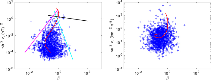
Figure 6. Left: comparison of the theoretical and observed fluctuating magnetic energy as a function of thermal plasma beta. Right: comparison of the theoretical and observed fluctuating kinetic energy as a function of thermal plasma beta. The solid red curves correspond to the theoretical results. The solid magenta line corresponds to  (Equation (15)) and the cyan line corresponds to
  (Equation (14)). The black line shows
  , the physical relevance of which is discussed below.
Download figure:
Standard image High-resolution imageFigure 6 (right) compares the theoretical (and observed)  as a function of the theoretical (and observed) plasma β. The same color and curve convention is followed. The multivalued solid red curve
  passes through the center of the observed values, which is consistent with observations. Taken together with Figure (6) (left) and Figure 5, we would conclude that the turbulent-transport model predictions of
  are reasonably consistent with the observations, despite exhibiting greater scatter.
6. Discussion and Conclusions
A very general system of coupled turbulence transport equations has been solved numerically from 1 to 75 au, and the solutions have been compared to Voyager 2 observations. The comparison yields good agreement between theory and observations. The turbulence transport model Equations (1)–(8) are 1D steady-state models obtained by assuming constant solar wind speed. However, in reality the solar wind is not so simple. Extending our 1D steady-state model to a 3D time-dependent model is therefore interesting and important if we are to understand the latitudinal and longitudinal dependence of heliospheric turbulence (Shiota et al. 2017). In doing so, the comparison of the theoretical results with the Voyager 2 measurements will be more reasonable than the 1D results because Voyager 2's latitude has changed significantly ( ) in the course of its mission. However, the 1D results are useful for understanding the transport of turbulence in the heliosphere. The coupled turbulence transport Equations (1)–(8) describe the transport of energy in forward and backward propagating modes, the residual energy, and the corresponding correlation functions for the 2D and slab cases. These transport equations were developed on the basis of an NI theory. Equations (1)–(4) describe the majority 2D core model, and (5)–(8) describe the minority slab model. An important difference between the 2D and NI model equations is the absence of the Alfvén velocity in the 2D transport equations, and its presence in the NI model equations. Thus, the 2D core model equations are completely 2D in that the fluctuations are in a plane orthogonal to the direction of the magnetic field. It is important to note that the 2D components are advected only by the large-scale solar wind flow, whereas the slab components are both advected by solar wind flow and propagate with the Alfvén velocity.
In this work, the observed turbulence values were calculated with respect to the T-component of the magnetic field. We chose the R and N component solar wind velocity and magnetic field, the solar wind density, and the solar wind temperature, and calculated various turbulence quantities from 1977 through 2004. We assumed that the calculated observed fluctuations of the R and N component solar wind velocity and magnetic field correspond to a plane orthogonal to the direction to the magnetic field. The calculated observed quantities may represent a superposition of both 2D and slab values. Finding a wavevector  would help us to calculate 2D and slab turbulence quantities. Bellan (2012, 2016) have discussed the evaluation of a wavevector
  from a single spacecraft measurement. However, since Voyager 2 does not measure the electric field
  or current
  , finding
  is not possible. Zank et al. (2017) presented a very preliminary comparison of theoretical solutions to the turbulence transport Equations (1)–(11) with observations, based on prior observations (Adhikari et al. 2015a, 2015b). Here, we studied the model equations in great detail, focusing on relating the theoretical results to the observed values. In addition, we compared the theoretical and observed density variance, the solar wind temperature, the correlation lengths corresponding to forward and backward propagating modes, residual energy, velocity variance, magnetic field variance, and the cross-correlation between the covariance of the velocity and magnetic field fluctuations as functions of heliocentric distance. We list our findings as follows.
- (1)The 2D and slab turbulent intensities such as the energy in forward and backward propagating modes, the total turbulent energy, the fluctuating kinetic and the magnetic energy are calculated as a function of heliocentric distance. The 2D energies are dominant in comparison to the slab energies throughout the heliosphere.
- (2)The 2D (
 , )/slab (, ) energies decrease with increasing heliocentric distance within ∼3–4 au), and flatten/increase in the outer heliosphere. The slab energies decrease more rapidly in comparison to the 2D energies within 3–4 au. However, the slab energies increase, and the 2D energies flatten in the outer heliosphere. We find that the theoretical varies approximately as and from 1 to ∼10 au and from ∼10 to 75 au, respectively. Similarly, varies as and , and as and within and beyond 10 au, respectively. It indicates that the energy in forward propagating modes decreases more rapidly than the energy in backward propagating modes within ∼10 au. However, both energies are approximately the same and flatten in similar fashion in the outer heliosphere.
 - (3)The 2D normalized residual energy decreases faster than the slab normalized residual energy with increasing heliocentric distance. For both normalized residual energies, the fluctuations are dominated by the fluctuating magnetic energy within ∼3–4 au, and are in approximate equipartition in the outer heliosphere. The 2D normalized residual energy is more strongly dominated by the fluctuating magnetic energy than is the slab normalized residual energy throughout the heliosphere.
- (4)The fluctuating slab kinetic and magnetic energy decrease faster than the 2D fluctuating kinetic and magnetic energy within ∼3–4 au. The fluctuating slab kinetic energy begins to increase beyond ∼4 au, whereas the 2D fluctuating kinetic energy decreases until ∼10 au, and then increases. The theoretical behaves approximately as within ∼10 au, and increases approximately as beyond ∼10 au. Similarly, varies as and from 1 to ∼10 au, and from ∼10 to 75 au, respectively, indicating that decreases more slowly in the outer heliosphere than within ∼10 au.
- (5)The correlation lengths corresponding to magnetic field fluctuations and the cross-correlation between velocity and magnetic field fluctuations increase slowly with increasing heliocentric distance. The correlation length corresponding to the velocity fluctuations decreases in the outer heliosphere, which may be due to the increase in the in the outer heliosphere.
- (6)The variance in the density fluctuations decreases with increasing heliocentric distance. The density variance varies approximately as within ∼10 au and beyond ∼10 au. In response to adiabatic expansion and in the absence of mixing associated with velocity fluctuations, the density variance decays as . However, in the presence of mixing, the density variance decreases faster than . In the outer heliosphere, the density variance flattens or decreases more slowly due to the presence of pickup ions.
- (7)The theoretical solar wind temperature exhibits similar trends to that of the observed solar wind temperature. The temperature profile is obtained by including all the nonlinear dissipation terms associated with forward and backward propagating modes and the residual energy for both 2D and slab cases. The solar wind temperature decreases approximately as from 1 to 10 au and increases approximately as beyond 10 au.
- (8)The thermal plasma beta β increases from 1 to ∼2 au, and then decreases up to ∼20 au, after which it increases beyond ∼20 au with increasing heliocentric distance. The plasma β is smaller than 1 beyond ∼3 au, although it would be larger than 1 if the pickup ion pressure were included. The magnetic field fluctuation variance is a multivalued function of plasma beta exhibiting good agreement with the distribution of the observed. Although bounded by curves corresponding to an adiabatic temperature profile, it is clear that a turbulent transport model best captures the relationship for . We note too that the relationship suggested by Squire et al. (2016) (and also Bale et al. 2016) to bound as a function of β does not appear to be validated observationally beyond 1 au, possibly because the thermal plasma beta is O(1) or less. The predicted curve, also multivalued, clearly splits the observed distribution of but the spread is large. If taken together with the predicted and observed , the predicted and observed is consistent with a turbulence transport model.


Based on the Zank et al. (2017) model, we find that the predicted variances  ,
,  ,
,  , the Elsässer energies
  , ET, and the temperature T, match the observed quantities surprisingly well given the simplicity of the model and the extended time and distance over which the observations were taken. Some of the derived quantities,
  ,
,  , and rA, and the correlation lengths, do not compare as well to the observed values, which exhibit significant scatter. Part of the large scatter may derive from the low-resolution plasma data sets.
We acknowledge the partial support of NASA grants NNX08AJ33G, Subaward 37102-2, NNX14AC08G, NNX14AJ53G, A99132BT, RR185-447/4944336, and NNX12AB30G.
Footnotes
- 6
Note that the plasma beta is computed on the basis of the background thermal solar wind measurements only. Voyager 2 cannot measure interstellar pickup ions, which form the dominant thermal component of the solar wind (Zank 1999) beyond ∼10 au. However, the PUI plasma is not thermally equilibrated with the thermal solar wind plasma (Zank et al. 2014, 2017; Zank 2015) and the incompressible 2D and slab fluctuations are largely decoupled from the PUI component (Zank et al. 2014). The inclusion of PUIs formally makes the plasma beta
() in the outer heliosphere, but the nonequilibration of thermal and PUI plasma makes it meaningful to consider the relationship of different variances with respect to the thermal solar wind plasma β (Zank et al. 2014).

