


Abstract
We present the analysis of the binary gravitational microlensing event MOA-2015-BLG-020. The event has a fairly long timescale (∼63 days) and thus the light curve deviates significantly from the lensing model that is based on the rectilinear lens-source relative motion. This enables us to measure the microlensing parallax through the annual parallax effect. The microlensing parallax parameters constrained by the ground-based data are confirmed by the Spitzer observations through the satellite parallax method. By additionally measuring the angular Einstein radius from the analysis of the resolved caustic crossing, the physical parameters of the lens are determined. It is found that the binary lens is composed of two dwarf stars with masses  and
and  in the Galactic disk. Assuming that the source star is at the same distance as the bulge red clump stars, we find the lens is at a distance
  . We also provide a summary and short discussion of all of the published microlensing events in which the annual parallax effect is confirmed by other independent observations.
Export citation and abstract BibTeX RIS
1. Introduction
In a microlensing event, companions to the primary lens object can be detected via their perturbations to the single-lens light curve (Mao & Paczynski 1991; Gould & Loeb 1992). From such perturbations, dimensionless parameters can be derived that are related to the binary system, such as the binary mass ratio q and the projected separation s (Gaudi & Gould 1997). Here, s is the instantaneous angular separation between the two components normalized to the angular Einstein radius

where  is the total lens mass, and
Here,  is the lens-source relative parallax, and
  and
and  are the distances to the lens and the source, respectively.
Although statistical conclusions can be drawn from measurements of q and s, the physical properties of the lens system, such as  , are of more interest. By far, the most popular way to convert from microlensing observables to physical quantities is to combine the measurements of
  and the microlensing parallax,
  . Then,

There are several ways to measure  (see a short summary given in Zhu et al. 2015), but the most common is to use the finite-source effect, which is the deviation in the light curve from the point-like source model due to the extended nature of the source star (Yoo et al. 2004).
For most published binary events, the microlensing parallax parameter  is measured through the annual parallax effect, in which Earth's acceleration around the Sun introduces deviations from rectilinear motion in the lens-source relative motion (Gould 1992). This method generically assumes that the lens (or lens system) and the source (or source system) are, or can be treated as, not undergoing acceleration. For binary lens events, each component is under acceleration by the other, and this so-called lens orbital motion effect can be confused with the annual parallax effect (Batista et al. 2011).
Therefore, it is important to understand the validity of the annual parallax method for binary-lens events in practical use. This can be done by observing the binary system after the event, either photometrically (Dong et al. 2009; Bennett et al. 2010) or spectroscopically (Boisse et al. 2015; Yee et al. 2016). Another way is to measure  via the satellite parallax method (Refsdal 1966; Gould 1994). This is done by observing the same microlensing event from at least two well-separated locations; the difference between the light curves from these locations informs the parameter
  . The microlensing parallax measured in this way is then determined independently from the orbital motion effect, and thus can be used to test the annual parallax method.
The Spitzer microlensing campaigns utilize the Spitzer Space Telescope to measure  via the satellite parallax method for hundreds of microlensing events (e.g., Calchi Novati et al. 2015a; Udalski et al. 2015; Yee et al. 2015a; Zhu et al. 2015). Of the several published binary events, OGLE-2015-BLG-0479, is found to have inconsistent
  from the annual parallax and satellite parallax methods, and this inconsistency can be well explained by the full orbital motion of the lens system (Han et al. 2016). In the case of OGLE-2015-BLG-0196 and OGLE-2016-BLG-0168, the annual parallax effect is confirmed by the satellite parallax method (Han et al. 2017; Shin et al. 2017).
In this paper, we present the analysis of Spitzer binary event MOA-2015-BLG-020. This is the second published case in which the annual parallax effect agrees with the satellite parallax effect. We summarize the ground-based and space-based observations in Section 2, describe the light curve modeling in Section 3, and derive the physical properties of the binary system in Section 4. In Section 5, we review all of the published microlensing binaries in which the annual parallax effect has been confirmed or contradicted by other methods, and discuss the implications.
2. Observations
2.1. Ground-based Alert and Follow-up
At UT 10:06 on 2015 February 16 ( ), the MOA collaboration identified the microlensing event MOA-2015-BLG-020 at equatorial coordinates (R.A., decl.)2000 = (17h52m52
 78, −32°29'09
 1), with corresponding Galactic coordinates (l, b)2000 = (−2
 24, −316), based on data taken by its 1.8 m telescope with a 2.2 deg2 field at Mt. John, New Zealand. These MOA observations were taken in a broad ∼R+I bandpass at 15-minute cadence. The OGLE collaboration independently discovered this event about 2.5 days after the MOA alert. It was alerted as OGLE-2015-BLG-0102 through the OGLE Early Warning System (Udalski et al. 1994; Udalski 2003), based on observations from the 1.4 deg2 camera on its 1.3 m Warsaw Telescope at the Las Campanas Observatory in Chile. This microlensing event lies in the OGLE-IV field BLG535 (Udalski et al. 2015), meaning that it received OGLE observations at a cadence of 2–3 observations per night.
Event MOA-2015-BLG-020 also lies in one of the four prime fields of the Korean Microlensing Telescope Network (KMTNet; Kim et al. 2016), and thus received dense coverage from KMTNet. In 2015, KMTNet observed a ∼16 deg2 prime microlensing field at ∼10-minute cadence when the bulge was visible. The KMTNet consists of three 1.6 m telescopes, each equipped with a 4 deg2 field of view camera. The observations started on 2015 February 3 (HJD' = 7056.9) for its CTIO telescope, 2015 February 19 (HJD' = 7072.6) for its SAAO telescope, and 2015 June 9 (HJD' = 7182.9) for its SSO telescope, respectively.
This event was also observed by the Las Cumbres Observatory Network (LCO; Brown et al. 2013) to support the 2015 Spitzer microlensing campaign; see Street et al. (2016) for a more detailed description of the LCO observations. Between HJD' = 7123.7 and 7174.8, event MOA-2015-BLG-020 received in total 186 observations from two 1 m telescopes at CTIO, 105 observations from two 1 m telescopes at SAAO, and 76 observations from two 1 m telescopes at SSO.
All ground-based data were reduced using the standard or variant version of the image subtraction method developed by Alard & Lupton (1998), employing a spatially variant kernel as necessary (see also Bramich 2008).
2.2. Spitzer Follow-up
Event MOA-2015-BLG-020 was selected for Spitzer IRAC 3.6 μm observations as part of the 2015 Spitzer microlensing campaign to probe the Galactic distribution of planets (Calchi Novati et al. 2015a; Zhu et al. 2017). The general description of the campaign and the target selection protocol can be found in Udalski et al. (2015) and Yee et al. (2015b), respectively. By the time the 2015 Spitzer program had started,45 the binary nature of the current event had already been established. Therefore, it was selected as a "subjective binary" on 2015 June 1 (HJD = 2457175), meaning that Spitzer observations were taken specifically for the purpose of measuring the mass of the binary. Then observations started on 2015 June 8 (HJD = 2457182) and ended on 2015 July 15 (HJD = 2457219), when this target moved out of Spitzer's Sun-angle window. The cadences were determined objectively, and in total 61 observations were taken.
The Spitzer data were reduced by the software that was designed specifically for this microlensing program (Calchi Novati et al. 2015b). In the present case, because the source star is very bright and red, it was saturated on the Spitzer images that were taken in the first few days. Although the saturation issue is in principle solvable (e.g., OGLE-2015-BLG-0763; Zhu et al. 2016), we decided to exclude the first 10 data points that are potentially affected by saturation, on the basis that no particularly interesting behavior occurred during this time interval. In the end, we include 51 Spitzer observations spanning from HJD' = 7185.7 to 7221.8 for the parallax measurement.
3. Light Curve Modeling
3.1. Initial Solution Search
The light curve of event MOA-2015-BLG-020 suggests that it is a typical binary microlensing event (see Figure 1). In the standard terminology (i.e., binary event without parallax and lens orbital motion effects), the following seven parameters are used for characterizing a binary light curve: the time of the closest approach between the source and the binary lens (gravitational) center, t0; the impact parameter normalized by the Einstein radius, u0; the event timescale,  the source size normalized by the Einstein radius, ρ; the projected separation between the binary components normalized to the Einstein radius, s; the binary mass ratio, q; and the angle between the binary-lens axis and the lens-source relative motion, α. There are two further flux parameters that describe the source flux
  and the blending flux
  for each observatory j that translate the magnification A to the observed flux at given time ti

These flux parameters are found for each data set using linear fit. We use the the advanced contour integration code, VBBinaryLensing,46
to compute of the binary lens magnification  . This code includes a parabolic correction in Green's line integral, and can automatically adjust the step size of the integration based on the distance to the binary caustic, in order to achieve a desired precision in magnification. See Bozza (2010) for more details.
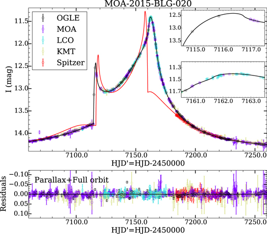
Figure 1. Light curve of event MOA-2015-BLG-020. In the top panel, the blue and red lines are the best-fit theoretical light curves for ground-based and satellite observations. The bottom panel shows the residual from the best model. Data points from different collaborations are shown with different colors. The data used to create this figure are available.
Download figure:
Standard image High-resolution imageWe start with a grid search on the ground-based data alone for the possible binary solution (or solutions). The grid search is conducted on parameters (log s, log q, log ρ, α), with 16 values equally spaced between −1 ≤ log s ≤ 1, −3 ≤ log q ≤ 0, −4 ≤ log ρ ≤ 0, and 0° ≤ α ≤ 360°, respectively. For each set of (log s, log q, log ρ, α), we find the minimum  by going downhill on the remaining parameters
  .
.
The global minimum is found at log s ∼ 0 (s ∼ 1), log q ∼ −0.6 (q ∼ 0.25), log ρ ∼ 2, and α ∼ 220°, and there is no other locus on this grid that has similar  .
.
We then refine the solution by performing Markov Chain Monte Carlo (MCMC) analysis around the initial solution found by the previous grid search, which employs the emcee ensemble sampler (Foreman-Mackey et al. 2013).
3.2. Inclusion of Microlensing Parallax Effect
The microlensing parallax effect has to be taken into account in order to simultaneously model the ground-based and space-based data. This effect invokes two additional parameters,  and
and  , which are the northern and eastern components of the parallax vector
  .
.
We try to constrain  based on ground data alone, and by simultaneously modeling ground and Spitzer data, in order to check the consistency between annual parallax and satellite parallax effects. This check is possible here because MOA-2015-BLG-020 occurred relatively early in the season and had a fairly long timescale.
The annual parallax effect leads to two discrete solutions arising from the ±u0 degeneracy (e.g., Smith et al. 2003; Poindexter et al. 2005). In the case of MOA-2015-BLG-020, we find that the two solutions have  because of strong annual parallax effect, indicating that the
  solution is strongly favored over the
  solution. We show in Figure 2 the 3-σ constraints on
  based on ground-based data alone.

Figure 2. Distribution of microlensing parallax parameters  and
and  in the east and north directions. The red and blue contours are obtained based on the combined ground+Spitzer data and the ground data alone, respectively. The three contours show 1-σ (
 ), 2-σ (
 ), and 3-σ (
 ) confidence regions of the full orbit model.
Download figure:
Standard image High-resolution imageWe then take into account the satellite parallax effect in order to include Spitzer data. We extract the geocentric locations of Spitzer during the entire season from the JPL Horizons website,47
and project them onto the observer plane. The projected locations are then oriented and rescaled according to a given  to work out Spitzer's view of the microlensing geometry.
We include the ![$I-[3.6\,\mu {\rm{m}}]$](https://content.cld.iop.org/journals/0004-637X/845/2/129/revision1/apjaa813bieqn39.gif) color constraint on the source star to better constrain the parallax parameters, considering the simple monotonic falling behavior of the Spitzer light curve. This has been demonstrated to be effective in single-lens cases (e.g., Calchi Novati et al. 2015a; Zhu et al. 2017). The
color constraint on the source star to better constrain the parallax parameters, considering the simple monotonic falling behavior of the Spitzer light curve. This has been demonstrated to be effective in single-lens cases (e.g., Calchi Novati et al. 2015a; Zhu et al. 2017). The ![$I-[3.6\,\mu {\rm{m}}]$](https://content.cld.iop.org/journals/0004-637X/845/2/129/revision1/apjaa813bieqn40.gif) color constraint comes from putting the measured V − I source color into the
color constraint comes from putting the measured V − I source color into the ![$I-[3.6\,\mu {\rm{m}}]$](https://content.cld.iop.org/journals/0004-637X/845/2/129/revision1/apjaa813bieqn41.gif) versus V − I relation, which is derived based on a nearby field stars of similar colors (see Calchi Novati et al. 2015b for more details). This yields
versus V − I relation, which is derived based on a nearby field stars of similar colors (see Calchi Novati et al. 2015b for more details). This yields ![$I-[3.6\,\mu {\rm{m}}]=3.18\pm 0.05$](https://content.cld.iop.org/journals/0004-637X/845/2/129/revision1/apjaa813bieqn42.gif) mag. During the MCMC process, we calculate
mag. During the MCMC process, we calculate ![$I-[3.6\,\mu {\rm{m}}]$](https://content.cld.iop.org/journals/0004-637X/845/2/129/revision1/apjaa813bieqn43.gif) from the flux parameters (which are found using a linear fit), and reject any values that are
from the flux parameters (which are found using a linear fit), and reject any values that are  away from the central value.
The constraints on  from the simultaneous modeling of ground and Spitzer data are also shown in Figure 2. We note that these are the constraints from annual parallax and satellite parallax signals together. In order to separate constraints from these two types of parallaxes, we assume that the posteriors of the ground-only and ground+Spitzer fits are multivariate Gaussians, and derive the covariance matrix of the satellite parallax part (see the Appendix and Gould 2003) The derived matrix has a determinant that is statistically consistent with zero, which indicates a strong correlation between
  and
and  . This is because the Spitzer observations occasionally only measure a one-dimensional parallax component (see Shvartzvald et al. 2015 for a detailed discussion). We nevertheless proceed with the standard procedure and compute the difference between the annual parallax and the satellite parallax measurements, and find
  . Although this would formally indicate a probability of
  , it is actually well within the systematic uncertainty that the ground-based data can introduce.48
Therefore, the small
, it is actually well within the systematic uncertainty that the ground-based data can introduce.48
Therefore, the small  indicates a good agreement between the annual parallax and the satellite parallax.
Notice that we took into account the four-fold parallax degeneracy (often denoted as (++), (+,−), (−,+), and (−,−)). Two of these are eliminated since the  solution is excluded by the ground-based data, while the (+,−) degeneracy from Spitzer is also eliminated.
3.3. Inclusion of Binary Lens Orbital Motion Effect
We then introduce the lens orbital motion effect into the light curve modeling. Despite the degeneracy between orbital motion and parallax, as we will see below, in this case this has no effect on the measured values or uncertainties of the parallax. We introduce orbital motion into the models in two different ways. First, we use the linear orbital motion approximation, which involves two parameters,  and
and  . For the binary system to remain bound, we also impose the constraints on the projected kinetic to potential energy ratio (Dong et al. 2009). Second, we also include z and
  in addition to
  and
and  , in order to account for the full Keplerian motion of the binary system. Here z and
  quantify the binary separation (normalized to the Einstein radius) along the line of sight and its time derivative, respectively. See Skowron et al. (2011) for the conversion between these phase-space parameters and Keplerian parameters. This conversion requires an input of the source angular size
  in order to set the absolute physical scale, and we use
  (see Section 4). Once the Keplerian parameters are derived, we check the orbital period P and reject any solution with
  , in order to avoid the influence of systematics in the data.

Figure 3. Triangle plot of the full orbit model with both ground-based and space-based data included in the fit. The orbital parameters (especially z) are not constrained as well as the standard microlensing parameters. Notice that the bimodal distribution of  is caused by excluding samples with a very long period (millions of years). Without such an exclusion, there would be only one peak.
Download figure:
Standard image High-resolution imageThe results of two modelings with different treatment of the orbital motion are given in Table 1; the triangle diagram of the fitting parameters for the full orbital model is shown in Figure 3. The source trajectories and caustics of the full orbit motion are shown in Figure 4. This solution has slightly worse  than the linear orbital motion solution, even though the former has two more free parameters. This is because the linear orbit solution (with the ratio of the perpendicular kinetic energy to the potential energy,
  ) has preferentially long orbital periods (
 years) for the binary system, which are not allowed in the full orbit solution. Nevertheless, the microlensing parameters (especially the microlens parallax) are stable regardless of whether and how the lens orbital motion is included.
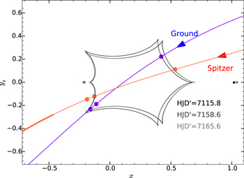
Figure 4. Caustics patterns for the event MOA-2015-BLG-020. Three caustic curves are shown for three different epochs (caustic entrance from the ground, caustic exits from Spitzer and ground), although the two at HJD' = 7158.6 and 7165.6 almost overlap. The corresponding lens and source positions are shown as solid dots. The source trajectories for the ground and Spitzer are shown as blue and red curves, respectively. The arrows indicate the directions of the source motions. The bold line segment indicates the epochs of the Spitzer data.
Download figure:
Standard image High-resolution imageTable 1. Best-fit Parameters
| Parametersa | Ground+Spitzer | Ground-only | |||||
|---|---|---|---|---|---|---|---|
| Full Orbit | Linear Orbit | Parallax Only | Full Orbit | Linear Orbit | Parallax Only | Without Parallax | |
 dof dof |
4003.5/4028 | 4000.8/4030 | 4222.4/4032 | 3940.1/3967 | 3936.4/3969 | 4162.0/3971 | 5907.2/3973 |

|
0.0962 ± 0.0003 | 0.0963 ± 0.0003 | 0.0940 ± 0.0002 | 0.0962 ± 0.0003 | 0.0963 ± 0.0003 | 0.0940 ± 0.0002 | 0.08767 ± 0.00009 |

|
−0.684 ± 0.002 | −0.683 ± 0.002 | −0.703 ± 0.001 | −0.685 ± 0.002 | −0.685 ± 0.002 | −0.703 ± 0.001 | −0.7477 ± 0.0007 |
| u0 | 0.0716 ± 0.0008 | 0.0715 ± 0.0008 | 0.0798 ± 0.0004 | 0.0711 ± 0.0008 | 0.0715 ± 0.0008 | 0.0799 ± 0.0004 | 0.09109 ± 0.00015 |
| t0 | 7145.48 ± 0.03 | 7145.46 ± 0.03 | 7145.72 ± 0.03 | 7145.48 ± 0.03 | 7145.51 ± 0.03 | 7145.71 ± 0.03 | 7145.66 ± 0.01 |
| tE (days) | 63.56 ± 0.06 | 63.55 ± 0.06 | 62.94 ± 0.06 | 63.74 ± 0.07 | 63.61 ± 0.08 | 62.94 ± 0.06 | 64.69 ± 0.03 |

|
−1.745 ± 0.002 | −1.744 ± 0.002 | −1.757 ± 0.002 | −1.746 ± 0.002 | −1.745 ± 0.002 | −1.757 ± 0.002 | −1.7969 ± 0.0009 |
| α (deg) | 219.12 ± 0.08 | 219.14 ± 0.08 | 218.27 ± 0.05 | 219.18 ± 0.08 | 219.14 ± 0.09 | 218.28 ± 0.05 | 217.43 ± 0.03 |

|
−0.223 ± 0.004 | −0.223 ± 0.005 | −0.220 ± 0.006 | −0.212 ± 0.006 | −0.211 ± 0.010 | −0.218 ± 0.006 | ⋯ |

|
−0.007 ± 0.002 | −0.006 ± 0.002 | 0.003 ± 0.002 | −0.010 ± 0.002 | −0.010 ± 0.002 | 0.003 ± 0.002 | ⋯ |
 (year−1) (year−1) |
0.212 ± 0.015 | 0.217 ± 0.017 | ⋯ | 0.240 ± 0.017 | 0.225 ± 0.018 | ⋯ | ⋯ |
 (rad/year) (rad/year) |
0.383 ± 0.014 | −1.197 ± 0.038 | ⋯ | 0.371 ± 0.017 | −1.197 ± 0.040 | ⋯ | ⋯ |
| z | 7.03 ± 3.17 | ⋯ | ⋯ | 4.78 ± 4.52 | ⋯ | ⋯ | ⋯ |
 (year−1) (year−1) |
0.037 ± 0.258 | ⋯ | ⋯ | 0.277 ± 0.270 | ⋯ | ⋯ | ⋯ |
| V − I | 2.875 ± 0.003 | 2.874 ± 0.003 | 2.867 ± 0.003 | 2.876 ± 0.003 | 2.874 ± 0.003 | 2.868 ± 0.002 | 2.860 ± 0.002 |
Note.
aWe use in our full orbit model.
Download table as: ASCIITypeset image
4. Physical Parameters
We estimate the angular size of the source following the standard procedure (Yoo et al. 2004). First, we measure the centroid of the red clump in the OGLE  color–magnitude diagram (CMD) of the stars within 2' × 2' of our event (see Figure 5). By using stars in the box
  and
and  , we find the centroid of the red clump to be (V − I, I)RC = (2.11 ± 0.05, 16.05 ± 0.11). This, when combined with the instrumental color and magnitude of the source star (V − I, I)S,OGLE = (2.87, 14.34), yields an offset of Δ(V − I, I)OGLE = (V − I, I)S,OGLE − (V − I, I)RC,OGLE = (0.76, −1.71). After applying the correction of the non-standard V band of OGLE-IV (Udalski et al. 2015; Zhu et al. 2015) Δ(V − I)JC = Δ(V − I)OGLE × 0.92 = 0.70 (in which "JC" represents the standard Johnson-Cousins system) and adapting the intrinsic color and magnitude of the clump (V − I, I)RC,0 = (1.06, 14.56) (Bensby et al. 2013; Nataf et al. 2013), we find that the intrinsic color and magnitude of source is (V − I, I)S,0 = Δ(V − I, I)JC + (V − I, I)RC,0 = (1.76, 12.85).
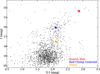
Figure 5. OGLE-IV calibrated color–magnitude diagram of the stars (black dots) within 2' × 2' of MOA-2015-BLG-020/OGLE-2015-BLG-0102. The blue dot shows the centroid of the red clump stars. The red asterisk indicates the position of the microlensed source, and the yellow triangle shows the position of the blended object.
Download figure:
Standard image High-resolution imageTo determine the source angular size, we employ the color-surface brightness relation of giant stars from Kervella et al. (2004), and finally find

Therefore,

Then we obtain the total mass of the system using Equation (3):

Combined with the mass ratio from our fit, we find that the lens system is a binary of  and
and  . The lens-source relative parallax is
  , indicating a disk binary. Under the assumption that the source is at the same distance as the red clump centroid at this location (
 , Nataf et al. 2013), the distance to the lens is

The lensing binary is vertically about 120 pc away from the Galactic plane, likely from the thin disk.
The binary components are separated in projection by

We summarize the physical parameters in Table 2.
Table 2. Physical Parameters of the Binary Lens System MOA-2015-BLG-020
| Parameters | |
|---|---|
 (mas) (mas) |
1.329 ± 0.049 |
 (mas) (mas) |
0.296 ± 0.017 |
M1 ( ) ) |
0.606 ± 0.028 |
M2 ( ) ) |
0.125 ± 0.006 |
| Distance to lens (kpc) | 2.44 ± 0.10 |
| Projected separation (au) | 4.04 ± 0.23 |
Geocentric proper motion (mas  ) ) |
7.64 ± 0.28 |
Download table as: ASCIITypeset image
5. Discussion
We analyzed the binary-lensing event MOA-2015-BLG-020, which was observed both from the ground and from the Spitzer Space Telescope. The light curve from ground-based observations significantly deviated from the lensing model based on the rectilinear lens-source relative motion, and we measured the microlensing parallax from the analysis of the deviation. The measured parallax was confirmed by the Spitzer data, showing the consistency between annual parallax and satellite parallax effects. By additionally measuring the angular Einstein radius from the analysis of the resolved caustic crossing, the mass and distance to the lens are determined. We find that the lens is a binary composed of two low-mass stars located in the Galactic disk. In our analysis, we find that the linear orbit model and full orbit model can fit the data almost equally well. Although the full orbit parameters z and  are not well constrained, we report lens physical parameters based on the full orbit model because of its physical foundation (Han et al. 2016).
The binary-lensing event MOA-2015-BLG-020 is peculiar in one aspect. Usually, the light curve for a caustic-crossing binary event has one sharp rise and one sharp fall during the caustic entrance and exit, respectively, producing a "U"-shaped light curve. However, for this binary event, the caustic exit gracefully merges with the cusp crossing (see Figure 4), which causes the absence of the sharp decline in the ground-based light curve. This is almost a direct result of lens orbital motion. Note that this sharp decline is predicted to be present in the space-based light curve, but it is not observable by Spitzer due to various observational constraints (see Udalski et al. 2015 for details).
In Table 3, we summarize the published microlensing binaries in which the parallax parameters detected from ground (through annual parallax effect) are tested by other methods. The parallax parameters based on ground data in OGLE-2011-BLG-0417 and OGLE-2015-BLG-0479 seem to be inconsistent with the results of independent checks. Although there is still the possibility that the parallax detected by microlensing is wrong, it is believed that the radial velocity measurements for OGLE-2011-BLG-0417 do not test the parallax model. The reason is that the blended light of OGLE-2011-BLG-0417 is not the lens because it is brighter than predicted flux from the lens. The inconsistency in OGLE-2015-BLG-0479 is expected because of the strong lens orbital motion effect. Indeed, it is because of this inconsistency that the full Keplerian parameters of the binary in OGLE-2015-BLG-0479 can be well constrained (Han et al. 2016).
Table 3. Summary of Events that have Annual Parallax Tested by Other Measurements
| Event Name | Confirmed? | ( , ,  ) ) |
Mass Ratio(s) |
 (day) (day) |
t0(HJD') | u0 |

|

|

|
References |
|---|---|---|---|---|---|---|---|---|---|---|
| High-resolution Imaging | ||||||||||
| OGLE-2005-BLG-071 | Yes | ( , -0.26 ± 0.05) , -0.26 ± 0.05) |

|
71.1 | 3480.7 (04/20) | 0.0282 | 19.5 |

|
⋯ | 1, 2 |
| OGLE-2006-BLG-109 | Yes | (−0.316 ± 0.013, 0.139 ± 0.006) |

|
128.1 | 3831.0 (04/05) | 0.00345 | 20.9 | 13.5 | ⋯ | 3, 4 |
| OGLE-2007-BLG-349 | Yes | 0.204 ± 0.034a |
|
118 | 4348.7 (09/05) | −0.00198 | 20.4 | 153 | ⋯ | 5 |
| Radial Velocity: | ||||||||||
| OGLE-2009-BLG-020 | Yes | (−0.022 ± 0.086, 0.149 ± 0.010) | 0.273 | 76.9 | 4917.3 (03/26) | 0.0613 | 16.4 | ⋯ | 26.3 | 6, 7 |
| OGLE-2011-BLG-0417 | No | (0.375 ± 0.015, −0.133 ± 0.003) | 0.292 | 92.3 | 5813.3 (09/08) | −0.0992 | ⋯ | 2024 | 656 | 8, 9, 10 |
| Satellite Parallax:b | ||||||||||
| OGLE-2014-BLG-0124 | Yes | (0.018 ± 0.012, 0.108 ± 0.023) |

|
131 | 6836.2 (06/27) | 0.2099 | 18.6 | ⋯ | ⋯ | 11 |
| OGLE-2015-BLG-0479c | Nod | (−0.06 ± 0.01, −0.11 ± 0.01) | 0.81 | 86.3 | 7166.4 (05/23) | 0.417 | 19.6 | ⋯ | 43.5 | 12 |
| OGLE-2015-BLG-0196 | Yes | (0.198 ± 0.016, 0.100 ± 0.009) | 0.99 | 96.7 | 7115.5 (04/03) | −0.037 | 15.9 | 2527.6 | 24.4 | 13 |
| OGLE-2016-BLG-0168 | Yes | (0.382 ± 0.022,0.057 ± 0.011) | 0724 | 97.0 | 7492.5 (04/13) | −0.201 | 19.5 | 159.4 | 115.04 | 14 |
| MOA-2015-BLG-020 | Yes | (−0.223 ± 0.005, −0.007 ± 0.002) | 0.207 | 63.6 | 7145.5 (05/03) | 0.0716 | 14.3 | 1983.5 | 218.9 | This work |
Notes.
aBennett et al. (2016) used a different parameterization, with which the amplitude of the parallax vector was constrained. bThe microlens parameters are all from ground-based detection unless otherwise stated. The color, magnitude, and are from the combination of ground and satellite data sets.
cParameters of OGLE-2015-BLG-0479 are from the analysis of the combination data set.
dThat the full orbital motion is detectable in this event is noticeable based purely on the ground-based data. Therefore, this inconsistency is expected.
are from the combination of ground and satellite data sets.
cParameters of OGLE-2015-BLG-0479 are from the analysis of the combination data set.
dThat the full orbital motion is detectable in this event is noticeable based purely on the ground-based data. Therefore, this inconsistency is expected.
References. 1. Udalski et al. (2005), 2. Dong et al. (2009), 3. Gaudi et al. (2008), 4. Bennett et al. (2010), 5. Bennett et al. (2016), 6. Skowron et al. (2011), 7. Yee et al. (2016), 8. Shin et al. (2012), 9. Boisse et al. (2015), 10. Santerne et al. (2016), 11. Udalski et al. (2015), 12. Han et al. (2016), 13. Han et al. (2017), 14. Shin et al. (2017).
Download table as: ASCIITypeset image
For the remaining events, the microlensing parallax parameters from the annual parallax effect are confirmed by additional observations (high-resolution imaging, radial velocity, or satellite parallax). As expected, they all have relatively long timescales ( days), and the majority of them peaked (as seen from ground) either early (before May) or late (after August) in the microlensing season. Among these events, half are confirmed by ground observations (adaptive optics or radial velocity) and they all have a small impact parameter u0, while those confirmed by satellite observations could have larger u0 (modest magnification). This highlights Spitzer's power to discover parallax events for moderately magnified events. The abundance of stellar binaries with
  is roughly uniform as a function of
  (
( ), consistent with Trimble (1990), although we caution that the number of events is small and no selection effects have been taken into account. As more and more lenses with definite masses are determined from microlensing, it will be very interesting to study these statistics much more carefully in the future.
This work has been supported in part by the National Natural Science Foundation of China (NSFC) grants 11333003 and 11390372 (S.M.). This research uses data obtained through the Telescope Access Program (TAP), which has been funded by the Strategic Priority Research Program "The Emergence of Cosmological Structures" (grant No. XDB09000000), National Astronomical Observatories, Chinese Academy of Sciences, and the Special Fund for Astronomy from the Ministry of Finance. Work by W.Z., Y.K.J., I.G.S., and A.G. was supported by AST-1516842 from the US NSF and JPL grant 1500811. Work by J.C.Y. was performed in part under contract with the California Institute of Technology (Caltech)/Jet Propulsion Laboratory (JPL) funded by NASA through the Sagan Fellowship Program executed by the NASA Exoplanet Science Institute. This research has made use of the KMTNet system operated by the Korea Astronomy and Space Science Institute (KASI) and the data were obtained at three host sites of CTIO in Chile, SAAO in South Africa, and SSO in Australia. The OGLE Team thanks Drs. G. Pietrzyński and Ł. Wyrzykowski for their contribution to the collection of the OGLE photometric data over the past years. The OGLE project has received funding from the National Science Centre, Poland, grant MAESTRO 2014/14/A/ST9/00121 to A.U. Work by C.H. was supported by the grant (2017R1A4A1015178) of the National Research Foundation of Korea. This work makes use of observations from the LCO network, which includes three SUPAscopes owned by the University of St Andrews. The RoboNet programme was an LCO Key Project using time allocations from the University of St Andrews, LCOGT, and the University of Heidelberg together with time on the Liverpool Telescope through the Science and Technology Facilities Council (STFC), UK. This research has made use of the LCO Archive, which was operated by the California Institute of Technology, under contract with the Las Cumbres Observatory. The MOA project is supported by JSPS KAKENHI grant Nos. JSPS24253004, JSPS26247023, JSPS23340064, JSPS15H00781, and JP16H06287.
Software: corner.py (Foreman-Mackey 2016), emcee (Foreman-Mackey et al. 2013), VBBinaryLensing (Bozza 2010).
Appendix:
Let a and c denote a parallax measurement and its covariance matrix, and the subscripts "comb" and "ground" indicate quantities appropriate for the combined and ground-based data. For example,  and
and  are the measured parallax and its covariance matrix from our MCMC fits for the combined data. We follow Gould (2003) to derive the "Spitzer" parallax and the consistency between the ground and Spitzer parallaxes (expressed as
  ) through the following steps. First, we introduce several quantities for later use
Then we calculate the corresponding quantities for the Spitzer parallax
Finally, we compute the difference between the annual and satellite parallax measurements
where
Footnotes
- 45
Although Spitzer observations did not start until 2015 June 8 (HJD = 2457182), the target selections started in late 2015 May.
- 46
- 47
- 48
In other words, we would never consider it a reliable parallax measurement if the annual parallax only has
 improvement compared to the standard model.
