


Abstract
The shape of the damping profile of kink oscillations in coronal loops has recently allowed the transverse density profile of the loop to be estimated. This requires accurate measurement of the damping profile that can distinguish the Gaussian and exponential damping regimes, otherwise there are more unknowns than observables. Forward modeling of the transverse intensity profile may also be used to estimate the width of the inhomogeneous layer of a loop, providing an independent estimate of one of these unknowns. We analyze an oscillating loop for which the seismological determination of the transverse structure is inconclusive except when supplemented by additional spatial information from the transverse intensity profile. Our temporal analysis describes the motion of a coronal loop as a kink oscillation damped by resonant absorption, and our spatial analysis is based on forward modeling the transverse EUV intensity profile of the loop under the isothermal and optically thin approximations. We use Bayesian analysis and Markov chain Monte Carlo sampling to apply our spatial and temporal models both individually and simultaneously to our data and compare the results with numerical simulations. Combining the two methods allows both the inhomogeneous layer width and density contrast to be calculated, which is not possible for the same data when each method is applied individually. We demonstrate that the assumption of an exponential damping profile leads to a significantly larger error in the inferred density contrast ratio compared with a Gaussian damping profile.
Export citation and abstract BibTeX RIS
1. Introduction
Standing kink oscillations were first detected in coronal loops using the Transition Region And Coronal Explorer (TRACE; Aschwanden et al. 1999, 2002; Nakariakov et al. 1999). Their detection is now routine (e.g., Zimovets & Nakariakov 2015; Goddard et al. 2016), and thanks to the increased spatial and temporal resolution of modern instruments such as the Atmospheric Imaging Assembly (AIA; Lemen et al. 2012) of the Solar Dynamics Observatory (SDO), they have great potential for seismological investigation of the coronal plasma (e.g., reviews by De Moortel & Nakariakov 2012; Stepanov et al. 2012; Pascoe 2014; De Moortel et al. 2016). They are commonly used to infer the strength of the coronal magnetic field (e.g., Nakariakov et al. 1999; Nakariakov & Ofman 2001; Van Doorsselaere et al. 2008; White & Verwichte 2012; Pascoe et al. 2016b; Sarkar et al. 2016). Additional structuring information may be obtained using higher harmonics, which there is increasing evidence of (e.g., Verwichte et al. 2004; De Moortel & Brady 2007; Van Doorsselaere et al. 2007; Wang et al. 2008; Srivastava et al. 2013; Pascoe et al. 2016a, 2017a, 2017c; Li et al. 2017). The strong damping of kink oscillations is attributed to resonant absorption (Sedláček 1971), which requires a smooth transition between the high-density plasma inside coronal loops and the background plasma. Inside this inhomogeneous layer, energy is transferred from kink to Alfvén waves where the local Alfvén speed matches the kink speed Ck on a timescale comparable to the period of oscillation (e.g., Hollweg & Yang 1988; Goossens et al. 2002; Ruderman & Roberts 2002).
The damping rate due to resonant absorption depends on the transverse density profile of the coronal loop. The observed damping rate can therefore be used in seismological analysis of oscillations to obtain information about the transverse structuring. However, the damping rate is a single observable, whereas models for the transverse density profile are typically described by two unknowns (e.g., density contrast ratio and the width of the inhomogeneous layer). Furthermore, different models for the shape of the density profile have been considered (e.g., a sinusoidal or linear density profile inside the inhomogeneous layer), and this choice also affects the expected damping rate of kink oscillations (e.g., Goossens et al. 2002; Roberts 2008; Soler et al. 2014).
Pascoe et al. (2013) proposed a seismological method based on observing the initial Gaussian damping regime of kink oscillations in addition to the later exponential damping regime. The general damping profile (GDP) that describes these two regimes allows two observables to be measured, and hence the transverse density profile can be calculated (for the assumed density profile model). Pascoe et al. (2016b) analyzed the transverse oscillations of three coronal loops using the GDP for the first time to produce seismological inversions for the transverse density profile. This method was extended by Pascoe et al. (2017a) to describe a time-dependent period of oscillation, the presence of additional parallel harmonics, and any decayless component. Pascoe et al. (2017a) also employed a new method to account for a dynamical background trend and used Bayesian analysis to test the model against the observational data. Pascoe et al. (2017c) included an additional term in the background trend to describe loops that experience a rapid shift in the location of the equilibrium, such as the contracting loops previously analyzed by Simões et al. (2013) and Russell et al. (2015). These applications of the seismological method based on the shape of the damping profile exploit the best cases of kink oscillations that have been observed so far. However, the usefulness of seismological methods is increased by extending the number of observations to which they may be applied. In cases where the particular observational conditions are poor and less information can be reliably extracted from the oscillation data, it is necessary to fill the gap with some other source of information.
Another such source of information about the structure of coronal loops that we consider in this paper is their intensity profile. EUV imaging instruments also allow us to investigate the transverse damping profile using the observed intensity profile, for example, initial studies by Aschwanden et al. (2003, 2007) and Aschwanden & Nightingale (2005) using TRACE 171 Å. Pascoe et al. (2017b) used a similar method (applied to data from SDO/AIA) to estimate the inhomogeneous layer width of a coronal loop and found a value consistent with that calculated seismologically for the same loop in Pascoe et al. (2017a). Goddard et al. (2017) studied the density profiles of 233 coronal loops and found that the majority exhibit evidence for having an inhomogeneous layer of finite width. The potential for seismological techniques to provide structuring information is also relevant for studies of multi-threaded coronal structures considered by many authors (e.g., Lenz et al. 1999; Aschwanden et al. 2000; Pascoe et al. 2007; Brooks et al. 2012; Antolin et al. 2015; Aschwanden & Peter 2017).
In this paper, we perform a detailed analysis of a particular coronal loop, described in Section 2. The temporal (seismological) and spatial (forward modeling) diagnostic methods used are described in Section 3. In Section 4, we apply each of these methods separately to the loop data. In response to the strengths and limitations of the single-model approach, we develop techniques based on using multiple sources of data simultaneously, and the results of these multi-model methods are presented in Section 5. Further discussion of effects relevant to our method and results are in Section 6, including a comparison with numerical simulations to estimate the associated errors. Conclusions are presented in Section 7.
2. Observation
The coronal loop we analyze in this paper is shown in Figure 1. It is designated as "Event 5 Loop 1" in Goddard et al. (2016) and Pascoe et al. (2016c). In this paper, we use the seismological methods for damped kink oscillations applied in Pascoe et al. (2016b, 2017a) and the method of forward modeling the EUV intensity profile from Pascoe et al. (2017b). We apply these methods to estimate model parameters, in particular  = l/R, which is the size of the transverse inhomogeneous layer l normalized by the loop minor radius R. For these methods, we require the time series for the position of the loop and the intensity profile perpendicular to the loop axis. In our case, both of these observations are generated from the same slit (blue line in Figure 1) using the same bandpass (171 Å) of the same instrument (SDO/AIA), though this is not a requirement. A benefit of the multi-model analysis (Section 5) is its potential to combine data from different sources.
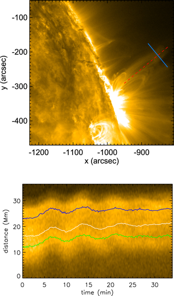
Figure 1. SDO/AIA 171 Å image (top) of the analyzed loop with its axis indicated by the dashed red line. The solid blue line shows the location of the slit used to generate the time–distance map (bottom). The white line shows the original time series used in Pascoe et al. (2016c) based on a single Gaussian fit to the intensity profile, while the green and blue lines track the two loop legs separately.
Download figure:
Standard image High-resolution imageThe bottom panel of Figure 1 shows the time–distance map for the loop starting at 04:40 on 2011 February 10, just after a B6.0 GOES-class flare that occurs at 04:39 (Zimovets & Nakariakov 2015). The white line shows the position of the loop previously used in Pascoe et al. (2016c), which was based on the assumption of a monolithic (i.e., single-thread) structure and tracked in time using the standard method of fitting each intensity profile using a Gaussian function (e.g., GAUSSFIT in IDL) and determining the loop position as the center of the Gaussian. However, on closer inspection, and by considering the orientation of the loop (top panel of Figure 1), we note that the line of sight (LOS) is almost parallel to the loop's plane, and hence the intensity profile is composed of the two legs appearing to overlap on the plane of the sky. To accurately measure the oscillation, we performed a fit using a model comprised of two structures to allow us to track each leg of the loop separately (green and blue lines in Figure 1). We note that the legs oscillate in phase with each other and with the original time series (white line), consistent with a horizontally polarized fundamental kink mode that we are viewing almost side-on.
Fitting two legs rather than a single structure also produces a lower and more accurate estimate of the loop minor radius R ≈ 7 Mm, though this is still relatively wide for a coronal loop, which facilitates the estimation of the loop density profile by forward modeling. The length of the loop is estimated to be L = 440 ± 44 Mm. Accordingly, R/L ≈ 0.02, consistent with the thin tube approximation R/L ≪ 1.
3. Methods
In this section, we describe two methods that we apply to our observational data individually in Section 4 and simultaneously in Section 5.
3.1. Seismology Using Damped Kink Oscillations
The seismological method is based on the use of the kink oscillation damping profile as described in Pascoe et al. (2016b, 2017a, 2017c). Large-amplitude standing kink oscillations are typically observed for fewer than six cycles (e.g., Figure 2 of Goddard & Nakariakov 2016). Since our method is based on the measurement of the damping profile, we require this strong damping to be present in the signal. However, compared to previous applications of the method, the data for the oscillating loop analyzed in this paper are poor in terms of having a higher noise level and hence a lower signal quality (fewer cycles observed above the level of the noise). We therefore consider a simpler model than in our previous papers, based on the fundamental standing mode with amplitude A1 and period of oscillation P1 without the additional parallel harmonics and initial shift in equilibrium position used in Pascoe et al. (2017c),
where t0 is the start time of the oscillation and  . The period of oscillation
  is allowed to vary linearly with time (compared with the third-order polynomial used in Pascoe et al. 2017a). The background trend ytrend is described by a spline using six interpolation points per leg. Here
  is the damping envelope given by the GDP
where  and
and  . The transverse density profile is described by the density contrast ratio ρ0/ρe and the width of the inhomogeneous layer . Here, τd is the exponential damping time (e.g., Goossens et al. 1992, 2002), and the corresponding time for the Gaussian regime τg is from Hood et al. (2013) using the thin tube approximation Ck = λ/P and the change in variable t = z/Ck (see also Section 6.1 of Pascoe et al. 2013). The applicability of the approximation we use has also been demonstrated in numerical simulations by Magyar & Van Doorsselaere (2016), showing agreement within 10% for low-amplitude oscillations approximating the linear regime. Since additional parallel harmonics are not considered, neither are longitudinal structuring effects, e.g., due to stratification or expansion. The damping profile is based on the thin tube approximation, and so we also neglect geometrical dispersion, that is,
  , where L is the loop length, and the kink speed for a low-β plasma (uniform magnetic field) is
where CA0 is the internal Alfvén speed, and the external Alfvén speed is given by  . When this model is applied to the observational data, we instead consider the period of oscillation in terms of the Alfvén transit time inside the flux tube TA = L/CA0, giving

This has the benefits of separating out the dependence on the density contrast, which is already a model parameter because it also affects the damping profile, and not requiring the loop length to be included in the model, since that parameter is estimated independent of our seismological method—for example, by magnetic extrapolation (e.g., Verwichte et al. 2013; Long et al. 2017; Pascoe et al. 2017c) or, more simply, as π times the height of the loop (accounting for the inclination of the loop's plane from the vertical). Since the period of oscillation is allowed to vary linearly, it is described by two values of the Alfvén transit time: TA0 at time t0 and TA1 at the end of the time series.
Phase mixing (e.g., Heyvaerts & Priest 1983) of the Alfvén waves generated by mode coupling increases the efficiency of dissipative processes. We can use the model parameters discussed above to estimate the lifetime of the Alfvén waves (Mann & Wright 1995; Pascoe et al. 2016b) as

3.2. Forward Modeling of EUV Intensity Profile
In this section, we consider seven models for the transverse density profile, described by Equations (6)–(12) below, and apply each to our observational data, i.e., the transverse intensity profile. Each profile describes an enhancement to the transverse density profile due to a coronal loop with the parameter A = ρ0 − ρe, where the internal density is greater than the external density ρ0 > ρe, and ρe > 0. Since these profiles describe the density enhancement, when comparing the profiles to data, they are added on top of a background density profile describing the plasma outside the loop, which is not necessarily uniform. For our data, the field of view is closely cropped around the oscillating loop (Figure 1), and so we find a linear background density profile to be sufficient to account for its variation (Figure 5).
The transverse density profile used for our seismological method (Section 3.1) is the linear transition layer profile (Model L)
where r is the local coordinate across the flux tube at the point of the observation, r1 = R − l/2, r2 = R+l/2, l = R. Our use of this profile is based on the availability of the full analytical solution for the damping envelope (Hood et al. 2013), and so it is currently the only profile that can be used for both our temporal and spatial analysis. However, when considering the spatial information revealed by the intensity profile separate from the seismological method (e.g., Goddard et al. 2017; Pascoe et al. 2017b), we may choose any other profile to test. Below, we describe six other density profiles we also test against the observational data. The results of these tests (Section 4.2) support our use of Model L, and this choice is also discussed further in Section 6.2.
The step function profile (Model S) corresponds to the limiting case = 0 for which there is no smooth inhomogeneous layer, and so kink oscillations would not be subject to the enhanced damping caused by resonant absorption (e.g., Edwin & Roberts 1983):
A Gaussian profile is commonly used to fit the transverse intensity profile of the coronal loops. The transverse density profile itself being Gaussian (Model G) has instead been previously considered (e.g., Aschwanden et al. 2007; Pascoe et al. 2017b):
The generalized symmetric Epstein profile (Model E; e.g., Nakariakov & Roberts 1995; Pascoe & Nakariakov 2016) is defined as
which describes a smooth profile, as with the Gaussian profile, but with a controlled steepness determined by the parameter p. Increasing the steepness corresponds to a more localized inhomogeneous layer, and Model S is reproduced in the limit  (although even values of p ≳ 10 could be observationally indistinguishable).
The linear dependence used in Model L is not the only possible choice for the density profile inside an inhomogeneous layer. A sinusoidal (Model N) dependence has also been considered by several authors (e.g., Ruderman & Roberts 2002; Terradas et al. 2006):
We note that Model N may also be used for seismological analysis when only considering the exponential damping regime (Sections 6.2 and 6.3).
Soler et al. (2013, 2014) also proposed an inhomogeneous layer with a parabolic density profile (Model P) with the form
Finally, a continuous profile based on the hyperbolic tangent function (Model T) has also been used in numerical simulations of oscillating coronal loops (e.g., Antolin et al. 2014; Howson et al. 2017; Pagano & De Moortel 2017):
Our use of the isothermal approximation greatly simplifies calculations by relating the intensity profile to the square of the density integrated along the LOS, i.e., excluding the temperature dependence of the EUV emission and the instrument response function.
For Model S, the density inside the loop is constant, so the integrated loop intensity per unit length along its axis is readily found to be proportional to A2d, where d is the loop depth along the LOS given by the chord length of the circular loop cross-section

where  , x is the direction transverse to the loop, and the loop center is at x0. This method can be extended to the other density profile models by considering the contributions from a number of cylindrical shells, each having a uniform density given by the corresponding density profile at the center of the shell. For Models L, N, and P, the density in the core region is constant, so the shells are uniformly distributed over
 ![$r=[{r}_{1},{r}_{2}]$](https://content.cld.iop.org/journals/0004-637X/860/1/31/revision1/apjaac2bcieqn10.gif) . For Models G, E, and T, the density varies continuously, so the shells are distributed over r = [0, 2.5R].
. For Models G, E, and T, the density varies continuously, so the shells are distributed over r = [0, 2.5R].
We use 100 shells in our analysis, which is sufficient to produce converged results. The results are also consistent with the approach based on a 2D array used in Pascoe et al. (2017b) and Goddard et al. (2017), but the increased efficiency allows us to readily investigate the variation of the transverse density profile with time (Section 6.1).
Since the corona is optically thin, the contribution to the intensity profile from the background plasma depends on the LOS integration depth. This is generally unknown, and we assume a value of 100 Mm as a reasonable estimate. However, for this reason, the EUV intensity profile cannot be used to calculate the density contrast of the coronal loops directly. Instead, we use forward modeling to estimate the spatial scale of the transverse structuring (R and ) and then combine this with our seismological information to calculate the density contrast ratio. Kink oscillations therefore allow us to probe the local plasma conditions; e.g., the kink speed is a weighted average of the internal and external Alfvén speeds, and the damping rate depends on ρ0/ρe and , whereas the EUV emission may contain contributions from plasma along the same LOS as the loop but located far from it. The effect of the point-spread function for the 171 Å SDO/AIA channel is simulated by applying Gaussian smoothing with σ = 1.019 (Grigis et al. 2013). Comparing several different models for the transverse density profile also allows us to investigate which models best describe the observational data. While each one will only be an approximation, e.g., based on the assumptions of cylindrical symmetry and not accounting for any fine structuring, our aim is to estimate the transverse spatial scale (or the steepness parameter p, in the case of Model E). We therefore require density profile models that include this parameter to describe the observational data better than models that do not for the application of this method to be practical.
4. Single-model Results
In this section, we present the results and limitations of our temporal and spatial analysis methods when applied separately to our observational data. Each of the models is compared with the corresponding observational data D using the Bayesian inference and Markov chain Monte Carlo (MCMC) methods previously described in Pascoe et al. (2017a; see also a recent review of Bayesian analysis for coronal seismology by Arregui 2018).
4.1. Temporal Analysis (Kink Oscillation Seismology)
Figure 2 summarizes the results of the seismological method described in Section 3.1. The oscillation model described by Equations (1)–(4) is compared with the observation data (crosses) for each of the loop legs using the Bayesian inference. The results are based on 106 MCMC samples, and posterior summaries for the key physical parameters are given in Table 2. The right panels of Figure 2 show the 2D histograms for the transverse density profile parameters ρ0/ρe and . We note that our model function is written in terms of these parameters, rather than the parameters τg,d, so that we obtain their posterior probability distributions directly rather than having to perform additional steps. However, the corresponding values of τg,d are included in Table 2, and example histograms are included in Figure 7. We see that for the oscillations of each leg, the time series alone does not provide any significant constraint on the density profile parameters. This corresponds to τg being well constrained by the data but τd being poorly constrained. The contours of the marginalized posterior probability distributions describe curves in the parameter space similar to those discussed in the context of a single damping regime (e.g., Arregui et al. 2007a; Goossens et al. 2008; Arregui & Asensio Ramos 2014). In those studies, the single (exponential) damping time is one observable that depends on two unknowns (ρ0/ρe, ), whereas the seismological method considered here attempts to use two independent observables (the Gaussian and exponential damping times). If, as in this case, the oscillation data do not allow both τg,d to be well constrained, then effectively only the overall damping rate provides seismological information, and we return to the case of there being more unknowns than observables for a chosen density profile model. The seismological analysis of poor oscillation data therefore fails to constrain the density profile parameters beyond providing some lower limits discussed below. For this reason, we aim to combine this seismological information with additional information about the density profile obtained by the forward-modeling method presented in the next section, which provides an independent estimate of (though not the density contrast ratio due to the unknown LOS depth).
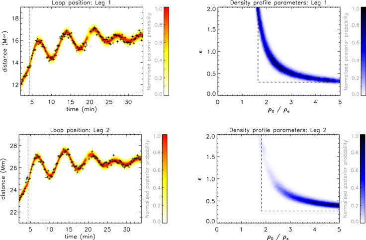
Figure 2. Seismological inversions for Leg 1 (top) and Leg 2 (bottom). The left panels show the time series for the leg positions (black crosses), while the color contour represents the normalized posterior predictive probability density for our kink oscillation model. The vertical dotted lines correspond to the maximum a posteriori probability (MAP) value for the start time of the oscillation. The right panels show normalized 2D histograms approximating the marginalized posterior probability density function for the loop transverse density profile parameters as estimated by the kink oscillation damping envelope (Equation (2)). The dashed lines outline the lower limits for the density profile parameters based on the asymptotic approximations given in Equations (14) and (15).
Download figure:
Standard image High-resolution imageIn addition to the signal-to-noise ratio, the extent to which the structuring parameters are constrained is also determined by the inverse relationships implied by τg,d (Equation (2)). The parametric curves are asymptotic in the limits  and
and  , such that is better constrained for larger density contrasts than for smaller ones. On the other hand, these asymptotes may be used to estimate lower limits for the density structure parameters.
The estimate for the lower limit of corresponds to the limit  , or
, or  . For large density contrasts, the damping profile is dominated by the exponential damping regime, so we relate it to the exponential damping rate

where the signal quality for the exponential regime is Qd = τd/Pk. This is the same approximation as Goossens et al. (2008), except for the constant of proportionality, which differs by a factor of 2/π, since we consider the linear transition layer density profile rather than the sinusoidal density profile. However, for the estimate of the lower limit of the density contrast, corresponding to  , our estimate uses the damping rate for the Gaussian damping regime (Pascoe et al. 2012, 2013, 2015; Hood et al. 2013),

where Qg = τg/Pk. These approximations are indicated by dashed lines in density profile inversion plots such as the right panels of Figure 2. They are also given in Table 2 when the temporal data alone are used, as for these cases, the upper limits are only constrained by the prior information, defined as [0, 2] for and chosen as [1, 5] for ρ0/ρe.
Figure 3 demonstrates the effect of different levels of noise in the oscillation signal on the seismological estimate of the transverse density profile parameters. For these tests, synthetic signals are generated based on the oscillation of Leg 1, with noise added to the position in the form of uniformly distributed random displacements. Results are shown for several levels of noise, the largest of which is comparable to that seen in the observational data.

Figure 3. Effect of noise on the oscillation signal (top) and the seismological estimate of the transverse density profile parameters (bottom). Results are shown for noise with a maximum absolute value of 0.05 (left), 0.1 (middle), and 0.4 Mm (right). Panels are the same as in Figure 2, with red error bars corresponding to the MAP and 95% credible intervals.
Download figure:
Standard image High-resolution image4.2. Spatial Analysis (Forward Modeling of EUV Intensity Profile)
The spatial analysis used in this paper is based on that in Pascoe et al. (2017b) but adapted for the properties particular to the loop analyzed in this paper, i.e., the contribution from both loop legs in the intensity profile rather than only one. The two intensity-enhancement structures are considered as appearing close to each other as a consequence of our particular LOS (e.g., De Moortel & Pascoe 2012) rather than physically interacting (e.g., Arregui et al. 2007b; Pascoe et al. 2007; Soler & Luna 2015). Accordingly, where the structures overlap, we calculate the total intensity as the sum of the intensity from each leg,  , along our LOS rather than summing the densities, which would produce an additional contribution ∝ρ1ρ2. Each leg is taken to have its own position (x1, x2) but the same density profile parameters (A, R, ). The contribution to the intensity profile from the external plasma is described using a linear trend for the background density. In this paper, we only apply our spatial analysis to one particular segment of the loop. Since our method assumes the loop has a circular cross-section (in this case, two circular cross-sections for the two legs), we consider a segment toward the top of the loop (where there are fewer contributions from other structures) but avoid the apex of the loop (where the intensity profile is complicated by the loop curvature).
We consider the linear transition density profile (Model L) for consistency with the seismological component of our analysis, which also assumes this profile. The results are shown in Figure 4 and demonstrate that the model is able to accurately describe the observed intensity profile and, in particular, produce a well-constrained value of . Figure 4 and the left panel of Figure 5 also show the results for the three other models that feature a finite inhomogeneous layer. The models produce similar results in terms of the density profile and forward-modeled intensity profile. We note, however, that the values of the model parameters corresponding to these similar profiles can vary significantly. In particular, each model returns different values of (see Section 6 for further discussion). The value of R defined by Model P is also significantly different from those given by the other models due to the parabolic profile being asymmetric about R inside the inhomogeneous layer. This property may also contribute to being less well constrained by Model P than by the three other models.

Figure 4. Forward modeling of the transverse intensity profile (at t = 0) using the density profiles with a finite inhomogeneous layer (Models L, N, and P). The left panels show the intensity profile (black crosses), while the color contours represent the normalized posterior predictive probability density. The vertical dotted lines show the MAP values for the positions of the two legs. The middle and right panels show histograms of the normalized layer width and loop minor radius R, respectively, based on 106 MCMC samples. The vertical dotted and dashed lines denote the MAP value and the 95% credible interval, respectively.
Download figure:
Standard image High-resolution image
Figure 5. Comparison of the transverse density profiles corresponding to the MAP values for each of the seven models considered. Legs 1 and 2 are shown in green and blue, respectively.
Download figure:
Standard image High-resolution imageWe also repeat our analysis for the other transverse density profiles described in Section 3.2, the results of which are shown in Figure 6 and the right panel of Figure 5. The results for all density profile models are also summarized in Table 1. As in Pascoe et al. (2017b), the Epstein profile produces results that are nearly identical to those of Model L, since it contains the same parameters, albeit the width of the inhomogeneous layer is expressed in terms of the steepness parameter p rather than . On the other hand, Models G and S produce different results as a consequence of having one fewer model parameter—that is, no parameter corresponding to the inhomogeneous layer—so the shape of the profile is being determined by the height (A) and width (R) alone. The results for Model G are not very different, since this loop has a wide transition layer, though the profile being too broad is evident around the outer edge of Leg 2 (x ≈ 28 Mm) in addition to the more pronounced intensity peaks near the centers of the legs. On the other hand, the absence of an inhomogeneous layer in Model S produces significant differences, particularly near the center of the intensity profile, where the intensity contributions from the two legs are superposed.

Figure 6. Comparison of different transverse density profiles for the loop. The forward-modeled transverse intensity profile is shown (as in Figure 4) for the Epstein (Model E), Gaussian (Model G), and step function (Model S) density profiles.
Download figure:
Standard image High-resolution imageTable 1. Parameters for Different Transverse Density Profile Models (Mi): Linear Transition Layer Profile (Model L), Sinusoidal Transition Layer Profile (Model N), Parabolic Transition Layer Profile (Model P), Hyperbolic Tangent Profile (Model T), Generalized Symmetric Epstein Profile (Model E), Gaussian Density Profile (Model G), and Step Function Density Profile (Model S)
| Mi | A | x1 (Mm) | x2 (Mm) | R (Mm) | |
p | KiS | KiG | KLi |
|---|---|---|---|---|---|---|---|---|---|
| L |

|

|

|

|

|
⋯ | 56.1 | 19.2 | ⋯ |
| N |

|

|

|

|

|
⋯ | 55.1 | 18.1 | 1.1 |
| P |

|

|

|

|

|
⋯ | 52.0 | 15.1 | 4.1 |
| T |

|

|

|

|

|
⋯ | 51.7 | 14.7 | 4.4 |
| E |

|

|

|

|
⋯ |

|
49.6 | 12.7 | 6.5 |
| G |

|

|

|

|
⋯ | ⋯ | 37.0 | ⋯ | 19.2 |
| S |

|

|

|

|
⋯ | ⋯ | ⋯ | −37.0 | 56.1 |
Note. Posterior summaries are given at the MAP and uncertainties by the 95% credible interval.
Download table as: ASCIITypeset image
The different density profile models can be quantitatively compared by calculating Bayes factors Bij (Jeffreys 1961; Kass & Raftery 1995):

We calculate several different Bayes factors, shown in Table 1, to compare the seven density profile models. Models S and G do not contain a finite inhomogeneous layer, so each model is compared with these using the factors KiS and KiG, respectively. The values in Table 1 support there being very strong evidence (Kij > 10) for all models over Model S (no inhomogeneous layer) and for all models except S over Model G. We find that Model L best describes the observational data, and this is quantified by the Bayes factor KLi, which is positive for all cases. We note that this Bayes factor is smallest for the comparison with Model N, reflecting the similarity of these two profiles, which the data are unable to conclusively distinguish (see further discussion in Section 6.2). The observational data therefore support our use of a transverse density profile that contains a finite inhomogeneous layer in general, and the linear transition layer profile in particular, for our analysis for this data set (beyond the practical issue that it is the only profile for which the Gaussian damping time is known). However, we may also perform our analysis using Model N if we restrict ourselves to only considering the exponential damping regime of kink oscillations (see Section 6.3).
5. Multi-model Results
In the previous section, we demonstrated that the seismological method for determining the transverse density profile of our loop based on its damped kink oscillation was not effective in constraining ρ0/ρe and , owing to the limited quality of the oscillation signal (in particular, the noise in the signal as demonstrated in Figure 3). On the other hand, the loop has a large radius, so there is sufficient spatial information for to be well constrained by forward modeling of the transverse intensity profile. These results may be used together to allow us to constrain the density contrast; i.e., if we take the estimate of ≈ 0.9 for Model L (Figure 4) and compare that with the seismological inversion (Figure 2), we can infer a density contrast of ρ0/ρe ≈ 2.3. More formally, we could repeat our seismological analysis but replace the prior information for , which we considered to have a uniform probability in the range [0, 2], with the posterior probability information from the spatial analysis (middle panel of Figure 4).
However, we are interested in developing a more general method that allows multiple physical models and data sources to be used simultaneously to constrain model parameters. To achieve this, the MCMC code used in Pascoe et al. (2017a, 2017b) has been further developed to use multiple independent variables, dependent variables, and model functions but a common set of model parameters. Each dependent variable is assigned its own measurement error σi, which is also varied as a model parameter. For a multi-model method to be an improvement over each model applied individually, the different model functions should share at least one parameter, which is the normalized inhomogeneous layer width in the case of our spatial and temporal methods.
The code makes use of the LIST data type of IDL, which is convenient for handling different observational data sets (e.g., spatial or temporal information). An approach using multidimensional arrays, for example, would require the different data sets having different numbers of data points to be taken into account.
5.1. Simultaneous Temporal Analysis of Both Legs
Our first multi-model analysis considers the time series for the two loop legs simultaneously. According to our interpretation of the oscillations as a fundamental harmonic of a standing kink oscillation, each leg has the same start time (t0), phase, and period of oscillation (determined by the initial and final values of the Alfvén transit time TA0,1). We also assume the legs have the same values of density contrast, minor radius, and inhomogeneous layer width. The model parameters that differ for each leg are therefore the amplitude of the oscillation (A1), the background trend, and the measurement error (σY).
The results of this analysis are shown in Figure 7. The top-left panel shows the oscillation of both legs and their common start time (dashed line). The density profile parameters are shown in the top-right panel. Since the analysis of each leg separately did not successfully constrain the density profile parameters, neither does this simultaneous method.

Figure 7. Seismological analysis using the oscillations of both loop legs simultaneously. Panels are the same as in Figure 2.
Download figure:
Standard image High-resolution imageWhile the loop legs appear to overlap for our LOS in EUV emission, they are physically orientated, with one being closer to us than the other. If we consider a semicircular loop, then for footpoints on the same LOS, each leg would be observed at the same height. Consequently, a standing mode would have the same amplitude in each leg. A more complicated loop geometry or inclined LOS could result in one leg having a larger amplitude oscillation than the other, but our results (Table 2) are consistent with them being equal. For the fundamental standing mode (and other odd harmonics), the legs would also have the same phase, while for even parallel harmonics, the legs would move in antiphase.
Table 2. Results of the Different Methods Presented in This Paper
| Temporal Data | Leg 1 | Leg 2 | Legs 1 and 2 | Leg 1 | Leg 2 | Legs 1 and 2 |
|---|---|---|---|---|---|---|
| Spatial Data | ⋯ | ⋯ | ⋯ | ✓ | ✓ | ✓ |
| Section | 4.1 | 4.1 | 5.1 | 5.2 | 5.2 | 5.2 |
| Bayesian Analysis | ||||||
| Oscillation start time t0 (minutes) |

|

|

|

|

|

|
| Initial Alfvén transit time TA0 (minutes) |

|

|

|

|

|

|
| Final Alfvén transit time TA1 (minutes) |

|

|

|

|

|

|
| Initial kink period Pk0 (minutes) |

|

|

|

|

|

|
| Final kink period Pk1 (minutes) |

|

|

|

|

|

|
| Gaussian damping time τg (minutes) |

|

|

|

|

|

|
| Exponential damping time τd (minutes) |

|

|

|

|

|

|
| Density contrast ratio ρ0/ρe | >1.6 | >1.8 | >1.8 |

|

|

|
| Inhomogeneous layer width |
>0.30 | >0.27 | >0.25 |

|

|

|
| Kink mode amplitude A1 (Mm) |

|

|

|

|

|

|
| Position error σy (Mm) | 0.23 | 0.21 | 0.23, 0.21 | 0.23 | 0.21 | 0.23, 0.21 |
| Intensity error σI (DN) | 1.74 | 1.74 | 1.74 | |||
| Additional Estimates | ||||||
| Kink period Pk (minutes) | 8.4 ± 0.3 | 8.4 ± 0.4 | 8.4 ± 0.3 | |||
| Kink speed Ck (Mm s−1) | 1.7 ± 0.2 | 1.7 ± 0.2 | 1.8 ± 0.2 | |||
| Internal Alfvén speed CA0 (Mm s−1) | 1.5 ± 0.2 | 1.5 ± 0.2 | 1.5 ± 0.2 | |||
| External Alfvén speed CAe (Mm s−1) | 2.2 ± 0.2 | 2.3 ± 0.3 | 2.2 ± 0.2 | |||
| Magnetic field strength B0 (G) | 11.4 ± 1.2 | 11.8 ± 1.3 | 11.6 ± 1.2 | |||
| Phase-mixing timescale τA (minutes) | 2.9 ± 1.2 | 2.6 ± 1.0 | 2.8 ± 1.1 | |||
Note. The oscillation start time t0 is measured relative to the start time of the analyzed data of 04:40 on 2011 February 10. Posterior summaries are given at the MAP and uncertainties by the 95% credible interval. Additional estimates for an estimated loop length L = 440 ± 44 Mm and a plasma density of ne = 1015 m−3 are also listed.
Download table as: ASCIITypeset image
5.2. Spatiotemporal Analysis
Since we have both loop legs present in our observational slit, we have a choice of combining the spatial information with the oscillation of Leg 1 or Leg 2. As in Section 5.1, we can also model the oscillation of both legs simultaneously and combine this with our spatial analysis, the results of which are shown in Figure 8. All three combinations produce similar results, given in Table 2. The combination of both spatial and temporal information allows the density profile parameters to be well constrained by the model.

Figure 8. Analysis based on the simultaneous use of the transverse intensity profile and the oscillations of both loop legs. Panels are the same as in Figures 2 and 4.
Download figure:
Standard image High-resolution image6. Discussion
6.1. Evolution of Transverse Density Profile
Our present method does not account for the time-dependent behavior of the transverse loop profile. Such changes may arise as a consequence of large-amplitude oscillations, e.g., the Kelvin–Helmholtz instability (KHI) or longitudinal flows driven by the ponderomotive force, or due to heating associated with the dissipation of the wave energy. In this paper, the seismological method assumes the transverse density profile does not change when calculating the kink oscillation damping profile, and our forward-modeling method is based on a single intensity profile (corresponding to before the oscillation begins).
Figure 9 shows the variation of R, , and A just before and during the oscillation. A strong negative correlation is evident in the parameters when the oscillation amplitude is greatest and with the same periodicity. The apparent quasi-periodic variation of the density profile parameters with the same period as the kink oscillation would be of interest for a follow-up study. In terms of the longer, nonoscillatory trend, the effect is much weaker, with R and each decreasing by ∼10%.
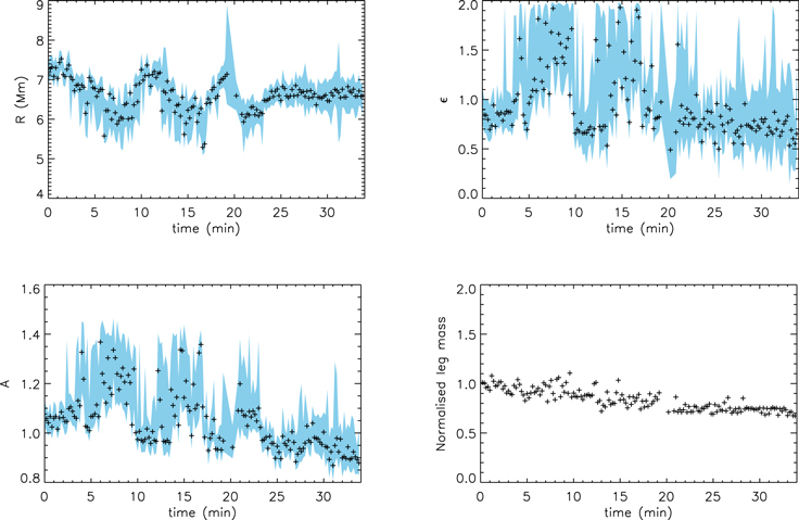
Figure 9. Time dependence of the transverse density profile parameters R (top left), (top right), and A (bottom left) as determined by forward modeling of the transverse intensity profile. The symbols indicate the MAP values, and the shaded regions correspond to the 95% credible intervals. The bottom right panel shows the corresponding variation in leg mass per unit length (normalized by its initial value).
Download figure:
Standard image High-resolution imageFigure 9 also shows the variation of the normalized leg mass (per unit length) in time based on our forward-modeled density profile. This is estimated using the MAP values of the density profile parameters (shown by the symbols in the other panels of Figure 9) to calculate the linear mass density for the observed leg segment. We note that the oscillatory behavior is not seen in this parameter but that a gradual decrease of approximately 30% is detected.
The KHI (e.g., Terradas et al. 2008a; Soler et al. 2010; Zaqarashvili et al. 2015; Magyar & Van Doorsselaere 2016; Howson et al. 2017) would cause a redistribution of mass in the perpendicular direction, whereas the ponderomotive force causes field-aligned flows toward the loop apex (e.g., Terradas & Ofman 2004). On the other hand, our slit is quite close to the loop apex, and we would also expect flows to bring material from lower down toward our slit. An alternative is that the apparent decrease is a consequence of heating (e.g., Pagano & De Moortel 2017) or cooling (e.g., Cargill et al. 2016), which causes plasma emission to become less intense in the particular 171 Å bandpass used.
6.2. Choice of Transverse Density Profile Model
In Section 4.2, we demonstrated that the values of density profile parameters such as R and vary for the different models tested; i.e., the definition of these parameters depends on the choice of profile. In particular, we may consider the linear transition layer profile (Model L) and the sinusoidal transition layer profile (Model N). Figure 10 shows the density profile described by Model N with = 2 (solid line). The density profiles for Model L with = 1.4 (dashed line) and = 2 (dotted line) are also shown. It is evident that Models L and N describe significantly different density profiles in the limit  . On the other hand, the profiles produced by L = 1.4 and N = 2 (with the density profile model denoted by the subscript) are very similar, differing mainly in the smoothness of the profile near the edges of the inhomogeneous layer. Figure 11 shows the relationship between the density profile parameters for Models L and N. For each value of 0 < N ≤ 2 considered (symbols), the density profile is generated using Model N and then compared with profiles generated by Model L to find which value of L produces the closest density profile (top left panel). We see that L < N (consistent with Figure 4) and that the limit
  corresponds to L ≈ 1.4. The bottom panels of Figure 11 show that for L ≳ 1.4, Model N has already reached the upper limit of N = 2, so the density profile can only be approximated by increasing the radius RN and decreasing the density enhancement AN. We note that the fact that Model L can describe a wider range of density profiles (by varying alone) presents an additional practical reason to favor the use of Model L in the analysis of coronal loops, or at least as an initial guess. The smoother profiles produced by Model N are likely to be more physically realistic than the piecewise profiles of Model L. However, these small differences are likely to be observationally undetectable (and, indeed, are not seen for the data analyzed in this paper), so Model L is generally more practical for the reasons discussed above.
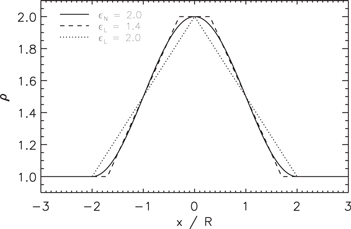
Figure 10. Comparison of density profiles produced by Model L and Model N for several values of and a density contrast ratio ρ0/ρe = 2.
Download figure:
Standard image High-resolution image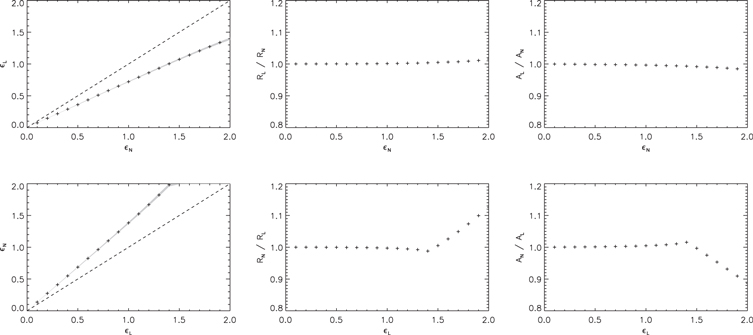
Figure 11. Relationship between density profile parameters , R, and A for Models L and N (indicated by the subscript). In the top panels, the symbols correspond to parameter values found by fitting Model L to a density profile generated by Model N. In the bottom panels, Model N is fit to a density profile generated by Model L. Shaded regions correspond to the 95% credible intervals for the model parameters.
Download figure:
Standard image High-resolution imageThe resonant absorption rate is determined by the gradient of the Alfvén speed around the resonance position (typically R). The rate is known for Models L and N for the exponential damping regime (whereas for the Gaussian damping regime, it is currently only known for Model L). We may consider a general form (e.g., Goossens et al. 2002; Roberts 2008; Soler et al. 2014),

where C = 2/π for Model N and 4/π2 for Model L. Accordingly, we see that if data cannot be used to distinguish these two profiles, then there is an uncertainty of a factor of 2/π ≈ 0.64 in the damping time τd that would affect the results of seismological information subsequently derived using this parameter. On the other hand, the density profile parameters themselves also depend on the choice of density profile shape, as we have shown. In particular, we find that our value of for Model N is approximately 1.4 times larger than that for Model L for the same observational data (see Figure 4 and Table 1). The difference in the maximum value of the density profile (which determines the density contrast ratio) is negligible, so for a more appropriate comparison of the damping rates, we can consider the factor C/ rather than C alone. For our observational data, using the MAP values for , we obtain C/ = 4/(π2 × 0.9) ≈ 0.45 for Model L and 2/(π × 1.3) ≈ 0.49 for Model N.
The systematic error expected to arise due to the unknown density profile is therefore significantly overestimated when considering the value of C alone and not including the effectively different definition of . In our case, the difference between the observed loop having a sinusoidal rather than linear density profile would contribute a factor of ≈0.92 (rather than 2/π ≈ 0.64), i.e., an uncertainty ≲10%.
The different range of density profiles produced by the different models should be taken into account when considering parametric studies. For example, Soler et al. (2014) reported that the error in the period of oscillation due to the thin boundary (TB) approximation in the limit  is ≈45% for Model L and ≈15% for Model N. This larger error for Model L is consistent with that model producing a wider range of density profiles than Model N. The error for Model L with ≈ 1.4 is comparable to that for Model N with ≈ 2 (Figure 1 of Soler et al. 2014). This smaller difference in the period of oscillation when comparing appropriate values of is also consistent with the kink mode being a collective oscillation depending on the density-weighted average of the Alfvén speed, rather than being sensitive to details of the transverse structuring (e.g., Terradas et al. 2008b; Pascoe et al. 2011).
6.3. Exponential and Gaussian Damping Profiles
In this paper, we consider both spatial (forward modeling of the EUV intensity profile) and temporal (damping rate of kink oscillation) information to constrain the transverse density profile of a coronal loop. For the seismological method, we use the GDP given by Equation (2) as the most general approximation for the damping of kink oscillations (accounting for both the Gaussian and exponential damping regimes). However, an important consideration of this study is that the particular observational data do not allow us to identify the two damping times (Figure 2), so we use the spatial information to determine independently. Given our choice of density profile (see Section 6.2), we can then determine the density contrast ratio using the observed damping time and period of oscillation. Since we are only using the seismological data to determine the damping rate (i.e., not considering the shape of the damping profile), the use of the GDP is not a necessary component of our model. For example, we can use our method of spatiotemporal analysis using only an exponential or Gaussian damping profile (with the appropriate definition of the damping time). We note that for the exponential damping profile, the method is not necessarily restricted to Model L, as it (currently) is for the Gaussian damping profile. For example, τd is also known for Model N.
Repeating our analysis as in Section 5.2 for an exponential damping profile and a Gaussian damping profile also allows us to compare the damping profile models directly using Bayes factors (Equation (16)). Comparing the version of our method using the Gaussian damping profile with the two versions using the exponential damping profile gives us KGE = 7.5 using Model L and KGE = 8.0 using Model N, corresponding to strong evidence for the Gaussian version over both exponential versions. The Bayesian evidence for the version using the GDP is, in turn, stronger than that for the versions using the Gaussian or exponential damping profiles alone; K = 3.8 (GDP over Gaussian), 11.2 (GDP over exponential with Model L), and 11.7 (GDP over exponential with Model N). We can therefore expect the inversion based on the general or Gaussian damping profile (the results of which are very similar) to be more appropriate for our observational data than that based on the exponential damping profile. The results of these additional models are shown in Table 3 (the results for the spatiotemporal method using the GDP are repeated from Table 2 for comparison).
Table 3. Comparison of Spatiotemporal Analysis Using GDP (Equation (2); see also Table 2) with Versions of the Method Using the Gaussian or Exponential Damping Profiles
| Temporal Data | Legs 1 and 2 | Legs 1 and 2 | Legs 1 and 2 | Legs 1 and 2 |
|---|---|---|---|---|
| Damping Profile | GDP | Gaussian | Exponential | Exponential |
| Density Profile | Model L | Model L | Model L | Model N |
| Section | 5.2 | 6.3 | 6.3 | 6.3 |
| Oscillation start time t0 (minutes) |

|

|

|

|
| Initial Alfvén transit time TA0 (minutes) |

|

|

|

|
| Final Alfvén transit time TA1 (minutes) |

|

|

|

|
| Density contrast ratio ρ0/ρe |

|

|

|

|
| Inhomogeneous layer width |

|

|

|

|
| Leg 1 kink mode amplitude A1 (Mm) |

|

|

|

|
| Leg 2 kink mode amplitude A1 (Mm) |

|

|

|

|
| Leg 1 position error σy (Mm) | 0.23 | 0.23 | 0.24 | 0.24 |
| Leg 2 position error σy (Mm) | 0.21 | 0.21 | 0.21 | 0.21 |
| Intensity error σI (DN) | 1.74 | 1.74 | 1.74 | 1.77 |
| Magnetic field strength B0 (G) | 11.6 ± 1.2 | 11.8 ± 1.2 | 10.2 ± 1.1 | 10.4 ± 1.1 |
| Phase-mixing timescale τA (minutes) | 2.8 ± 1.1 | 2.5 ± 1.0 | 5.9 ± 4.2 | 6.9 ± 4.4 |
Note. In the case of the exponential damping profile, we consider transverse density profile Model N in addition to Model L, which is used in all other versions.
Download table as: ASCIITypeset image
We note that the versions of the method using the exponential damping profile produce density contrast estimates that are significantly lower than those using the Gaussian or general damping profiles. On the other hand, the difference between the density contrast estimated using the exponential damping profile and Models L and N is <10%, consistent with the discussion in Section 6.2. The choice of kink oscillation damping profile therefore has a more significant effect on the seismologically inferred density profile than the choice of using Model L or Model N. The methods using the exponential damping profile also produce ≈30% higher estimates for the initial amplitude of the kink oscillation A1. The choice of damping profile can therefore influence the expected role of any amplitude-dependent behavior (e.g., Ofman et al. 1994; Goddard & Nakariakov 2016), such as nonlinear effects or instabilities. The estimate of the magnetic field strength is weakly sensitive to the density contrast ratio, so the exponential damping profile leads to an underestimate of ≈10% compared with the GDP. On the other hand, the phase-mixing timescale is more sensitive, and the exponential damping profile overestimates it by ∼100% compared with the GDP.
In addition to the Bayesian evidence supporting the Gaussian damping profile over the exponential damping profile, we can also consider the consistency of the estimates for the density contrasts with the damping profile on which they are based (e.g., the flowchart in Figure 22 of Pascoe et al. 2013). For a low-density contrast ρ0/ρe ≈ 1.5, implied by the analysis using the exponential profile, the GDP (Equation (2)) estimates that the switch from Gaussian to exponential should occur after approximately five cycles. Since our observational data only contain approximately four cycles, the exponential regime would not be appropriate for this density contrast. On the other hand, the analysis using a Gaussian damping profile suggests ρ0/ρe ≈ 2.4, for which the switch would occur after approximately 2.4 cycles, so we expect the Gaussian damping profile to apply for the majority of the observational data.
Both the Bayesian evidence for the Gaussian damping profile over the exponential one and the self-consistency of the Gaussian inversion compared with the inconsistency of the exponential inversion suggest the Gaussian damping profile is the most appropriate for these observational data. In the next section, we also compare these inversions with the results of numerical simulations.
6.4. Applicability of TB Approximation
A potential limitation on the accuracy of current seismological techniques is the use of the TB approximation. For the data analyzed in this paper, is well constrained by the intensity profile, and the value of the density contrast ratio is determined using seismological information and the analytical expressions for τg and/or τd, which are based on the TB approximation. Since is well constrained by our forward-modeling method (independent of the TB approximation), we may use our seismological estimate as a starting point to perform a parametric study for the density contrast ratio and check the accuracy of our inversion.
The effect of wide inhomogeneous layers has been investigated for the exponential damping regime by Van Doorsselaere et al. (2004; for Model N) and Soler et al. (2014; for Models L, N, and P). These studies demonstrate nonmonotonic behavior for the difference between the numerically calculated damping time and their corresponding analytical (TB approximation) values. The error in the damping time typically increases with until ∼ 0.5 before decreasing to a minimum for ∼ 1 and then increasing again for larger values of . The parametric study by Pascoe et al. (2013) considered both the Gaussian and exponential damping regimes (Model L) and demonstrated that the TB approximation remained reasonable for ≲ 0.6 for loops with low-density contrasts (ρ0/ρe ∼ 2) so long as the appropriate damping regime was considered. Ruderman & Terradas (2013) found that the analytical expression for τd underestimated the numerically calculated value and that for their largest value of = 0.3, the difference was ≈18%.
We perform 2D numerical simulations in a cylindrical geometry using a Lax–Wendroff scheme to solve the linear MHD equations as in Hood et al. (2013) and Pascoe et al. (2013). The simulations have a resolution of 2400 × 3000 in the radial (r) and longitudinal (z) directions, respectively. The numerical domain has a size r = [0, 6R], and in z, it scales with the choice of density contrast ratio to accommodate eight cycles of the kink oscillation (note that the pixel size is much smaller in the radial direction to resolve the resonant absorption in the inhomogeneous layer). The kink oscillation damping profile is determined using the radial component of velocity vr at r = 0.
Figure 12 shows the analysis of these numerical results (symbols) and the observed oscillation (color contour) using either an exponential (top panel) or Gaussian (bottom panel) damping profile (see also Section 6.3). For low-density contrasts, ρ0/ρe ∼ 2, the Gaussian damping profile provides a much better description of the damping behavior than the exponential damping profile. In terms of the GDP (Equation (2)), the switch from Gaussian to exponential occurs after approximately three cycles for ρ0/ρe = 2, which represents the majority of our observational data (approximately four cycles detected). The GDP and estimate for the switch are based on the TB approximation, while Hood et al. (2013) and Ruderman & Terradas (2013) found that the Gaussian damping profile applies for longer for larger values of .
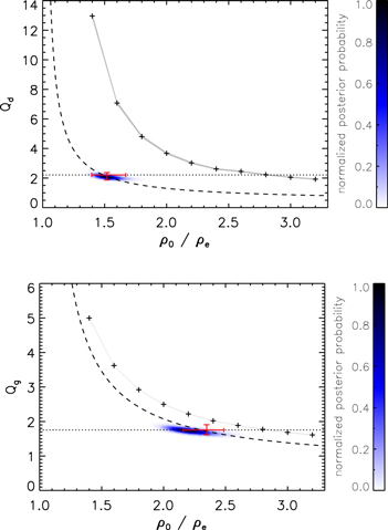
Figure 12. Analysis of numerical and observational data using an exponential (top) or Gaussian (bottom) damping profile, where the signal qualities are Qd,g = τd,g/Pk. Numerical simulations (symbols) for Model L with = 0.9 are performed for different density contrast ratios ρ0/ρe. The gray shaded regions denote the 95% credible intervals for Qd,g. The color contour represents the analysis of the observational data, with the red error bars defined by the MAP values and 95% credible intervals. The dashed curves correspond to the analytical relationships based on the TB approximation and the MAP value for .
Download figure:
Standard image High-resolution imageThe dashed curves in Figure 12 correspond to the TB approximations for the signal quality Q = τ/P. Both curves underestimate the numerically calculated values. Accordingly, we expect that these expressions will underestimate the density contrast for a given Q and . Our numerical simulations most accurately reproduce the observed damping rate for ρ0/ρe ≈ 2.8. The TB approximation using a Gaussian damping profile therefore underestimates this value by ≈18%, whereas using the exponential damping profile underestimates it by ≈46%.
The Gaussian damping profile therefore provides a significantly better estimate of the density contrast for low-density contrast loops. We note that the systematic error arising due to the use of the exponential damping profile rather than the Gaussian damping profile is greater than both the error due to the TB approximation and the possible error due to our assumption of Model L (as compared with Model N in Sections 6.2 and 6.3).
Figure 13 shows a comparison of the numerical results (colored curves) with the observational data for the oscillation of Legs 1 and 2 (circles). To allow this comparison, the observational data points have been detrended and normalized. The bottom panel shows the variation of the mean position error χ2 with density contrast ratio and has a minimum for ρ0/ρe ≈ 2.8, consistent with Figure 12. We note that for our numerical calculations with = 0.9, the thin tube approximation Ck = λ/P remains accurate to within 4%, and its dependence on the density contrast ratio implies that this difference arises due to geometrical dispersion (e.g., Figure 18 of Pascoe et al. 2013) rather than the influence of the finite inhomogeneous layer.

Figure 13. Comparison of damped kink oscillation signals (top panel) from numerical simulations (colored curves) and observational data (circles) for different values of the loop density contrast ratio ρ0/ρe. The bottom panel shows the values of χ2, which is minimum for ρ0/ρe = 2.8.
Download figure:
Standard image High-resolution image
7. Conclusions
The method of multi-model Bayesian inference we have developed for this work allows multiple data sources to be used simultaneously to constrain the model parameters. For the particular application in this paper, we considered the transverse density profile of a coronal loop that performs a flare-induced kink oscillation. Density profile parameters may be estimated independently, either by forward modeling of the transverse intensity profile or seismologically using the damping profile of the kink oscillation. For both of these methods, we use a transverse density profile with a finite transition layer, the size of which is described by the parameter . Since this same parameter is used in both models, we produced accurate constraints of the density profile parameters using both models simultaneously. This is despite each model producing poor constraints for this particular loop when applied to the same observational data individually. Specifically, the loop density contrast ρ0/ρe cannot be obtained by our forward-modeling method due to the unknown LOS depth contributing to the intensity of EUV emission in an optically thin plasma such as the solar corona. The density contrast may be estimated seismologically using the kink mode damping profile. However, for coronal loops with low-density contrast, such as the one in this paper, the seismological inversion typically produces a weak constraint on due to the asymptotic behavior (e.g., Figure 2). On the other hand, this asymptotic behavior may be used to calculate lower limits for and ρ0/ρe given by Equations (14) and (15).
Coronal loops typically have minor radii of a few Mm, so the use of the transverse intensity profile to infer the density profile is limited by the spatial resolution of modern EUV instruments. However, when used in combination with seismological estimates based on the damping of kink oscillations, the intensity profile may still provide a useful upper limit to the width of the transition layer . This is particularly useful for coronal loops with lower-density contrasts, for which the seismological inversion typically places a weak constraint on , e.g., Figure 2. Since the loop we analyze is particularly wide (R ≈ 7 Mm), it is well resolved by SDO/AIA, so the forward-modeling component of the model produces a narrow constraint on . This narrow constraint on feeds into the seismological method to narrowly constrain the density contrast ratio.
Another oscillating loop (Event 32 Loop 1 in Goddard et al. 2016) has previously also been studied using the seismological (Pascoe et al. 2017a) and forward-modeling (Pascoe et al. 2017b) methods separately. The two approaches produced consistent estimates for , corresponding to the additional assumption of an isothermal loop used in forward modeling being a reasonable one. However, owing to the high-quality time series for that oscillation, the seismological estimate of  was constrained comparably well as by forward modeling
  . The method used in this paper would therefore produce no significant improvement over previous results in that case.
The particular model used in this paper is therefore most useful for wide loops with low-density contrasts, although the general method may be applied to any observations for which multiple data sources complement each other when they can be described by a single, self-consistent physical model. The model may also be extended to include additional sources of information, such as modeling the modulation of radio emission or Doppler shifts.
Our method is based on the simultaneous use of spatial (EUV intensity profile across the oscillating loop) and temporal (kink oscillation damping profile) information. We demonstrated several variations of our method depending on the choice of models. For the kink oscillation, we considered a Gaussian or exponential damping profile (Section 6.3) in addition to the GDP, which includes both regimes (Section 5.2). For consistency, we use the same model for both the spatial and temporal components of our technique when applied simultaneously. This limits us to Model L for the general or Gaussian damping profiles, whereas for the exponential damping profile, we considered both Model L and Model N. On the other hand, we demonstrated that this choice of density model has a small effect on the inferred density profile (Section 6.2). Furthermore, for this particular observation, we found that Model L best described our observational data (Section 4.2).
Our Bayesian analysis revealed very strong evidence to prefer the results based on the general/Gaussian damping profiles over those based on the exponential damping profile (which produced a significantly lower estimate of the density contrast ratio and higher estimate of the oscillation amplitude). This was also supported by our numerical simulations, which allowed us to estimate the effect of the wide inhomogeneous layer ( ∼ 1), whereas the seismological estimates are based on the TB approximation. For the general/Gaussian damping profile, the density contrast was underestimated by ≈18%, compared with an underestimate of ≈46% using the exponential damping profile. Ensuring that the most appropriate damping profile is used is therefore the largest potential source of error in the seismological use of damped kink oscillations, compared with the effects of the TB approximation and choice of density profile model. We have not quantified the influence of nonlinear effects, though the study by Magyar & Van Doorsselaere (2016) suggests the effect of KHI is weak for ≳ 0.5. The delayed onset of KHI for loops with wider inhomogeneous layers is also evident in simulations analyzed by Goddard et al. (2018) and Pagano et al. (2018).
Future observations for which is well constrained by spatial information may be analyzed according to the procedure in this paper, i.e., using the seismological estimate as a starting point for a localized numerical parametric study to best determine the loop parameters. We note that this may be assisted by expecting as a simple initial estimate that the TB approximation typically underestimates the density contrast by ≲20% (see also Van Doorsselaere et al. 2004; Pascoe et al. 2013; Ruderman & Terradas 2013; Soler et al. 2014; Pagano et al. 2018).
An interesting component of this study is our tracking of the two overlapping legs (e.g., Figure 1). This may be considered as a first step toward future work that considers multi-threaded structures. Furthermore, we note that the methods discussed in this paper only used data from a single slit across a loop. It could be extended further to consider multiple slits, for which spatial analysis could reveal longitudinal structuring (e.g., expansion or stratification), and temporal analysis could reveal the spatial dependence of different harmonics. Additionally, the use of multiple bandpasses (forward modeled by a code such as FoMo; Van Doorsselaere et al. 2016) could allow the isothermal approximation to be relaxed and provide additional temperature and density information or multi-mode analysis to be considered (e.g., sausage modes observed in the modulation of radio emission).
This work is supported by the European Research Council under the SeismoSun Research Project No. 321141 (DJP, SAA, CRG, VMN) and the BK21 plus program through the National Research Foundation (NRF), funded by the Ministry of Education of Korea (VMN). This project has received funding from the European Research Council (ERC) under the European Union's Horizon 2020 research and innovation program (grant agreement No. 724326). The work was performed with budgetary funding of Basic Research program II.16.3.2 "Non-stationary and wave processes in the solar atmosphere" and supported by the RFBR according to the research project No 17-52-80064 BRICS-A. The data are used courtesy of the SDO/AIA team.