


Abstract
Motivated by recent analysis of solar observations that show evidence of propagating Rossby waves in coronal holes and bright points, we compute the longitudinal phase velocities of unstable MHD Rossby waves found in an MHD shallow-water model of the solar tachocline (both overshoot and radiative parts). We demonstrate that phase propagation is a typical characteristic of tachocline nonlinear oscillations that are created by unstable MHD Rossby waves, responsible for producing solar seasons. For toroidal field bands placed at latitudes between 5° and 75°, we find that phase velocities occur in a range similar to the observations, with more retrograde speeds (relative to the solar core rotation rate) for bands placed at higher latitudes, just as coronal holes have at high latitudes compared to low ones. The phase speeds of these waves are relatively insensitive to the toroidal field peak amplitude. Rossby waves for single bands at 25° are slightly prograde. However, at latitudes lower than 25° they are very retrograde, but much less so if a second band is included at a much higher latitude. This double-band configuration is suggested by evidence of an extended solar cycle, containing a high-latitude band in its early stages that does not yet produce spots, while the spot-producing low-latitude band is active. Collectively, our results indicate a strong connection between longitudinally propagating MHD Rossby waves in the tachocline and surface manifestations in the form of similarly propagating coronal holes and patterns of bright points.
Export citation and abstract BibTeX RIS
1. Introduction
Rotating stars always have the possibility of having Rossby waves, because these waves are a fundamental mode of oscillation in rotating spherical bodies. We see these waves in Earth's atmosphere and oceans, and they are surely present in the atmospheres and oceans of other planets in the universe.
Rossby waves are likely to occur when there is a domain in which the fluid or plasma has some tendency to conserve the total vorticity about a local vertical axis. Total vorticity is the sum of vorticity relative to a rotating reference frame, such as the rotating solar core, and the local vertical component of rotation, which is proportional to the sine of the latitude—so zero at the equator, maximum at the pole. Layers or shells with subadiabatic stratification are particularly favorable for Rossby waves. The solar tachocline is a good candidate.
Individual Rossby waves generally propagate in the east–west direction, retrograde relative to the reference frame if no other features, like differential rotation, are present. Rossby waves are unusual in that their group speed under the same assumptions is prograde, so a "train" of Rossby waves might be observed to be propagating prograde, even though individual waves within the train could be moving through the envelope of the train in the retrograde direction. If toroidal magnetic fields are added to the system, various forms of MHD Rossby wave modes are possible, with widely varying phase speeds, as are nearly pure Alfvén waves, if the field is strong enough. When MHD is added in the form of a toroidal field to be perturbed by waves, the resulting MHD Rossby waves can behave quite differently than their hydrodynamic (HD) counterparts, because with a magnetic field present, total vorticity (potential vorticity, which is vorticity divided by layer thickness in the case of shallow-water systems) is no longer conserved. Rotationally modified Alfvén waves are then part of the system.
A challenge in detecting Rossby waves is to distinguish between true phase propagation, whether retrograde or prograde, and intrinsic oscillations in wave amplitudes. Detecting oscillation periods alone, without information about longitude dependence, may not be enough to say definitively that a Rossby wave has been detected.
Attempts to detect Rossby waves in the Sun go back to at least the 1960s (Plaskett 1966). Sturrock (1999) claimed evidence of Rossby waves in variations of neutrino flux from the solar interior, and Kuhn et al. (2000) saw evidence for them in the shape of the solar surface, though this may instead come from aliasing from supergranulation (Williams et al. 2007). Several studies (Rieger et al. 1984; Wolff 1992; Oliver et al. 1998; Ballester et al. 2002, 2004; Dimitropoulou et al. 2008) have inferred that so-called Rieger periodicities (Rieger et al. 1984) are evidence of Rossby waves, but these periods may also, or instead, be evidence of amplitude oscillations of Rossby or other global-scale waves.
Recently, McIntosh et al. (2017) have found clear evidence of the longitudinal propagation of wavelike features seen in coronal bright points and have identified these as Rossby waves. Krista et al. (2018) have found similar evidence of propagating Rossby waves in the longitudinal evolution of coronal holes. They found retrograde phase velocities relative to the local rotation rate for latitudes 30°–55° but prograde velocities for low-latitude holes, within 10° of the equator. They also saw short-lived holes at latitudes equatorward of 65° with widely ranging phase speeds, both prograde and retrograde. Since coronal structure is largely magnetically determined, these waves almost certainly have their origin in much deeper layers, perhaps even in the tachocline. Even more recently, Löptien et al. (2018) have found evidence of HD Rossby waves in helioseismic measurements of near-surface global-scale turbulence in the convection zone. They attribute these waves to turbulent driving from smaller-scale convection.
Theoretical models of Rossby waves can take several forms, from purely linear eigenvalue models for finding frequencies of propagation (Rieger et al. 1984; Wolff 1992; Oliver et al. 1998; Schecter et al. 2001; Ballester et al. 2002, 2004; Zaqarashvili et al. 2007, 2009, 2010a, 2010b, 2015; Dimitropoulou et al. 2008; Balk 2014; Raphaldini & Raupp 2015; Gurgenashvili et al. 2017; Klimachkov & Petrosyan 2017a, 2017b; London 2017; Zaqarashvili 2018) and growth rates of unstable modes (Gilman & Fox 1997; Dikpati & Gilman 1999, 2001b, 2005; Gilman 2000; Gilman & Dikpati 2000, 2002; Cally 2003; Cally et al. 2003, 2008; Dikpati et al. 2003; Arlt et al. 2005; Gilman 2015, 2017) to fully nonlinear models that generate both phase propagation and amplitude oscillations (Dikpati 2012; Balk 2014; Raphaldini & Raupp 2015; Dikpati et al. 2018). Global models for convection, differential rotation, and magnetic fields can also show some Rossby wave propagation characteristics even for the convection zone, even though such systems generally do not produce Rossby waves per se.
Here we confine our study to the problem of longitudinal propagation of unstable Rossby modes for differential rotations thought to be typical of the solar tachocline, with dynamo-generated toroidal fields (see, e.g., Dikpati & Charbonneau 1999) of various amplitudes and of various latitudinal widths placed at various latitudes. We will use HD and MHD versions of shallow-water models applied to the tachocline (Dikpati & Gilman 2001a; Gilman & Dikpati 2002; Dikpati 2012; Dikpati et al. 2018).
Dikpati et al. (2017, 2018) showed that "seasons" of the Sun, in the form of quasi-periodic bursts of activity with periods in the range of six months to two years, can be explained as being due to tachocline nonlinear oscillations (TNOs), in which periodically varying energy exchanges occur between the preferred Rossby waves and the associated differential rotation and toroidal fields present. They simulated such TNOs using a nonlinear MHD shallow-water model with toroidal bands placed at various latitudes. This theory opens up the way to building solar season forecast models using the same system with the addition of data assimilation capability that captures surface magnetic observations and connects them to the nonlinear MHD of the tachocline. While they explained the occurrence of seasonal "bursts" as amplitude oscillations, the preferred longitudinal and latitudinal locations of the bursts, closely related to the longstanding observation of "active longitudes" (Gyenge et al. 2016, 2017), were determined largely by the phase propagation in longitude of the MHD Rossby waves excited in the system. Therefore, it is essential to capture, understand, and even predict this phase propagation. The detailed results from the study of both linear and nonlinear MHD shallow-water Rossby waves presented below provide a big step forward to predicting the location of occurrence of solar bursts.
2. Rossby Waves in "Shallow-water" Systems
The original theory of Rossby waves was based on assuming the flow in them is nearly geostrophic, that is, in near (but not exact) horizontal force balance between pressure gradients and Coriolis forces. In more modern theory, the flow is said to be at a small Rossby number Ro, which is just the dimensionless ratio between the typical rotation velocity and the rotational velocity of the interior of the spherical shell. For the solar tachocline, Ro is well estimated just from the ratio of differential rotation over a significant fraction of the distance between equator and pole to the rotation of the interior below. This ratio is of the order of 0.1, low enough to yield Rossby waves as an important component of the global HD. However, this does not mean that we have to assume a small Rossby number to solve the equations we use. In fact, it is much better to solve more general equations that contain Rossby waves as a significant, hopefully observable, part of the dynamics, but not the only part. The basics of Rossby waves in thin spherical shells, like planetary atmospheres and oceans and the solar tachocline, are discussed in Pedlosky (1987) and Regev et al. (2016).
3. Nonlinear MHD Shallow-water Model Equations
A detailed history of the development of HD shallow-water models for application in oceanic and atmospheric contexts (see, e.g., Pedlosky 1987) and their generalization to an MHD shallow-water system (Gilman 2000) for application to the solar tachocline is presented in Dikpati et al. (2018).
Although the full set of nonlinear MHD shallow-water equations has been given earlier in spherical polar coordinates in both inertial (see, e.g., Gilman & Dikpati 2002) and rotating (Dikpati et al. 2018) frames of reference, we repeat the equations here for the sake of completeness. In the rotating frame of reference (rotating with core rotation rate ωc, which is equivalent to the rotation rate at 32° at the tachocline depth), we denote h as the height change relative to the undisturbed height, u and v as the horizontal velocities in the longitude  and latitude
  directions, respectively, and a and b as the corresponding magnetic field components and write the nonlinear one-layer, dimensionless MHD shallow-water equations as

The length and time are scaled, respectively, by the radius r0 of the fluid shell and by the inverse of the interior rotation rate ( );
);  is a dimensionless parameter, in which g is the effective or reduced gravity of the stratified layer of undisturbed dimensional thickness H and
  , the fractional departure of the actual temperature gradient from the adiabatic gradient. Dikpati et al. (2017) used δ for
  , so we will use δ hereafter. The factor (4πρ)−1/2 has been absorbed into the magnetic components (ρ is the fluid density). In the overshoot part of the tachocline (located between 0.7 R⊙ and 0.72 R⊙), the value of the subadiabatic temperature gradient is
  , and in the radiative tachocline (between 0.68 R⊙ and 0.7 R⊙), its value is 10−2 ≲ δ ≲ 10−1.
Differential rotation can be expressed in the rotating frame as

in which μ is the sine latitude (sinϕ) and s0, s2, and s4 are the numerical coefficients. The interior rotation rate ωc approximately matches the rotation rate at 32° latitude at the tachocline. If s0, s2, and s4 are zero, there is no differential rotation, and all latitudes rotate at the interior rate. But for a finite differential rotation amplitude, s0 is the rotation rate at the equator, and s2 and s4 are chosen so that ω0 = 0 at 32° latitude. Then with the choice of values of s2 and s4, the differential rotation amplitude becomes (s2 + s4)/s0.
Following Dikpati & Gilman (1999), we use the same Gaussian expression to represent the spot-producing toroidal magnetic band. For the sake of completeness, we write the expression of the reference-state toroidal magnetic band ( α0 is the angular measure) as

In expression (8), f0 is the field strength, β controls the width of the Gaussian band, dsl is the sine latitude of the center of the band, and p is the prefactor to scale the peak field strength with the change in β in the Gaussian profile, so that the value of f0 denotes the peak field strength.
In addition to our nonlinear studies, we will also estimate the growth rates and phase speeds from the linear eigensystem for a shallow-water model (see the eigenvalue equations of Gilman & Dikpati 2002, which are presented in an inertial frame, but we will solve them in a rotating frame). It is important to recognize that for the global unstable modes we will find from the eigenvalue equations, both the phase velocity and the growth rate of each unstable mode are the same for all latitudes, regardless of the latitude location of the toroidal band included or the band's width in latitude.
The numerical algorithm and the technique for solving nonlinear MHD shallow-water equations for the solar tachocline, along with the initial conditions, have been discussed in detail in Dikpati (2012) and Dikpati et al. (2018). Also, the solution method for a linear eigensystem for the shallow-water solar tachocline has been discussed in Dikpati & Gilman (2001a) and Gilman & Dikpati (2002).
To formulate a double-band configuration of the toroidal field, we use a combination of two Gaussian profiles that produce two oppositely directed toroidal bands, one at a low latitude and the other at a high latitude, to mimic certain phases of an extended solar cycle (see, e.g., Cliver 2014; McIntosh et al. 2015).
The parameters chosen for both nonlinear simulations and linear calculations are differential rotation amplitude = 21% and two characteristic G values (G = 0.5 and G = 100, to characterize the overshoot and radiative tachoclines, respectively). We focus primarily on toroidal bands of 10° latitudinal width (full width at half maximum). However, we perform one set of numerical experiments using a combination of narrowband and broadband in a double-band configuration. We present our results in the following section.
4. Results
4.1. Phase Propagation of Rossby Waves during the Occurrence of TNOs
We give two examples of the longitudinal phase propagation of nonlinear MHD Rossby waves in a fully nonlinear MHD shallow-water system, which illustrate typical phase propagation behavior in solutions in which the perturbation energy amplitude itself is quasi-periodically oscillating because of energy exchanges between the waves and the differential rotation and toroidal field. These two examples are, respectively, for toroidal band placement at 40° and 30°. Both have initial peak toroidal fields of 35 kG.
4.1.1. Toroidal Field Band Peak at 40°
Dikpati et al. (2018) focused on TNOs as a possible explanation for the so-called "seasons" of solar activity. These are amplitude oscillations. But contained within them are features of phase propagation in the longitude of the dominant longitudinal wave numbers. We give examples of such phase propagation in the fully nonlinear shallow-water system. Figure 1 shows a time trace of the energy in modes m = 1–4 in a typical simulation. The simulation length is about a year in dimensional terms. We see clear evidence of nonlinear oscillation as instability begins in the m = 1 mode and spreads to higher m due to further instability and nonlinear interactions.

Figure 1. Dimensionless kinetic energy of lowest longitudinal wave numbers m as a function of time for TNO simulation. One hundred time units represents approximately one year. The effective gravity is G = 0.5, and the peak initial toroidal field is 35 kG.
Download figure:
Standard image High-resolution imageFigure 2 shows a plot of the bulges (red) and depressions (blue) of the shallow-water tachocline, and the white band represents the position of the deformed toroidal band. This time period runs about 4–8 months from beginning to end. Even though there are several longitudinal wave numbers present, one can see clearly that the whole pattern is propagating retrograde relative to the rotation of the system. If we compare this retrograde speed with those of Krista et al. (2018), with appropriate conversions between dimensionless and dimensional units and between angular and linear velocities, we can show that the retrograde speed of our example, chosen somewhat arbitrarily, falls within the range of speeds of coronal holes in the Sun.
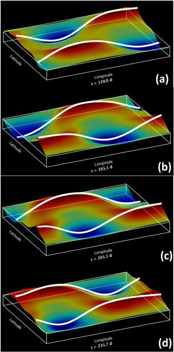
Figure 2. Longitude–latitude plots of tachocline bulges (red), depressions (blue), and deformed toroidal field (white tube). The initial toroidal field peak of 35 kG is at 40° latitude in each hemisphere. The plot is for a full circumference (360° longitude) and from pole to pole (180° latitude). Frames (a)–(d) are approximately evenly spaced in time, with time separation between 35 and 45 days. Note the relatively rapid retrograde (right to left) motion of the bulges and depressions with time.
Download figure:
Standard image High-resolution image4.1.2. Toroidal Band Peak at 30°
Figures 3 and 4 show the energy trace and longitudinal propagation of tachocline bulges, analogous to those seen in Figures 1 and 2, but for a band at 30°. In Figure 3 we see clearly the oscillations among modes with different low m after the initial transient has faded out with the growth of multiple wave numbers.
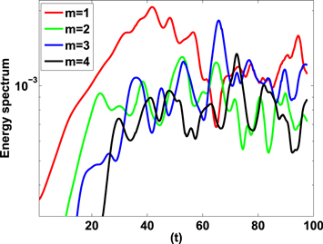
Figure 3. Same as Figure 1 but for toroidal band placement at 30° latitude.
Download figure:
Standard image High-resolution image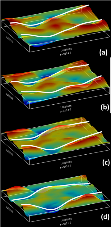
Figure 4. Same as Figure 2 but for toroidal band placement at 30° latitude.
Download figure:
Standard image High-resolution imageIn Figure 4, if we track by eye the red bulges in both hemispheres that are seen on the right edge of frame (a), we can see that there are both evolution and retrograde propagation over the next 80 days, but with total retrograde movement of no more than 40° longitude, much slower than we see in Figure 2 for band placement at 40°.
There is also some evidence of latitudinal propagation and reflection of gravity waves (the smaller-scale ripples at the right edge of frame (c), for example). The slower retrograde pattern movement is a direct result of the latitude placement of the toroidal band, which in this case is at a latitude whose local rotation is very close to that of the interior and therefore of the rotating frame itself. It is important to stress that the whole bulge, which is considerably wider in latitude than is the toroidal band, moves retrograde in a relatively coherent fashion, implying that the phase speed is more nearly global, rather than just occurring near the peak of the toroidal field.
Taken together, the results for the bands at 40° and 30° show that, as a solar cycle progresses and the toroidal bands migrate equatorward, as they must do to be consistent with the butterfly diagram for sunspots, we should expect the longitudinal phase speeds of MHD Rossby waves observable in surface magnetic and coronal data to evolve significantly, with a tendency to become less retrograde with time, perhaps even becoming prograde. This should be true even for such features that have considerably greater latitudinal extent than the toroidal field that is the source of sunspots at that phase of the cycle.
4.2. Phase Velocities of Linear Unstable MHD Rossby Waves
4.2.1. Single Toroidal Field Bands
There have been many previous analyses of unstable global MHD modes in the tachocline, as referenced in the introduction and in Dikpati et al. (2018). In all of those studies the emphasis was on finding which modes are likely to dominate in a nonlinear simulation. This was done by focusing on the disturbance growth rates mci. By contrast relatively little attention was given to the phase velocities cr of these modes, including whether they propagate prograde or retrograde relative to the reference-state interior rotation rate or even compared to the assumed tachocline latitudinal differential rotation. Here we reverse the focus, to emphasize much more the phase speed properties of unstable modes, since we would like to know how these speeds might help explain the phase speeds of coronal bright points and coronal holes (McIntosh et al. 2017; Krista et al. 2018). Growth rates are still important, because they can suggest which modes are most likely to dominate in the tachocline when many modes can be present.
For the linear case, all MHD Rossby waves separate into two classes, which we call "symmetric" and "antisymmetric" about the equator. For symmetric modes, v and a are symmetric and u, b, and h are antisymmetric about the equator; for the antisymmetric case, v and a are antisymmetric and u, b, and h are symmetric about the equator. In the nonlinear case, all variables can be split into these symmetry pairs, but in general both are present and interact. In the linear case the modes of each symmetry are linearly independent, each with its own phase velocity and growth rate.
To this end, we have calculated both phase velocities and growth rates for the fastest-growing unstable modes with specified m and equatorial symmetry, using the shooting method described in Gilman & Dikpati (2002). It is possible to find all unstable modes by using certain other methods, such as the generalized eigenvalue equation solver. However, here we focus on finding the most unstable modes, because in a numerical simulation starting from small perturbations, the fastest-growing modes usually dominate at finite amplitude. There are also, of course, many neutral modes over a wide range of m for both symmetries, and some of these may be excited by nonlinear forcing from unstable modes. We do these calculations for a sequence of toroidal bands of 10° bandwidth, placed at  , for peak toroidal fields ranging from 0 to 150 kG. Separate calculations are done for tachocline effective gravities G = 0.5, 100, characteristic of the overshoot and radiative tachoclines, respectively.
The question arises as to whether it is only magneto-Rossby waves that are unstable. What about inertia–gravity waves with energy from differential rotation and/or toroidal fields? In all the linear instability studies using a shallow-water model conducted by us and many colleagues, no unstable modes that could be characterized as inertia–gravity waves have been found, with or without magnetic fields. For example, phase velocities show no evidence of varying systematically with the effective gravity parameter G. To be unstable, modes must have phase velocities generally between the minimum and maximum rotations of the system, so they can extract energy from the differential rotation profile. Generally, gravity wave speeds, which we have obtained in the nonlinear evolution of shallow-water tachocline instabilities, are outside this range, as are inertial oscillations. Any such waves that are present propagate or oscillate too fast to develop the tilted structure needed for Reynolds stresses to extract energy from differential rotation. Therefore, gravity waves, produced during the nonlinear evolution of HD/MHD shallow-water instability simulations, have to be getting their energy from nonlinear forcing by Rossby waves, but they propagate much too fast to be playing a role in setting the phase speeds of coronal holes.
From previous results (Dikpati & Gilman 2001a, 2001b; Dikpati et al. 2003; Dikpati 2012) we know that, in general, unstable modes operate in two regimes: (a) an HD regime, present with no toroidal field, which fades out as the toroidal field is increased from zero; and (b) an MHD regime, which develops and dominates with increasing toroidal band strength but is absent when a toroidal field is absent. We shall see similar behavior here.
Figures 5 and 6 give the phase velocities (frames a, b) and growth rates (frames c, d) for the overshoot tachocline G = 0.5 case and the radiative tachocline case, respectively. Solid curves represent symmetric modes, and dashed curves represent antisymmetric modes. The phase speeds are measured relative to the rotation rate of the interior. We can see immediately that, as in previous studies, unstable HD modes have growth rates that rapidly decline to zero as toroidal field strengths reach 30 kG (see in particular the lower left of frame (c) for the m = 1 mode). Only the symmetric HD mode is unstable. The growth rates of these modes are quickly exceeded by unstable MHD modes that are not present in the HD limit, namely above just a few kilogausses. Similar results are seen for m = 2 modes (frame d). Note that the horizontal scale for m = 2 modes is expanded by almost a factor of four for figure clarity. We can also see that m = 1 modes, which represent the so-called "tipping" instability (Cally et al. 2003), dominate for peak toroidal fields above about 20 kG. In peak toroidal field ranges for which both m = 1, 2 are unstable, we see by comparing frames (2a) and (2b) that the phase velocities for both wave numbers are in the same range and have similar behavior with increasing toroidal field.
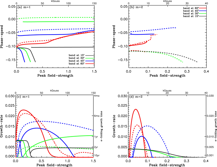
Figure 5. Phase speeds (frames a and b) and growth rates (frames c and d) for wave numbers m = 1, 2 for linear unstable MHD Rossby waves, for toroidal field band placements at 15°, 30°, 45°, and 60°, as a function of toroidal field peak strength. Solid lines denote values for symmetric modes, dashed lines for antisymmetric modes. This case is for an overshoot tachocline with effective gravity G = 0.5.
Download figure:
Standard image High-resolution image
Figure 6. Same as Figure 5 but for a radiative tachocline with G = 100.
Download figure:
Standard image High-resolution imageIn frames 5a, 5b, 6a, and 6b, we see clearly that for unstable m = 1 MHD modes, the phase velocities at  are almost independent of the field strength up to 150 kG and even beyond. At 60° for high field strengths the phase velocities increase relative to the interior rate as the toroidal field is increased, especially above about 50 kG. Antisymmetric modes, where they exist, have slightly lower retrograde phase speeds than symmetric modes. The dominant phase velocity feature is that unstable MHD modes become more and more retrograde as the latitude of the toroidal band is increased. By contrast, unstable modes of HD origin begin as strongly retrograde and become even more so as the toroidal field is increased.
There is a simple explanation for the differing degrees of retrograde phase velocity we have found for different latitude placements of the toroidal field band. We know from earlier studies (Dikpati et al. 2003) that MHD modes have peak relative amplitudes in the neighborhood of the toroidal field peak, while purely HD unstable modes (Dikpati & Gilman 2001a) have peak relative amplitudes at quite high latitudes, perhaps at 45°–55°. For all unstable modes, the phase velocity tends to be that of the local rotation rate at the latitude where the relative amplitude of the disturbance peaks. This is necessary in order to maximize the extraction of energy for perturbation growth from the reference-state differential rotation and toroidal field. When we add a toroidal band at low latitudes, instead of being an energy source, it acts as a barrier to the HD unstable mode's reaching the equator, so its peak amplitude shifts to an even higher latitude than when no fields are present, causing it to become even more retrograde. By contrast, an unstable MHD mode tends to have a phase velocity near the latitude of the peak toroidal field, so the higher the latitude of this peak, the more retrograde the disturbance. Similar arguments can be made for m = 2 modes, although they are not unstable to nearly as high peak toroidal fields.
We can quantify the relationship between the phase velocities of unstable modes and the tachocline differential rotation by plotting the angular velocities of both against latitude. For the overshoot tachocline case just discussed, Figures 7(a) and (b) show the results for G = 0.5 and G = 100 respectively. Here we have found the phase speeds in 5° intervals for unstable modes only. We see that for modes with toroidal field peaks at 30° and higher, the phase velocities are increasingly retrograde relative to the interior rate but are at the highest latitudes somewhat prograde relative to the local differential rotation rate in the tachocline. This effect is more pronounced for the overshoot (G = 0.5) than for the radiative (G = 100) tachocline. At each latitude, the length of the vertical bracket encompasses the range of peak toroidal fields, generally from zero or near zero at the bottom of the bar to 150 kG at the top of the bar. We also see that the retrograde phase velocities at a given latitude are a modest function of the peak toroidal field, illustrating the robust nature of the retrograde result.

Figure 7. Angular dimensionless phase speed ranges for linear unstable MHD Rossby waves as a function of latitude, relative to the constant rotation rate of the reference frame, which is the rotation rate of the interior. The phase speed plotted covers the range of toroidal field peaks from 0 to 150 kG. The solid curve is the differential rotation in the tachocline relative to the same reference rate. Frame (a) is for effective gravity G = 0.5, frame (b) the same for G = 100.
Download figure:
Standard image High-resolution imageFor latitudes equatorward of 30° we get quite a different result. For G = 0.5, at 25° the phase velocity is slightly prograde; for G = 100, both 25° and 20° are prograde, but then for still lower latitudes the speeds become very retrograde. No phase speed is shown for toroidal fields peaking at latitudes lower than 15°, because for these latitudes there are no unstable MHD modes. We explain above why we have found such strongly retrograde modes, which are essentially HD modes blocked from reaching the equator by the low-latitude toroidal band.
In the future, if the Rossby waves' phase speed derived from coronal hole observations, shown in Figure 4 of Krista et al. (2018), can be superimposed on our Figure 7, the combined plot could be very interesting and informative. Currently there are two issues that need to be resolved to do this: (i) Phase speeds derived from coronal hole data are valid only for four years; speed data on at least an entire solar cycle needs to be derived from coronal holes. (ii) A strategy needs to be developed for determining how the latitude of a coronal hole is related to the latitude of the underlying spot-producing toroidal field, because the correspondence between these two features is not one-to-one. Starting from the results shown in this paper, that the observational and theoretical data sets have similar longitudinal speed ranges and dependence on latitude, in a forthcoming paper we will superimpose the Rossby waves' phase speed derived from observational data on that obtained from our model.
4.2.2. Double Toroidal Field Bands
The single-band results in Section 4.2.1 naturally lead to the question of what happens if we add a second toroidal field band at high latitudes. Such a band at high latitudes in the late phases of a sunspot cycle is strongly implied by evidence for an extended cycle (Cliver 2014), for which in early phases no spots yet appear, but for which there are other signatures, such as ephemeral regions, of the existence of a subsurface toroidal band. Figures 8 and 9 show the results for two cases, for which G = 0.5 and G = 100, respectively. In both figures we present the phase velocities for unstable modes for strong ∼95 kG (frames a, b) and weak ∼10 kG bands (frames c, d) for modes with m = 1 for both symmetries. The latitudinal separation between bands is 40° in all cases. Since the phase velocities have similar profiles with latitude for very different effective gravities G, the pattern is quite robust, indicating this effect is nearly independent of where the toroidal band is in depth within the tachocline.

Figure 8. Phase velocities of unstable MHD Rossby waves when two toroidal bands of opposite signs are present in each hemisphere. The latitudinal difference in toroidal band placement is fixed at 40°. Hence the bottom and top horizontal scales for latitude are displaced by that amount from each other. The vertical scale is the toroidal band peak strength (left axis: dimensionless angular measure; right axis: dimensional values) of the high-latitude band. Frames (a) and (b) are for a strong low-latitude band of 95 kG, frames (c) and (d) for a weak band of 10 kG. Frames (a) and (c) are for antisymmetric modes, frames (b) and (d) for symmetric modes. All frames are for modes with m = 1. Darker red shading indicates more retrograde phase speed. The case shown is for an overshoot tachocline with G = 0.5.
Download figure:
Standard image High-resolution image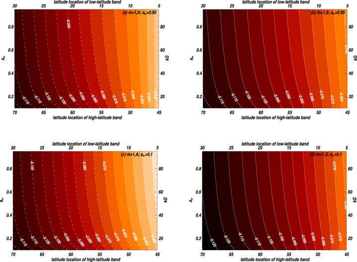
Figure 9. Same as Figure 8 but for radiative tachocline with G = 100.
Download figure:
Standard image High-resolution imageWhat we see is that, unlike a single low-latitude band, low-latitude bands are now unstable due to the presence of a high-latitude band, which prevents the formation of unstable HD modes. For most low-latitude bands, the phase velocity of the unstable mode is nearly independent of the strength of the high-latitude band, implying that the low-latitude band is the active one. This is particularly true for the case with G = 100. This is confirmed by the growth rates (not shown).
We also see that all of these modes remain retrograde for all peak fields of both bands included. However, if we were to plot the phase speeds of the double-band cases for low-latitude bands closer to the equator than 25° on Figure 7, we would find that they are much less retrograde than their single-band counterparts. Thus, there is some tendency to produce more nearly prograde propagation when a second high-latitude band is present. This is the situation likely to prevail late in a sunspot cycle, when there is a high-latitude band, but one that has not yet produced spots of the new cycle.
Are there any circumstances for which more prograde unstable MHD modes can be found? Figure 10 gives an example, for the case with G = 100. Here the low-latitude band is placed at 5° with 10° bandwidth, with a second much broader band (35° width) placed at 35°, so the separation between peaks is 30°. We see that for low-latitude bands in excess of 60 kG and high-latitude bands in excess of 40 kG, we do get sightly prograde phase speeds. If we were to add these points to Figure 7, they would be the most prograde on the plot, but still lower than the differential rotation rate in the lowest latitudes. The most likely explanation for this result is that the broad higher-latitude band confines the unstable modes to a low-latitude "channel" about the equator, and unstable HD modes are excluded from this low-latitude region. This channel actually promotes instability.

Figure 10. Similar to Figures 8 and 9 but for the case of the 10° wide low-latitude band at 5° and the 35° wide high-latitude band, with higher peak toroidal fields. Notice that here the phase velocities are now prograde.
Download figure:
Standard image High-resolution image
5. Concluding Remarks
We have shown that MHD Rossby wave phase propagation occurs in simulations of TNOs, and extensively analyzed Rossby wave phase velocities for unstable linear global MHD modes in a shallow-water model of the tachocline. We have obtained results for both overshoot and radiative tachoclines, for a wide range of toroidal band peak values and latitude placements, for both single bands and double bands with separations of 30°–40° in latitude. We find that, for single bands, the higher the latitude of band placement, the more retrograde the phase propagation relative to the rotation of the interior. Phase speed is generally relatively insensitive to the peak toroidal field strength. Single bands placed at 25° latitude produce prograde MHD Rossby waves, but those equatorward of 25° are again quite retrograde, due to the Rossby waves remaining HD and confined to latitudes poleward of the toroidal band. But when we add a second band at a higher latitude, such as may occur near the beginning of the next "extended" solar cycle, then the Rossby waves have slower retrograde speeds for the same lower-latitude band placement. If the high-latitude band is much broader in latitude than the one at low latitude, Rossby wave propagation can actually be prograde for relatively strong bands.
The model phase speeds we find overlap well with the phase speeds of coronal holes (Krista et al. 2018), becoming more retrograde with increasing latitude of band placement, among other similarities. But we must be careful to distinguish between the latitude placement of a toroidal band and the latitude of a coronal hole. In the Sun, they need not be (and probably are not) at the same latitude in general. But both can be evidence of global magnetic patterns in both the tachocline and the photosphere and corona. It is important to stress that purely HD unstable Rossby waves cannot explain the pattern of the coronal hole phase velocities that have been found, because they do not nearly have the range of phase speeds shown in Figures 7(a) and (b) for unstable MHD Rossby waves.
Future theoretical studies should focus on a much more extensive analysis of nonlinear cases, for all phases of a solar cycle. It should be possible to systematically define the relationships between TNOs and the phase propagation of Rossby waves, including simultaneous modes of several different longitudinal wave numbers. In turn, it may then be possible to make connections between these dynamical properties of the MHD tachocline and surface patterns, such as coronal holes and bright points, as well as surface magnetograms. The evolution and lifetime of both tachocline and surface Rossby wave characteristics can be compared. All of these studies, along with data assimilation procedures (see, e.g., Jouve et al. 2011; Dikpati et al. 2014, 2016; Hickmann et al. 2015) will improve our ability to simulate and predict the occurrence and evolution of active longitudes and "seasons" of the Sun (Dikpati et al. 2017, 2018).
We thank Robertus Erdelyi for reviewing the manuscript and for his helpful comments. We also thank an anonymous reviewer for his/her valuable comments on the previous version of our manuscript, which have helped significantly improve the paper. We further extend our thanks to the ISSI team of Teimuraz Zaqarashvili on "Rossby waves in astrophysics" for stimulating discussions on the topic that led to this paper. The simulation runs were performed on the Cheyenne Supercomputer of NWSC2/NCAR under project number P22104000 and the NCAR Strategic Capability project with award number NHAO0013. The National Center for Atmospheric Research is sponsored by the National Science Foundation.