


Abstract
We present a long-exposure (∼10 hr), narrowband image of the supernova (SN) remnant Cassiopeia A (Cas A) centered at 1.644 μm emission. The passband contains [Fe ii] 1.644 μm and [Si i] 1.645 μm lines, and our "deep [Fe ii]+[Si i] image" provides an unprecedented panoramic view of Cas A, showing both shocked and unshocked SN ejecta, together with shocked circumstellar medium at subarcsecond (∼0 7 or 0.012 pc) resolution. The diffuse emission from the unshocked SN ejecta has a form of clumps, filaments, and arcs, and their spatial distribution correlates well with that of the Spitzer [Si ii] infrared emission, suggesting that the emission is likely due to [Si i] not [Fe ii] as in shocked material. The structure of the optically invisible western area of Cas A is clearly seen for the first time. The area is filled with many quasi-stationary flocculi (QSFs) and fragments of the disrupted ejecta shell. We identified 309 knots in the deep [Fe ii]+[Si i] image and classified them into QSFs and fast-moving knots (FMKs). The comparison with previous optical plates indicates that the lifetime of most QSFs is ≳60 yr. The total H+He mass of QSFs is ≈0.23 M⊙, implying that the mass fraction of dense clumps in the progenitor's mass ejection immediately prior to the SN explosion is about 4%–6%. FMKs in the deep [Fe ii]+[Si i] image mostly correspond to S-rich ejecta knots in optical studies, while those outside the southeastern disrupted ejecta shell appear Fe-rich. The mass of the [Fe ii] line emitting, shocked dense Fe ejecta is ∼3 × 10⁻⁵ M⊙.
Export citation and abstract BibTeX RIS
1. Introduction
Core-collapse supernova (SN) explosions are fundamental phenomena in astrophysics. There has been considerable progress in both observational and theoretical studies of this phenomenon (e.g., Janka 2012; Müller 2017, and references therein), but our understanding of it, especially the explosion process, is still limited.
A practical approach to address the problem is to study young Galactic supernova remnants (SNRs), where we can see the footprints of SN explosions. Cassiopeia A (Cas A) is one such SNR. It is young (∼340 yr; Thorstensen et al. 2001; Fesen et al. 2006b) and nearby (3.4 kpc; Reed et al. 1995; Alarie et al. 2014). Its SN type is Type IIb, and the mass of the progenitor star has been estimated to be 15–25 M⊙ (Young et al. 2006). Our understanding of the explosion of the Cas A SN is largely based on the observational studies of shocked ejecta in optical, infrared, and X-ray bands (e.g., Fesen 2001; Hwang et al. 2004; Smith et al. 2009; DeLaney et al. 2010; Isensee et al. 2010, 2012; Fesen et al. 2011; Hwang & Laming 2012; Milisavljevic & Fesen 2013, 2015, and references therein). According to these studies, the shocked SN ejecta can be characterized into three distinct components: the 200''-diameter main ejecta ring composed of dense (∼104 cm−3) Ne- and O-burning elements, the O/S-rich "jet"–"counterjet" structure extending far beyond the main ejecta ring along the northeast–southwest direction, and the diffuse X-ray-emitting Fe-rich ejecta plumes stretching beyond the main ejecta ring in the southeast, north, and west. The estimated mass of Fe-rich ejecta is ≲0.1 M⊙, which is comparable to the expected Fe ejecta mass from complete Si burning (Hwang & Laming 2012). Models for 3D spatial distribution of these ejecta materials and their spatial relations have been developed (DeLaney et al. 2010; Milisavljevic & Fesen 2013).
In addition to the shocked ejecta, unshocked SN ejecta in the interior preserving the pristine information at the time of explosion have been detected. Alpha elements, e.g., O, Ne, Si, S, and Ar, have been detected in faint mid-infrared (MIR) emission by Spitzer Space Telescope and also in the [S iii] λλ9069, 9531 lines (Smith et al. 2009; DeLaney et al. 2010; Isensee et al. 2010; Milisavljevic & Fesen 2015), while 44Ti tracing 56Ni (and therefore its stable daughter nucleus 56Fe) has been detected in hard X-rays (Grefenstette et al. 2014). The unshocked S ejecta have a sheet- or bubble-like morphology, suggesting bubbles of radioactive 56Ni-rich ejecta. On the other hand, the distribution of 44Ti is elongated along the east–west direction, indicating an asymmetric SN explosion. Three-dimensional numerical simulations demonstrating that neutrino-driven explosions can explain the shocked diffuse Fe plumes as well as the asymmetric 44Ti distribution have been published (Orlando et al. 2016; Wongwathanarat et al. 2017).
The morphology and nature of the unshocked SN ejecta in Cas A, however, are still uncertain. First, Fe associated with 44Ti has not been detected. This could be because the associated Fe is diffuse and cool (∼40 K; DeLaney et al. 2014; Lee et al. 2015), but that needs to be confirmed. Second, the Spitzer MIR images of O, Si, and S emission lines suggest that the unshocked SN ejecta have complex structures that might be directly related to the SN explosion dynamics, but their coarse spatial resolution (6''–10'') prevents a detailed view of the morphology. Low-frequency free–free absorption measurements yielded a mass as large as ∼3 M⊙ in the unshocked ejecta (Arias et al. 2018; see also DeLaney et al. 2014). Finally, there is another form of shocked dense (∼104 cm−3) Fe recently detected in the main ejecta ring with near-infrared (NIR) spectroscopy (Lee et al. 2017). Those spectra show essentially only Fe lines, in contrast to the spectra of Ne- and O-burning ejecta dominated by S lines, suggesting the presence of unshocked Fe ejecta in the interior. Lee et al. (2017) further pointed out that the SW shell is prominent in NIR [Fe ii] emission (see also Rho et al. 2003) and proposed that those regions are likely to be dominated by shocked dense Fe ejecta based on comparison between the distribution of the NIR Fe line emission and those of the 44Ti and X-ray Fe line emission.
Cas A also provides a unique opportunity to study the mass-loss history of the progenitor system immediately prior to the explosion. From the early optical studies of the source, it was realized that the knots in Cas A are composed of two distinct components with very different kinematic and chemical properties, i.e., "fast-moving knots" (FMKs) and "quasi-stationary flocculi" (QSFs; Minkowski 1959; van den Bergh & Dodd 1970; Peimbert & van den Bergh 1971; van den Bergh 1971; Kamper & van den Bergh 1976). Fast-moving (≳5000 km s−1) FMKs are O/S-rich SN ejecta material, while QSFs, which are almost "stationary" (≲500 km s−1) and bright in Hα and [N ii] λλ6548, 6583 emission line images (van den Bergh 1971; van den Bergh & Kamper 1985; Lawrence et al. 1995; Fesen et al. 2001; Alarie et al. 2014), are probably dense CNO-processed circumstellar medium (CSM) that has been swept up by the SN blast wave. There are about 40 QSFs scattered both inside and outside the main ejecta shell, and, from the proper-motion studies of QSFs, an expansion timescale of ∼11,000 yr was derived (van den Bergh & Kamper 1985). QSFs, however, have been studied mainly in the optical band, where the extinction is very large, i.e., AV ≳ 6 mag (see, e.g., Koo & Park 2017, and references therein), so that it is quite possible that many other QSFs remain undetected.
In this paper, we present a long-exposure (∼10 hr) image of Cas A obtained by using a narrowband filter centered at the 1.644 μm line with the United Kingdom Infrared Telescope (UKIRT) 3.8 m telescope (hereafter "deep-[Fe ii]+[Si i] image"). In the band, there are two strong lines: [Fe ii] at 1.64355271 μm  ) and [Si i] at 1.6454533 μm
  .5
The [Fe ii] 1.644 μm line is one of the strongest NIR emission lines in shocked dense atomic gas (e.g., Koo et al. 2016), tracing both shocked SN ejecta material and shocked CSM. The [Si i] 1.645 μm line could be "bright" in unshocked SN ejecta as we will see in this paper. The organization of the paper is as follows. In Section 2, we describe our observations and image processing. In Section 3, we first briefly discuss the two emission lines in the band. Then we present our deep [Fe ii]+[Si i] image and discuss new features that have not been seen either in previous low-sensitivity images (e.g., Rho et al. 2003) or in other wave-band images. In Section 4, we identify QSFs and FMKs in the deep [Fe ii]+[Si i] image and present their catalog. In Sections 5 and 6, we investigate the physical properties of QSFs and FMKs, respectively, and discuss the implications. Finally, in Section 7, we conclude and summarize our paper.
.5
The [Fe ii] 1.644 μm line is one of the strongest NIR emission lines in shocked dense atomic gas (e.g., Koo et al. 2016), tracing both shocked SN ejecta material and shocked CSM. The [Si i] 1.645 μm line could be "bright" in unshocked SN ejecta as we will see in this paper. The organization of the paper is as follows. In Section 2, we describe our observations and image processing. In Section 3, we first briefly discuss the two emission lines in the band. Then we present our deep [Fe ii]+[Si i] image and discuss new features that have not been seen either in previous low-sensitivity images (e.g., Rho et al. 2003) or in other wave-band images. In Section 4, we identify QSFs and FMKs in the deep [Fe ii]+[Si i] image and present their catalog. In Sections 5 and 6, we investigate the physical properties of QSFs and FMKs, respectively, and discuss the implications. Finally, in Section 7, we conclude and summarize our paper.
2. Observation and Image Processing
The narrowband [Fe ii]+[Si i] filter images and H-band images that we present in this paper were taken with the Wide-Field Camera (WFCAM) on the UKIRT 3.8 m telescope in 2013 September. WFCAM is equipped with four Rockwell Hawaii-II HgCdTe infrared focal plane arrays. Each array has 2048 × 2048 pixels, providing a 13 65 × 1365 field of view (FOV) with a pixel scale of 04 pixel–1. The arrays are arranged in a square pattern with a gap of 1283 between them. Since the FOV provided by a single array is significantly larger than the entire Cas A, we took images of Cas A flipping between two arrays on the east (arrays 2 and 3) so that the exposure while the Cas A is placed on the other array can be used for flat-fielding and sky subtraction. For each pointing, images were obtained at five jitter positions offset by (±64, ±64) in R.A. and decl. We performed a 2 × 2 microstep about each jitter position, with an offset size of 139, in order to fully sample the point-spread function (PSF). Five jitter positions with 2 × 2 micro-stepping give a total of 20 images. In summary, a single set of exposures provides two sky-subtracted images (one for array 2 and the other for array 3), with a total per-pixel integration time of 20t s, where t is the exposure time of each image. For the [Fe ii] and H filters, t = 20 and 5 s, respectively. In the period of 2013 September 4–13, a total of 44 sets are obtained for [Fe ii] and 14 sets for H. In our observations, we used the same [Fe ii] filters developed for the UWIFE survey (Lee et al. 2014a). They have a central wavelength of 1.642–1.645 μm with a peak transmittance of ∼85% and effective bandwidth of 0.028 μm.
Combining all the images obtained with the two arrays results in an [Fe ii]+[Si i] image with an effective net exposure time of 10 hr and an H image with 0.8 hr. This "deep [Fe ii]+[Si i] image" has a pixel size of 02, and its median PSF is 07. An astrometric calibration is done by comparing the positions of more than 100 bright, isolated stars in the field with the Two Micron All Sky Survey (2MASS) H-band catalog (Skrutskie et al. 2006). The 1σ uncertainty in astrometry is 0104 (or 0.52 pixels). For the photometric calibration, we used H-band magnitudes of 2MASS catalog stars assuming the zero-magnitude flux of 3.27 × 10⁻⁸ erg cm−2 s−1 for the [Fe ii] narrowband filter (Y.-H. Lee et al. 2018, in preparation). The flux calibration uncertainty (1σ) is 4%. The continuum-subtracted image presented in this paper is produced following the procedure in Lee et al. (2014a). The sensitivity (1σ) of the continuum-subtracted deep-[Fe ii]+[Si i] image is about 2.6 × 10⁻¹⁸ erg cm−2 s−1 pixel−1. The flux of [Fe ii] emission features derived from the continuum-subtracted image will be underestimated because there are several bright [Fe ii] lines in H band (1.5–1.8 μm; see Table 1 of Koo et al. 2016). The scaling factor depends on electron density (ne) and temperature (Te) of the source, e.g., 1.16–1.32 for gas at ne = 103–105 cm−3 and Te = 7000 K, and we will be using 1.2 in this paper.
A caveat for our image is that the [Fe ii]+[Si i] filter has a width of ±2600 km s−1, so the high-velocity ejecta could have been missed in our image. For example, the bright ejecta filaments in the northern interior have high positive and negative velocities (Milisavljevic & Fesen 2013), and they appear as negative features in our [Fe ii]+[Si i] image because we subtracted the H-band image. But such instrumental "artifacts" are limited to the northern central region, and we are seeing most of the ejecta material.
3. Deep [Fe ii]+[Si i] Image and New Features
3.1. Prelude: Is the Emission [Fe ii] or [Si i]?
Before we look at the deep [Fe ii]+[Si i] image, it would be helpful to have some discussion about the two emission lines in the band. Nebular emission at 1.64 μm is generally assumed to be the [Fe ii] 1.644 μm line. NIR spectra of a wide variety of shock waves in HH objects and SNRs confirm this by showing a wealth of other [Fe ii] lines, the strongest being the one at 1.257 μm (e.g., Gerardy & Fesen 2001; Koo et al. 2013; Lee et al. 2017). However, NIR spectra of SN 1987A (Kjær et al. 2010) and the nebular phase of the SN iTPF15eqv (Milisavljevic et al. 2017) show that the line is mainly the [Si i] 1.645 μm line, because the other [Fe ii] lines are weak or absent and also because the [Si i]  companion line at 1.607 μm is present. The [Si i] 1.607 μm line originates from the same upper level as the [Si i] 1.645 μm line, so that its intensity ratio to the [Si i] 1.645 μm line is given by the ratio of their Einstein A-coefficient, which is (7.14 × 10⁻⁴)/(2.01 × 10−3) ≈ 1/3.
For Cas A, NIR spectra of the main ejecta shell and several FMKs and QSFs have been obtained (Gerardy & Fesen 2001; Koo et al. 2013; Lee et al. 2017). Their spectra show many other [Fe ii] lines, including the strongest 1.257 μm line but no [Si i] 1.607 μm line except for a few FMKs at a level of ≲10% of the [Fe ii] 1.644 μm line intensity (see Table 3 of Lee et al. 2017). The nondetection of [Si i] 1.607 μm in most regions suggests that the emission from the shocked material in the deep [Fe ii]+[Si i] image is dominated by [Fe ii] emission. In the Appendix, we present the results of shock model calculations for the [Si i] line brightness in radiative atomic shocks. Note that the [Si i] line is not included in most of the shock models in the literature, and there is little recent atomic data for the line. We have scaled the [C i] λ9850 line flux to estimate the [Si i] brightness, which is similar to the Si i line in the behavior of its excitation rate with temperature and in the ionization fraction of C i. We have run shock models with QSF parameters and found flux ratio F[Si i]1.645/F[Fe ii]1.644 ≲ 2% in these models. Therefore, for QSFs, the 1.64 μm emission should be dominated by the [Fe ii] line. We have also run shock models for FMKs and found F[Si i]1.645/F[Fe ii]1.644 ≲ 10% when the abundances of Si and Fe are comparable (see Figure 13). The abundances of Si and Fe in FMKs are not observationally constrained and might vary substantially. Indeed, among the 56 ejecta knots identified along the main ejecta shell by Lee et al. (2017), only three of them show the [Si i] 1.607 μm line. The inferred F[Si i]1.645/F[Fe ii]1.644 ratio is 0.9 in one of them, while it is ≲0.3 (3σ) in the other two. Therefore, the Si abundance of FMKs does not seem to be significantly greater than their Fe abundance, and the 1.64 μm emission from the dense shocked ejecta material in the deep [Fe ii]+[Si i] image is probably dominated by [Fe ii] emission too.

Figure 1. Top: our deep [Fe ii]+[Si i] image of Cas A obtained from the UKIRT 3.8 m telescope. Stellar sources have been removed. The gray scale varies linearly from −2 × 10⁻¹⁸ to 2 × 10⁻¹⁷ in erg cm−2 s−1 pixel−1. Bottom: same as the top panel, but with QSFs and FMKs marked by magenta and cyan contours, respectively (see Section 4). The red star represents the explosion center at (α, δ)J2000 = (23h23m27 77, +58°48'494) determined from the proper motion of FMKs (Thorstensen et al. 2001), while the yellow contour marks the outer boundary of the SNR in radio corresponding to the intensity level of 0.3 mJy beam−1 in a VLA 6 cm image (DeLaney 2004).
Download figure:
Standard image High-resolution imageThe diffuse emission from the unshocked ejecta is a different case. The ejecta are cold and neutral shortly after the explosion, but they are subsequently ionized and heated by EUV and X-ray photons from the SNR. Models of the time-dependent ionization and heating of the ejecta show that the gas can reach temperatures of 104 K or higher (Blair et al. 1989; Sutherland & Dopita 1995; Eriksen 2009), though dust was not included in the models, and that could significantly reduce the temperature. Observations, however, suggest a much lower temperature, e.g., Te ≲ 100 K (Arias et al. 2018). As we discuss in Section 3.3, we have no theoretical reason to prefer either the [Si i] or [Fe ii] identification for the 1.64 μm line in the diffuse ejecta. But because the diffuse emission is closely correlated with Spitzer [Si ii] emission and because there is little [Fe ii] Spitzer emission in that region (Isensee et al. 2010), we will assume that the diffuse emission is [Si i]. We will discuss the emission of unshocked ejecta in more detail in Section 3.3.
3.2. Overall Morphology
Figure 1 shows our deep [Fe ii]+[Si i] image of the Cas A SNR. The overall morphology of the remnant is not very different from what has been seen in previous optical or MIR images, but, with subarcsecond angular resolution and continuum subtraction, it gives an unprecedentedly clear and panoramic view of the remnant. In particular, it shows in detail the complex structure of the faint diffuse emission in the interior that might be from the unshocked SN ejecta (see also Figure 2). We can see interesting structures, e.g., a semicircular arc structure surrounding the explosion center and protrusions from the southwestern ejecta shell pointing toward the explosion center, which presumably had been produced during the explosion. Figure 1 also reveals the disrupted western part of the main ejecta shell that has not been seen in optical observations owing to large extinction. We can see faint clumps that might be the fragments of a disrupted shell, as well as bright and faint knots scattered in this area. These new features will be discussed in the following sections (Sections 3.3 and 3.4).

Figure 2. Left: interior diffuse emission of Cas A in the deep [Fe ii]+[Si i] image. Some prominent features are labeled. The red star represents the explosion center. The contours are at levels 1 × 10⁻¹⁸ and 2 × 10⁻¹⁸ erg cm−2 s−1 pixel−1. Top right: Spitzer [O iv]+[Fe ii] 25.9 μm image of Cas A. Bottom right: Spitzer [Si ii] 34.81 μm image of Cas A. The [Si ii] line is broad (−4000 to +3500 km s−1), with blue- and redshifted velocity peaks at −2000 and +2500 km s−1, respectively (Isensee et al. 2010). The above Spitzer images are obtained by integrating over the limited velocity ranges to match the velocity range of the deep [Fe ii]+[Si i] image.
Download figure:
Standard image High-resolution imageThe most prominent emission feature in Figure 1 is the bright main ejecta shell of 200'' diameter. Its brightness distribution is very similar to those of O, Ne, S, and Ar ejecta seen in optical and Spitzer MIR images (Hammell & Fesen 2008; Smith et al. 2009; DeLaney et al. 2010; Fesen & Milisavljevic 2016), so that most of the emission in the main ejecta shell is probably from dense SN ejecta swept up by the reverse shock. And the emission that we see in the deep [Fe ii]+[Si i] image is probably predominantly [Fe ii] emission. According to 1D SN models (e.g., Woosley & Weaver 1995), Fe in the main ejecta shell might be composed of 56Fe atoms of interstellar origin, i.e., 56Fe atoms dumped into the progenitor star during its formation, and 58Fe atoms synthesized by the s-process during He core and He shell burning. In the O-rich core of a 15 M⊙ progenitor, the abundances of these two isotopes are comparable and X(O)/X(Fe) ∼ 103 in mass (Rauscher et al. 2002; see also Figure 5 of Koo et al. 2013). But 3D simulations suggest that it could be mainly Fe newly synthesized in explosive burning and mixed with O-rich ejecta owing to hydrodynamic chemical mixing (see, e.g., Figure 3 of Hammer et al. 2010; Koo et al. 2013). The bright southern shell, for example, appears to be dominated by Fe-rich ejecta (Rho et al. 2003; Lee et al. 2017).
Other prominent features in Figure 1 are numerous compact knots scattered over the remnant. They are QSFs and FMKs. The [Si i] 1.645 μm emission might be negligible compared to [Fe ii] 1.644 μm emission for these shocked clumps too, perhaps except some FMKs. The clumps surrounded by magenta contours in Figure 1 are QSFs (see Section 4). We can see that the bright clumps are mostly QSFs. The most prominent QSF feature is the large arc structure in the southwest that was previously detected in Hα and [N ii] observations (Lawrence et al. 1995; Fesen et al. 2001; Alarie et al. 2014). On the other hand, the clustered QSFs in the western area are newly discovered. We discuss the spatial distribution and physical properties of QSFs in Section 5.
In Figure 1, essentially all knots surrounded by cyan contours are FMKs outside the main ejecta shell, and our continuum-subtracted image provides a clear view of their overall distribution. The most prominent FMK features are the "jet" and "counterjet" structures in the northeastern and southwestern areas, respectively. These jet structures are enriched with S, and they have been studied in detail by using optical and NIR forbidden S lines (Fesen et al. 2006a; Hammell & Fesen 2008; Milisavljevic & Fesen 2013; Fesen & Milisavljevic 2016). They are almost undecelerated and thought to have been ejected from the innermost region at the time of core collapse by an explosive, jet-like mechanism (Fesen & Milisavljevic 2016). However, no Fe-rich ejecta knots expected in the jet-induced explosion models have been reported in the jet area (Fesen & Milisavljevic 2016). Our image shows that some FMKs outside the disrupted eastern shell appear very bright in [Fe ii] emission, while they are relatively faint in the Hubble Space Telescope (HST) F098M image obtained by WFC3/IR (Fesen & Milisavljevic 2016; hereafter the "HST F098M" image). The HST F098M image is dominated by ionized S lines, i.e., [S iii] λλ9069, 9531 and [S ii] λλ10287–10370, so that their difference in appearance suggests that these knots could be Fe-rich. It is worthwhile to note that this is where an Fe-rich diffuse X-ray ejecta plume is present (Hwang et al. 2004; Hwang & Laming 2012). In Section 6.1, we will compare the [Fe ii] fluxes of FMKs to their HST F098M fluxes.
3.3. Diffuse Emission in the Interior
Our deep [Fe ii]+[Si i] image reveals for the first time the detailed structure of the faint diffuse emission in the interior, well inside the reverse shock (Figure 2). The emission features have the form of clumps, filaments, and arcs, most of which are distributed in the central eastern and southern areas. Some prominent features are (1) interior diffuse clumps (IDC 1 to IDC 4), (2) the semicircular "Eastern Arc" of radius 30'' surrounding IDC 1, (3) "pillars" protruding from the southwestern main ejecta shell, and (4) the diffuse emission permeating through the southern main ejecta shell. The spatial location and morphology suggest that the interior diffuse emission is probably from the unshocked SN ejecta, and the above features should be closely related to the explosion dynamics. For example, the location and morphology of the Eastern Arc match the bubble-like structure seen in [S iii] lines (Milisavljevic & Fesen 2015) and could be a footprint of an Ni bubble. The pillars are also interesting. There are at least two pillars, each of which is 30''–45'' (or 0.49–0.74 pc) long, and they are pointing almost exactly to the explosion center. The morphology of these pillars is similar to the Rayleigh–Taylor fingers developing during the explosion at the Si/O interface, although they appear to point inward not outward as shown in numerical simulations (Kifonidis et al. 2003).
If the 1.64 μm emission is [Fe ii] 1.644 μm emission from Fe synthesized in SN explosion, we may expect to see some correlation with the 44Ti emission, because they are both products of α-rich Si burning. The distribution of 1.64 μm emission, however, shows no correlation with the 44Ti emission that is distributed along the east–west direction (Grefenstette et al. 2014). Instead, the overall spatial distribution of the 1.64 μm emission matches well with that of the faint [Si ii] 34.81 μm emission seen in Spitzer observations (Figure 2), which was proposed to be from unshocked SN ejecta heated by UV/X-ray emission from the reverse shock (Isensee et al. 2010). Furthermore, [Fe ii] 17.94 and 25.99 μm lines were not detected in the interior in Spitzer observations (Smith et al. 2009; DeLaney et al. 2010; Isensee et al. 2010; see also Figure 2). There is strong [O iv] + [Fe ii] 25.9 μm emission, but Isensee et al. (2010) showed that its line profile matches well with the other line profiles when we assume that the emission is entirely from O iv. These MIR characteristics suggest that the interior diffuse emission is mostly, if not all, [Si i] 1.645 μm emission, not [Fe ii] 1.644 μm emission.
On the other hand, Si atoms (I.P. = 8.15 eV) in the unshocked SN ejecta are expected to be ionized by UV photons from the reverse shock, which will be dominated by the O vi λλ1032, 1037 doublet (Hamilton & Fesen 1988). These UV photons may be attenuated by SN dust in the Cas A interior, so the inner part of the ejecta can be shielded. NIR to submillimeter observations indicate that there is a large amount (≥0.1–0.2 M⊙) of newly formed dust mixed with unshocked SN ejecta in the interior (Dunne et al. 2009; Barlow et al. 2010; Sibthorpe et al. 2010; Arendt et al. 2014; De Looze et al. 2017). Si atoms can also be ionized by X-ray photons, but if there are not enough photons, some fraction could be in a neutral form. According to low-frequency radio observations, the characteristic temperature of the unshocked SN ejecta is ≲100 K (Arias et al. 2018), in which case the collisional excitation of the [Si i] 1.645 μm line is very inefficient because of the Bolzmann factor  , and the emission from recombination would probably dominate. Since neither the abundances nor the ionization states of elements in the diffuse emission region are known, we have no theoretical reason to prefer either the [Si i] or [Fe ii] identification for the 1.64 μm line in the diffuse ejecta. However, based on the fact that diffuse emission is strongly correlated with the Spitzer [Si ii] emission and that there is little Spitzer [Fe ii] emission in that region (Isensee et al. 2010), we tentatively conclude that the diffuse emission is [Si i].6
3.4. Western Area
Figure 3 gives an enlarged view of the western area, showing the complex and clumpy structure of this region. Over a 1'-long arc, the bright main ejecta shell is missing but filled with clumps of different brightness that are ≲20'' in size, some of which are well beyond the main ejecta shell. The brightest clumps have relatively sharp outer boundaries, while the faint clumps appear fuzzy. Some bright clumps appear embedded in an extended faint envelope. In Figure 3, we show another [Fe ii] image of Cas A obtained in 2008 (Lee et al. 2017; see Section 4.2) for comparison. The 2008 image has a lower sensitivity, so that faint clumps in the deep [Fe ii]+[Si i] image are not visible. For the clumps seen in both the 2008 and 2013 images, we measure their proper motions and explore their nature, i.e., FMK versus QSF, in Section 4, but from Figure 3 it is clear that the bright clumps (marked by magenta contours) do not show measurable proper motions, indicating that they are QSFs. The nature of these clumps can be confirmed by comparing to the HST F098M image, which is also shown in Figure 3. For example, the large clump marked as Clump A is bright in the HST image but faint in [Fe ii], as are the small clumps marked as Clump B. These clumps are located in the missing portion of the main ejecta shell, so that they are likely the fragments of the disrupted ejecta shell. The overall morphology is indeed similar to that of the fragmented shell disrupted by dense ejecta knots launched just outside the Fe core in numerical models (see, e.g., Figure 10 of Orlando et al. 2016). On the other hand, the bright clumps marked by magenta contours are only barely visible in the HST F098M image, supporting their QSF nature because QSFs are faint in [S ii] and [S iii] lines. Some large QSFs appear to be embedded in a diffuse faint envelope of ejecta material, which seems to indicate their physical interaction. In Section 5.2, we discuss the lifetime of QSFs and show that most QSFs are likely to survive until they encounter the ejecta shell, where they experience a strong shock and are destroyed. These QSFs, if they are indeed interacting with ejecta material, must have been relatively recently swept up by the reverse shock.

Figure 3. Enlarged view of the western area of Cas A: [Fe ii]+[Si i] image obtained in 2008 August (Lee et al. 2017), deep [Fe ii]+[Si i] image obtained in 2013 September, HST F098M image obtained in 2011 November (Fesen & Milisavljevic 2016), and VLA 6 cm image (DeLaney 2004). The magenta contours mark the boundary of QSFs identified in the deep [Fe ii]+[Si i] image (see Section 4), while the blue contours represent the areas brighter than 4 × 10⁻¹⁸ erg cm−2 s−1 pixel−1 in the same image.
Download figure:
Standard image High-resolution imageThe western area is where radio synchrotron emission shows distinct characteristics. In this region, the radio brightness is enhanced, as we can see in the VLA image in Figure 3. The spectral index is steep, and the motions of radio-bright knots are significantly nonrandom, with some knots moving inward, indicating interactions of SNR blast wave with dense medium (Anderson et al. 1995; Anderson & Rudnick 1996; Keohane et al. 1996). The electron density in this region derived from X-ray analysis, however, is not particularly large (Hwang & Laming 2012). There is a molecular cloud at vLSR = −40 km s−1 superposed to this area, and it has been proposed that this molecular cloud is responsible for such distinct characteristics (Keohane et al. 1996; Kilpatrick et al. 2014, 2016). Most of the molecular gas, however, lies in the foreground of Cas A (see Krause et al. 2004; Wilson & Batrla 2005; Dunne et al. 2009). Also, we do not see [Fe ii] emission due to the blast wave–molecular cloud interaction as we often see in other SNRs interacting with molecular clouds. (Nor do we see H2 2.122 μm emission in our 600 s integration H2 narrowband image obtained by using the Wide-field Infrared Camera attached to the Palomar 5 m telescope.) The large population of QSFs in our deep [Fe ii]+[Si i] image instead suggests a denser CSM there. Hence, another possible explanation for the anomalous radio properties in the western area seems to be the interaction with dense clumpy CSM and the shell fragments. It is well established that, if the medium is clumpy, the flow behind a strong shock becomes turbulent and magnetic field can be amplified (e.g., Inoue et al. 2009), so we expect to see enhanced radio synchrotron emission.
4. Identification and Classification of Knots in the Deep [Fe ii]+[Si i] Image
4.1. Identification of Knots
We identified knot features in the deep [Fe ii]+[Si i] image in an automated manner. We first smoothed the continuum-subtracted, deep [Fe ii]+[Si i] image using the SMOOTH function in IDL, which makes a smoothed image with a boxcar average of the specific width, three pixels in this case, and estimated the background of the image to determine a threshold for the identification of knots. The background value and standard deviation (σ) estimated from several source-free regions of the image are (−0.35 ± 8.0) × 10−19 erg cm−2 s−1 pixel−1. We detected the knot features outside (i.e., not superposed on) the main ejecta shell using the threshold of 4 × 10⁻¹⁸ erg cm−2 s−1 pixel−1 (or 5σ above the background), a threshold that is low enough to include faint emission but high enough to exclude background noise. We have drawn the contours on the image by the threshold and defined them as "knots" after excluding residual features left from continuum subtraction, artificial patterns from the detectors, and the small contours with less than five pixels considering the pixel scale (02) and seeing (≲1''). The total number of knots detected and cataloged outside the main ejecta shell is 258.
We fitted each contour by an ellipse using the IDL procedure FIT_ELLIPSE from Coyote IDL Library7 to derive their geometrical parameters, i.e., the central coordinates, major and minor axes, and position angles (P.A.; from north to east), while the area and [Fe ii] flux were directly estimated from the contours. The uncertainty in flux estimation is ∼10%. The derived parameters are listed in Table 1.
Table 1. Catalog of Knots in the Deep [Fe ii] + [Si i] Image
| ID | α(J2000) | δ(J2000) | Dmax | Dmin | ψellipse | Area | Fobs | Fext-corr | μ | θμ | Class |
|---|---|---|---|---|---|---|---|---|---|---|---|
| (arcsec) | (arcsec) | (deg) | (arcsec2) | (erg cm−2 s−1) | (erg cm−2 s−1) | (arcsec yr−1) | (deg) | ||||
| (1) | (2) | (3) | (4) | (5) | (6) | (7) | (8) | (9) | (10) | (11) | (12) |
| 1a | 23:23:25.362 | 58:47:07.47 | 2.33 | 2.07 | 107 | 3.77 | 1.62E-14 | 8.91E-14 | 0.03 | 171.2 | QSFb |
| 2a | 23:23:25.165 | 58:47:05.42 | 1.46 | 0.88 | 48 | 1.01 | 2.14E-15 | 1.23E-14 | 0.02 | 102.1 | QSFb |
| 3 | 23:23:24.196 | 58:46:31.07 | 1.20 | 0.99 | 100 | 0.93 | 1.69E-16 | 1.04E-15 | ⋯ | ⋯ | cQSF |
| 4 | 23:23:24.115 | 58:46:47.71 | 2.30 | 1.22 | 39 | 2.15 | 3.23E-16 | 1.74E-15 | ⋯ | ⋯ | cQSF |
| 5 | 23:23:23.699 | 58:46:38.27 | 1.61 | 1.23 | 89 | 1.54 | 3.92E-16 | 1.99E-15 | 0.01 | 90.0 | QSF |
| 6 | 23:23:23.040 | 58:46:34.80 | 3.53 | 2.34 | 73 | 5.95 | 1.86E-15 | 9.01E-15 | 0.09 | −100.2 | QSF |
| 7 | 23:23:23.565 | 58:46:32.33 | 5.40 | 4.37 | 11 | 17.10 | 9.13E-15 | 4.42E-14 | 0.04 | −21.2 | QSF |
| 8 | 23:23:22.567 | 58:46:33.26 | 4.44 | 1.61 | 98 | 5.51 | 1.68E-15 | 9.24E-15 | 0.02 | −113.2 | QSF |
| 9 | 23:23:22.804 | 58:46:30.73 | 2.23 | 1.24 | 84 | 2.19 | 4.58E-16 | 2.22E-15 | ⋯ | ⋯ | cQSF |
| 10 | 23:23:22.124 | 58:46:26.73 | 5.98 | 3.79 | 82 | 16.97 | 9.35E-15 | 5.14E-14 | 0.06 | 99.9 | QSFb |
Notes. Column (1): knot ID. Columns (2)–(3): central coordinate from ellipse fitting. Columns (4)–(5): major and minor axes from ellipse fitting. Column (6): P.A. of the major axis measured from north to east. Column (7): area measured from contours. Column (8): observed flux. Column (9): extinction-corrected flux. Column (10): proper motion of knots. Column (11): P.A. of the proper motion measured from north to east. Column (12): classification of knots, with a prefix "c" referring to a candidate. Knots 16, 17, 20: no counterpart in 2008, but by comparing with van den Bergh & Kamper (1983, 1985) and Alarie et al. (2014), they are classified as QSF candidates. Knot 18: no counterpart in 2008, but there is a counterpart without a positional shift in the HST F098M; this can be a newly appearing QSF. Knots 55, 64, 65, 66: near the bright QSFs in the western, disrupted ejecta shell, but classified as FMK candidates because they are well aligned with the SW jet direction from the explosion center. The HST F098M image shows no emission features probably because of large extinction. Knots 91, 93, 96, 227, 228: the HST F098M image shows emission features, but without a positional shift between the HST and our deep [Fe ii] + [Si i] image; thus, they are classified as QSF candidates. Knots 287, 298, 299, 300: outside of the HST F098M image, but the counterparts with proper motions are confirmed in the HST 2004 image, so they are classified as FMKs.
aKnots (QSFs) superposed on the main ejecta shell (see Section 4.3). bQSFs with optical counterparts from Alarie et al. (2014) and van den Bergh & Kamper (1985) (see Table 2).Only a portion of this table is shown here to demonstrate its form and content. A machine-readable version of the full table is available.
Download table as: DataTypeset image
4.2. Classification of Knots
The identified knots have been classified by finding their counterparts in another [Fe ii] image of Cas A obtained in 2008 and by measuring their proper motions. The 2008 image was obtained on 2008 August 11 by using the Wide-field Infrared Camera attached to the Palomar 5 m telescope (Lee et al. 2017). The total integration time of this 2008 image is 5400 s, and its sensitivity is about a factor of 2 lower than that of the deep [Fe ii]+[Si i] image. The seeing of the 2008 image is also worse with 09 compared to 07 of the 2013 image. These restrictions limit the identification to relatively bright knots. The knots in the 2008 image were identified and cataloged by the same method applied to the 2013 image. The threshold for the knot identification was 1.14 × 10⁻¹⁷ erg cm−2 s−1 pixel−1 (or 4σ above the background) from the estimated background value, and standard deviation was (0.47 ± 2.7) × 10−18 erg cm−2 s−1 pixel−1. The total number of identified knots is 92, only about 40% of the number of knots in the 2013 image.
The counterparts of the knots in the 2013 image were searched for by cross-correlating the two catalogs. Considering that there are knots with little proper motion, as well as knots with a large proper motion, we first have extracted the pairs showing little proper motion between 2008 and 2013, which are the knots with the distance between the two intensity-weighted centers less than 09 (see below). For the latter, we have found the pairs of knots with the smallest distance and visually inspected to confirm that they are counterparts of each other based on their shapes and relative positions in the 2013 and 2008 images. In the crowded regions where the 2013 and 2008 knots often overlap along the expansion direction (e.g., the NE jet region or the eastern part of the shell), we shifted the 2008 knots by ∼25 in the radial direction from the remnant center and found the counterparts to prevent misidentification. All but seven of the 92 knots in the 2008 images have their counterparts in the 2013 image. Among the seven knots with no counterpart in 2013, two are small and faint, so they may not be real emission; three are large knots in the 2013 image that are detected as a couple of separated knots in the 2008 image because of lower sensitivity (Figures 4(a)–(c)), so they have been already extracted as 2008 knots matched better with smaller distances; the remaining two are rather well defined in the 2008 image, so they could be QSFs that had disappeared in 2013 (Figures 4(d)–(e)). For the knots with counterparts, we estimated the proper motion from the distances between the two central positions and the position angles defined as the position in 2013 with respect to the position in 2008 (from north to east) using their central coordinates. As some knots are extended or irregular rather than knot-like, we derived the proper motion using the intensity-weighted centers, as well as using the geometrical centers from the fitted ellipses.

Figure 4. Knots that required special care in finding counterparts in the 2008 and 2013 [Fe ii]+[Si i] images (see Section 4.2). Blue and red contours mark the identified knots in the 2008 and 2013 images, respectively. (a)–(c) Knots identified as two separate knots in the 2008 image but identified as a large single knot in the 2013 image. (d)–(e) Knots well defined in the 2008 image but not apparent in the 2013 image. Their expected positions assuming no proper motion are marked by a cross in the 2013 image. In (e), Knot 6 is an example where the knot has a faint tail in the 2013 image but is detected as a compact knot in the 2008 image, so that the proper motion is overestimated in the automatic search.
Download figure:
Standard image High-resolution imagePrevious optical studies showed that the proper motions of QSFs are mostly ≲002 yr−1, although a few QSFs show unusually large (≲018 yr−1) proper motions (van den Bergh 1971; van den Bergh & Kamper 1983, 1985). On the other hand, FMKs do have large proper motions, e.g., 031 yr−1 for an expansion velocity of 5000 km s−1 corresponding to a positional shift of ∼15 between the 2008 and 2013 images. We classified the knots with little proper motion, i.e., the knots with the distance between the intensity-weighted centers in 2013 and 2008 less than 09, as QSFs. The 09 of the positional shift corresponds to a proper motion of 018 yr−1, the largest value reported in van den Bergh & Kamper (1985) and rather large compared to typical proper motions of QSFs, but it is appropriate when we consider the uncertainty of center positions of the detected knots between the 2013 and 2008 images. Since the 2013 image has higher resolution and sensitivity, some emission is only barely detected in 2008, making it difficult to find the exact center positions and leading to the overestimation of the positional shifts, so those QSFs can be missed by a smaller shift criterion. For example, an elongated emission with a bright knot and a faint tail in the 2013 image is only detected as a compact knot in the 2008 image, so the positional shift estimated between the center of an elongated ellipse and the center of a circle-like ellipse can be overestimated (e.g., Knot 6 in Figure 4(e)). The classified QSFs, although we used a conservative criterion, show a positional shift less than 054 (or 011 yr−1) with a median of 0084 (or 0017 yr−1), and we visually confirmed that the ones with a relatively large positional shift indeed have different shapes between the two images and their proper motions have been likely overestimated. Among the 85 knots with counterparts, 43 knots are classified as QSF knots, and the other 42 knots with large proper motions are classified as FMKs. This leaves 173 (=258–85) knots without counterparts.
We further classified these 173 knots without 2008 counterparts using the HST F098M and HST F850LP images. The latter HST image was obtained in 2004 using ACS/WFC with the F850LP filter (Fesen et al. 2006a). Since FMKs are generally seen as bright in these HST images including ionized S lines, we classified the knots that have a counterpart in either HST image with an obvious proper motion as FMKs. By comparing with the HST image, 125 knots were classified as FMKs. The remaining 48 knots without a counterpart in the HST images were classified as FMK candidates (12 knots) if they are located around the NE or the western jet area, or as QSF candidates (36 knots) if they are located around the region where QSFs are mainly distributed or have a counterpart in the Hα+[N ii] and/or [N ii] image (van den Bergh & Kamper 1985; Alarie et al. 2014). As the FMK/QSF candidates are generally faint, another deep imaging observation with the narrowband [Fe ii]+[Si i] filter will be necessary to confirm their origin. In summary, among 258 knots detected in the 2013 image, we classified 79 QSFs, including 36 candidates, and 179 FMKs, including 12 candidates. The classification of the knots is presented in Table 1.
4.3. Knots Superposed on the Main Ejecta Shell
There are also knot-like features superposed on the main ejecta shell. Indeed, the shell is very clumpy, so that, on the shell, defining a "knot" is subjective and cataloging all those knot-like features may not be meaningful. We limit the identification to bright QSF features. Since the ejecta shell itself is so bright that its boundary was defined by the threshold (4 × 10⁻¹⁸ erg cm−2 s−1 pixel−1) used for the knot identification, we identified brighter knot features embedded in the shell by higher threshold values. Note that the "shell" defined by this boundary includes some diffuse clumps beyond the main ejecta shell in the western area (see Figure 6), but we may consider them to be part of the disrupted and fragmented shell, similar to those in the eastern area. On the shell, 164 emission features were detected with the threshold values from 2.4 × 10⁻¹⁷ to 4.0 × 10⁻¹⁶ erg cm−2 s−1 pixel−1. These threshold values are rather arbitrary but have been determined to identify bright, knot-like features via visual inspection. Among the detected emission features, since our purpose here is to identify QSFs, we excluded the ones with extended and/or filamentary structure that trace the main shell and show obvious proper motion between 2013 and 2008 images—the ones with little proper motion have not been excluded even if they have irregular or elongated shapes because they are supposed to be QSFs. We also excluded the knots on the shell that are below the applied threshold and faint knots close to the shell whose proper motions are similar to the proper motion of the main shell. Finally, we identified 51 QSFs detected in this way and included them in the knot catalog with a superscript "s" (Table 1).
4.4. A Catalog of Knots and Extinction Correction
Table 1 is the final table of 309 knots (=130 QSFs + 179 FMKs) identified in the deep [Fe ii]+[Si i] image. We numbered the knots by their P.A. with respect to the explosion center and distance from the explosion center. In the case of P.A., we sorted the knots by an interval of 5° so that the knots at a similar distance have been numbered in a sequence, for visual convenience in a finding chart. In Table 1, the geometrical parameters, i.e., position of the geometrical center, major and minor axis, and ψellipse (=position angle of the major axis measured from north to east), are from ellipse fitting, while the area and the observed [Fe ii] 1.644 μm fluxes Fobs are directly estimated from their contour boundaries. The proper-motion parameters (μ and θμ) are obtained from the intensity-weighted central positions in 2008 and 2013. In the last column, the classification is given.
Table 1 also lists extinction-corrected [Fe ii] 1.644 μm fluxes Fext-corr. The extinction to Cas A is large and varies significantly over the field, e.g., AV = 7–15 (see below). Column density maps of foreground gas/dust across the Cas A SNR have been obtained in radio and X-ray (Reynoso & Goss 2002; Hwang & Laming 2012). We used the column density map of Hwang & Laming (2012) from X-ray spectral analysis. We adopted AV/NH = 1.87 × 1021 cm−2 mag−1 and A(1.644 μm)/AV = 1/5.4, which is for the dust opacity of the general interstellar medium (ISM; Draine 2003). Several QSFs in the southernmost area and FMKs in the NE jet area are outside or crossing the boundary of the column density map. For those knots, we used the Herschel SPIRE 250 μm image for extinction correction. The extinction toward Cas A is mostly due to the ISM in the Perseus spiral arm, so that the dust emission at 250 μm is a good measure of the extinction to Cas A (e.g., De Looze et al. 2017). This is confirmed in Figure 5, where we compare the Herschel SPIRE 250 μm brightness (S250 μm) to the X-ray absorbing column density (NH,X-ray) at the positions of QSFs. They are well correlated, and for NH,X-ray ≲ 2 × 1022 cm−2, their relation is linear and is consistent with the 250 μm emission being from 20 K dust with the general ISM dust opacity, i.e., S250 μm/NH,X-ray ≈ 1.1 MJy/1020 cm−2. Toward those QSFs/FMKs outside the X-ray column density map, S250 μm ≈ 150 MJy, so that we can use this relation. For higher column densities, S250 μm are considerably smaller than the brightness expected from NH,X-ray. This could be because the high column densities are due to molecular clouds and the temperatures of dust associated with molecular clouds are lower. Alternatively, it could be because the X-ray absorbing columns are overestimated. It was pointed out that the extinction from the X-ray analysis appears to be somewhat (≲0.5 mag at 1.644 μm) higher than those from other studies (Lee et al. 2015), in which case the extinction-corrected fluxes of the heavily extincted knots in Table 1 could have been overestimated by ≲60%.
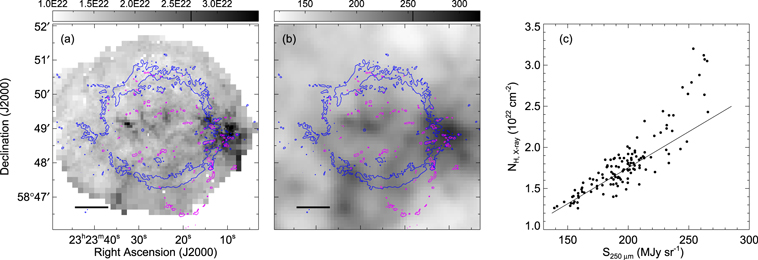
Figure 5. (a) Column density map of H nuclei from X-ray (NH,X-ray; Hwang & Laming 2012). The scale bar is in units of cm−2. The locations of QSFs are marked by magenta contours. The blue contour represents the main ejecta shell. (b) Herschel image of 250 μm brightness (S250 μm). The scale bar is in units of MJy sr−1. (c) NH,X-ray vs. S250 μm toward QSFs. The solid line shows the relation for dust emission at Td = 20 K (see the text).
Download figure:
Standard image High-resolution image5. QSF in [Fe ii] Emission
5.1. QSF Finding Chart and Their Optical Counterparts
Figure 6 is the finding chart of 130 QSFs in Table 1. The QSFs with their radial velocities known from optical observations by Alarie et al. (2014) are filled with colors based on their radial velocities. We have searched for optical counterparts of QSFs by directly comparing the deep [Fe ii]+[Si i] image with the [N ii] λ6583 line image of Alarie et al. (2014) via visual inspection instead of cross-correlating the two catalogs because QSFs in the two images have different, irregular shapes. For those with counterparts, we present the IDs and radial velocities of Alarie et al. (2014) in Table 2. Some QSFs have subknot structures in the [N ii] λ6583 image; in this case, we present the mean velocity of the subknots. Note that the QSFs in the western area are not covered in the [N ii] λ6583 image. Among the 130 QSFs, 39 are found to have optical counterparts. In some cases, two QSFs correspond to one [N ii] knot, so that about 80% of the 44 [N ii] knots in the catalog of Alarie et al. (2014) are detected in [Fe ii] emission. The other 20% of the [N ii] knots are either faint or disappeared. Several knots clearly appear to have disappeared, e.g., A6, A26, A30, and A32 in their catalog. The [N ii] image was obtained in 2009 September and 2011 December (Alarie et al. 2014), so this fraction appears rather high compared to their lifetime (≳60 yr; see below). But considering the nonuniform spatial distribution and the short time interval, this may not be statistically significant.
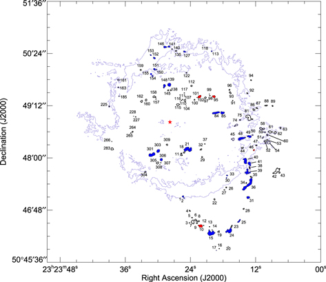
Figure 6. Finding chart of QSFs in Table 1. The filled symbols with blue and red colors represent QSFs previously detected in the [N ii] λ6583 line and with negative and positive radial velocities, respectively (Alarie et al. 2014). The background blue contour is to show the main ejecta shell in the deep [Fe ii]+[Si i] image, and it is at 4 × 10⁻¹⁸ erg cm−2 s−1 pixel−1. The red star represents the explosion center.
Download figure:
Standard image High-resolution imageIn Table 2, we also present the ID, proper motion, and radial velocity for the QSFs detected by van den Bergh & Kamper (1985, their Table 2) in Hα+[N ii] emission. We compared the deep [Fe ii]+[Si i] image with Figure 4 of van den Bergh & Kamper (1985) and Figure 7 of van den Bergh & Kamper (1983). These images had been obtained in 1983 and 1976, respectively. (Five QSFs in the southernmost area, i.e., R36–R40 in van den Bergh & Kamper 1985, are shown in the latter figure.) In the case that a [Fe ii] knot is matched with several optical knots, we present the mean values of proper motion and radial velocity. Three of the QSFs detected by van den Bergh & Kamper (1985) were not detected by Alarie et al. (2014), so that the total number of QSFs with optical counterparts is 42. The remaining 88 (=130–42) QSFs in Table 1 are new QSFs identified in this work. They are the ones surrounded by empty contours in Figure 6. About 30% of them are located in the disrupted western portion of the main ejecta shell, where the extinction is large (AV ≥ 10 mag), and most of them might have been unseen in previous optical observations because of large extinction. The faint ones could have also been undetected previously because of low sensitivity. On the other hand, there are bright, newly detected QSFs, and they might have appeared between 2011 December and 2013 September. For example, the bright Knot 7 and the surrounding knots are not seen in either Alarie et al. (2014) or van den Bergh & Kamper (1983) (see Section 5.3). It is worthwhile to note that many newly detected knots in the northeastern central region appear to be lying on an arc structure that connects to the prominent QSF arc structure in the south.
Table 2. QSFs with Optical Counterparts
| Alarie et al. (2014) | van den Bergh & Kamper (1985) | |||||||
|---|---|---|---|---|---|---|---|---|
| ID | α(J2000) | δ(J2000) | IDopt | vr | vr,err | IDopt | μ | vr |
| (km s−1) | (km s−1) | (arcsec yr−1) | (km s−1) | |||||
| (1) | (2) | (3) | (4) | (5) | (6) | (7) | (8) | (9) |
| 1a | 23:23:25.362 | 58:47:07.47 | A13 | −35 | 10 | R34 | 0.01 | ⋯ |
| 2a | 23:23:25.165 | 58:47:05.42 | A13 | −35 | 10 | R34 | 0.01 | ⋯ |
| 10 | 23:23:22.124 | 58:46:26.73 | A37 | 107 | 13 | R36n, s | 0.04 | ⋯ |
| 15 | 23:23:20.210 | 58:46:16.89 | A2 | −53 | 9 | ⋯ | ⋯ | ⋯ |
| 16 | 23:23:18.688 | 58:45:55.48 | ⋯ | ⋯ | ⋯ | R40 | 0.02 | ⋯ |
| 17 | 23:23:19.213 | 58:45:53.03 | A1 | −54 | 9 | R40 | 0.02 | ⋯ |
| 21 | 23:23:25.027 | 58:48:12.10 | A31 | −448b | 13 | R1c, e, w | 0.02 | 432 |
| 24 | 23:23:16.766 | 58:46:19.15 | A3 | −53 | 2 | R37n, s | 0.04 | ⋯ |
| 25 | 23:23:15.011 | 58:46:33.56 | A5 | −48 | 8 | R38 | 0.08 | ⋯ |
| 30a | 23:23:17.328 | 58:47:33.00 | A10 | −93 | 2 | R9c, s | 0.02 | −128 |
| 31 | 23:23:13.333 | 58:47:05.97 | A39 | −171 | 37 | ⋯ | ⋯ | ⋯ |
| 33a | 23:23:17.230 | 58:47:36.41 | A10 | −93 | 2 | R9n | 0.01 | −198 |
| 36 | 23:23:13.338 | 58:47:23.89 | A7 | −25b | 8 | ⋯ | ⋯ | ⋯ |
| 39a | 23:23:13.473 | 58:47:41.08 | A8 | −6b | 10 | R20 | 0.02 | ⋯ |
| 40a | 23:23:13.856 | 58:47:56.51 | A9 | −105b | 29 | R21 | 0.02 | ⋯ |
| 41a | 23:23:13.089 | 58:47:52.57 | A41 | −35 | 28 | ⋯ | ⋯ | ⋯ |
| 46a | 23:23:12.264 | 58:48:11.41 | A11 | 11 | 12 | R35 | 0.17 | ⋯ |
| 48a | 23:23:14.574 | 58:48:27.39 | A12 | −180b | 7 | R19 | 0.01 | −182 |
| 49a | 23:23:13.111 | 58:48:30.15 | A38 | −295 | 21 | R19 | 0.01 | −182 |
| 84 | 23:23:19.274 | 58:49:02.83 | A29 | −175 | 17 | R23 | 0.03 | ⋯ |
| 85 | 23:23:18.074 | 58:49:02.80 | A44 | −280 | 18 | R23 | 0.03 | ⋯ |
| 95 | 23:23:19.645 | 58:49:25.25 | A15 | 70 | 13 | ⋯ | ⋯ | ⋯ |
| 102 | 23:23:22.308 | 58:49:25.10 | A36 | 6 | 22 | ⋯ | ⋯ | ⋯ |
| 112 | 23:23:23.784 | 58:49:39.98 | ⋯ | ⋯ | ⋯ | (R14) | 0.17 | −340 |
| 113a | 23:23:20.057 | 58:50:27.70 | A28 | −161 | 16 | ⋯ | ⋯ | ⋯ |
| 118a | 23:23:21.677 | 58:50:35.46 | A27 | −7 | 7 | R11, R12 | 0.02 | −134 |
| 127a | 23:23:25.075 | 58:50:27.36 | A33 | −368 | 24 | R17 | 0.02 | −283 |
| 139 | 23:23:27.895 | 58:49:41.56 | A18 | −137 | 2 | R2n, s | 0.02 | −208 |
| 141a | 23:23:27.963 | 58:50:34.17 | A25 | −50 | 4 | R10 | 0.02 | −20 |
| 146a | 23:23:28.687 | 58:50:33.62 | A25 | −50 | 4 | R29e | 0.01 | −45 |
| 148 | 23:23:28.808 | 58:49:39.83 | A17 | −99 | 3 | R3 | 0.01 | −163 |
| 150a | 23:23:30.271 | 58:50:02.34 | A23 | −283 | 10 | ⋯ | ⋯ | ⋯ |
| 151a | 23:23:30.635 | 58:50:02.89 | A23 | −283 | 10 | ⋯ | ⋯ | ⋯ |
| 152a | 23:23:30.664 | 58:50:18.40 | A22 | −18 | 2 | R7n, s | 0.01 | −66 |
| 153a | 23:23:31.325 | 58:50:22.52 | A24 | −140 | 18 | R26 | 0.04 | ⋯ |
| 154a | 23:23:31.012 | 58:49:53.83 | A19 | −164 | 3 | R5e, w | 0.02 | −265 |
| 155a | 23:23:31.265 | 58:49:56.38 | A19 | −164 | 3 | ⋯ | ⋯ | ⋯ |
| 161a | 23:23:37.291 | 58:49:48.03 | A40 | ⋯ | ⋯ | R28 | 0.02 | ⋯ |
| 225a | 23:23:39.000 | 58:49:11.71 | ⋯ | ⋯ | ⋯ | R13 | 0.00 | −170 |
| 301 | 23:23:31.102 | 58:48:05.07 | A16 | −193 | 6 | R4c, e | 0.02 | −162 |
| 303 | 23:23:29.942 | 58:48:10.20 | A35 | −220 | 58 | R4w | 0.01 | −170 |
| 306 | 23:23:29.374 | 58:47:58.31 | A34 | −255 | 31 | R25 | 0.02 | ⋯ |
Notes. Column (1): knot ID. Columns (2)–(3): central coordinate from ellipse fitting. Columns (4)–(6): optical QSF ID and radial velocity with error from Alarie et al. (2014). Columns (7)–(9): optical QSF ID, proper motion, and radial velocity from van den Bergh & Kamper (1985)—if several optical QSFs are matched with an [Fe ii] knot, we use their mean proper motion and velocity. Knot 112: van den Bergh & Kamper (1985) obtained a large proper motion and put parentheses on the ID, i.e., "(R14)," to indicate a need for confirmation. But the large proper motion is likely due to confusion with another fragment in the area. The proper motion we estimate by comparing with the 2008 image is 002 yr−1.
Download table as: ASCIITypeset image
Most of the 42 QSFs in Table 2 seem to have been quite long-lived. We could not confirm the presence of all 42 QSFs in old plates because of their lower sensitivity. Instead, we checked whether the QSFs identified in previous studies are still visible in our 2013 image. Baade & Minkowski (1954) presented a broadband red plate taken in 1951, where they identified two (#2 and #3) bright QSF features. They correspond to QSF 141/146 and 301/303 in our catalog. There are also about dozen faint knot features in the image, and only one of them has disappeared. Van den Bergh (1971) presented a catalog of 19 QSFs marked on a broadband red plate taken in 1968. (They are R1–R19 in van den Bergh & Kamper 1985.) Three of them (R6, R15, and R16) are not visible in our image. (Two knots, R8 and R18, are superposed on the shell and not clear.) Van den Bergh & Kamper (1985) presented a catalog of 40 QSFs marked on a 1983 image. Three of them (R15, R31, R32) are seen neither in our deep [Fe ii]+[Si i] image nor in the 2009/2011 image of Alarie et al. (2014). One knot (R31/A32) is seen in Alarie et al. (2014) but not in our image. Van den Bergh & Kamper (1985) compared deep broadband red plates (Hα+[N ii]) taken in 1958 and 1983 and found that only 1 of 25 QSFs seen on the 1958 plate disappeared, and they concluded that most QSFs have lifetimes ≳25 yr. Our comparison above shows that the lifetimes of QSFs are indeed significantly longer than this, e.g., ≳60 yr (see also Section 5.2).
5.2. Physical Properties of QSFs
In Figure 1, QSFs are marked by magenta contours, and we can see that the bright knot features in the deep [Fe ii]+[Si i] image are mostly QSFs. This is shown quantitatively in Figure 7(a), which shows the observed [Fe ii] 1.644 μm flux distribution of the identified knots. The filled bars represent QSFs in Table 1, while the open ones are FMKs. The median of the observed fluxes (Fobs) of QSFs is 1.86 × 10⁻¹⁵ erg cm−2 s−1. For comparison, the median Fobs of the FMKs is 0.24 × 10⁻¹⁵ erg cm−2 s−1. The QSF knots are also generally large. Their geometrical mean radius is in the range of 028–439 with a median of 103 (cf. 061 for FMKs). The large fluxes of the QSFs, however, are not entirely due to their large areas as we see in Figure 7(b). The median surface brightness of QSFs is 4.21 × 10⁻¹⁶ erg cm−2 s−1 arcsec−2. Table 3 summarizes the [Fe ii] parameters of QSFs.
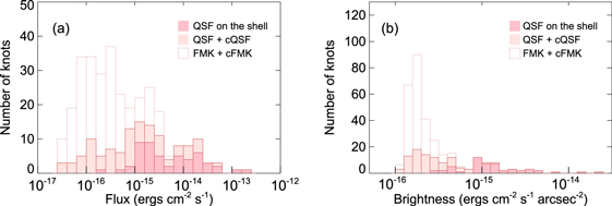
Figure 7. Distribution of (a) observed flux and (b) brightness of knots identified in the deep [Fe ii]+[Si i] image.
Download figure:
Standard image High-resolution imageTable 3. [Fe ii] 1.644 μm Properties of QSFs and FMKs
| Parameter | QSF | FMK |
|---|---|---|
| Number of identified knotsa | 130 | 179 |
| Geometrical radius (arcsec) | 1.03 (0.28–4.39) | 0.61 (0.28–2.18) |
| Dmin/Dmax | 0.70 (0.21–0.98) | 0.72 (0.14–1.00) |
| Observed | ||
| Flux (10−15 erg cm−2 s−1) | 1.86 (0.044–239) | 0.24 (0.039–5.23) |
| Brightness (10−16 erg cm−2 s−1 arcsec−2) | 4.21 (1.36–245) | 2.08 (1.35–6.38) |
| Total flux (10−12 erg cm−2 s−1) | 1.27 | 0.11 |
| Extinction corrected | ||
| Flux (10−15 erg cm−2 s−1) | 9.12 (0.14–1125) | 1.08 (0.12–22.1) |
| Brightness (10−16 erg cm−2 s−1 arcsec−2) | 20.5 (4.51–1188) | 8.94 (4.85–26.0) |
| Total flux (10−12 erg cm−2 s−1) | 7.47 | 0.46 |
| Luminosity (L⊙) | 2.70 | 0.17 |
Note. The quoted values are the median, and the numbers in parentheses are the minimum and maximum.
aThese numbers include 36 candidates for QSF and 12 candidates for FMKs. See Section 4.2 for an explanation of candidates.Download table as: ASCIITypeset image
QSFs are dense shocked clumps, and, as we discussed in Section 3.1, their 1.64 μm emission should be almost entirely due to the [Fe ii] line. In radiative atomic shocks, [Fe ii] line brightness is roughly proportional to  , where n0 is pre-shock density and vs is shock speed (see, e.g., Figure 6 of Koo et al. 2016). If the shocks propagating into the QSFs are driven by hot gas at constant ram pressure
  , then the [Fe ii] brightness of QSFs is expected to increase with vs up to
  km s−1, at which the cooling time becomes comparable to the age of Cas A (see, e.g., Equation (36.33) of Draine 2011). McKee & Cowie (1975) visually examined the brightnesses of QSFs in the Hα image of van den Bergh (1971) and claimed that indeed the QSFs with largest shock speeds are fainter. According to our result, however, there is no correlation between the [Fe ii] brightness and radial velocity of QSFs. In Figure 8, we plot extinction-corrected [Fe ii] surface brightness versus radial velocity (vrad) of QSFs for those with radial velocities known from optical observations (Alarie et al. 2014). For example, the QSFs with the highest radial velocities (vrad ≲ −350 km s−1 or vrad ≳ +100 km s−1) are not fainter or brighter than the other QSFs. Instead, the radial velocities of the brightest QSFs are ∼−100 km s−1. It has been known that QSFs are systematically blueshifted (van den Bergh & Kamper 1985; Lawrence et al. 1995; Alarie et al. 2014). The [Fe ii] line flux-weighted mean radial velocity is −120 km s−1. It is possible that this velocity represents a systemic motion of QSF knots, but the subtraction of such systemic velocity does not improve the correlation.

Figure 8. [Fe ii] 1.644 μm brightness vs. observed radial velocity for QSFs with known radial velocities. The radial velocities are from Alarie et al. (2014). QSFs are labeled by their IDs in this paper (see Figure 6). The QSFs labeled in blue are the ones on the main shell. The red solid lines show the brightness from shock models for shock speeds equal to  . The lower and upper curves are for constant ram pressure of
  and 107 cm−3 (km s−1)2, respectively. See the Appendix for the other shock parameters.
Download figure:
Standard image High-resolution imageA difficulty in examining Figure 8 is the projection effect. We may simply assume that the shocks propagating into QSFs are mainly in the radial direction from the SNR geometrical center, in which case the observed radial velocities would be the line-of-sight component of the total speed of a shock. McKee & Cowie (1975) derived the total shock speeds of individual QSFs assuming that QSFs are located near the forward shock front. This was justifiable because at that time the thickness of the region (ΔRs) between the ambient and reverse shocks was thought to be 10%–15% of the SNR radius; since QSFs are likely to be quickly destroyed once swept up by the dense shocked ejecta, they may be assumed to be in the region between the ambient and reverse shocks. We now have a better estimate for ΔRs, and it is a considerable fraction of the distance to the SNR radius (Rs), i.e., ΔRs/Rs ≈ (2.5 pc–1.7 pc)/2.5 pc = 0.32 (Reed et al. 1995; Gotthelf et al. 2001). So the QSFs that we see can spend ∼100 yr, or the corresponding fraction of the SNR age, embedded in the region of hot, shocked gas (see, e.g., Figure 10 of Nozawa et al. 2010). For comparison, the disruption timescale for a dense clump of radius a by a shock wave of speed vs is  (McKee & Cowie 1975). So QSFs with radius larger than ∼0.005 pc are likely to survive until they encounter the ejecta shell, where they will be destroyed. Since 0.005 pc is 1/3 of the median radius of QSFs, although the initial radii of QSFs could be significantly less than their observed radii, we may consider that the QSFs that we see will mostly survive until they encounter the ejecta shell and that their lifetime is ∼100 yr or even longer considering the time that they spend in the ejecta shell. This is consistent with our conclusion in Section 5.1 that the lifetime of QSFs is ≳60 yr. Therefore, in principle the QSFs outside the reverse shock can be anywhere along the line of sight and the correction factor for the projection can be very large. For example, the bright QSFs with small radial velocities, e.g., Knots 33, 30, and 40 in Figure 8, might be moving almost perpendicularly on the plane of sky, although they could be bright because they are interacting with shocked SN ejecta (see below). For the QSFs inside the reverse shock, one can derive the lower and upper limits to shock speeds, but, considering the complex structure of shocked clumps, these limits will be also quite uncertain.
In Figure 8, the red solid lines show the expected [Fe ii] brightness for shocks of constant ram pressure of 106 and 107 cm−3 (km s−1)2. The ambient shock in Cas A is probably expanding into CSM with n(r) ∝ r−2 density distribution, and the pre-shock density at the current location of the shock front is about 1 cm−3 (Lee et al. 2014b). The shock speed is about 5000 km s−1, so the thermal pressure just behind the ambient shock is  (km s−1)2. The pressure drops behind the shock front (e.g., Chevalier 1982), so the pressure driving a shock into QSFs in the shocked ambient medium will be somewhat lower, e.g., ∼2 × 107 cm−3 (km s−1)2. Figure 8 shows that most QSFs are fainter than predicted by shock models by an order of magnitude, except the ones on the main ejecta shell. We attribute this to the small area-filling factor of the [Fe ii] emitting region in QSFs. The morphology of clumps disrupted by blast waves seen in numerical simulations is quite complex (e.g., Klein et al. 1994). The HST images also show the filamentary and clumpy structure of QSFs (Alarie et al. 2014). The [Fe ii] emission is likely to be emitted from such dense filaments/fragments filling a small fraction of the QSFs' geometrical areas in Table 1. The lack of correlation between the [Fe ii] brightness and vrad could also be due to the complex spatial and kinematic structure of QSFs. The shocks are probably propagating into QSFs in all directions, and the observed radial velocities might be intensity-weighted averages of their line-of-sight velocity components. In some QSFs, the radial velocity varies more than 100 km s−1 over the structure. Therefore, the radial velocities cannot be a good tracer of shock speeds. One thing to notice in Figure 8 is that the QSFs on the main ejecta shell are relatively bright, e.g., Knots 33, 30, 40, 48, and 1. This is not just because we used a higher threshold for the detection (see Section 4.3) since there are no bright (≥10−14 erg cm−2 s−1 sr−1) QSFs detected outside the main ejecta shell. We suggest that this is because those QSFs are indeed physically interacting with the main ejecta shell; when QSFs are swept up by a dense ejecta shell, a strong shock will be driven into QSFs by the shell's large ram pressure, so that they will be brighter. A detailed spectral mapping of individual QSFs can be helpful to understand how the [Fe ii] brightness is related to their physical properties.
We can derive the total mass of Fe atoms (M(Fe)) from the [Fe ii] 1.644 μm luminosity (L[Fe ii]1.644) by
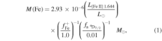
where  is the fraction of Fe in Fe+ and
  is the fraction of Fe+ in the level a4D7/2. We used Einstein coefficient A21(=5.07 × 10⁻³ s−1) of Deb & Hibbert (2011) and the collision strength of Ramsbottom et al. (2007). In statistical equilibrium,
  at temperatures 5000–10,000 K and electron density 1 × 104 cm−3. A median electron density of QSFs is a few × 104 cm−3 (Lee et al. 2017), and the characteristic temperature of the [Fe ii] 1.644 μm line emitting region is T = 7000 K (Koo et al. 2016). Hence, we may take
  . The total [Fe ii] 1.644 μm flux of QSF knots is 7.47 × 10⁻¹² erg cm−2 s−1, so that L[Fe ii]1.644 = 2.70 L⊙ (Table 2). This implies M(Fe) ≈ 7.9 × 10⁻⁶ M⊙, and for the cosmic abundance of Fe, i.e., X(Fe) = 3.5 × 10⁻⁵, hydrogen+helium mass M(H + He) ≈ 0.23 M⊙. For comparison, van den Bergh (1971) obtained 0.025 M⊙ from their Hα flux applying an extinction correction factor of 100. If we consider that the extinction to Cas A is AV = 6–11 mag and that the QSFs in the western area that contribute ≳60% of the total [Fe ii] line flux (see below) are not seen in Hα, the two estimates roughly agree with each other. For comparison, the total mass of the X-ray-emitting swept-up material, representing the smooth red supergiant (RSG) wind, is ∼6 M⊙ (Lee et al. 2014b). Hence, according to our result, the mass of visible QSFs is about 4% of the total swept-up wind mass. If we naively scale the observed mass using the ratio of the total volume of the SNR to the volume of the region between ambient and reverse shocks (see Section 5.2), the fraction becomes a little larger (∼6%).
5.3. QSFs and Mass-loss History of the Cas A Progenitor
Figure 6 shows some distinct features of the spatial distribution of QSFs. The most prominent one is the arc structure in the south (hereafter the "southern QSF arc"), which had been noticed by previous studies in Hα+[N ii] images. Lawrence et al. (1995) noticed that QSFs along this arc structure, together with the QSF knots in the northern area, are located along the edges of a 47 × 23 ellipse with a P.A. of 25°. They noted that this QSF distribution, however, cannot be an inclined circle or an ellipse centered at the expansion center because all QSFs have velocities between −100 and −200 km s−1 and because there is no correlation between radial velocities and the P.A. The southern QSF arc is also prominent in the [N ii] λ6583 image of Alarie et al. (2014). The measured velocities cover a wider range, e.g., +110 to −180 km s−1, but show no systematic variation (see Figure 6).
The QSFs along the southern QSF arc seem to have appeared over some considerable period of time. Van den Bergh & Kamper (1983) and van den Bergh & Kamper (1985) were the first to identify QSFs in this area: Knots 10, 17, 24, and 25 (=R36, R40, R37, and R38 in van den Bergh & Kamper 1985; see Figure 9).8 For the bright Knot 24 (=R37), they noted that it can be seen in all available plates from 1951 to 1980. Hence, this QSF had appeared before 1951 and has been visible during ≳62 yr including our deep [Fe ii]+[Si i] image. For Knot 10 (=R36), they noted that it had been invisible until 1958 and marginally visible in 1965 and clearly seen on all plates taken since 1967. In a recent Hα+[N ii] image shown in Figure 9, we can confirm these QSFs. The Hα+[N ii] image in Figure 9 has been produced from the Isaac Newton Telescope (INT) Wide Field Survey (WFS) data obtained in 2005 October.9 On the other hand, we note that Knot 7 in our image is not visible in any of the previously published Hα+[N ii] images, including the 2009 [N ii] image of Alarie et al. (2014) (see also Figure 9), so that this bright knot (and possibly the surrounding faint knots too) appeared after 2009. If we assume that the moment that they appear is the moment that these dense knots are swept up by the SNR shock, then Knot 7 might be slightly farther away, e.g., by ∼0.3 pc using the SNR shock speed of 5000 km s−1, from the SNR center than Knot 24, although the former appears closer on the sky. And the knots along the southern QSF arc, together with the QSF knots in the northern area that Lawrence et al. (1995) noticed, are likely distributed along an elliptical ring, but they appear as they are because of projection. The fact that these knots are systematically blueshifted suggests that the elliptical ring is likely located on the near side of the SNR shock.

Figure 9. Left: enlarged view of the southern QSF arc. QSFs are marked by magenta contours and labeled by their IDs in Table 1 (see also Figure 6). The green contour marks the outer boundary of the SNR in radio. Right: same as the left panel, but in Hα+[N ii] emission. The image has been produced from the INT WFS data obtained in 2005 October, and a continuum is subtracted by using an r' broadband image. QSFs identified in optical emission are labeled by their IDs in the catalogs of Alarie et al. (2014) and van den Bergh & Kamper (1985) (see Table 2).
Download figure:
Standard image High-resolution imageFigure 6 reveals another prominent feature, namely, the cluster of QSFs in the western area beyond the main ejecta shell. Figure 10 shows the spatial and flux distribution of QSFs as a function of P.A. measured from north to east with respect to the explosion center. It shows that QSFs are concentrated in the southwestern area near P.A. ∼ 260° or toward the direction of the SW counterjet. The QSFs between P.A. = 240° and 280° contribute ≳60% of the extinction-corrected flux of QSFs. The median value of their proper motions is 002 yr−1, which gives an expansion timescale of ∼6000 yr but with a large uncertainty (±6000 yr) due to our short time interval. For comparison, the expansion timescale of QSFs from optical studies is 11,000 ± 2000 yr (Kamper & van den Bergh 1976; van den Bergh & Kamper 1985). The expansion timescale, however, could be longer if the observed proper motion is partly due to shock motion into QSFs (see below). Therefore, if the QSFs that we see were ejected during a short time interval, Figure 10 suggests that there was an eruptive mass loss ≳10,000 yr ago, mainly to the west.
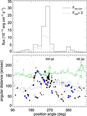
Figure 10. Top: fluxes of QSFs vs. their position angle (P.A.). The P.A. is measured from north to east with respect to the explosion center, so the west, for example, corresponds to P.A. = 270°. The dotted histogram shows the distribution of observed fluxes multiplied by three, while the solid histogram shows the distribution of extinction-corrected fluxes. Bottom: angular distance of QSFs measured from the explosion center vs. their P.A. Filled circles represent the locations of QSFs. The area of the symbols is proportional to the QSF flux, while the color of the symbols represents the QSF velocities, i.e., blue = negative velocities, red = positive velocities, and black = unknown velocities. The gray contour shows the location of the main ejecta shell.
Download figure:
Standard image High-resolution imageIt has been suggested that QSFs are dense clumps embedded in a smooth RSG wind from the Cas A progenitor (Chevalier & Oishi 2003). High-resolution studies of nearby RSGs indeed reveal inhomogeneities indicating anisotropic and episodic mass ejection (Mauron 1997; de Wit et al. 2008; Ohnaka 2017). But we note that the proper motion (002 yr−1) of QSFs corresponds to 320 km s−1, which is much greater than the typical expansion speed of RSG wind, i.e., ∼15 km s−1 (Mauron & Josselin 2011). Therefore, if QSFs are dense clumps in RSG wind, the observed proper motion (and radial velocities) should be almost entirely due to the shock motion, and the expansion timescale for the QSFs needs to be ≲(2.5 pc)/(15 km s−1) ∼ 1.6 × 10⁵ yr. Based on stellar evolution models, Yoon & Cantiello (2010) suggest that, at about this time before the SN explosion, RSG stars with initial mass of ≳17 M⊙ have a brief period of "superwind" phase where the star experiences strong H envelope pulsation with an order-of-magnitude enhanced mass-loss rate. The mass ejection could have been asymmetric if a nonradial mode of pulsation was dominant. On the other hand, if the progenitor was in a binary system, a dense and clumpy spiral structure can be formed in the equatorial plane by wind−wind interaction (see, e.g., Figure 1 of Pan et al. 2015), which will become a circular or an elliptical arc at a distance of ≳1 pc from the explosion center at the time of SN explosion. If the arc is inclined, it may appear as the southern QSF arc. Lawrence et al. (1995) ruled out such a possibility because all QSFs have negative velocities and there is no correlation between the radial velocity and P.A.. But if the progenitor system was moving through the interstellar space at ∼−100 km s−1 and the velocity structures of individual QSFs are dominated by shocks, then it does not seem to be impossible to see the observed velocity distribution of QSFs.
Another possible explanation for QSFs is that they are dense clumps ejected in the common envelope phase of the progenitor binary system. The small ejecta mass, together with N-rich CSM, suggests that the progenitor was an He star in a binary system (Young et al. 2006). The nondetection of the ex-companion implies that the companion star could have been either a white dwarf or a neutron star (Kerzendorf et al. 2017). A plausible evolutionary scenario for such a system is that the progenitor in the late RSG phase expands and forms a common envelope through the Case C mass transfer to the companion. Then there could be a brief and explosive mass loss in the common envelope phase. For example, the outburst of a "luminous red nova (LRN)" is considered to be the mass loss from a binary system in its common envelope phase (Ivanova et al. 2013). The characteristic expansion velocities of the LRN outburst are 200–1000 km s−1 (Ivanova et al. 2013, and references therein), so that the dense clumps ejected during the outburst will propagate ballistically through the slow (∼15 km s−1) RSG wind because of large density contrast. The "large" proper motion (320 km s−1) of QSFs can be explained by such an outburst and their systematic blueshift by one-sided ejection toward us, although there seems to be no plausible explanation for such highly asymmetric ejection.
6. FMKs and Shocked Dense SN Ejecta
6.1. FMKs outside the Main Ejecta Shell
We have identified 179 FMKs outside the main ejecta shell (Table 1). Their measured proper motions range from 018 to 076 yr−1, with a median of 049 yr−1 or 7900 km s−1. They are mostly found in four regions: (1) NE jet, (2) southeastern area of P.A. = 80°–150°, (3) SW counterjet, and (4) northern area of P.A. = 320°–5°. (see Figure 1). No FMKs are found in broad regions between these areas. That spatial distribution is similar to the distribution of optical ejecta knots reported by Fesen et al. (2006a) and Hammell & Fesen (2008). From the HST observations in various filters, 1825 outlying optical ejecta knots have been found, and they are divided into N-rich, O-rich, and S-rich knots (Hammell & Fesen 2008). These chemically distinct ejecta knots show very different spatial distributions: N-rich knots are arranged in a broad shell with gaps in the north and south; O-rich knots, which are fewer in number, are found in limited P.A. and radial distance ranges; and S-rich knots are mainly concentrated in the NE jet, the SW counterjet, and the southeastern area (Fesen et al. 2006a; Hammell & Fesen 2008; see also Milisavljevic & Fesen 2013 and Fesen & Milisavljevic 2016). The FMKs in the deep [Fe ii]+[Si i] image are mostly S-rich knots: among the 128 outlying FMKs located in the area covered by Hammell & Fesen (2008),10
6 (5%), 2 (2%), and 93 (73%) knots are N-rich, O-rich, and S-rich ejecta knots in the catalog of Hammell & Fesen (2008), respectively. Twenty-seven (21%) FMKs do not have counterparts in the catalog of Hammell & Fesen (2008). In Figure 11, we show the deep [Fe ii]+[Si i] image of the NE jet area, southeastern area, and SW jet area together with the HST F098M image. The HST F098M image was obtained in 2011 November 18 (Fesen & Milisavljevic 2016), 1.9 yr earlier than the deep [Fe ii]+[Si i] image, and the FMK contours are shifted considering their proper motions. We can see that essentially all FMKs have counterparts in the HST image, including the ones without counterparts in the catalog of Hammell & Fesen (2008). (The HST F098M image has a higher sensitivity than the HST F850LP used by Hammell & Fesen 2008.) N-rich knots of Hammell & Fesen (2008) are marked by plus signs, and only a few N-rich knots have counterparts in our deep [Fe ii]+[Si i] image. In particular, in the southeastern area, there are numerous N-rich knots, but none of them have counterparts in [Fe ii] emission. Some knots could have been missed because of our narrow bandwidth (±2600 km s−1), but according to spectroscopic observations (Fesen 2001), N-rich knots with radial velocities outside our band are expected to be rare in this area. Therefore, we tentatively conclude that most FMKs in the deep [Fe ii]+[Si i] image, including the ones not cataloged by Hammell & Fesen (2008), are S-rich optical ejecta knots.
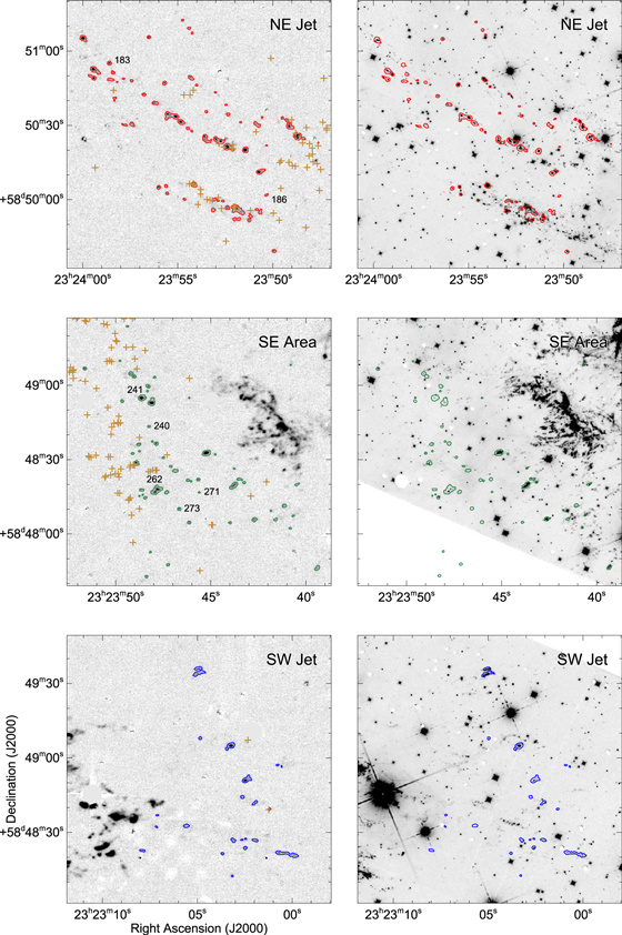
Figure 11. Enlarged view of NE jet, SE area, and SW counterjet in the deep [Fe ii]+[Si i] image (left) and in the HST F098M image (right). The contours in the deep [Fe ii]+[Si i] image mark the identified FMKs, while those in the HST F098M image are the same contours but shifted to the position at the epoch (2011 November) of the HST image by assuming that the FMKs have been freely expanding from the explosion center since A.D. 1670. FMKs with ![${F}_{{\rm{F}}098{\rm{M}}}/{F}_{[\mathrm{Fe}{\rm{II}}]1.644\mu {\rm{m}}}\leqslant 0.3$](https://content.cld.iop.org/journals/0004-637X/866/2/139/revision1/apjaae20eieqn17.gif) in Figure 12 are labeled by their IDs. The brown plus signs mark the positions of N-rich optical ejecta knots in the catalog of Hammell & Fesen (2008).
in Figure 12 are labeled by their IDs. The brown plus signs mark the positions of N-rich optical ejecta knots in the catalog of Hammell & Fesen (2008).
Download figure:
Standard image High-resolution imageIn Figure 11, we notice that the outer FMKs in the southeastern area, e.g., Knots 240, 241, 262, 271, and 273, are generally brighter in the deep [Fe ii]+[Si i] image than in the HST F098M image. Figure 12 shows this quantitatively, where we plot the flux ratio (FF098M/F[Fe ii]1.644) of FMKs as a function of angular distance from the explosion center in three areas. The left frame is for the observed fluxes, while the right frame is for the extinction-corrected fluxes. The extinction correction raises the flux ratios systematically, but the trend remains the same. Note that F[Fe ii]1.644 is the flux within the narrow band (±2600 km s−1), so there could be missing flux compared to the broadband F098M flux. Outlying ejecta knots often show radial velocities as large as 5000 km s−1, although the majority of knots have more modest radial velocities, e.g., −3000 to +1000 km s−1 (Fesen & Gunderson 1996; Fesen 2001; Milisavljevic & Fesen 2013). With that caveat in mind, we note in Figure 12 that FMKs at angular distance ≳25 in the southeastern area (green squares) have relatively low FF098M/F[Fe ii]1.644. The missing [Fe ii] flux will shift the data points upward not downward. Hence, these knots appear to be Fe-rich, indicating that a significant fraction of Fe ejecta may have mixed out to large radius in the southeast. It is interesting that this is the area where the diffuse X-ray Fe–K emission extends beyond the main ejecta shell (Hwang et al. 2004). DeLaney et al. (2010) proposed an ejecta piston model where Fe ejecta moving faster than the average ejecta is pushing the O-burning layer above. Dense Fe-rich knots embedded in diffuse Fe-rich ejecta appear to be consistent with small-scale clumping and large-scale anisotropy seen in the recent 3D numerical simulations of neutrino-driven SN explosions (Wongwathanarat et al. 2015; Orlando et al. 2016). The line ratio derived from the two images of several years' interval, however, can be affected by the brightness changes or flickering during the interval (Fesen et al. 2011), so we need NIR spectroscopy to confirm such chemical variation of the outlying FMKs. That will be done in our forthcoming paper.
Figure 12. Left: flux ratio ![${F}_{{\rm{F}}098{\rm{M}}}/{F}_{[\mathrm{Fe}{\rm{II}}]1.644\mu {\rm{m}}}$](https://content.cld.iop.org/journals/0004-637X/866/2/139/revision1/apjaae20eieqn18.gif) of FMKs with the observed [Fe ii] 1.644 μm flux ≥5 × 10⁻¹⁷ erg cm−2 s−1 (see Figure 8) as a function of angular distance from the explosion center. Right: same as the left panel, but with the interstellar extinction corrected. FMKs with
of FMKs with the observed [Fe ii] 1.644 μm flux ≥5 × 10⁻¹⁷ erg cm−2 s−1 (see Figure 8) as a function of angular distance from the explosion center. Right: same as the left panel, but with the interstellar extinction corrected. FMKs with ![${F}_{{\rm{F}}098{\rm{M}}}/{F}_{[\mathrm{Fe}{\rm{II}}]1.644\mu {\rm{m}}}\leqslant 0.3$](https://content.cld.iop.org/journals/0004-637X/866/2/139/revision1/apjaae20eieqn19.gif) are labeled by their IDs. The 1σ uncertainties in the observed and extinction-corrected flux ratios are typically ∼4% and ∼15%, respectively.
are labeled by their IDs. The 1σ uncertainties in the observed and extinction-corrected flux ratios are typically ∼4% and ∼15%, respectively.
Download figure:
Standard image High-resolution image6.2. [Fe ii] Emission from FMKs
FMKs are shocked ejecta material, and most of the 1.64 μm emission from FMKs is probably due to the [Fe ii] 1.644 μm line (see Section 3.1). FMKs are much fainter than QSFs, e.g., by an order of magnitude in flux (Table 3). Their brightness, i.e., flux divided by the area, is also less than that of QSFs by a factor of 2–3. That is due to a tendency of the shocked ejecta to cool so quickly that much of the Fe remains in higher ionization states in the region that produces [Fe ii] emission in normal abundance shocks. The total observed and extinction-corrected fluxes of FMKs are 1.1 × 10⁻¹³ erg cm−2 s−1 and 4.6 × 10⁻¹³ erg cm−2 s−1, respectively.
There is considerable uncertainty about the fractions of various FMK emission lines that are produced in the shocked gas and the pre-shock photoionization region (Itoh 1981; Sutherland & Dopita 1995; Blair et al. 2000). Docenko & Sunyaev (2010), analyzing Spitzer and ISO maps, found that the emission from singly ionized species such as [S ii] and [Fe ii] arises mostly from the post-shock photoionized region. The densities of around 3 × 104 cm−3 obtained from the [Fe ii] lines by Koo et al. (2013) also imply that the [Fe ii] line mostly comes from the post-shock region. We note that Docenko & Sunyaev (2010) obtained a density an order of magnitude higher for the FMKs based on the [O i] FIR line ratio from ISO. One possible reason for this discrepancy may be that the [O i] lines can form in much colder gas than the [Fe ii] lines because of their low excitation potential, and the density may be higher there. Another possibility is that [Fe ii] is suppressed at the high densities where the [O i] lines are produced, so emission from intermediate densities dominates. The third, and in our view most likely, possibility is that the lines come from both pre- and post-shock gas, and their line ratios are in the low- and high-density limits, respectively. In that case, the observed ratio will apparently indicate an intermediate density, while in fact it indicates the fractions of emission from the pre-shock and post-shock gas. The fairly high densities given by the [Fe ii] line ratio indicate that most of the [Fe ii] emission is from the post-shock region, in agreement with the conclusions of Docenko & Sunyaev (2010). This also fits in with the [S ii] observations of Alarie et al. (2014), who found that the [S ii] ratio varies all the way from the low-density limit to the high-density limit, with most positions giving a value near the high-density limit.
6.3. [Fe ii] Luminosity of Shocked Dense Ejecta
The total [Fe ii] 1.644 μm luminosity of Cas A in the deep [Fe ii]+[Si i] image is 2.3 L⊙. If we apply extinction correction to each pixel of the main shell in the same way as we did for the knots, we obtain 11.8 L⊙ for the extinction-corrected [Fe ii] 1.644 μm luminosity of Cas A. The QSFs contribute 23% of this (Table 3), so that the total luminosity due to the shocked SN ejecta in Cas A is 9.1 L⊙, most of which is from the main ejecta shell. Note that this does not include the fast-moving (>2600 km s−1) ejecta undetected in our narrowband image, but their contribution should be almost negligible. For comparison, the observed [Fe ii] 1.644 μm luminosity of the Kepler SNR is 0.7 L⊙ (Oliva et al. 1989), so Cas A is much brighter than Kepler. In the Galaxy, however, there are many SNRs interacting with dense environment and very bright in [Fe ii] emission (Y.-H. Lee et al. 2018, in preparation), so that Cas A is not a particularly bright SNR in [Fe ii] emission. What makes Cas A special is that, in Cas A, the [Fe ii] emission is mostly from the shocked SN ejecta, not from the shocked circumstellar or shocked ISM.
We can estimate the total mass of Fe SN ejecta associated with the [Fe ii] emission. If we substitute the extinction-corrected luminosity (9.1 L⊙) of shocked SN ejecta in Equation (1), we obtain an Fe mass of 2.7 × 10⁻⁵ M⊙. Essentially all of this mass is in the main ejecta shell. This is in fact a lower limit because there could be neutral Fe atoms that have already cooled down. However, because the optical emission has been steadily brightening in recent decades (Patnaude & Fesen 2014), it is likely that the amount of material in shocked ejecta that have faded is small compared to the present [Fe ii] line emitting mass. There may also be some Fe in higher ionization states, and a significant fraction of Fe may remain in dust. Micelotta et al. (2016) find that only about 10% of the dust in FMKs survives, but much of the destruction occurs after the grains move from the ejecta knots into the hotter surrounding material. For comparison, the mass of diffuse, X-ray-emitting Fe ejecta has been estimated to be ∼0.1 M⊙ (Hwang & Laming 2012), while the mass of unshocked Fe ejecta in the interior inferred from the 44Ti emission is also ∼0.1 M⊙ (Grefenstette et al. 2014). Hence, the mass of dense [Fe ii] line emitting Fe ejecta appears to be only a few × 10−4 of the total Fe ejecta mass.
7. Conclusion and Summary
Cas A is one of the first SNRs detected in the optical band (Baade & Minkowski 1954; Minkowski 1959), and since then it has been a subject of extensive optical studies. Studies in the NIR band, however, have been limited. Here we present a deep [Fe ii]+[Si i] image of Cas A obtained with a narrowband filter centered at 1.644 μm emission. The image gives an unprecedented panoramic view of Cas A, showing the prominent main shell and FMKs of shocked SN ejecta, compact QSFs of shocked CSM, and faint diffuse emission from the unshocked SN ejecta in the interior, all in a single image. The emission from shocked CSM and probably that from the SN ejecta too are mostly [Fe ii] 1.644 μm emission, while the emission from the unshocked SN ejecta is likely dominated by [Si i] 1.645 μm emission. The image reveals for the first time the detailed structure of the interior diffuse emission closely related to the explosion dynamics and that of the western portion of the main ejecta shell disrupted by the jet. The image also shows a comprehensive sample of QSFs that can be used to infer the mass-loss history of the progenitor system. The results presented in this paper show that the NIR band can provide new and important information about the final evolution and SN explosion of massive stars. In the following, we summarize our main results.
- (1)The deep [Fe ii]+[Si i] image shows in detail the complex structure of the diffuse emission in the interior of Cas A from the unshocked SN ejecta. Some emission features have unique morphology, implying their close association with SN explosion dynamics, e.g., the Eastern Arc surrounding the explosion center and the pillars protruding from the main ejecta shell and pointing to the explosion center. The overall morphology, however, is not correlated with 44Ti emission but well correlated with [Si ii] 34.81 μm emission, so that the emission is likely due to the [Si i] 1.645 μm line, not the [Fe ii] 1.644 μm line.
- (2)The deep [Fe ii]+[Si i] image reveals the disrupted western part of the main ejecta shell that was not visible in the optical band owing to large extinction. The area is filled with bright and faint clumps of ≲20''. The faint clumps, in general, show large proper motions over 5 yr, and they are probably the fragments of the disrupted ejecta shell. In contrast, the bright clumps in general show little proper motion, and they are probably QSFs of circumstellar origin. Some large QSFs appear to be interacting with shocked diffuse ejecta material, implying that they have been swept up by the reverse shock very recently. The possibility that the anomalous radio properties in this area could be due to the dense CSM and/or the shell fragments needs to be explored.
- (3)We have identified 309 knot features in the deep [Fe ii]+[Si i] image and derived their geometrical parameters and [Fe ii] fluxes. We classified their nature, i.e., QSF versus FMK, by comparing with another 1.64 μm image of Cas A obtained 5 yr earlier in 2008 August and also with the HST images sensitive to [S ii] lines. A total of 130 knots are classified as QSFs, and the remaining 179 knots are classified as FMKs. A catalog of 309 knots is presented in Table 1, and their characteristic [Fe ii] parameters are summarized in Table 3.
- (4)We have searched for counterparts of QSFs in Hα/[N ii] λλ6548, 6583 images published since 1951 or vice versa. Eighty-eight (68%) of 130 QSFs in the deep [Fe ii]+[Si i] image are newly identified. On the other hand, most QSFs seen in previous studies are visible in our deep [Fe ii]+[Si i] image, indicating that the lifetime of QSFs is ≳60 yr. Most QSFs are likely to survive until they encounter the ejecta shell. For QSFs with radial velocities known from optical observations, we explored whether the radial velocity can be an indicator of shock speed. We found that the [Fe ii] 1.644 μm brightness is not correlated with the radial velocity and that it is much lower than what shock models predict. We attribute this to the complex spatial and velocity structure of QSFs.
- (5)The total H+He mass of visible QSFs is estimated to be ≈0.23 M⊙, which corresponds to 4% of the total mass of the swept-up CSM. The fraction of dense clumps in the RSG wind could be a little larger (6%) if we consider the finite lifetime of QSFs. The spatial distribution of QSFs is highly asymmetric. In addition to the prominent southern arc known from optical observations, the deep [Fe ii]+[Si i] image revealed a cluster of QSFs in the western area, contributing more than 60% of the total flux. The QSF distribution indicates that the progenitor system ejected its envelope eruptively to the west just before the explosion, i.e., 104–105 yr before the explosion depending on whether these QSFs are ejected at ∼15 km s−1 in RSG phase or ejected at a few × 102 km s−1 in common envelope phase of the progenitor binary system.
- (6)We have identified 179 FMKs outside the main ejecta shell in the deep [Fe ii]+[Si i] image. FMKs are generally much fainter than QSFs in [Fe ii] emission. Most of these FMKs are S-rich optical ejecta knots, and we can identify the counterparts of essentially all FMKs in the HST F098M image. We note that the FMKs outside the southeastern disrupted ejecta shell are relatively brighter in the deep [Fe ii]+[Si i] image than in the HST F098M image compared to the other FMKs. This is the area where the diffuse X-ray Fe K emission extends beyond the main ejecta shell, and the FMKs there may be Fe-rich. That needs to be confirmed from spectroscopic observations.
- (7)The total extinction-corrected [Fe ii] 1.644 μm luminosity of Cas A is 11.8 L⊙, 23% of which is from QSFs. The total Fe luminosity of shocked SN ejecta is 9.1 L⊙, and it is mostly from the main ejecta shell. The inferred [Fe ii]-emitting, dense Fe mass in the ejecta shell is 2.7 × 10⁻⁵ M⊙, which is only a few × 10−4 of the total Fe ejecta mass.
We thank the referee for highly perceptive comments, which helped us improve the discussion about QSFs and FMKs significantly. We also thank Rob Fesen for many helpful comments. This research was supported by the Basic Science Research Program through the National Research Foundation of Korea (NRF) funded by the Ministry of Science, ICT and Future Planning (2017R1A2A2A05001337).
Facilities: UKIRT - United Kingdom Infrared Telescope, Hale - , Spitzer - , HST - , INT. -
Software: IDL.
Appendix: [Si i] 1.645 μm Line from Radiative Shocks
The [Si i] 1.645 μm line is not included in most shock models, and there is little recent atomic data. Here we compute the brightness of the [Si i] line in radiative atomic shock with QSF and FMK abundances. For the collision strength of [Si i], we use the result of Pindzola et al. (1977). Because Si i is neutral, the excitation cross section goes to zero at threshold (0.781 eV = 9060 K for the 1D2 level), which means that the (velocity-averaged) collision strength is very small at temperatures below about 4000 K. For comparison, the excitation energy of the [Fe ii] 1.644 μm line is 11,400 K, but because Fe ii is an ion, the collision strength does not go to zero at threshold, and the excitation rate is higher at a few thousand kelvin. Excitation of the [Si i] 1.645 μm line requires both the presence of Si i (T < 10,000 K) and a temperature high enough to overcome the Boltzmann factor (T > 2000 K). We scale [C i] λ9850 line flux to estimate the [Si i] brightness. The [C i] λ9850 line is similar to the [Si i] 1.645 μm line in the behavior of its excitation rate with temperature and in the ionization fraction of C i. The [Si i] 1.645 μm emission could also come from recombination of the Si ii ion. The existence of Si ii at low temperatures in the post-shock layer guarantees that there will be some [Si i] emission produced by recombination. To compute the contribution of recombination to the [Si i] line, we use the recombination coefficients of Abdel-Naby et al. (2012) and assume that 1/4 of the recombinations go by way of the singlets and that all those pass through the 1D state of the ground level.
For QSFs, we adopt the solar abundances of Asplund et al. (2009) except He and N, which are assumed to be enhanced by a factor of 2. Note that the solar abundances of Si and Fe are comparable, i.e., X(Si/H) = 3.55 × 10⁻⁵ and X(Fe/H) = 3.47 × 10⁻⁵ by number, respectively. The shock code that we use is the one developed by Raymond (1979), with updated atomic parameters (Koo et al. 2016). We have run models with shock speed vs = 50–300 km s−1 and pre-shock density n0 = 102–3 × 103 cm−3, which are the characteristic parameters of QSFs (McKee & Cowie 1975; Chevalier & Oishi 2003). Magnetic field strength is fixed to 5 μG. We find that the [Si i] line is only ≤2% as strong as the [Fe ii] line in these models. This is mainly because Fe ii is the majority ion of iron in the photoionized, radiative zone in shocked gas, while Si i is a minority species there (see also Figure 6 of Koo et al. 2016). The emission from the recombination of [Si ii] ions is not significant either. Therefore, for QSFs, the 1.64 μm line should be dominated by the [Fe ii] line emission.
FMKs are oxygen-rich SN ejecta material (e.g., Fesen 2001; Morse et al. 2004; Docenko & Sunyaev 2010). The abundances of Si and Fe in FMKs are not known, and they probably vary substantially among FMKs. As a representation, we adopt an abundance set where H = [12.00], He = [11.00], C = [14.80], O = [16.00], Ne = [15.50], Mg = [14.80], Si = [14.70], S = [14.90], Ar = [14.50], Ca = [14.00], Fe = [14.70], and Ni = [14.00] in log scale. These abundances are from Morse et al. (2004) except Fe, which we set equal to the Si abundance. Note that the abundances of O, S, Ar, and Ca are constrained by optical emission lines from shocked SN ejecta in Cas A, while the abundances of the other elements are not constrained (Morse et al. 2004). We have run models with shock speed vs = 50–200 km s−1 and pre-shock density n0 = 10–102 cm−3 using the shock code developed for SN ejecta (Raymond 1979; Cox & Raymond 1985; Blair et al. 2000; Koo et al. 2013). Magnetic field strength is fixed at 5 μG. The results are shown in Figure 13, where we see that the flux ratio F[Si i]1.645/F[Fe ii]1.644 attains a maximum of 10% at vs = 100 km s−1. The ratio is less than a few percent at other velocities. Note that the result is for Si abundance equal to Fe abundance. If the Si abundance is greater than the Fe abundance by an order of magnitude, the intensity ratio can be ∼1.
Figure 13. Ratio of [Si i] 1.645 μm to [Fe ii] 1.644 μm line intensities as a function of shock speed vs. Open and filled symbols represent the cases for pre-shock ion density n0 = 10 and 100 cm−3, respectively.
Download figure:
Standard image High-resolution imageFootnotes
- 5
There is also an H Brackett line
 (1.640688 μm) in the band, but it is much weaker than the [Fe ii] 1.644 μm line in shocked atomic gas, and also most of its contribution will be removed by subtracting the H-band image.
 - 6
In an accompanying paper (Raymond et al. 2018), we explore the origin of the interior diffuse emission using NIR spectroscopic data.
- 7
The Fit_Ellipse is a part of the Coyote IDL Program Libraries (http://www.idlcoyote.com).
- 8
Van den Bergh & Kamper (1983) and van den Bergh & Kamper (1985) detected another faint knot in the southwestern corner of Figure 9. They classified this knot (R39) as QSF because it was not seen in either [S ii]- or [O iii]-sensitive plates. But later, this knot was found to have a large proper motion, i.e., 0
65 ± 010, and reclassified as an N-rich fast-moving flocculus (FMF) by Fesen et al. (1987). A faint knot matching R39 is visible in our deep [Fe ii]+[Si i] image, although it is not marked in Figure 9. - 9
The data are available at the INT WFS archive site http://apm3.ast.cam.ac.uk/cgi-bin/wfs/dqc.cgi.
- 10
The other 51 FMKs are located near the main ejecta shell, which was not explored by Hammell & Fesen (2008). For example, the northern area, where we have found 46 FMKs, was not included in their study. Note that, in this paper, the term "FMKs" refers to any fast-moving ejecta knots, while in Hammell & Fesen (2008) the term is used either for ejecta knots in the main ejecta shell or for outlying ejecta knots chemically similar to the "main-shell FMKs."
