


Abstract
We determine the thermal evolution of the intergalactic medium (IGM) over 3 Gyr of cosmic time  by comparing measurements of the Lyα forest power spectrum to a suite of ∼70 hydrodynamical simulations. We conduct Bayesian inference of IGM thermal parameters using an end-to-end forward modeling framework whereby mock spectra generated from our simulation grid are used to build a custom emulator that interpolates the power spectrum between thermal grid points. The temperature at mean density T0 rises steadily from
  at z = 5.4, peaks at 14,000 K for z ∼ 3.4, and decreases at lower redshift, reaching T0 ∼ 7000 K by z ∼ 1.8. This evolution provides conclusive evidence for photoionization heating resulting from the reionization of
  , as well as the subsequent cooling of the IGM due to the expansion of the universe after all reionization events are complete. Our results are broadly consistent with previous measurements of thermal evolution based on a variety of approaches, but the sensitivity of the power spectrum, the combination of high-precision measurements of large-scale modes (
 ) from the Baryon Oscillation Spectroscopic Survey with our recent determination of the small-scale power, our large grid of models, and our careful statistical analysis allow us to break the well-known degeneracy between the temperature at mean density T0 and the slope of the temperature–density relation γ that has plagued previous analyses. At the highest redshifts, z ≥ 5, we infer lower temperatures than expected from the standard picture of IGM thermal evolution leaving little room for additional smoothing of the Lyα forest by free streaming of warm dark matter.
Export citation and abstract BibTeX RIS
1. Introduction
The Lyman alpha (Lyα) forest (Gunn & Peterson 1965; Lynds 1971) is the premier probe of diffuse baryons in the intergalactic medium (IGM) at high redshifts. Its fluctuations can be accurately described in the current ΛCDM framework—on large scales it is mostly sensitive to cosmological parameters such as the amplitude of fluctuations σ8, primordial power spectrum slope  , baryon density Ωb, number of neutrino species Neff, and the sum of neutrino masses
  (Palanque-Delabrouille et al. 2015; Rossi 2017). On small scales, however, it is sensitive to the thermal state of the IGM.6
This alters the observed spectra via the Doppler broadening of absorption features due to thermal motions, as well as pressure smoothing of the gas (sometimes called "Jeans" broadening), which affects the underlying baryon distribution and depends on the integrated thermal history of the IGM (Gnedin & Hui 1998; Kulkarni et al. 2015; Oñorbe et al. 2017a). The thermal evolution is largely driven by impulsive heating from cosmic reionization events and the cooling process due to adiabatic expansion and Compton cooling (McQuinn & Upton Sanderbeck 2016).
(Palanque-Delabrouille et al. 2015; Rossi 2017). On small scales, however, it is sensitive to the thermal state of the IGM.6
This alters the observed spectra via the Doppler broadening of absorption features due to thermal motions, as well as pressure smoothing of the gas (sometimes called "Jeans" broadening), which affects the underlying baryon distribution and depends on the integrated thermal history of the IGM (Gnedin & Hui 1998; Kulkarni et al. 2015; Oñorbe et al. 2017a). The thermal evolution is largely driven by impulsive heating from cosmic reionization events and the cooling process due to adiabatic expansion and Compton cooling (McQuinn & Upton Sanderbeck 2016).
Current constraints imply that hydrogen and  were reionized at
  7
(see Planck Collaboration et al. 2018). Additionally, measurements of the Lyα forest optical depth show a strong increase close to z = 6, leading to complete Gunn–Peterson absorption (Fan et al. 2006; Becker et al. 2015; Bosman et al. 2018; Eilers et al. 2018), which reveals that reionization ends at z ∼ 6. As for
7
(see Planck Collaboration et al. 2018). Additionally, measurements of the Lyα forest optical depth show a strong increase close to z = 6, leading to complete Gunn–Peterson absorption (Fan et al. 2006; Becker et al. 2015; Bosman et al. 2018; Eilers et al. 2018), which reveals that reionization ends at z ∼ 6. As for  reionization, which is driven by the hard >4 Ryd photons emitted by luminous quasars, observations of the
  Lyα forest indicate
  had to be reionized by z = 2.7 (Worseck et al. 2011) and possibly as early as z = 3.4 (Worseck et al. 2016), but the limited number of observational constraints imply that the exact timing remains largely uncertain. While it is observationally tricky to obtain direct higher redshift constraints on
  reionization through
  Lyα absorption measurements because the
  forest becomes more and more opaque, we can indirectly constrain it via its imprint on the thermal state of the IGM.
In the standard picture of thermal evolution, cold IGM gas (few K) is strongly heated during  and
and  reionization (by a few times 10,000 K), subsequently cools, and then experiences additional heating during
  reionization (McQuinn et al. 2009; Compostella et al. 2013; Greig et al. 2015; Puchwein et al. 2015, 2018; McQuinn & Upton Sanderbeck 2016; Upton Sanderbeck et al. 2016; Oñorbe et al. 2017a). The combined effects of photoionization heating, Compton cooling, and adiabatic cooling due to the expansion of the universe lead to a net cooling of intergalactic gas between and after the reionization phases, which has so far not been conclusively observed. Another consequence of these effects is a tight power-law temperature–density relation (TDR) for most of the IGM gas (Hui & Gnedin 1997; Puchwein et al. 2015; McQuinn & Upton Sanderbeck 2016) about Δz ≈ 1–2 after the impulsive heating from a reionization event:

where  is the overdensity, T0 is temperature at mean density T0, and the index γ is expected to approach ∼1.6 long after the completion of reionization.
As we recently summarized in Walther et al. (2018) (hereafter Paper I), there have been many attempts to measure the IGM's thermal parameters (Haehnelt & Steinmetz 1998; Bryan & Machacek 2000; Ricotti et al. 2000; Schaye et al. 2000; McDonald et al. 2001; Theuns et al. 2002; Bolton et al. 2008, 2014; Viel et al. 2009, 2013; Lidz et al. 2010; Becker et al. 2011; Garzilli et al. 2012, 2017; Rudie et al. 2012; Rorai et al. 2013, 2017a, 2017b, 2018; Boera et al. 2014; Lee et al. 2015; Iršič et al. 2017b; Yèche et al. 2017; D'Aloisio et al. 2018a; Hiss et al. 2018) based on different statistical techniques, which typically constrain the smoothness of the Lyα forest as a whole via some summary statistics (e.g., wavelet amplitudes, spectral curvature, or the power spectrum) or decompose the forest into individual absorption lines by Voigt profile fitting. While there were some notable discrepancies between some of the older measurements (e.g., low values of γ inferred from the Bolton et al. 2008 flux probability distribution function (PDF) or the high T0 measurements from the Lidz et al. 2010 wavelet analysis), more recent measurements appear to be in better agreement. For example, temperature determinations from the curvature statistic (Becker et al. 2011; Boera et al. 2014) agree fairly well with those determined from Voigt profile fitting (Bolton et al. 2014; Hiss et al. 2018; Rorai et al. 2018). Note, however, that different techniques have distinct systematics and parameter degeneracies that often complicate detailed comparisons.
In this work, we use the power spectrum of the Lyα forest to obtain an accurate self-consistent measurement of IGM thermal evolution over a large redshift range from z = 5.4 to z = 1.8. The power spectrum exhibits a cutoff at small scales (high k) beyond which there is no structure left in the Lyα forest. The reason for this is both the smoothness in the baryon density resulting from the finite gas pressure (often called Jeans pressure smoothing) as well as thermal Doppler broadening. The great advantage of the power spectrum compared to other methods, is its sensitivity to structure on a multitude of scales. Specifically, whereas other methods like the curvature (Becker et al. 2011) and wavelets (Lidz et al. 2010) provide only a small-scale measurement of spectral smoothness, the overall shape of the power spectrum for scales between ∼500 kpc and ∼10 Mpc as well as small-scale (high-k) cutoff provides additional constraining power that breaks degeneracies between different thermal parameters.8
For this work we consider T0, γ, and the pressure smoothing scale λP as thermal parameters and the mean transmission  as a further astrophysical parameter. We additionally marginalize over the strength of
  correlations and the resolution of the XSHOOTER spectrograph (see Section 4.4 for more detailed information about our prior assumptions).
Our analysis is based upon our recent high-precision measurements of the the small-scale (high wavenumber k) the Lyα forest flux power spectrum in Paper I as well as other recent measurements from different instruments (Palanque-Delabrouille et al. 2013; hereafter PD+13; Viel et al. 2013; and Iršič et al. 2017b) combined with the new Thermal History and Evolution in Reionization Models of Absorption Lines (THERMAL) grid9 of hydrodynamical simulations. We then perform inference by employing fast interpolation of our model power spectra and performing an Markov chain Monte Carlo (MCMC) analysis with a Gaussian likelihood.
This paper is organized as follows. The measurements we used in this work are summarized in Section 2. In Section 3, we present our grid of hydrodynamical simulations. We use modified versions of our forward modeling, interpolation and inference tools from Paper I, which we present in Section 4, to measure the thermal state of the IGM at each redshift. In Section 5, we present these results and compare them to measurements from the literature as well as thermal evolution models. Finally, we discuss the results in Section 6 and conclude with Section 7.
2. Power Spectrum Data Sets for Studying IGM Thermal Evolution
In Paper I we performed a new measurement of the Lyα forest power spectrum. This is based on 74 archival high-resolution, high-signal-to-noise ratio quasar spectra obtained with the Very Large Telescope (VLT)/Ultraviolet and Visual Echelle Spectrograph (UVES; from Dall'Aglio et al. 2008) and the Keck/High Resolution Echelle Spectrometer (HIRES; from O'Meara et al. 2015, 2017) spectrographs covering a redshift range from z = 1.8 to z = 3.4. This comprises a significant improvement in data set size compared to previous measurements based on high-resolution spectra (McDonald et al. 2000; Croft et al. 2002; Kim et al. 2004; Viel et al. 2008) in this redshift range. We semi-automatically masked out possible metal contamination in our data based on several approaches, measured the power spectrum using a Lomb–Scargle Periodogram (Lomb 1976; Scargle 1982) on the flux contrast  , and binned the resulting power in equidistant bins in log k. Statistical uncertainties were estimated using a bootstrap method and are ≲10% for the small-scale modes that are most sensitive to the thermal state of the IGM.
Additionally, data using the Sloan Digital Sky Survey (SDSS)/Baryon Oscillation Spectroscopic Survey (BOSS; with the data set of Palanque-Delabrouille et al. 2013) or VLT/XSHOOTER (data sets of Iršič et al. 2017a; Yèche et al. 2017) spectrographs are available with even smaller statistical uncertainties (e.g., ∼2% on large scales k < 0.01 s km−1 for the BOSS data set), but limited small-scale power spectrum coverage due to the significantly lower spectroscopic resolutions of these instruments. As these analyses use the same redshift binning as we do, but extend to higher redshifts 3.6 ≤ z ≤ 4.2 as a comparison to them is straightforward. In particular, the BOSS data provides a large-scale anchor point thereby partially breaking degeneracies between the different parameters. However, the XSHOOTER data set may have significant uncertainty in its resolution estimates, which we will take into account in our modeling procedure (see Section 4.4).10
To assess the thermal state at even higher redshifts 4.2 ≤ z ≤ 5.4 (where currently no large survey data set exists), we use data from the previous high-resolution measurement by Viel et al. (2013) based on Keck/HIRES and Magellan/Magellan Inamori Kyocera Echelle (MIKE) data. This extension allows us to cover a big part of the universe's history ( ) from just after
  reionization to well after the
  reionization (according to Worseck et al. 2016) and the peak of the cosmic star formation history.
To summarize, our fiducial data set consists of the data from Paper I for z ≤ 3.4, the BOSS data by PD+13 at  the data by Viel et al. (2013) at z ≥ 4.2, and the XQ-100 measurement by Iršič et al. (2017a) at
  where the VIS arm was used (for z = 3.6 jointly with data from the UVB arm). Note that for
  no recent high-resolution analysis is available. A summary of the data sets we analyzed can be found in Table 1. Here, we show the observed redshift range zmin–zmax , the binning in redshift Δz, the number of spectra analyzed Nqso, the approximate resolution R, and the maximal wavenumber kmax obtained.
Table 1. Different Data Sets Used in This Analysis
| Data Set | zmin | zmax | Δz | Nqso | ∼R |

|
|---|---|---|---|---|---|---|
| Palanque-Delabrouille et al. (2013) | 2.2 | 4.2 | 0.2 | 11000 | 2200 | 0.02 |
| Viel et al. (2013) | 4.2 | 5.4 | 0.4 | 15 | 60000 | 0.1 |
| Iršič et al. (2017b) | 3.0 | 4.2 | 0.2 | 100 | 6000–9000 | 0.05 |
| Walther et al. (2018) | 1.8 | 3.4 | 0.2 | 74 | 60000 | 0.1 |
Download table as: ASCIITypeset image
3. The THERMAL Suite of Hydrodynamical Simulations
The hydrodynamical models we use in this paper for comparison with our measurement are part of the publicly available THERMAL suite of Nyx simulations (Almgren et al. 2013). Nyx follows the evolution of DM simulated as self-gravitating Lagrangian particles, and baryons modeled as an ideal gas on a uniform Cartesian grid. The Eulerian gas dynamics equations are solved using a second-order accurate piecewise parabolic method to accurately capture shocks. For more details of these numerical methods and scaling behavior tests, see Almgren et al. (2013) and Lukić et al. (2015).
Besides solving for gravity and the Euler equations, we also include the main physical processes fundamental to model the Lyα forest. First we consider the chemistry of the gas as having a primordial composition with hydrogen and helium mass abundances of Xp and Yp, respectively. In addition, we include inverse Compton cooling off the microwave background and keep track of the net loss of thermal energy resulting from atomic collisional processes. We used the updated recombination, collision ionization, dielectric recombination rates, and cooling rates given in Lukić et al. (2015). All cells are assumed to be optically thin to ionizing radiation, and radiative feedback is accounted for via a spatially uniform, but time-varying ultraviolet background (UVB) radiation field given to the code as a list of photoionization and photoheating rates that vary with redshift (e.g., Katz et al. 1992).
The THERMAL suite consists of ∼70 simulations, each in a  box and using
  Eulerian cells and 10243 DM particles, which is a strong improvement with respect to previous studies of the thermal state that relied on smaller boxes with the same resolution (e.g., Becker et al. 2011). Cosmology is based on a Planck Collaboration et al. (2014) model (Ωm = 0.319181,
  , h = 0.670386, ns = 0.96, σ8 = 0.8288). Comparisons of different resolutions and box sizes can be found in Lukić et al. (2015), and this box size was chosen as the best compromise between being able to run a large grid of models and the need to be converged at least to <10% on small scales (large k). The power spectrum is even converged to the 1% level on all relevant scales for z ≲ 3 and all scales
  at higher redshifts with respect to resolution. For box size, however, the power is converged to the ∼5% level, with the largest scales (smallest
  ) being significantly influenced by poor mode sampling and therefore excluded from our analysis. We further discuss effects of numerical convergence in Section 6, which proves to be a major systematic effect for our analysis.
For most simulations we generated different thermal histories in a similar way as in Becker et al. (2011) by changing the heating rates relative to a fiducial model at all redshifts and we will henceforth call these our "heating rate rescaling models." The heating rates we used to construct different thermal histories have been constructed as:

where  are the heating rates tabulated in Haardt & Madau (2012) and A and B are the parameters changed to get different thermal histories. Note that while long after any reionization event the instantaneous temperature is more or less independent of the redshift of reionization, the pressure smoothing scale
  retains a memory of this for a longer time (Gnedin et al. 2003; Kulkarni et al. 2015; Oñorbe et al. 2017a, an alternative parametrization is possible using the total heat input, see Nasir et al. 2016). As this type of modeling leads to changes in the thermal state at all redshifts, it is hard to disentangle λP from T0 and γ from just this approach.
Because of this and to better explore the parameter space we also use a second modeling approach providing completely distinct thermal histories. In this approach we self-consistently solve for the UV background as well as the heating during reionization following the approach laid out in Oñorbe et al. (2017a). Reionization models are parametrized by both a total heat input ΔT during reionization and a redshift of reionization zreion (at which a species is 99.9% ionized and assuming a fixed shape for the reionization history) for both  and
and  reionization. We also consider the thermal histories based on this approach to be more physically motivated and will later use them to study the implications of our measurements on reionization.
The values for thermal parameters T0 and γ were obtained from the simulation by fitting a power-law TDR to the distribution of gas cells in log Δ and log T using a linear least squares method as described in Lukić et al. (2015). To determine the pressure smoothing scale λP the cutoff in the power spectrum of the real-space Lyα flux Freal was fit as described in Kulkarni et al. (2015). Here, Freal is the flux each position in the simulation would produce (given its temperature and density), but neglecting redshift space effects.
The model parameters were chosen to bracket most current observational constraints on thermal parameters from curvature, wavelet, line fitting, and quasar-pair phase angle statistics. The set of all thermal evolution models used in this paper as well as the current observational constraints are shown in Figure 1. The explicit reionization-based models (red curves) show strongly different evolutionary behavior, especially in T0 (most of them show a relatively narrow  reionization peak around z = 3) compared to a relatively smooth evolution for the heating rate rescaling approach (gray curves) and will also be used later as comparison models for our measured thermal evolution.

Figure 1. Redshift evolution of different thermal evolution models (lines). Most of the different curves (gray) where obtained by changing the overall heating rates from (Haardt & Madau 2012) by a factor (changing T0 at all redshifts) as well as the exponent in their density dependence (changing γ at all redshifts) according to Equation (2). As the pressure smoothing scale λP is dependent on the full thermal evolution of the IGM it changes accordingly in these cases. Additional models of thermal evolution (red) with different  and
and  reionization redshifts and heat inputs partially break those degeneracies. Also shown is the temperature
  (based on the values of Δ⋆ by Becker et al. 2011) at the overdensity where constraints from curvature measurements are independent of γ. We compare to the measurements by Lidz et al. (2010), Becker et al. (2011), Bolton et al. (2014), Boera et al. (2014), Rorai et al. (2017b), Hiss et al. (2018), and Rorai et al. (2018) in the parameters constrained by the respective analysis. The Lidz et al. (2010); Bolton et al. (2014), and Rorai et al. (2018) data have been offset by 0.02 along the redshift axis for clarity.
Download figure:
Standard image High-resolution imageThe combined set of models results in an irregular grid of thermal parameters at each individual redshift. This is shown in Figure 2 where each point in the  volume corresponds to one of our hydrodynamical simulations. We can see that a large range is spanned in each of the parameters and most of the two parameter combinations. As λP probes the integrated thermal history, which is smooth for each individual model and partly constrained by physical limits on heating and cooling of the IGM during and after reionization, it turns out to be relatively difficult to independently vary λP in a way that is not correlated with the thermal state parameters T0 and γ. Alternatively, one could generate models with abruptly changing temperature such that the pressure smoothing does not have enough time to follow this change. While arbitrary λP could be generated in this way, fine-tuning is needed to produce this kind of model for an individual redshift, which would take a lot of additional computational time (especially for changes at low redshifts), and it also seems unphysical. Therefore, we do not have full flexibility (mostly due to CPU time restrictions) in varying T0 versus λP orthogonal to the degeneracy direction visible in our models. However, this in the end does not pose a problem to our analysis as the correlation between both parameters is physically motivated.
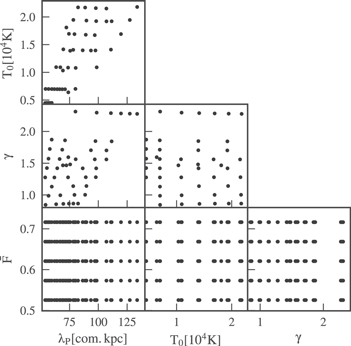
Figure 2. Subset of thermal models we used at z = 3.2. Each point in the  space corresponds to a different hydrodynamical simulation. Note the correlations between T0 (γ) and λP in the grid. For each simulation we rescaled the optical depths to obtain outputs with different mean transmitted fluxes
  .
.
Download figure:
Standard image High-resolution imageIn principle reionization is an inhomogeneous process (D'Aloisio et al. 2015; Davies & Furlanetto 2016), but we only use a homogeneous model to describe photoionizations. While generally UVB and thermal fluctuations could be influencing the power spectrum and therefore our conclusions on thermal evolution especially at z > 4 (see e.g., Cen et al. 2009), recent analyses (Onorbe et al. 2018, also earlier studies by McDonald et al. 2005 and Croft 2004 obtained similar results but with a focus on lower redshifts) have found that those mostly change the power spectrum on larger scales than used for this work (at least for  reionization), but does not strongly change the power on small scales, which provides most of the sensitivity to the thermal state of the IGM. Note again that we are not using the largest scale modes, which strongly reduces our sensitivity to inhomogeneities, further justifying our use of a homogeneous UVB.
We computed skewers of optical depth  by convolving each pixel along one-dimension in the simulation box with the corresponding Voigt profile for the temperature T,
  and Doppler shifts due to v for each simulation snapshot. As is common in Lyα forest studies (see, e.g., Bolton et al. 2010; Boera et al. 2014), the obtained values of τ were then rescaled to match different mean transmission values
  to compensate for our lack of knowledge of the UVB amplitude. Generally this rescaling will affect the shape and large-scale amplitude of the power spectrum. Lukić et al. (2015) investigated this issue (see their Figure 23) and found that rescaling τ by a factor of ∼0.5 results in ∼5% changes in the Lyα forest power spectrum, especially at low redshifts. While rescaling τ could be slightly biasing our results, we emphasize that the rescalings we perform in this work are typically smaller
  , and hence this effect should be subdominant compared to, e.g., box size effects and cosmic variance (see Section 6).
For each redshift and each parameter combination  we generated 50,000 randomly selected skewers—the same ones for each parameter combination—which serves as the starting point of our analysis.
4. Measuring the Thermal State of the IGM
In this section, we describe how we perform inference on our data using the THERMAL grid. This involves generating a forward model of the data, creating an emulator—a fast method to interpolate from a sparse grid of simulation to any point in the multi-d parameter space, and finally performing the actual inference via Bayesian methods.
4.1. Forward Modeling
To compare to existing measurements, which did not apply masking of spectral regions, but instead treated metal contamination statistically by comparing to lower redshift data where most metals are outside the Lyα forest, we compute the power spectrum based on ∼50,000 noiseless, high-resolution skewers from our simulation. We will refer to this as the "perfect model."
However, to account for the window function introduced on the power spectrum by masking parts of the data fully, when comparing to our measurement from Paper I, we compute the power spectrum based on the skewers for each combination of parameters applying the full forward modeling technique described in Paper I to our hydrodynamical simulations. Henceforth we will call this the "forward model." This technique consists of several steps of post-processing the hydrodynamical simulation outputs followed by a power spectrum computation in the same way as for the data. To forward model an individual quasar spectrum we first merge randomly selected skewers (without repetition) to cover the same path length as the data, then convolve the spectra with a Gaussian smoothing kernel reducing the resolution of the models to match that of the data, rebin the models onto the pixels of the observed spectra, and add noise drawn from a Gaussian distribution for each individual pixel with a standard deviation equal to the 1σ uncertainty of the corresponding quasar spectral pixel reported by the data reduction pipelines. Finally and most importantly, we mask the forward modeled spectrum in exactly the same way as the data to account for the windowing effects resulting from gaps in the data and our metal masking procedure. We then compute the power spectrum by utilizing ∼50,000 skewers from our simulation (see Paper I for a more detailed description of the individual steps). Note that while the full forward modeling of noise and resolution might not be completely necessary as they have been corrected in the measurement (and are corrected in the same way inside the forward modeling procedure as well), there might be subtle effects on the masking correction. We therefore want to make the model spectra as similar to the data as possible. Note that this does not change our model precision, which is dominated by data set size rather than noise or resolution.
4.2. Emulation of the Power Spectrum
To perform a fit to the data and infer the thermal state at a particular redshift we need to be able to compute power spectra on a continuous range of parameters. Therefore, we need to interpolate between the discrete and sparse outputs of the THERMAL grid. To perform this task we follow the emulation approach of Heitmann et al. (2006) and Habib et al. (2007). For details, we refer the reader to their papers (and references therein) as well as Paper I; in the following we summarize the main steps of the approach. First, we decompose the simulated logarithmic power spectra onto a principal component analysis (PCA) basis. We save the PCA vectors as well as the coefficients  at each thermal model location
  . We then use a Gaussian process (GP) to interpolate the coefficients
  onto any arbitrary location in parameter space
  . Taking the dot product of the PCA vectors with these interpolated coefficients then gives the power spectrum evaluated at any parameter location.
We thus calculate a GP for each principal component coefficient (using George, see Ambikasaran et al. 2016) using a squared exponential kernel plus an additional white noise contribution
for parameter values  , a chosen distance metric Cl (which is defined by a smoothing length l for each parameter, i.e., its diagonal) and a noise contribution σn (for an in-depth introduction to GP techniques, see Rasmussen & Williams 2005).
As the hydrodynamical grid consists of far less models (∼50)11 than the previous DM-based grid (∼500) used in Paper I, we must be more careful about the interpolation errors resulting from our emulation procedure. Instead of just using a kernel with a fixed hand-tuned smoothing length, which was our approach in Paper I, we additionally optimized our kernel parameters by maximizing GP-likelihood using the scipy.optimize (Jones et al. 2001) package and the so-called L-BFGS-B (Zhu et al. 1997) method.12 We then performed the analysis using the optimal smoothing lengths l and noise σn for the kernel for each GP emulator.
We estimate the emulation uncertainties using a cross-validation scheme to propagate interpolation errors. To do this we generate the emulator, but leave one simulation out of the training set.13
We denote emulators with a model (defined by parameters  ) left out as
  . We then compare the actual models (with power Pmodel) for this simulation to the emulator (with power
  ) at the parameters
  of this model:

We show the accuracy of the emulation in Figure 3. This shows quantiles of the deviations  from the true underlying model inside our cross-validation sample. We see that for most models in our parameter space the emulator works to better than 1%. However, emulation uncertainty can increase to the 5% level (with a preference for underestimation at
  ) for some models. As the uncertainty in our power spectrum measurements is ∼2% (for the 68% quantile) on large scales (k ≲ 0.01
  ) and ≳5% on smaller scales, measurement errors are much larger than these interpolation errors. Nevertheless, we opted to add the covariance matrix for the interpolation process to our likelihood. This covariance matrix can be obtained by performing:

with the average performed over all possible combinations of model parameters inside our grid for each redshift bin.

Figure 3. Cross-validation results for our emulation procedure at z = 2.8. Colored bands show the relative difference between emulated and true power for different cuts of the full cross-validation set. The median is shown as a black curve. Other redshifts give similar results especially for the 68% region. See the main text for more details.
Download figure:
Standard image High-resolution imageDue to the variety of thermal histories in the THERMAL suite some simulations can have extremely close values of their thermal parameters at some specific redshifts. In order to avoid possible problems in the emulator due to this issue we removed models from the THERMAL grid that did not satisfy a distance threshold14 and are left with 45–65 models per redshift.
4.3. Inference
We perform a Bayesian MCMC analysis on the power spectrum data at each individual redshift using the emcee package (Foreman-Mackey et al. 2013) based on the affine invariant sampling technique (Goodman & Weare 2010) and assuming the multivariate Gaussian likelihood:
with Cemu being the covariance of the interpolation procedure and Cdata being the covariance of an individual measurement. For these covariances we use published values if available. For our own data set from Paper I as well as the Viel et al. (2013) data set, we used the published uncertainties (i.e., the diagonal covariance elements) and combined them with the correlation matrix of the model closest in parameter space to obtain an estimate of the covariance, i.e., we perform nearest neighbor interpolation between covariance matrices obtained at every point (see Paper I for details on this approach).
4.4. Parameters and Priors
Our modeling so far depends on four parameters, T0 and γ describing the thermal state, λP for the pressure smoothing depending on the full thermal history, and  for the mean transmission that corresponds to a given UVB amplitude. There is, however, one additional parameter that we input in our models for each data set15
to generate the observed correlation between
for the mean transmission that corresponds to a given UVB amplitude. There is, however, one additional parameter that we input in our models for each data set15
to generate the observed correlation between  and Lyα (see McDonald et al. 2006; Palanque-Delabrouille et al. 2013). Finally, because of significant uncertainties in the resolution of the XQ-100 data (see the detailed discussion in Appendix B of Paper I), we also marginalize over the resolution of the XQ-100 measurement whenever we use this data, giving us another parameter. Therefore, we have a total of five (in the case of high-resolution data only) to eight (in the case of fitting 3 data sets of which one comes from XQ-100) parameters. We assume flat priors on
  . We now go into further detail about the modeling and assumptions for the other parameters.
We add  correlations to the model analytically by multiplying the model power spectrum with an oscillating signal as correlations inside a spectrum correspond to oscillations of the corresponding power spectrum:

with  being a free nuisance parameter for the strength of the correlation. In previous works this was typically expressed as
  with
with  being a redshift independent quantity that was fit using the entire data set. We adopt this same parametrization but opt to fit for a unique value of
  at each redshift and for each data set because of the different metal treatment in the data sets and as we do not perform a joint fit of different redshifts here. We assume a flat prior on each
  and demand correlations to be positive.
We modeled the resolution of the XSHOOTER spectrograph Rnew by multiplying the measured XQ-100 power spectrum with the resolution dependent part of the window function:

using the resolutions quoted in Iršič et al. (2017a) and dividing by  . Note that the resolution of the instrument depends on two different factors: the resolution for a fully illuminated slit (or "slit resolution") and the seeing, which gives rise to higher spectral resolution if smaller than the slit size. We assume two limits for the resolving power of the XQ-100 data set. The lower limit assumes the slit resolutions quoted in the XQ-100 data release paper (López et al. 2016) as well as a fully illuminated slit (leading to
  for the UVB arm of the instrument,
  for the VIS arm16
). The upper limit assumes a seeing of 0
for the VIS arm16
). The upper limit assumes a seeing of 0 65 (smaller than the slit) and higher values for the slit resolution17
(leading to RUVB = 8230 and RVIS = 12184). We assume a flat prior between these two limits. As z = 3.6 is using both spectral arms we use the lowest and highest of the four resolution values above as the limits here. Note that this choice of priors on spectroscopic resolution is an extremely conservative choice that will significantly weaken the constraints that can be obtained from this XQ-100 data set. This is most acute in the UVB arm because of its intrinsically lower resolution. A more careful analysis of the XQ-100 resolution would allow us to adopt a far stronger prior on these values, which would increase the precision of constraints deduced from power spectra measured from such moderate resolution spectra.
65 (smaller than the slit) and higher values for the slit resolution17
(leading to RUVB = 8230 and RVIS = 12184). We assume a flat prior between these two limits. As z = 3.6 is using both spectral arms we use the lowest and highest of the four resolution values above as the limits here. Note that this choice of priors on spectroscopic resolution is an extremely conservative choice that will significantly weaken the constraints that can be obtained from this XQ-100 data set. This is most acute in the UVB arm because of its intrinsically lower resolution. A more careful analysis of the XQ-100 resolution would allow us to adopt a far stronger prior on these values, which would increase the precision of constraints deduced from power spectra measured from such moderate resolution spectra.
Note that most previous measurements (exceptions to this are, e.g., Lidz et al. 2010; Iršič et al. 2017b) of the IGM's thermal state did not attempt to marginalize over the uncertainty in the mean flux estimate. Instead, typically simulations that match the mean flux of the data assuming perfect knowledge of this quantity are used (e.g., in Voigt profile fitting or curvature analyses). For  we used both a flat prior (corresponding to performing a joint measurement of
  and the thermal state) and a Gaussian-shaped prior. For the Gaussian prior we assumed a mean based on the fit by Oñorbe et al. (2017a) to a compilation of recent measurements (Fan et al. 2006; Kirkman et al. 2007; Faucher-Giguère et al. 2008b; Becker et al. 2013) and a standard deviation based on the uncertainties for the most recent measurements at z ≤ 4.0: Becker et al. (2013) for
  , Faucher-Giguère et al. (2008a) for z = 2.0, and Kirkman et al. (2005) for z = 1.8. For z ≥ 4.2 we use
  , which is loosely based on the discrepancy between Fan et al. (2006) for z ≥ 4.6 and the measurements by Becker et al. (2011) in the range 4.1 ≤ z ≤ 4.7 (see also Bosman et al. 2018; Eilers et al. 2018, for more recent mean flux measurements that are discrepant by a similar amount for 5.0 ≤ z ≤ 5.4).
To avoid extrapolating from our model grid we additionally require that all thermal parameters lie inside the convex hull of our model grid (see Figure 2), i.e., the smallest convex shape, including all THERMAL grid points. The convex hull is evaluated numerically by triangulating the model grid (using scipy.spatial.Delaunay) and for each MCMC sample we test whether it is inside the triangulation when evaluating the prior. Otherwise the prior is set to zero. To see the effective prior resulting from only using this non-rectangular region where we have models, we performed an MCMC run assuming a completely uninformative data set, i.e., using only the priors in our fit and a constant likelihood. The results of this procedure are shown in Figure 4 for z = 2.8. In some contours, e.g., T0 and λP, we can see that the parameters are highly correlated already since our grid is non-rectangular. We argue, however, that these correlations are physically motivated as models perpendicular to these correlations are hard to produce (see Section 3) and that this behavior actually constitutes prior information for our analysis.
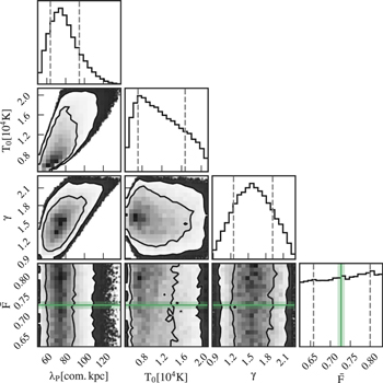
Figure 4. Corner plot showing the prior PDF for the thermal parameters and  given our model grid and excluding parameter values outside its convex hull. This was obtained by sampling our prior with an MCMC, assuming a flat likelihood. Note that the degeneracies in our model grid lead to non-flat marginalized distributions. The diagonal shows the 1d-PDF (marginalized over all other parameters) for each parameter with dashed vertical lines at the 16% and 84% quantiles. The scatter plots below show the 2d-PDFs for each combination of two parameters (also marginalized over all others) with contours showing the region containing the 68% and 95% highest densities. Note that due to the restrictions of our grid there is a strong correlation especially between T0 and λP. The additional preference toward low T0 or λP is due to our choice of flat priors in the log of these parameters. The green band shows the 1σ interval in
  we use for the Gaussian prior.
Download figure:
Standard image High-resolution image5. Thermal Evolution of the IGM
5.1. Measurements and Degeneracies
We performed fits of the parameters governing the thermal state using combinations of all data sets discussed in Section 2 in 16 individual redshift bins with 1.8 < z < 5.4, where we used a bin size Δz = 0.2 for z ≤ 4.2 and Δz = 0.4 for z ≥ 4.6.
The power spectra of each data set are summarized and compared to models based on our posterior MCMC chains in Figure 5. Note that for visualization purposes we only compare window function,  correlation, and resolution corrected data to the perfect model. The window function due to masking was taken out of the UVES/HIRES data by multiplying measurement points with the median
  for our MCMC chain and propagating its uncertainties using Gaussian error propagation for each individual mode (see Paper I for a more detailed description of this process).18
Analogously, we rescaled the XQ-100 power to use the "best-fit" resolution correction, i.e., we renormalize with
for our MCMC chain and propagating its uncertainties using Gaussian error propagation for each individual mode (see Paper I for a more detailed description of this process).18
Analogously, we rescaled the XQ-100 power to use the "best-fit" resolution correction, i.e., we renormalize with  (see Equation (8)) from the posterior and removed
  correlations from the data applying Equation (7). We can see that satisfactory fits have been achieved at all redshifts.
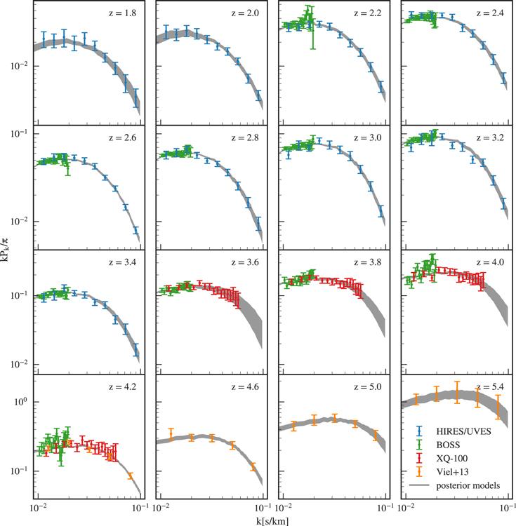
Figure 5. Redshift evolution of the power spectrum with colors showing different data sets. Data by Iršič et al. (2017a) were corrected to the median of the marginalized posterior resolution, Walther et al. (2018) points have been corrected for the masking window function. All data have been corrected for  correlations. Bands show 68% confidence regions for our emulator with parameters randomly drawn from the posterior distribution.
Download figure:
Standard image High-resolution imageIn Figure 6, we further illustrate the posterior distribution is inferred via our MCMC at z = 2.8 with a so-called "corner plot." We can see that the data strongly constrains all parameters (e.g., compare to Figure 4 or the blue curves in the 1d histograms, for which the likelihood is assumed to be completely uninformative). The most important feature we see is that there are strong degeneracies between some parameters, e.g., the diagonal contours between permutations of T0, γ, and  . Note that the strong correlation between T0 and γ is well understood and results from the IGM not probing the mean density, but instead mild overdensities at these redshifts (see, e.g., Lidz et al. 2010; Becker et al. 2011). We also infer a low mean transmitted flux
  compared to the Becker et al. (2013) measurement of
  (green band). It is interesting to note that this low value however agrees well with the joint constraint on mean transmission evolution by Palanque-Delabrouille et al. (2015) obtained from the BOSS power spectrum yielding
  for
for  resulting in
  . Note that the data set used in this analysis overlaps with the one we used here, but the simulations and inference procedure are independent and our analysis has additional higher resolution data available. Independent of the BOSS data, we also obtain similarly low
  values when performing fits on the high-resolution data from Paper I alone.
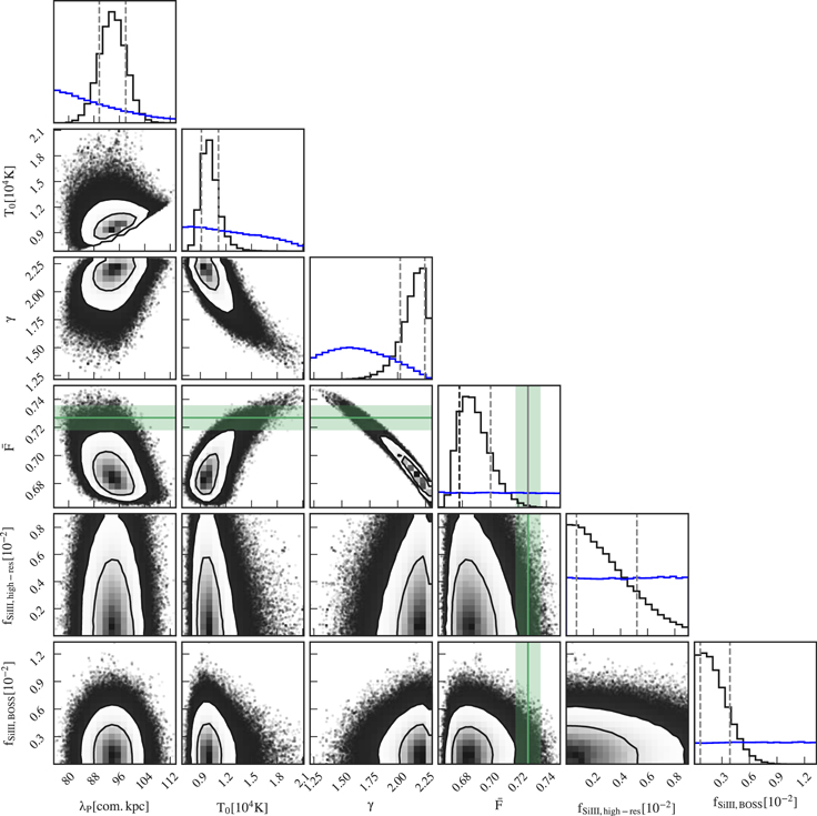
Figure 6. Corner plot showing 1d- and 2d-marginalized posterior distributions for all fitting parameters at z = 2.8, assuming a flat prior on  . Blue curves in the 1d histograms show 1d-marginalized distribution when ignoring the data and fitting the prior only (i.e., the result of the analysis performed for Figure 4). We can see that there are strong constraints on all parameters compared to the prior information. We also notice a strong correlation between permutations of γ, T0, and
  . Note that the posterior in
  is significantly below the observed value of the Becker et al. (2013) mean flux measurement (shown as a green line with a band for the 1σ region), which is, combined with the strong anticorrelation between γ and
  , leading to higher values of γ than typically assumed.
Download figure:
Standard image High-resolution imageAdditionally, the posterior distribution for γ shows a clear preference for values γ ≈ 2.1, far above the expected value of ∼1.6 for IGM gas in photoionization equilibrium long after reionization events (Hui & Gnedin 1997; McQuinn & Upton Sanderbeck 2016) Note again that there is a strong anticorrelation between γ and  , so while our analysis prefers a high value of γ and a low value of
  , this is a movement along the degeneracy direction. We will further discuss this issue in Section 5.2.
The redshift evolution of individual parameters, determined from the 1d-marginalized posteriors, is illustrated in Figure 7. For 3.0 ≤ z ≤ 3.4 we also performed fits including the XQ-100 data, and fully marginalized over our lack of knowledge of the exact spectroscopic resolution (see discussion in Section 4.4). As including this data set did not significantly change our results, we decided to leave those points off the plot for clarity. Numerical values for the marginalized parameters are tabulated in Table 3 (see the

Figure 7. Points with error bars show the median and the region between the 16% and 84% quantiles of the three thermal parameters as well as the mean transmission of the IGM (marginalized over all model parameters of the fit) at different redshifts using our fiducial data set (squares) at each redshift. In the  panel we also show the evolution obtained by Becker et al. (2013; red band showing 1σ uncertainties) based on relative changes in Sloan Digital Sky Survey quasar transmissions as well as the Oñorbe et al. (2017a; dashed line) fit to these data and further data sets. Note the large discrepancies between our measurements and those results when assuming an uninformative prior on the mean flux. The white range shows the space populated by our models, i.e., we cannot expect to measure values inside the gray shade using our current emulator.
Download figure:
Standard image High-resolution imageThere are several noteworthy features in Figure 7. First, the disagreement that we saw at z = 2.8 between our inferred value of  and recent measurements is also present at all other redshifts z < 3 (green and blue data points compared to the pink-shaded region in the lower panel). At the same time γ reaches very high values in the same redshift range. Also, T0 drops strongly from z = 3.0 to lower redshifts, but due to the degeneracies between T0, γ, and
  , these measurements are all strongly correlated and this effect is therefore expected. Note that these trends—high γ, low
  , and low T0—persists if we fit the high-resolution data alone, as the BOSS data alone do not individually constrain all of these parameters due to the lack of high k-modes (resulting from limited spectral resolution).
Second, for z ≥ 3 we can see that γ shows little evolution and the mean transmitted flux  is consistent with the Oñorbe et al. (2017a) fit to recent measurements. We can also see that T0 increases from ≈5100 K at z = 5.0 to
  at z = 3.4. This rise could be explained by the onset of
  reionization, which we discuss in more detail in Section 5.5 where we compare our inferred parameter values to models of IGM thermal history that treat reionization heating.
In summary, we can see that the power spectrum analyzed here can in principle achieve high-precision constraints on IGM thermal parameters and the mean transmission, but the high values of γ ≃ 2 inferred at z < 3 and concomitant discrepancies between our inferred mean flux and the Becker et al. (2013) measurements might indicate systematics in our procedure. We consider this issue in detail in the next section.
5.2. Analyzing the Discrepancies in  and
and


In the previous section we found low values of  compared to Becker et al. (2013) and possibly unphysically high values of γ. While both parameters are degenerate and the degeneracy direction matches with our discrepancy this might point toward some problem within the analysis. To investigate this scenario we want to isolate the change in the power spectrum when moving along the degeneracy direction of our posterior distributions. Due to the dimensionality of the parameter space and correlations between different parameters this cannot be achieved by simple cuts along a parameter direction. Therefore, we designed the following procedure to generate model curves tracking the degeneracy direction for different values of γ (also see the illustration in Figure 8):
- 1.We take the posterior of our MCMC analysis (i.e., the Markov chain) and define bins such that the median of γ inside a bin is equal to a desired quantile of the marginalized γ distribution (which are chosen to be equivalent to ±1σ, ±2σ). These bins are shown as colored bars in the left panel of Figure 8.
- 2.For γ values in our chain within a given bin, we then compute the median of all other parameters. Because of the way we chose our γ bins, this yields the quantile of interest for γ, whereas the other parameters will track their corresponding degeneracy direction with respect to γ. This can be seen in the colored squares in the right panel of Figure 8.
- 3.For the set of parameters at each of the quantiles (e.g., the 84% quantile in γ and the median in all other parameters for the corresponding bin) we can then generate a model using our GP emulator.
The result of this procedure is shown in Figure 9 for the power spectrum at redshift z = 2.8, which is the highest redshift showing a high γ value. We compare models generated in this way to the measured power spectra shown as the blue and green points in the figure. Bands show the 68% confidence interval at each k for models generated using our emulator with random draws from the posterior distribution. Note that the forward model (due to both masking and forward modeling of noise and resolution) can generate slightly more converged model power spectra than the perfect model using the same parameters. The latter band is therefore actually a prediction for k ≳ 0.02  and its slightly larger extent is not surprising. Also note that due to the way we chose to produce curves with different thermal parameters and the dimensionality of the space the range spanned by the dashed curves is typically smaller than the colored bands. This is expected as the band shows the actual spread in the five/six (depending on the number of data sets used) dimensional parameter space, whereas the lines are based on a quantile for one of the parameters and values at the center of the distribution close to that quantile for all others, which will lead to a point inside the respective hypersurface, e.g., parameters of the purple/blue curve fall inside the five/six dimensional 68% surface, where the band corresponds to the actual surface).
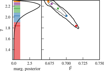
Figure 8. Illustration for our approach in selecting models along the posterior distribution (see the main text for details). Left: the marginalized posterior distribution of γ values from our chain with the bins that we used to generate models at the 68% and 95% confidence intervals shown as bars. The median chain value in each bin is shown as a colored line. Right: 68% and 95% contours for γ vs.  with the selected values of both parameters shown as squares.
Download figure:
Standard image High-resolution image
Figure 9. Topmost panel: the power spectrum (not corrected for masking) at z = 2.8 (other redshifts are shown in Figure 10, bands are showing regions in which 68% of models in the posterior fall) with curves showing models (drawn from the respective emulator) with different thermal parameters. Those are chosen such that the lines represent the 2.5%, 16%, 50%, 84%, and 97.5% quantiles of the posterior distribution in γ, while following degeneracies with the other parameters (see main text and Figure 8 for the details). Values of the most relevant parameters are printed inside the figure (with  ). Both data sets have been offset by a factor of 2 for clarity. Bottom panels: the fractional deviation between data in the topmost panel and the model at median γ (green curve) for each data set.
Download figure:
Standard image High-resolution imageWe can see that all five models shown basically lead to the same power except for the highest k-values measured k ≥ 0.07 (smallest scales). At those scales a higher γ and lower  indeed seem to provide a better fit to the data, whereas at larger scales (smaller k) the model does not seem to be strongly affected by the parameters when moving along the degeneracy.
However, for other redshift bins (see Figure 10) the sensitivity of the power spectrum toward changes in γ for a region around the median value shifts to different scales. For example, at z ≤ 2.0 the most dominant effect seems to be on large scales, but note that we do not have the high-precision BOSS measurement and therefore both the range in allowed power spectra and the range of parameters in the 2σ region of γ are larger. All other redshifts seem to suggest a highest sensitivity to γ at scales k ∼ 0.05  , different from both the lowest redshifts and z = 2.8. While we note that differences between models of different γ along the degeneracy direction are typically small compared to our measurement errors for an individual k-bin, it is clear that the data of all bins combined has the precision to distinguish between these models, and that our inference is producing sensible fits. One might argue that the fact that the k-modes that are driving the fits to high γ and low
  change for different redshift bins is a source of concern, but we caution that the degeneracies in this multi-dimensional parameter space are complex and not always easy to visualize. We are confident that these results are not spurious, since this high γ, low
  combination persists consistently across all redshift bins with z ≤ 2.8, and both measurements and our inference of different redshift bins are completely independent. We will return to this issue of discrepant γ and
  values in Section 6 when we discuss possible systematic errors in our hydrodynamical simulations.
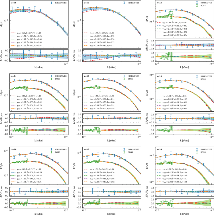
Figure 10. Same as Figure 9, but also for all redshifts  . We can see that while most redshift bins show the strongest scatter in the power at
  when moving along the degeneracy direction. However, for z = 1.8, 2.0 the behavior seems to be significantly different most likely due to the lacking precision on small k due to the lack of the BOSS measurement at these redshifts.
Download figure:
Standard image High-resolution image5.3. Measuring Thermal Evolution in the IGM Using a Gaussian Prior on the Mean Transmission
Given that independent precise constraints on the mean transmission exist we now consider the effect of applying a Gaussian prior on the mean transmission based on these measurements (see discussion in Section 4.4 for details). Henceforth we will refer to these fits as the "strong prior" results, and we will designate them as our fiducial measurements (as opposed to the joint fits for thermal parameters and  described in previous sections). Note that most previous analyses of the IGM thermal properties have simply assumed perfect knowledge of the mean transmission (see Lidz et al. 2010; Iršič et al. 2017b for exceptions), such that this "strong prior" approach is more consistent with previous efforts.
We present the redshift evolution of posterior parameter degeneracies assuming the strong prior in Figure 11. Each panel in these figures shows the 2d-marginalized 68% and 95% confidence regions of T0 versus γ. While γ and T0 are strongly anticorrelated at low redshifts z ≤ 3.4, i.e., the contours are close to diagonal, this correlation gets weaker at higher redshifts (especially at z ≥ 4.2), i.e., contours become aligned with the axes due to lower overdensities probed by the power spectrum. Likewise, the γ versus  confidence regions are shown in Figure 12. Note that these properties are correlated independent of redshift, in stark contrast to the thermal parameter degeneracy, while still changing shape and direction due to the different precision of the measurements. Therefore, a change of prior for the mean transmission measurements propagates into γ at high redshifts (z ≥ 4.2), but does not affect T0 significantly. At lower redshifts (especially for z ≤ 3.4), however, γ is strongly correlated with both T0 and
  , so a change in priors for any of the three quantities always affects the results on the other two quantities as well. Consequently, the change in our mean flux prior affects lower redshifts (especially z < 3) more strongly than higher ones.
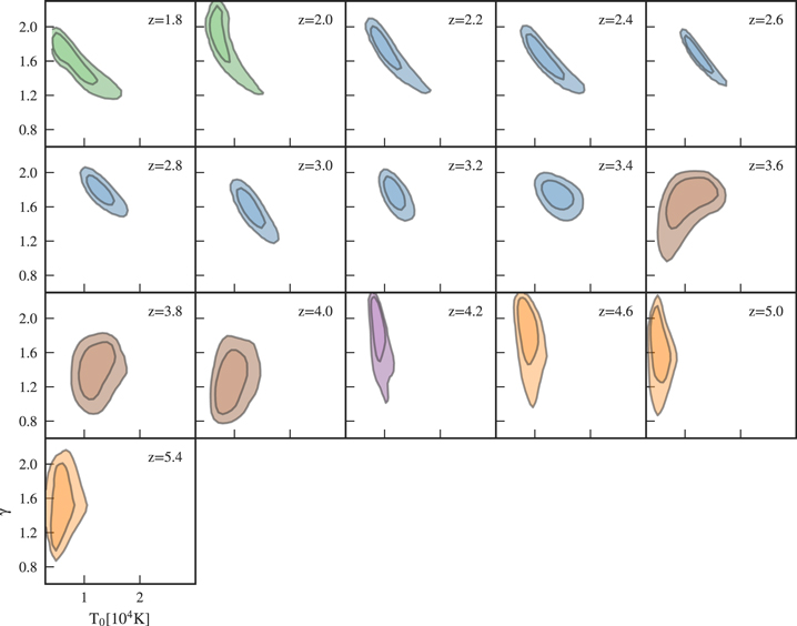
Figure 11. Evolution of the T0 vs. γ contours with redshift assuming the strong prior on  for different combinations of data sets (different colors matched to Figure 7, contours showing the 68% and 95% confidence regions. When high-resolution data is used we can see that strong constraints perpendicular to a degeneracy direction can be obtained. We can also see that this degeneracy direction rotates as the Lyα forest probes higher and higher densities.
Download figure:
Standard image High-resolution image
Figure 12. Same as Figure 11 but with  vs. γ contours. This shows that independent of redshift, γ and
  are strongly anticorrelated.
Download figure:
Standard image High-resolution imageWe show the fully marginalized posterior constraints on thermal parameters as a function of redshift in Figure 13 (for tabulated values, see Table 4 with further details in the
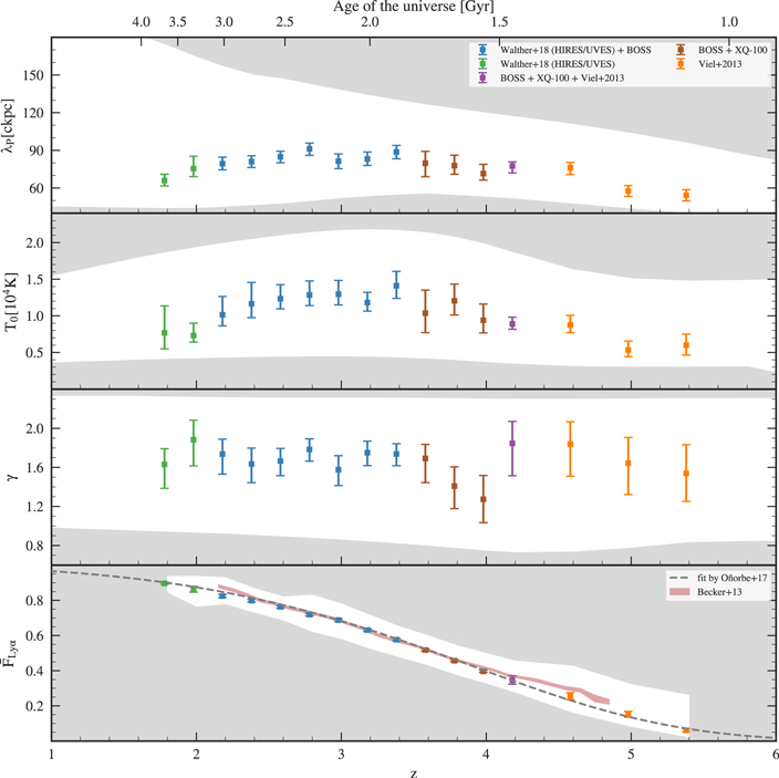
Figure 13. The fiducial measurements from Figure 7, but assuming a Gaussian prior on the mean transmission complying with the fit of the Oñorbe et al. (2017b) measurement within error bars given by observations (Kirkman et al. 2005; Faucher-Giguère et al. 2008a; Becker et al. 2013). We can see that now the obtained γ values at low redshifts are far lower (and compatible with the expected value of 1.6 long after reionization) due to the additional mean transmission constraint. The high values of γ at high redshifts obtained here are likely due to the discrepancy of the mean of our chosen prior (dashed curve) with the Becker et al. (2013; red band) analysis for the mean transmission. Due to the far lower overdensities probed at high redshifts compared to low redshifts, these high values of γ do not change the results on T0 strongly, as degeneracies are largely broken (see also the evolution of the T0–γ and γ– contours, which can be found in Figures 11 and 12 ).
Download figure:
Standard image High-resolution image
Figure 14. Comparison of our results on the thermal state dependent on redshift between both priors (different colors). We can see that the flat prior leads to far higher values of γ causing lower values of T0 due to correlations between to lower values of T0.
Download figure:
Standard image High-resolution imageHowever, this is the first thermal evolution measurement performed over the whole epoch of  reionization and beyond based on the power spectrum. Using the strong mean flux prior we also obtained reasonable results, including physically possible measurements of γ, a rise in temperature for z ≳ 3 as time progresses (or redshift decreases), and the first measurement of the IGM cooling down thereafter. In the next sections we compare our strong prior results to recent thermal parameter measurements from different methods as well as models of IGM thermal evolution.
5.4. Comparison to Previous Measurements
A comparison of our results to recent measurements of thermal parameters is shown in Figure 15. We discuss the various data sets involved and elaborate on the comparison to our new measurement below.
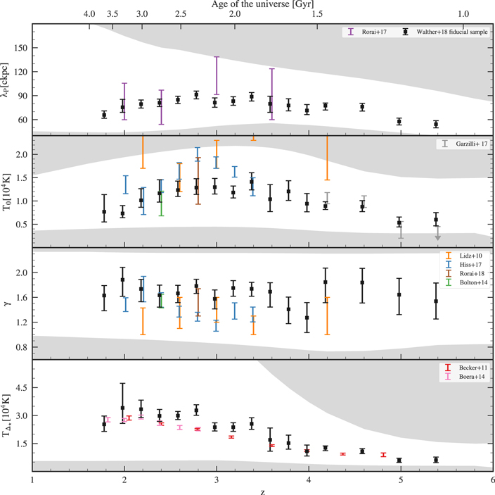
Figure 15. Fiducial data from Figure 13 (black points) assuming the strong Gaussian prior on  . In addition to the previous plots we show the thermal parameters as well as T(Δ⋆) at the optimal overdensities Δ⋆ for curvature measurements as given by Becker et al. (2011). We compare to measurements of thermal evolution in the IGM based on different statistics: curvature (red, pink), line fitting (green, blue, brown), wavelets (orange), phase angles (purple), and power spectrum (gray). We can see overall good agreement with previous data sets (except for wavelets), albeit a significantly higher T(Δ⋆) than in the curvature measurements is obtained at some redshifts. All measurement errors shown are 1σ or 68% intervals, and for measurements that only quote 2σ error bars, we divided those by a factor of 2.
Download figure:
Standard image High-resolution imageThe phase angle PDF of quasar pairs (Rorai et al. 2013) measures the smoothness of the 3d distribution of IGM gas and therefore directly constrains the pressure smoothing scale λP independent of the instantaneous thermal state of the IGM (i.e., T0 and γ). Rorai et al. (2017b) measured λP from a sample of quasar pairs in four redshift bins between  . Figure 15 shows that our inferred values of λP are fully consistent with the Rorai et al. (2017b) measurement. We also see a smaller uncertainty in our power-spectrum-based measurement. Part of the explanation for these small error bars lies in how our model grid, and therefore our prior probability, is set up. As discussed in Section 4.4, the degeneracy between T0 and λP within our simulated models combined with our approach of not extrapolating to regions outside our model grid result in a positive correlation in the prior probability between these parameters. However, the power spectrum cutoff is sensitive to a degenerate combination of both λP and thermal broadening (Peeples et al. 2010; Rorai et al. 2013), leading to an anticorrelation in the likelihood. So the correlations inside our prior (Figure 4) and the degeneracy direction of the likelihood due to the aforementioned effect are nearly perpendicular, and as the posterior distribution is the product of these two, the resulting constraints appear very tight. However, we argue that it is hard to generate physical models without imprinting the correlation between thermal state and λP that depends on the integrated thermal history of the IGM. While the uncertainties in λP might still be somewhat underestimated, we note that our prior grid degeneracy has a strong physical motivation (see also Section 4.4).
The orange points in Figure 15 show the T0 and γ measurements from Lidz et al. (2010), who decomposed the Lyα forest of the Dall'Aglio et al. (2008) data set into wavelets and analyze the PDF of their squared amplitudes to derive constraints on the thermal state of the IGM. We note that this data is a subset of that used to compute the power spectrum in Paper I and analyzed here. Note that their γ constraint is often limited to the boundaries of their fits.19 While the wavelet analysis results at z = 2.6 are consistent with our measurement, we disfavor the z = 2.2, z = 3.0, z = 4 and especially z = 3.4 wavelet results, which seem to indicate a far hotter IGM than our measurement. The origin of this discrepancy is unclear, but it has also been noted before by Becker et al. (2011).
Another method for obtaining constraints on the thermal state of the IGM is by decomposing the Lyα forest into individual absorption lines, assuming that a cutoff in the distribution of column densities  versus Doppler parameter b exists and can be attributed to lines that are only thermally broadened (see, e.g., Schaye et al. 2000; Rudie et al. 2012; Bolton et al. 2014; Hiss et al. 2018; Rorai et al. 2018). Especially the new Hiss et al. (2018; which is based on the same data set as Paper I and is using a subset of the same simulation grid) thermal evolution result seems to hint toward a period of heating until z ∼ 2.8 that could be attributed to
  reionization.
For both T0 and γ we see broad agreement between our measurements and the line-fitting results at most redshifts. Of particular interest are z = 2.4 and z = 2.8, where several line-fitting measurements exist. At z = 2.4 we do reproduce the result from Hiss et al. (2018; blue points) as well as Bolton et al. (2014; green) in both T0 and γ. At z = 2.8 we agree with the Rorai et al. (2018; brown point), but obtain higher precision. However, agreement with Hiss et al. (2018) at this redshift seems to be poor as they measure both higher T0 and lower γ (which is along the degeneracy direction for line-fitting analyses as well as the power spectrum). Part of this discrepancy might come from systematics in the Voigt profile analysis, depending on the cutoff fitting algorithm chosen, as Hiss et al. (2018; see Appendix B) find either a multimodal posterior probability distribution for T0, γ with a similar 68% confidence interval as Rorai et al. (2018), or a unimodal distribution with the values shown here depending on the cutoff fitting algorithm used. Whether this multimodal behavior results from systematics in the measurement procedure or is a real physical effect from, e.g., a real multimodal IGM TDR is not yet clear, but we do not see such behavior in our power spectrum analysis. For the other overlapping redshifts (except z = 2.2 and z = 2.4, which match very well) we generally measure a lower T0 and higher γ compared to Hiss et al. (2018).
The most precise measurements of temperature in the IGM so far are based on the mean curvature in the Lyα forest  (Becker et al. 2011; Boera et al. 2014). These measurements constrain T(Δ⋆) at an optimal overdensity Δ⋆ at which a one-to-one relation between the mean curvature
  of the Lyα forest and T(Δ⋆) exists independent of the slope γ of the TDR (note again Figure 11, which shows the corresponding degeneracy for the power spectrum). However this method is not able to measure γ or T0 independently. To compare to curvature-based measurements, we compute
  (using the values for
  given by Becker et al. 2011) for each sample in our MCMC chain and evaluate the 68% confidence interval. This approach allows us to directly compare to what the curvature results measure.
The agreement with the curvature analysis seems to be generally good for the largest part of the overlapping redshift range, but we seem to measure overall slightly higher temperatures. There are some redshifts  where our analysis gives significantly higher temperatures than implied by the curvature measurements. Note in particular that at z = 2.8, where we see the strongest discrepancy between our results and the curvature measurements, multiple measurements of the thermal state have been performed via several different methods, and these results do not fully agree with each other. We argue that the overall agreement is still good given the significantly different data sets, statistical approaches, and models used for both types of analysis. For example, the difference in measured thermal state might potentially arise due to the different sensitivity of both statistics to metal contamination. While the power spectrum is only weakly affected by residual metal lines on the very smallest scales we cover here (see the comparison in Walther et al. 2018), the averaged squared curvature is basically measuring
  (see Appendix D in Puchwein et al. 2015) and thus enhances the weight of residual small-scale contamination in the Lyα forest. At the same time small-scale contaminants, like, e.g., leftover metal lines, would decrease the obtained IGM temperatures as there is now too much small-scale power, thus leading to a colder IGM in curvature than in power spectrum analyses. Additionally, these measurements did not marginalize over the mean flux in the simulations, thereby, e.g., potentially underestimate their errors.
Finally, we also show the Garzilli et al. (2017) measurement of T0 at  based on the same as the Viel et al. (2013) data set we use here (gray points, the limit is at the 1σ level), but using a different analysis pipeline and including a WDM particle mass as an additional free parameter. We can see that for
  the agreement is good, but for z = 5.4 we seem to get slightly higher values of T0 than their 1σ upper limit. Part of that difference can be attributed to the additional freedom in their model.
Overall, we conclude that the agreement between our data and previous results is reasonably good. Our measurement is a strong advancement with regard to previous analyses, especially due to the large range of uniformly covered redshifts and due to jointly constraining T0 and γ over this full range.
5.5. Comparing to Thermal Evolution Models for Different He ii Reionization Scenarios
In the previous sections we performed a self-consistent measurement of thermal evolution in the IGM from z = 5.4 to z = 1.8, corresponding to 3 Gyr of cosmic history. In this section, we compare to simulations to thermal evolution due to  reionization, as this is expected to be the dominant process setting the thermal state of the IGM at this epoch.
In Figure 16, we show comparisons between our thermal evolution measurement and models based on different approaches. The solid curves show the "explicit reionization" simulations from our model grid for which hydrogen reionizes (to a level  , note that for our models this point is typically reached with a delay of
  compared to the corresponding
  20
) at
20
) at  in agreement with the Planck Collaboration et al. (2016a; and also Planck Collaboration et al. 2018) constraints, but for which the parameters governing
  reionization are varied (see Table 2). The red dashed-dotted curve is showing an extreme version of these models for which
  was never reionized.21
The measured temperature at mean density is significantly higher (by ≳3σ for each of the seven individual redshift bins with 2.2 ≤ z ≤ 3.4) than this "no
was never reionized.21
The measured temperature at mean density is significantly higher (by ≳3σ for each of the seven individual redshift bins with 2.2 ≤ z ≤ 3.4) than this "no  " scenario for z ≤ 4.6 suggestive of a period of
  reionization taking place.
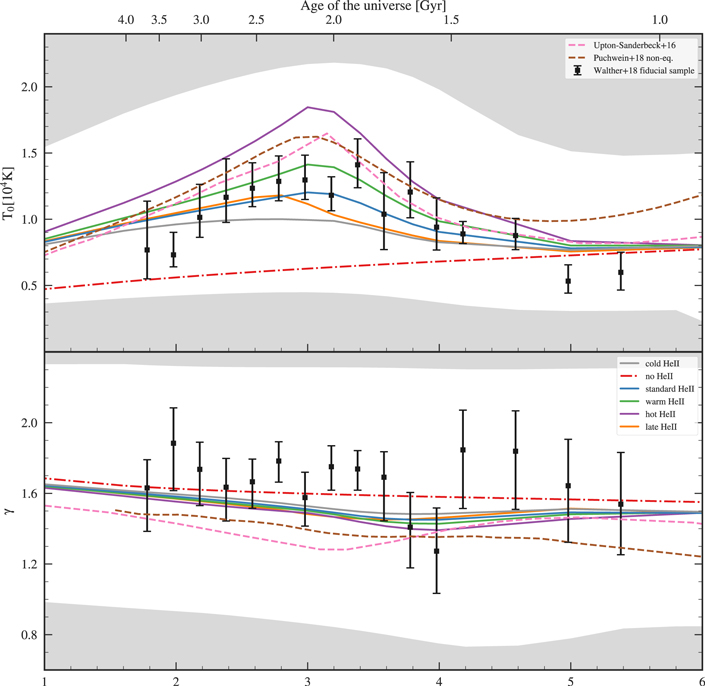
Figure 16. Fiducial data assuming the strong Gaussian prior from Figure 13 (black points) compared to thermal evolution models assuming different redshifts of  reionization and heat inputs during this process (solid curves) and without any
  reionization (dotted-dashed red curve). The model parameters are given in Table 2. We also show comparisons to the Upton Sanderbeck et al. (2016; dashed pink) thermal evolution model and a run using the Puchwein et al. (2018) non-eq. heating rates in a Nyx simulation (dashed brown). We can clearly see that the data shows a hotter IGM than created in the model without
  reionization. Instead, the overall evolution of thermal parameters seems to agree well with the standard to warm
  reionization scenarios in both T0 and γ. Finally, the temperatures found at the two highest redshift bins are colder than any model.
Download figure:
Standard image High-resolution imageTable 2 .
Thermal Evolution Models Used in Comparisons to Existing Measurements: Parameters are the Reionization Redshifts and the Total Heat Input during Reionization for  and
and  , see Oñorbe et al. (2017a) for Details
| Model Name |

|

|
![${\rm{\Delta }}{T}_{{\rm{H}}{\rm{I}}}[{\rm{K}}]$](https://content.cld.iop.org/journals/0004-637X/872/1/13/revision1/apjaafad1ieqn163.gif)
|
![${\rm{\Delta }}{T}_{\mathrm{He}{\rm{II}}}[{\rm{K}}]$](https://content.cld.iop.org/journals/0004-637X/872/1/13/revision1/apjaafad1ieqn164.gif)
|
|---|---|---|---|---|
No 
|
7.3 | ⋯ | 20000 | ⋯ |
Cold 
|
6.55 | 3.0 | 20000 | 10000 |
Standard 
|
6.55 | 3.0 | 20000 | 15000 |
Warm 
|
6.55 | 3.0 | 20000 | 20000 |
Hot 
|
6.55 | 3.0 | 20000 | 30000 |
Late 
|
6.55 | 2.8 | 20000 | 15000 |
Download table as: ASCIITypeset image
Table 3.
Fiducial Evolution of Thermal Parameters Assuming a Flat Prior on 
| z | λP | T0 | γ |

|

|

|

|
|---|---|---|---|---|---|---|---|
| (kpc) | ( ) ) |
( ) ) |
( ) ) |
||||
| 1.8 |

|

|

|

|

|

|
1.705 |
| 2.0 |

|

|

|

|

|

|
1.437 |
| 2.2 |

|

|

|

|

|

|
1.638 |
| 2.4 |

|

|

|

|

|

|
1.841 |
| 2.6 |

|

|

|

|

|

|
2.012 |
| 2.8 |

|

|

|

|

|

|
1.818 |
| 3.0 |

|

|

|

|

|

|
2.110 |
| 3.2 |

|

|

|

|

|

|
1.882 |
| 3.4 |

|

|

|

|

|

|
1.791 |
| 3.6 |

|

|

|

|

|

|
1.194 |
| 3.8 |

|

|

|

|

|

|
1.442 |
| 4.0 |

|

|

|

|

|

|
1.218 |
| 4.2 |

|

|

|

|

|

|
1.215 |
| 4.6 |

|

|

|

|

|

|
1.134 |
| 5.0 |

|

|

|

|

|

|
1.067 |
| 5.4 |

|

|

|

|

|

|
0.868 |
Download table as: ASCIITypeset image
To allow a comparison between different  reionization scenarios, the gray, blue, green, and purple curves show models with
  , assuming different amounts of heat being injected
  into the IGM, varying from 10,000 K (cold) to 30,000 K (hot); whereas the orange curve shows a model with
  but
but  (late). We can see that the models predict an extended period of heating (i.e., increasing T0) until
  followed by the IGM cooling down due to the expansion of the universe whose effects on the thermal state cannot be fully counteracted by ionizations anymore. Overall, for our measurement this rise and fall in T0 lies between the standard and warm
  evolution models for 2.2 ≤ z ≤ 4.6, disfavoring particularly hot or late phases of
  reionization.
We also compare to the analytical thermal evolution model by Upton Sanderbeck et al. (2016) and the fiducial non-equilibrium reionization model by Puchwein et al. (2018; see their Figure 6). We note that while the general shape of thermal evolution looks similar to both models for z ≤ 4.6, we seem to obtain a slightly less pronounced peak in T0. Overall, the temperature evolution we see in this redshift range is indeed well modeled by an  reionization event followed by photoionization equilibrium in an adiabatically expanding IGM. While it has been argued that this effect has been seen before (Becker et al. 2011), previous work did not break the degeneracy between γ and T0. Note that also the cooldown of the IGM after reionization has never been conclusively observed due to this degeneracy.
Models of  reionization typically also show a dip in γ resulting from the IGM being more isothermal during reionization events (see also, e.g., McQuinn et al. 2009). We can also see this effect by comparing γ for our
  models with the no-
 model. Note that while the Upton Sanderbeck et al. (2016) model also shows a dip (albeit at later times and with a more strongly isothermal γ), the fully non-equilibrium simulation by Puchwein et al. (2018) does show an intrinsically smaller γ and no strong dip. The reason for this is that the non-equilibrium model reached γ = 1 at z = 7 due to
  reionization and is still recovering from this feature, i.e., it did not yet forget about the timing of
  reionization. The "dip" for this model therefore manifests in the near constant evolution from z ∼ 5 to z ∼ 3 compared to an otherwise expected rise in γ.
We can see this dip in γ for the measurement at z ∼ 3.9 aligned in redshift with the expected decrease due to  reionization in our explicit
  reionization models. Note that the dip is only ∼2σ significant compared to the no-
 region model, but overall a slightly higher value for γ than this model is preferred. Also note that on the data side this feature is currently dominated by XQ-100 data (which is the highest resolution data available at 3.6 ≤ z ≤ 4.0), which we strongly degraded by marginalizing over resolution. Additional high-resolution data or an accurate determination of the XQ-100 data set resolution at these redshifts and adopting a prior based on those results could therefore lead to additional constraints on
  reionization due to its signature in the slope of the TDR.
Note that this feature also strongly relies on precise knowledge of  , as the expected decrease is very shallow. Additionally, γ values for z > 4.2 might have a significant uncertainty as measurements of the mean transmission get less accurate for this range due to the smaller amounts of data available and stronger fluctuations in the ionization state of the IGM. Thus, there are currently several discrepant measurements of
  (as discussed in Section 4.4), which consequently lead to a high uncertainty in γ.
At early times (z ≥ 5, we call those points the highest redshift measurements) we can see that the measured T0 is lower than in any of the models. Note again that similarly low temperatures were also obtained by Garzilli et al. (2017) based on the same data set in a fully independent analysis. While one could in principle think that an earlier redshift of  reionization gives the IGM more time to cool thereafter leading to lower temperatures at these times, models suggest that is not the case, and T0 has essentially forgotten about the timing of reionization by z = 5.4 (see, e.g., Oñorbe et al. 2017b who present models for a range of different
  ). Instead, the post-reionization thermal state mostly depends on the spectral shape of the UVB (McQuinn & Upton Sanderbeck 2016) and a low temperature at z ∼ 5.4 requires lower photoheating rates, i.e., a particularly soft spectral energy distribution for ionizing sources is needed, which is not favored by current models of the UVB (Faucher-Giguère et al. 2009; Haardt & Madau 2012; Stanway et al. 2016; D'Aloisio et al. 2018b; Puchwein et al. 2018).
While it may be that the thermal state at z ≃ 5.4 would still be sensitive to the reionization redshift for the particularly late z ≲ 6 reionization scenario (which now seems to be allowed regarding the newest cosmic microwave background (CMB) results from Planck Collaboration et al. 2018), this would nevertheless need to be in conjunction with very low reionization heat injection. The recent results by D'Aloisio et al. (2018b) who used radiative transfer to simulate photoheating by ionization fronts during  reionization suggest that such low levels of IGM heating are unlikely. Finally, note that the onset of
  reionization can only increase model temperatures and therefore worsen the disagreement, as none of the models shown exhibits any
  reionization before z = 4.8.
Therefore, the small temperatures we (and also other groups using the same data set) obtain at z ≥ 5 are challenging to fit with current models of reionization. Consequently, models fitting the low-T measurements would also lead to a colder IGM at later times without additionally increasing heating due to, e.g.,  reionization. However, as current constraints at the highest redshifts rest upon the single data set by Viel et al. (2013) based on a handful of objects, future measurements based on larger samples of quasar spectra obtained might change those low-T0 results.
6. Systematic Effects on the Measured Thermal Evolution
In Section 5.1, we attempted to jointly fit the mean flux and thermal parameters and arrived at puzzling results for γ. This, combined with the fact that independent high-precision measurements of the mean flux are available and that the most precise former analyses of thermal evolution fixed the mean flux, led us to adopt the strong prior, which led to sensible results on thermal evolution of the IGM that are in broad agreement with previous measurements as well as simulation predictions. In this section we investigate possible systematics in our modeling procedure that could be responsible for the high γ- low  we observe with the flat prior on
  in Section 5.
We think that the biggest issue is our modeling, and there are several possible sources of bias for our measurement: the small boxes used and the cosmic variance, not simultaneously exploring cosmological parameters, and spatial resolution of the simulation. We attempt to quantify the significance of all these issues below. While ideally a large set of simulations would be used to do a detailed study of each issue, due to computational cost we are limited to a handful of simulations per problem.
To explore box size we compare one model from our grid to a simulation with exactly the same thermal model and cosmology performed with the same resolution, but with twice the box size,22
i.e., 
 . In the left panel of Figure 17 we show this comparison. Similar to the results of Lukić et al. (2015), one clearly sees that for the range of power spectrum modes that we fit a ∼6% bias in the power might be expected due to box size effects. The gray curve shows the posterior 68% model interval from Figure 5 as a measure of the joint precision of all data sets used in the fit. So especially for scales
  box size effects are larger than this precision and could thus strongly affect the results. Whether the overall 6% at k ≳ 0.01
  results from box size effects or cosmic variance (see below) is unclear, but assuming the former, we perform an estimate of how much a flat bias affects our thermal evolution constraints. For this purpose, we repeat our data analysis, but rescale the emulated power spectrum for every redshift by a factor of 0.94 independent of k and model parameters. In Figure 18, we show our fiducial analysis (blue) compared to this "corrected" measurement (green). We can see that the rescaling leads to a ∼0.5–1.2σ higher T0 and lower γ for all 2.2 ≤ z ≤ 4. Therefore, our measurement is clearly limited by the combined effect of box size and cosmic variance in this redshift range. Note that the change when applying this rescaling is such that the inferred γ is reduced, i.e., the discrepancies we analyzed in Section 5.2 become weaker.
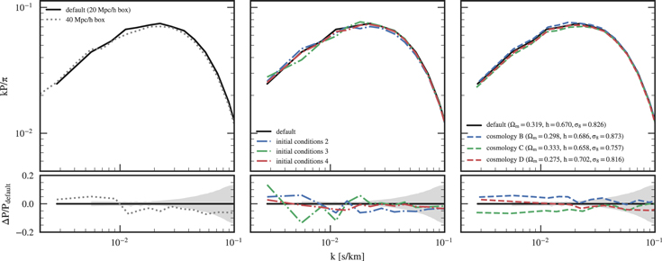
Figure 17. Left: one model from our thermal grid at z = 2.8 (solid black, the redshift is taken as an example, other redshifts are similar) compared to the same model run with a 2 times larger box and the same spatial resolution (dotted gray). The bottom panel shows relative differences and the size of the 68% confidence region of jointly fitting BOSS + high-resolution data as a gray band. Center: a comparison between different initial conditions (dotted-dashed) that were otherwise run with the same setup. Right: A comparison of models based on other cosmologies (B, C are compatible with the Planck Collaboration et al. 2016b parameters and chosen to maximally change the matter power spectrum w.r.t. the default model, see Oñorbe et al. 2017a for details; D is the cosmology from Lukić et al. 2015). We can see that all three effects change the power on the 5% level.
Download figure:
Standard image High-resolution image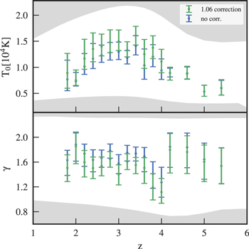
Figure 18. Comparison of our results on the thermal state with fits obtained if we apply a flat "correction factor" of 0.94 (mimicking the joint effect of box size and cosmic variance seen in Figure 17) to the model power (different colors). We can see that without the "correction" higher values of γ as well as lower values of T0 (due to correlations between parameters) are obtained.
Download figure:
Standard image High-resolution imageSimulations also suffer from statistical variance for the largest modes where the sampling is poor. To better understand this issue we ran simulations with different initial conditions but an otherwise identical setup. The comparison of those runs to our default simulation is shown in the middle panel of Figure 18. We can clearly see, that even with just four samples of initial conditions, a ∼5% change in the power can be reached on small scales similar to the results in the box size test above. Additionally, the effect of cosmic variance on the largest scales (lowest k ≲ 0.01  ) can exceed the 10% level, which is huge compared to the ∼2% errors of the BOSS measurement. To get both box size and cosmic variance effects under better control requires an analysis based on larger simulations, where doubling the (linear) box size would be expected to reduce cosmic variance by a factor of
  (but also needs at least 8 times more computing time).
To understand the effect of cosmological parameters on the Lyα forest power spectrum we compare to three different cosmologies consistent with the Planck Collaboration et al. (2016b) results. Cosmology B and C were selected from their posterior distribution in order to differ as much as possible in the linear matter power spectrum (see Oñorbe et al. 2017a). Cosmology D uses the same parameters as in Lukić et al. (2015). The right panel of Figure 18 shows that a change in cosmological parameters within the current CMB constraints can lead to a ∼5% change in the flux power as well. Of course a more detailed analysis of this effect is needed and ideally one would marginalize over cosmological parameters adding additional dimensions to our simulation grid. However, future independent higher precision cosmological constraints from either joining existing data sets or new measurements will reduce the strength of this effect.
Finally, the finite resolution of the simulations is not an issue at z ≲ 4 (see Figure 11 in Lukić et al. 2015, showing convergence to 1% at z ≤ 3 and to better than 5% at z = 4), but might be of some importance at z ≳ 5 (see the Appendix in Oñorbe et al. 2017a) and might be more severe in exceptionally cold models, as pressure smoothing is then weaker and structures are thus harder to resolve. In the latter case, the power at the smallest mode covered in our analysis could be underestimated at the ∼10% level, which is comparable to its error bars. However, in contrast to box size effects only the smallest scales ( ) are affected, which will not lead to changes as dramatic as seen for the other modeling errors considered in this section. However, the scale dependence of this effect, large scales (small k) being nearly unaffected, while small-scale power is reduced in the model, might lead to slightly underestimated results on T0.
In summary, we have seen that all four effects we discuss in this section, box size, initial conditions, cosmology, and resolution can affect the power spectrum by a similar amount as our statistical measurement errors at least for some range of scales and redshifts. We have seen that these effects can be comparable or larger than our statistical errors on the power spectrum, and can thus systematically change our thermal evolution at the 0.5–1σ level at a range of redshifts. Note again that all the effects we considered here are converged at the ∼5% level and a better treatment of any of the effects would require additional computation time or reduce the number of simulations that can be performed thereby increasing interpolation errors. The current analysis is therefore the best compromise between accurate results and available computing time. But note that the effects discussed here might very well explain some of the discrepancies between constraints of the thermal state obtained by different groups.
7. Conclusions and Outlook
In this work, we presented the first uniform thermal evolution analysis based on the Lyα forest power spectrum covering a large redshift range from z = 5.4 to z = 1.8 or equivalently a timespan of nearly 3 Gyr. For this purpose we combined multiple high-precision measurements performed by several groups using different instruments. Furthermore, we compared this data set with a large grid of high-resolution hydrodynamical simulations to connect the measured Lyα forest to physical properties of the IGM. To interpolate between these simulations we developed a GP emulation scheme and take its errors into account using a cross-validation approach. Compared to previous results we measure thermal evolution from high redshifts z = 5.4 to the limit of Lyα forest observability with ground-based telescopes due to the atmospheric UV cutoff at z ∼ 1.8, and our combination of high-precision low-k measurements with our new high-k analysis allows us to break the well-known degeneracy between the temperature at mean density and the slope of the TDR. Our analysis thus provides the first comprehensive homogeneous analysis of IGM thermal evolution probing times as early as the end stages of  reionization, extending through the epoch of
  reionization, and spanning the era of galaxy formation.
Our primary results are measurements of T0, γ, and λP (see Table 4) marginalizing over the mean transmission in two different ways (with a flat prior or a Gaussian prior based on recent measurements). These measurements show a clear increase in T0 from  at z = 5.4 to
  at z = 3.4 followed by a decrease reaching
  at z = 1.8. We compared our results to published thermal evolution constraints using different statistics and found broad consistency with data from curvature, Voigt profile fitting, and the phase angle distribution analyses. Comparing to simulations we indeed see compelling evidence for
  reionization in the rise of T0, which is not expected in absence of
  reionization. In general, the thermal parameters we obtained from fitting the power spectrum measurements agree well with models for which
  reionization is complete at z ∼ 3. At later times, i.e., z < 3, we see the first conclusive evidence that the IGM is cooling down after the last reionization heating episode driven by adiabatic cooling due to the expansion of the universe.
Table 4.
Fiducial Evolution of Thermal Parameters Assuming the Strong Prior on 
| z |

|
T0 | γ |

|

|

|

|
|---|---|---|---|---|---|---|---|
| (kpc) | ( ) ) |
( ) ) |
( ) ) |
||||
| 1.8 |

|

|

|

|

|

|
4.760 |
| 2.0 |

|

|

|

|

|

|
1.983 |
| 2.2 |

|

|

|

|

|

|
2.713 |
| 2.4 |

|

|

|

|

|

|
2.828 |
| 2.6 |

|

|

|

|

|

|
2.501 |
| 2.8 |

|

|

|

|

|

|
2.462 |
| 3.0 |

|

|

|

|

|

|
2.016 |
| 3.2 |

|

|

|

|

|

|
1.735 |
| 3.4 |

|

|

|

|

|

|
1.634 |
| 3.6 |

|

|

|

|

|

|
0.509 |
| 3.8 |

|

|

|

|

|

|
0.848 |
| 4.0 |

|

|

|

|

|

|
0.782 |
| 4.2 |

|

|

|

|

|

|
1.209 |
| 4.6 |

|

|

|

|

|

|
1.203 |
| 5.0 |

|

|

|

|

|

|
1.125 |
| 5.4 |

|

|

|

|

|

|
0.857 |
Download table as: ASCIITypeset image
However, at the highest redshifts z ≥ 5 we find evidence for low temperatures  (slightly higher, but consistent with other measurements based on the same data set) that might be hard to explain with our current understanding of the shape of the UVB at those redshifts as well as our current understanding of
  reionization. This is especially important as the same data set resulting in these low temperatures also places the most stringent limits on the mass of WDM (Viel et al. 2013). Comparing these power spectrum measurements to models that include both WDM particle mass as well as the IGM's thermal history as free parameters would necessarily result in an even colder IGM, because small-scale structure in the Lyα forest can now be erased by both thermal broadening and a finite WDM free-streaming length (see Figure 15, compare to Garzilli et al. 2017). Thus, given our current expectations for reionization heating, the cold temperatures we infer provide additional evidence for a cold DM universe.
To obtain a complete measurement of the IGM's thermal state, Lyα forest measurements clearly need to be extended to both higher and lower redshifts. At high z this would allow for testing the current power spectrum results and enable stronger joint constraints on the thermal state just after  reionization as well as the nature of DM (see Oñorbe et al. 2017b, for a forecast of possible constraints using high-resolution data up to z = 6) due to an increase in the available data set size in recent years. At the same time, the great success of the Cosmic Origins Spectrograph and Space Telescope Imaging Spectrograph on board the Hubble Space Telescope enables new measurements of the thermal state at low redshifts (
 ) allowing to test if the IGM cools down further as theoretically expected. As the post-reionization IGM physics is in principle well understood, these low-redshift measurements could then be used to constrain heat input from other astrophysical processes, e.g., galaxy formation or blazar heating.
However, to get precision constraints of the thermal state in the IGM, better hydrodynamical simulations are needed. We characterized the effect of box size, cosmic variance, and cosmology, and found that for some range of scales systematic uncertainties due to these effects can be comparable to our measurement precision. Future progress will therefore rely on simulating larger grids to marginalize over cosmological parameters or alternatively a more precise external determination of those parameters as well as larger simulation boxes. Thanks to great improvements in recent years, allowing nearly linear scaling of computing time with volume (at fixed resolution) in some hydrodynamical simulation codes, and the current advancement of computing speed in supercomputers, this will be possible within the next few years.
We thank Ashmeet Singh & Dan Foreman-Mackey for helpful discussions about Gaussian processes.
We thank Hector Hiss & Vikram Khaire for comments on the manuscript as well as all members of the ENIGMA group23 at the Max Planck Institute for Astronomy (MPIA) and University of California Santa Barbara (UCSB) for insightful suggestions and discussions.
Calculations presented in this paper used the hydra and draco clusters clusters of the Max Planck Computing and Data Facility (MPCDF, formerly known as RZG). MPCDF is a competence center of the Max Planck Society located in Garching (Germany). We also used resources of the National Energy Research Scientific Computing Center (NERSC), which is supported by the Office of Science of the U.S. Department of Energy under Contract No. DE-AC02-05CH11231.
Z.L. was supported in part by the Scientific Discovery through the Advanced Computing (SciDAC) program funded by the U.S. Department of Energy, Office of Advanced Scientific Computing Research and the Office of High Energy Physics.
Facilities: VLT/UVES (Dekker et al. 2000), Keck/HIRES (Vogt et al. 1994), SDSS-III/BOSS (Dawson et al. 2013), VLT/XSHOOTER (Vernet et al. 2011), Magellan/MIKE (Bernstein et al. 2003).
Software: emcee (Foreman-Mackey et al. 2013), george (Ambikasaran et al. 2016), NumPy (van der Walt et al. 2011), SciPy (Oliphant 2007), astropy (Astropy Collaboration et al. 2013), matplotlib (Hunter 2007), seaborn (Waskom et al. 2017), and Nyx (Almgren et al. 2013).
Appendix: Tables of the Measured Thermal Evolutions
In this appendix, we tabulate our measurement values at each redshift for the flat prior on  (Table 3) and the strong prior (Table 4). Those tables do not only show the marginalized constraints of all thermal parameters, but additionally show values for the temperature at the overdensity
  where curvature measurements are optimal (with the value for
  interpolated in redshift between results from Becker et al. 2011) as well as at
  where the degeneracy between γ and T is minimized for the power spectrum. The latter was obtained by assuming a power-law relation
  for the samples in our Markov chains and varying
  such that the variance of
  is minimized. The density values where degeneracies are minimal are tabulated as well. We will provide chains from our MCMC analysis on request.
Footnotes
- 6
- 7 is the redshift at which .
- 8
- 9
- 10
- 11
The exact number of models used is redshift dependent because of further cuts that are discussed at the end of this subsection.
- 12
If a low likelihood was achieved we optimized again using the downhill simplex method by Nelder & Mead (1965) and took the more optimal of the two runs.
- 13
In fact we discard all the different
realizations for this simulation in this test, as they all have the same thermal parameters. - 14
To be precise we demand
. As we have about 10 bins in γ, and about 7 in T0, the separation between adjacent points would be at least 0.1 in the units shown. But no two models have the same λP, increasing the separation. Therefore, the chosen minimal separation is still closer than our typical grid separation. While this threshold leads to good results throughout our redshift range, it is not necessarily the optimal one and further tests adopting different values could therefore be used to slightly increase interpolation accuracy. - 15
As the treatment of metal lines in the different data sets is following fundamentally different approaches, masking which should remove at least part of the
in the spectra versus subtraction of the metal power estimated from side bands, we decided to allow a different value for each measurement. Note that in the end thermal parameters will not be strongly correlated with the parameter. - 16
These values are also close to the formerly quoted "new values" from the instrument website as well as manuals until Period 101.
- 17
Based on our on estimates of XSHOOTER's resolution in Paper I, which is also close to the recently updated values on the XSHOOTER website and manual from Period 102.
- 18
Note that while we used DM models to correct the "raw" power in Walther et al. (2018), the masking correction performed here is fully based on hydrodynamical simulations.
- 19
We therefore show the extent of their 1σ contours (as a by-eye marginalization) for γ in Figure 15.
- 20
Notice that the interpretation of the duration of reionization in homogeneous UVB models can be misleading. We point to Oñorbe et al. (2017a) for a full discussion in this regard.
- 21
We note that this reionizes
slightly earlier z = 7.3, which is still in good agreement with both Planck results. - 22
Note that the initial conditions cannot be the same for two boxes of different size, and so every comparison of this kind includes cosmic variance on both boxes, but with
times lower amplitude at a given mode for the larger box. - 23


