


Abstract
Low-frequency radio observations make it possible to study the solar corona at distances up to 2–3 R☉. Frequency of plasma emission is a proxy for electron density of the emitting plasma and, therefore, observations of solar radio bursts can be used to probe the density structure of the outer corona. In this study, positions of solar radio sources are investigated using the Low-Frequency Array (LOFAR) spectral imaging in the frequency range 30–50 MHz. We show that there are events where apparent positions of the radio sources cannot be explained using the standard coronal density models. Namely, the apparent heliocentric positions of the sources are 0.1–0.7 R☉ further from the Sun compared with the positions predicted by the Newkirk model, and these shifts are frequency-dependent. We discuss several possible explanations for this effect, including enhanced plasma density in the flaring corona, as well as scattering and refraction of the radio waves.
Export citation and abstract BibTeX RIS

Original content from this work may be used under the terms of the Creative Commons Attribution 3.0 licence. Any further distribution of this work must maintain attribution to the author(s) and the title of the work, journal citation and DOI.
1. Introduction
Most observations of the solar atmosphere are limited to the lower corona, where the ambient plasma density and magnetic field are sufficiently high to produce substantial fluxes of X-ray, extreme ultra-violet, and microwave emissions, which can be used for diagnostics of thermal and nonthermal plasma components. However, observational diagnostics of the outer corona (at ∼1 R☉ and higher) are quite problematic due to very low plasma density. Energetic electrons propagating through the solar corona and heliosphere result in the generation of plasma waves, which, in turn, produce coherent radio emission at and above the local plasma frequency, from ∼1 GHz in the lower corona to few megahertz in the outer corona (see, e.g., Ginzburg & Zhelezniakov 1958; Kundu 1965; Takakura 1967; Melrose 1980, for review). Since plasma frequency is determined by the local electron density, this type of radio-emission is extremely important for probing the properties of thermal plasma and dynamics of energetic particles in the outer corona. The dynamic frequency spectra of the coherent plasma emission make it possible to deduce parameters of the nonthermal plasma, such as energetic electron velocities (e.g., Aschwanden et al. 1995; Krupar et al. 2015). Solar radio observations with both spatial and spectral resolution substantially enhance diagnostics opportunities, making possible simultaneous diagnostics of the nonthermal and thermal plasma components in the coronal plasma (e.g., Bastian et al. 2001; Pick & Vilmer 2008; Kontar et al. 2017b).
Starting from the late 1950s, there have been a number of studies concerning the heights of the solar low-frequency radio bursts (e.g., Wild et al. 1959; Stewart 1976; Dulk & Suzuki 1980; Leblanc et al. 1998). The new generation of low-frequency radio arrays, such as the Murchison Widefield Array (MWA; Oberoi et al. 2011) and the LOw-Frequency ARray (LOFAR; van Haarlem et al. 2013), provide a unique opportunity for mapping solar radio sources with very high temporal and spectral resolution, making possible a detailed study of the coronal density structure. However, the solar corona is not fully transparent for the low-frequency radio waves. Plasma inhomogeneities, which should be ubiquitous in the corona, may interact with propagating radio waves, resulting in scattering and refraction. They, in turn, may result in a substantial shift of an apparent radio source position.
Early positional observations of the sources in solar radio bursts showed that solar low-frequency sources often appear further away from the Sun than expected based on their frequencies. This effect was interpreted as a result of enhanced density in the corona over the active regions (e.g., Wild et al. 1959; Bougeret et al. 1984). However, it has also been suggested that scattering and refraction of radio waves in the corona can substantially affect apparent source positions (e.g., Fokker 1965; Aubier et al. 1971; Robinson 1983; Bastian 1994). More recently, based on a spectral imaging study of a type III source with LOFAR, Kontar et al. (2017b) suggested that refraction and scattering might be the dominant factors determining apparent positions and sizes of LOFAR sources. Thus, a recent study by Chrysaphi et al. (2018) demonstrated that apparent positions of solar radio sources are consistent with the presence of strong radio-wave scattering. Another recent study, by McCauley et al. (2018), also shows that coronal density enhancement cannot fully explain positions of radio sources in some type III radio-bursts observed with MWA radio array in the range of 80–240 MHz.
In this study we investigate frequency–distance (FD) structure of the low-frequency sources observed by LOFAR in several solar radio bursts. Observations of the Tau A radio source are used to evaluate the error of positional measurements with LOFAR (Section 2). Then, by treating the projection angle as a free parameter, we compare the heliocentric distances of several radio sources with distances predicted by various standard coronal density models (Section 3). We also investigate the potential effect of radio-wave scattering in the corona on apparent positions of the observed sources using the approximate analytical approach developed by Chrysaphi et al. (2018; Section 4).
2. Observations and Data Analysis
This study is based on the analysis of 12 apparent radio sources observed in 9 solar radio events, randomly selected from the set of radio bursts observed during two solar LOFAR observational campaigns. The observational data were obtained in a tied-array beam-forming mode (van Haarlem et al. 2013) with 24 core LOFAR stations allowing a maximum baseline of around 3.5 km, providing beam sizes of about 580 and 350 arcsec at 30 and 50 MHz, respectively. We use observations with 172 beams (in 2015) and 217 beams (2017). The number of beams is limited by computational capabilities of the instrument. Beam sensitivities were calibrated using observations of a known source; namely, by measuring Tau A flux using one of the beams constantly pointing at it. In addition to single-beam Tau A observations, a number of spatially resolved Tau A observations have been performed using the same configuration of the beam array as in solar observations.
For one of the studied events (2015 June 25, see Section 4), simultaneous observations with URAN-24 (Megn et al. 2003) have been used for cross-calibration of the total solar flux as well as polarization. Furthermore, the data from the Nançay Decametric Array (NDA; Boischot et al. 1980; Lecacheux 2013) have been used to evaluate polarization in two of the considered events (2015 June 20 and 25).5
Table 1 shows basic information about the observed events. Five of the events demonstrate features typical for type III radio bursts: short duration (several minutes), negative frequency drift of  with df/dt decreasing with time. There are also four long-duration events with two exhibiting features typical for type II bursts and two with the dynamic spectra typical for type IV events.
Table 1. Characteristics of the Considered LOFAR Sources
| Event and Source Number | Date and Time (UT) | Elevation | Frequency Range, MHz |
|---|---|---|---|
| Sun | |||
| L340180 | 2015 Apr 16 11:56 | 47° | 30–45 |
| L341082 | 2015 Apr 16 13:08 | 44° | 45–55 |
| L342370 | 2015 May 6 11:47 | 54° | 30–45 |
| L346964 (S1) | 2015 Jun 20 11:10 | 60° | 30–45 |
| L346964 (S2) | 2015 Jun 20 11:10 | 60° | 35–55 |
| L346964 (S3) | 2015 Jun 20 11:10 | 60° | 35–50 |
| L347538 | 2015 Jun 25 11:08 | 61° | 30–45 |
| L599747 (S1) | 2017 Jul 12 08:52 | 45° | 30–45 |
| L599747 (S2) | 2017 Jul 12 08:52 | 45° | 35–50 |
| L599749 | 2017 Jul 13 07:08 | 31° | 30–45 |
| L599761 | 2017 Jul 15 11:01 | 58° | 35–50 |
| L608616 | 2017 Sep 9 11:43 | 43° | 30–50 |
| Tau A | |||
| L599361 | 2017 Jul 06 16:20 | 15° | 35–50 |
| L599635 | 2017 Jul 09 10:02 | 59° | 35–50 |
| L608614 | 2017 Sep 9 10:05 | 34° | 35–50 |
Download table as: ASCIITypeset image
In all events considered in this study, radio emission appears in a rather narrow frequency range with Δf/f ≃ 0.2–0.5 (see dynamic spectra in Section 4). This seems inconsistent with the gyrosynchrotron mechanism, which is sometimes used to explain lower-frequency radio emission, particularly during type IV bursts (Ramaty 1969; Dulk 1973). Furthermore, observed sources have high brightness temperatures, which is not typical for the gyrosynchrotron mechanism. Therefore, most likely, the observed emission is produced by the plasma mechanism.
Observed source positions are calculated using three different methods: using locations of the intensity maxima of the sources, using centers-of-mass of the intensity maps of the sources with the intensity threshold of 0.5 of their maximum intensity, and using two-dimensional elliptical Gaussian fitting with the intensity threshold of 0.5 of the corresponding source maximum intensity. All three methods yield very close values (see Section 3), indicating that the observed sources normally have rather symmetric, elliptical shapes.
In order to estimate the error of centroid position measurements and to evaluate the effect of the ionospheric refraction, we initially use three sets of Tau A observations at different zenith angles. Figure 1 shows Tau A intensity maps at four different frequencies during one of the observations. At frequencies 30–50 MHz the maps demonstrate patterns typical for interferometric observations: one bright source and several fainter sources, which are side-lobes. The position of the main lobe does not shift significantly with frequency. However, at frequencies higher than 50–55 MHz the picture becomes very complicated with some of the side-lobes being brighter than the main lobe. Analysis of this effect is beyond the scope of this study; however, in this manuscript we only use observations in the frequency range of 30–50 MHz.
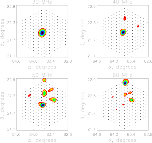
Figure 1. Tau A intensity maps observed by LOFAR 10:02 UT on 2017 July 9 at four different frequencies. The object elevation was 59° over horizon.
Download figure:
Standard image High-resolution imageFigure 2 shows centroid positions of Tau A measured at different frequencies, from 30 to 50 MHz. It can be seen that the measured centroid positions (black symbols) can differ substantially (by up to 1000–1500 arcsec) from the actual position of the object. This difference is bigger for lower elevations, indicating that it is caused mostly by the ionospheric refraction. To correct for this effect, we use a simple formula:
where  , z is zenith angle in degrees (z = 90° − E, where E is the elevation angle). This formula is based on derivations shown in Thompson et al. (2017), the coefficient is chosen to minimize the dispersion of Tau A centroids in observations above 30° over horizon (Figures 2(b) and (c)). Because this formula ignores any seasonal or daily variations, this correction is valid for "average" ionospheric conditions and cannot completely remove the ionospheric refraction shifts in individual observations. However, in this study, we consider solar observations with elevations of at least 30° and, hence, the above formula can be used for the ionospheric refraction correction.

Figure 2. Locations of Tau A centroids measured using LOFAR data. Panels (a)–(c) show centroids of Tau A for three different sets of observations at different frequencies. The black ellipse schematically shows position and dimensions of the Tau A radio source, with  and
and  . Black symbols show measured centroid positions. They are linked to color symbols showing centroid positions calculated taking into account the ionospheric refraction correction. Colors denote different frequencies, from 30 MHz (red) to 48 MHz (blue). Elevations of Tau A for corresponding events are given above the panels. (In panel (c) gray and color symbols nearly coincide.)
Download figure:
Standard image High-resolution imageCorrected centroid positions (color symbols in Figure 2) appear much closer to the actual position of Tau A. Although the refraction correction "brings" centroid positions closer to the expected location, the spread of points is still very significant for low elevation observation (Figure 2(a)), indicating that our approximate formula cannot be used for the sources observed low over the horizon. Furthermore, there are other factors that contribute to the spread of the centroid positions, including the instrumental errors (due to finite size of the beam, effect of faint sidelobes, etc.) and data processing errors (e.g., centroid fitting error).
In order to evaluate the error of position measurements we use two sets of Tau A observations at elevations of 34° and 59°. Based on the spread of positions at different frequencies and the distance between measured and expected Tau A positions, we conclude that the error is approximately 150 arcsec or 0.15 R⊙, which is used as an error bar in Figures 3–6.

Figure 3. Intensity map and frequency–distance diagrams of the source observed at UT = 11:01 on 2017 July 15. The intensity map (panel (a)) is for 42 MHz. The red arrow points at the considered source. Three other panels (b)–(d) show FDD for different projection angle values. Red line, and purple and green symbols in panel (b) correspond to positions measured using centers-of-mass, intensity maxima, and 2D elliptical Gaussian fitting. Solid black lines show heliocentric distances of sources of fundamental plasma emission expected from the Newkirk density model of the corona (Newkirk FDD). Dashed black lines show FDDs corresponding to the models with densities lower by a factor of 2 and higher by a factor of 2 compared to the Newkirk model. Solid and dashed blue lines show apparent distances of sources predicted by the density models denoted by black lines, but shifted due to scattering (see Section 4 for details).
Download figure:
Standard image High-resolution image3. Results
3.1. Frequency–Distance Diagrams
Let us calculate the expected radio-emission frequencies and compare them with frequencies of the observed LOFAR sources at different heliocentric distances. If the emission is produced at the local fundamental plasma frequency, then its frequency depends on local electron density as

Average densities in the outer corona are expected to follow the Newkirk density model (Newkirk 1961, 1967):

Using this density model it is possible to relate fundamental emission frequencies with heiocentric distances:

The observed elongations of sources from the solar disk center  are related to their heliocentric distances as

which is equivalent to the projected heliocentric distance robs

i.e., to the projection of the heliocentric distance on the plane of the sky. Here L is the distance between the Earth and the Sun and θ is the projection angle, i.e., the angle between the heliocentric direction of the source and the line of sight, which is not known. Hence, real heliocentric distances of the sources are calculated for a range of the projection angles from 90° to 20°. This yields a set of source positions corresponding to a set of frequency values—the so-called FD diagrams (FDDs). These diagrams are calculated for different projection angles and compared with the FDD predicted by the Newkirk model (Equation (3), Newkirk FDD thereafter). Below, FDDsof the observed solar radio sources that can fit Newkirk FDD at some projection angle are called normal FDDs, while those showing substantial deviations at any position angle are called abnormal FDDs.
Figures 3–6 demonstrate FDDs for four different sources, compared to the FD curves expected from the Newkirk density model. The times, corresponding to these intensity maps and FDD were chosen randomly. However, we found that these diagrams normally do not show substantial variations during the lifetime of these sources. The projection effect shifts FDDs to higher apparent heliocentric distances and reduces their gradients. The projection effect is also taken into account in error calculations: error bars become longer at lower projection angles. Figure 3 demonstrates FDDs for one of the sources for three different values of the projection angle, showing relatively good agreement with the Newkirk coronal model for θ ≈ 80°–90°. Eight of 12 considered sources demonstrate similar FDDs, i.e., they can fit Newkirk's FD curves at some projection angle. However, at least 3 of 12 considered sources show deviations from the FD curves expected from the Newkirk density model, which are bigger than the error and cannot be explained by the projection effect. Below we discuss each of these sources.
3.2. 2015 June 20 Event
The LOFAR dynamic spectrum (Figure 7(a)) for this event reveals a type IV burst starting around 11:00 UT and continuing over two hours. Almost simultaneously with this radio-event a coronal mass ejection (CME) was observed by SOHO LASCO coronograph in white-light off the northeast limb at the position angle of 39°, starting around 11:00 UT (see SOHO/LASCO CME catalog6 ), which is possibly associated with the observed radio burst.
LOFAR intensity maps of this event demonstrate three distinct apparent sources forming a loop-like structure (Figure 4(a)). Two sources appear relatively close to the solar disk: the source off the eastern limb, which dominates at frequencies below 40 MHz, and the source off the northern limb, dominating at ∼50 MHz. The lower-frequency source shows normal FDD, which fits the Newkirk density model at the projection angle 55°–60°. However, the higher frequency source demonstrates an abnormal FDD: it decreases slower than the Newkirk FD function, i.e., at lower frequencies this source appears significantly further from the Sun than expected (Figures 4(b)–(d)). Thus, the apparent heliocentric distances of its centroids at 45–50 MHz are consistent with those predicted by the Newkirk density model, while centroids at 35–40 MHz are located about 0.15–0.20 R⊙ further than expected from the Newkirk model, which is larger than the positional error (see Section 2). It is important that the FD function is relatively smooth and the value of deviation from the Newkirk FD function gradually increases with decreasing frequency, showing that this abnormality is not a result of a stochastic measurement error.

Figure 4. Same as in Figure 3 but for the source off the N limb observed at UT = 11:10 on 2015 June 20. The intensity map is for 48 MHz.
Download figure:
Standard image High-resolution imageThe third source, dominating at frequencies between ∼40 and 50 MHz, also has abnormal FDD: it appears much further (by ∼1 R⊙) than expected. However, it is located too close to the field-of-view boundary and, therefore, it is impossible to make any conclusive measurements for this source.
3.3. 2015 June 25 Event
This event has been recently studied in detail by Chrysaphi et al. (2018). Its has a dynamic spectrum typical for type II radio-bursts followed by a number of type III-like bursts (Figure 7(b)), and is associated with the CME eruption, which has been observed in close spatial and temporal proximity by the LASCO coronograph. LOFAR intensity maps of this event reveal emission in the frequency range 30–45 MHz off southwest limb of the solar disk (Figure 5(a)). Chrysaphi et al. (2018) focused on the band-splitting stage (∼10:45–11:00 UT) and demonstrated that apparent positions of the radio source observed at different frequencies is consistent with the coronal shock configuration, with the sources strongly shifted due to radio-wave scattering.

Figure 5. Same as in Figure 3 but for the source off the SW limb observed at UT = 12:08 on 2015 June 25. The intensity map is for 38 MHz.
Download figure:
Standard image High-resolution imageIn this study we investigate this event between 11:00 and 12:00 UT. During this time the dynamic spectrum for this event reveals a number of type III-like fibrils in the frequency range 30–45 MHz with a typical duration of 10 s. FD measurements during this stage of this event show abnormal FDDs. Figure 5 shows FDDs corresponding to one of the fibrils at 11:08 UT. Similar to Chrysaphi et al. (2018), we find that the source is located noticeably further than predicted by the Newkirk density model. Furthermore, similar to the 2015 June 20 event (Section 3.2), the FD function for this event decreases substantially slower than expected. Thus, the location of centroids at 40–45 MHz can be explained by the Newkirk density model multiplied by a factor of 2–2.5. However, this factor gradually increases toward lower frequencies, and the locations of centroids at 30–35 MHz can be explained by the Newkirk density model multiplied by factor of 4–4.5. This transition is gradual, i.e., centroid positions during the considered time interval cannot be explained by a Newkirk density model multiplied by a single factor.
3.4. 2017 July 12 Event
Similar to the 2015 June 20 and 25 events, this event is also a long-duration event. Its dynamic spectrum (Figure 7(c)) consists of a number of fibrils, typically 3–5 s long, demonstrating both negative and positive frequency drifts.
LOFAR observations of this event reveal two relatively bright sources (Figure 6(a)). The first source, located off the southeast limb, produces emission in the ∼30–45 MHz range. The second, fainter source is located off the northeast limb and is visible in the ∼35–50 MHz range. At first glance, the fainter, northeast source seems to be a side-lobe produced by the brighter, southeast source. However, a more detailed analysis shows that this is a separate source. First, the distance between these two sources measured at different frequencies does not vary as 1/f, as it is expected for a side-lobe. Second, the relative brightness of the NE source is higher compared to the sidelobes of our calibration source, Tau A. Finally, the dynamic spectrum of the NE source is different from that of the SE source.
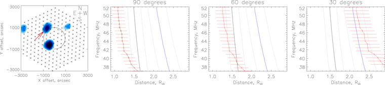
Figure 6. Same as in Figure 3 but for the source off the NE limb observed at UT = 08:52 on 2017 July 12. The intensity map is for 43 MHz.
Download figure:
Standard image High-resolution image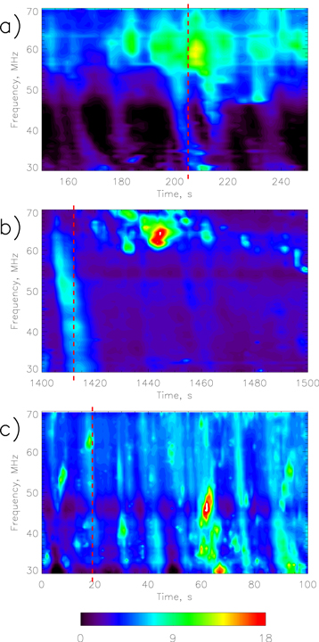
Figure 7. LOFAR dynamic spectra for the three events discussed in Sections 3.2–3.4. Red dashed lines show the moments corresponding to the intensity maps and FD diagrams in Figures 4–6. Panel (a) is for the 2015 June 20 event, the horizontal axis shows time after 11:07:00 UT. Panel (b) is for the 2015 June 25 event, the horizontal axis shows time after 11:45:00 UT. Panel (c) is for the 2017 August 12 event, the horizontal axis shows time after 08:51:14 UT. Note that axes have different scales in different panels.
Download figure:
Standard image High-resolution imageThe NE source demonstrates abnormal FDD (Figures 6(b)–(d)): similar to the two previous events discussed, its FD function decreases slower with apparent heliocentric distance. Thus, in the range of 42–52 MHz the source position is close to that expected from the Newkirk density model with the projection angle of about 50°–55°, though the FD function is less steep than the Newkirk FD function. However, in the frequency range 37–42 MHz the FD function of this source becomes even flatter, and its shape cannot be explained by any reasonable projection angle.
4. Discussion
The abnormal FD structure of the three sources discussed in Sections 3.2–3.4 cannot be explained by the geometric effects. The projection effect, obviously, can only increase the real heliocentric distance, because rsrc ≥ robs (see Section 3.1). Furthermore, it cannot be explained by the source curvature, for instance, due to the electron beam propagating along highly curved magnetic field lines. It is easy to show that the curvature can only steepen the slope of an FD function (see, e.g., Lobzin et al. 2010).
There are several mechanisms that can potentially explain the observed effect. First, it can be due to the electron density in the outer corona being substantially different from the Newkirk density model, which describes average coronal conditions. Assuming that the sources are produced by fundamental plasma emission and their apparent positions are not shifted by some propagation effects, one can evaluate the plasma densities in the considered events, as well as the hydrodynamic scale lengths,  . Thus, while the average heights of the sources observed on 2015 June 20 and 2017 July 12 (discussed in Sections 3.2 and 3.4, respectively) can be approximated by the Newkirk density model with the projection angles of about 90° and 50°–55°, respectively, their FD functions yield hydrodynamic scale lengths of 0.7 and 1.3 R⊙, which are much longer than that in the Newkirk density model, ∼0.3 R⊙. The average height of the source observed on 2015 June 25 (Section 3.3) requires densities from the Newkirk model multiplied by a factor of 2.5–4.5 with the projection angle of 90°; the shape of FD function of this source corresponds to the hydrodynamic scale length of about 1 R⊙.
Obviously, the three radio sources described in Section 3 are associated with active events in the corona, with two of them following CME eruptions. Fast energy release during solar flares and eruptive events can lead to major changes in the corona: fast plasma flows and large-scale turbulence can enhance coronal density and increase the hydrodynamic scale length (see, e.g., simulations by Gordovskyy et al. 2014).
Another possibility is that apparent source positions are shifted either due to radio-wave scattering or refraction. Turbulence should be present in the corona following major energy release events; various theoretical models and observational estimations show that turbulence contains order of 10−2 of the energy released in flares (see, e.g., Bornmann 1987; Gordovskyy et al. 2016; Kontar et al. 2017a). Coronal density perturbations due to plasma turbulence would result in scattering of propagating radio waves and, hence, in the increased sizes and shifted positions of the radio sources. Kontar et al. (2017b) analyzed the type III radio-burst observed by LOFAR on 2015 April 16 and concluded that the observed source sizes can only be explained by the presence of strong radio-wave scattering. In fact, they suggest that scattering is likely to be the main mechanism defining the apparent heliocentric positions of the radio-sources observed in this frequency range. Chrysaphi et al. (2018) show that the positions of the radio-sources during the band-splitting stage of the 2015 June 25 event are consistent with the effect of radio-wave scattering. They also propose a simplified method of estimating the effect of radio-wave scattering by local density inhomogeneities caused by plasma turbulence.
The method proposed by Chrysaphi et al. (2018) treats radio-wave scattering in a manner similar to the scattering of a charged particle in plasma: photons traveling through the corona undergo repeated small-angle (dθ) deflections due to varying plasma density, these deflection angles are proportional to the variations of plasma density δn/n. The mean scattering rate  should depend on the mean variation of the plasma density experienced by photons,
  . Here
  denotes ensemble average; θ2 is a solid angle. The scattering per unit distance is related to the scattering rate through the group velocity vgr as
  . Hence, it can be shown that the mean scattering of a radio-wave frequency f0 propagating in plasma with local frequency f(r) per unit length should be
where  is the normalized mean power of plasma turbulence and H is typical density inhomogeneity correlation length. The LHS term in the above equation characterizes radio-wave scattering and decay in respect to the propagation direction, and is effectively similar to the extinction coefficient in the radiative transfer equation. Hence, similar to the radiative transfer in the photosphere, one can introduce the optical depth with respect to the scattering for radio-waves propagating in the corona:

where  . Radio waves should propagate diffusively where τ > 1 and freely where τ < 1. Hence, their apparent positions will correspond to heliocentric distances where τ ≈ 1 for a given frequency.
FD functions showing positions of sources generated in the corona with the Newkirk density model and shifted by plasma turbulence (as per Equations (6)–(7)) are shown in Figures 3–6 (panels (b)–(d)). These functions are calculated assuming that  (the fraction of energy, supposedly, carried by the turbulence), and the typical correlation length is H ≈ 1 km (which, by order of magnitude, corresponds to an average Larmor radius of ions in magnetic field of ∼1 G at ∼1 MK). It can be seen that turbulent scattering with the assumed parameters results in substantial shifts of apparent source positions: Δr is about 0.5 R⊙ at 50 MHz, increasing to about 0.8 R⊙ at 30 MHz. Furthermore, the obtained FD functions are less steep, compared to the FD expected from the Newkirk density model. Therefore, scattering can, indeed, explain larger than expected heliocentric distances of solar radio sources, and, to some extent, can explain shapes of FD functions (i.e., the apparent hydrodynamic scales).
Finally, it might be considered that the observed sources can be produced by the harmonic plasma emission. For instance, the N = 2 harmonic would produce the same FD function as the density model multiplied by a factor of 4. This can potentially explain larger than expected apparent heliocentric distance, like one in the 2015 June 25 event. However, the dynamic spectra for the 2015 June 20 and 25 obtained using NDA show that the emission in these two events is strongly polarized. In both events the polarization degree is up to ∼70%–80%, then decreases to 20%–40%. This high degree of polarization is usually assumed to be inconsistent with the harmonic plasma emission (see, e.g., Dulk & Suzuki 1980; Dulk et al. 1984). Furthermore, harmonic emission would not be able to explain flatter than expected FD functions. Therefore, although the harmonic emission cannot be completely ruled out, it is unlikely to be the main factor behind the observed effect.
The Newkirk model is one of the "canonical" coronal density models used in solar radio-astronomy. Other widely used models include van de Hulst, Baumach–Allen, and Saito models (Figure 8; see, Allen 1947; van de Hulst 1950; Saito 1970, respectively). However, these models predict even lower coronal densities between 1 and 4 R⊙, and, therefore, are less able (compared to the Newkirk model) to explain the apparent source positions (see Section 3).

Figure 8. Density models of the solar corona compared to the Newkirk model (solid black line). Blue dotted line is for Saito (1970) model, green dashed line is for van de Hulst (1950) model, and red dotted–dashed line is for Baumbach–Allen model (Allen 1947).
Download figure:
Standard image High-resolution image
Therefore, we conclude that the observed effect (shown in Figures 4–6) is likely to be caused by a combination of the density changes in the active corona and the scattering of radio-emission due to plasma turbulence. It is practically impossible to estimate contributions of each of these two effects at this point. One possible way to overcome this problem might be using additional observational constraints (such as simultaneous measurement of apparent source sizes and positions) and comparing them with the theoretical models of radio-wave propagation. In any case, based on these results and previous observational studies, we can conclude that radio-wave propagation effects, such as scattering, can shift apparent source positions by ∼0.1–1 R⊙ and, hence, the FD relation following from a theoretical coronal density model (such as the Newkirk model) cannot be used to estimate real heliocentric distances of the sources and the projection effect.
5. Summary
In this study we analyze image-spectroscopic LOFAR observations of solar radio bursts in the frequency range 30–50 MHz. Based on the frequencies of the observed sources, electron densities in outer corona are estimated assuming that these LOFAR sources are produced by plasma emission. The estimated densities are compared with canonical coronal density models. Based on this analysis, we find at least three events where radio sources have apparent positions substantially different from those predicted by the Newkirk density models. Thus, they appear further from the Sun, confirming some earlier observations (e.g., Stewart 1976; McCauley et al. 2018). Furthermore, we find that their lower-frequency centroid positions (at 30–35 MHz) are shifted even further than their higher frequency centroids (at 40–50 MHz. These features cannot be explained by the projection, curvature, or any other geometric effect.
There are three possible explanations for this effect:
- (a)denser and less stratified coronal plasma,
- (b)sources are produced by harmonic plasma emission, and
- (c)radio-wave scattering due to plasma turbulence.
Based on our analysis and previous studies, we conclude that the observed effect is caused by a combination of actual density changes and strong radio-wave scattering due to plasma turbulence in the active corona.
It is difficult to say what proportion of solar radio sources demonstrate abnormal heliocentric distances because of the uncertainty due to unknown projection angle. Statistical analysis would be the most optimal way of overcoming the uncertainty due to projection effect: the distribution of the radio sources in respect of apparent heliocentric distance can be derived for a large number of sources assuming that their distribution is spherically symmetric. However, 102–103 sources would be required to make such an analysis statistically representative.
This work was funded by the Space and Technology Facilities Council (UK), grants ST/L000768/1 (M. Gordovskyy and P.K. Browning) and ST/L000741/1 (E.P. Kontar). A.A.K. acknowledges partial support from the RFBR grant 17-52-10001 and base financing of FR program II.16.
This paper is based (in part) on data obtained from facilities of the International LOFAR Telescope (ILT) under project codes LC3_012 and LC4_016. LOFAR (van Haarlem et al. 2013) is the Low Frequency Array designed and constructed by ASTRON. It has observing, data processing, and data storage facilities in several countries that are owned by various parties (each with their own funding sources), and that are collectively operated by the ILT foundation under a joint scientific policy. The ILT resources have benefited from the following recent major funding sources: CNRS-INSU, Observatoire de Paris and Université d'Orléans, France; BMBF, MIWF-NRW, MPG, Germany; Science Foundation Ireland (SFI), Department of Business, Enterprise and Innovation (DBEI), Ireland; NWO, The Netherlands; The Science and Technology Facilities Council, UK; Ministry of Science and Higher Education, Poland. The authors acknowledge the support by the international team grant (http://www.issibern.ch/teams/lofar/) from ISSI Bern, Switzerland.
Footnotes
- 4
URAN-2 data are available at http://cesra.net/?page_id=187.
- 5
NDA data are available online http://www.obs-nancay.fr/-Reseau-decametrique-24-.html.
- 6