


Abstract
Observations with the Goode Solar Telescope (GST) are presented here showing that the emergence of 1.91 × 10¹⁸ Mx of new magnetic flux occurred at the edge of a filamentary light bridge (LB). This emergence was accompanied by brightness enhancement of a photospheric overturning convection cell (OCC) at the endpoints of the emerging magnetic structure. We present an analysis of the origin and the dynamics of this event using high-resolution GST Fe i 1564.85 nm vector magnetic field data, TiO photospheric, and Hα chromospheric images. The emerged structure was 1.5 × 0.3 Mm in size at the peak of development and lasted for 17 minutes. Doppler observations showed presence of systematic upflows before the appearance of the magnetic field signal and downflows during the decay phase. Changes in the orientation of the associated transverse fields, determined from the differential angle, suggest the emergence of a twisted magnetic structure. A fan-shaped jet was observed to be spatially and temporally correlated with the endpoint of the OCC intruding into the LB. Our data suggest that the emerging fields may have reconnected with the magnetic fields in the vicinity of the LB, which could lead to the formation of the jet. Our observation is the first report of flux emergence within a granular LB with evidence in the evolution of vector magnetic field, as well as photosphere convection motions, and supports the idea that the impulsive jets above the LB are caused by magnetic reconnection.
Export citation and abstract BibTeX RIS
1. Introduction
Light bridges (LBs) are elongated, bright, granular structures that divide the umbra of a sunspot into two or more umbral regions with the same or the opposite magnetic polarities (Muller 1979; Zirin & Wang 1990; Sobotka et al. 1994). The magnetic field in LBs is weaker than that in the sunspot umbra, and the convective motions of plasma inside LBs are not totally inhibited (e.g., Lagg et al. 2014). Simulation results indicate that field-free plasma from the underlying convection zone contains more than enough internal energy to penetrate into the umbra along openings in the magnetic field, and that it can reach the solar surface manifesting itself as LBs of various thickness and length (Schüssler & Vögler 2006). LBs can be categorized as faint, strong, or granular depending on their brightness, size, and the internal structure. The magnetic field of all types of LBs show a similar pattern of increasing field strength with height, and a cusp-like configuration (Jurčák et al. 2006). Recent observations showed that granular LBs are quite similar to quiet Sun granulation (Lagg et al. 2014).
Solar jets, characterized as impulsive evolution of well-collimated bright or dark structures that extend along a particular direction, occur commonly in the upper solar atmosphere. The observed spatial scale of jet-like events ranges from the limits of telescope resolution to hundreds of megameters, and they can be detected in all available spectral ranges (e.g., Pariat et al. 2015, 2016). Kurokawa (1988) and Kurokawa & Kawai (1993) reported that Hα jets often appear at the earliest stage of magnetic flux emergence (MFE) and could continue for many hours. They suggested that the essential mechanism for producing these Hα jets is likely to be magnetic reconnection between a newly emerging flux and a preexisting magnetic field. Yokoyama & Shibata (1995) further showed in their numerical simulation that such reconnection might indeed produce Hα surges in emerging flux regions.
Chromospheric jets are commonly seen above LBs. Ejected plasma is normally observed rooted between one side of a LB and the adjacent umbra, and moving upward along the magnetic field above the LB (Asai et al. 2001; Louis et al. 2014). Those authors stated that the jets suggest the emergence of a bipolar magnetic flux or the presence of opposite polarity field. Bharti et al. (2007) reported evidence of opposite polarity fields emerging in a LB followed by a cospatial plasma ejection event. Louis et al. (2015) reported observational evidence of a small-scale Ω loop that emerged in a LB and led to a chromospheric brightening. Recently, Toriumi et al. (2015a, 2015b) showed that chromospheric brightenings and dark surges in a LB are a consequence of magnetoconvective evolution within the LB interacting with the surrounding magnetic fields. Tian et al. (2018) categorized surge-like activities above the LBs into oscillation-driven surges and reconnection-triggered jets.
An alternative explanation of the LB jets is that they are the result of shocks generated by magnetic reconnection or photospheric waves. Yurchyshyn et al. (2014) reported detailed observations of umbral jet-like structures, and demonstrated they might be driven by upward propagating shocks generated by photospheric oscillations. Bharti (2015) and Yang et al. (2015) recently reported on a bright front ahead of a system of Hα jets above LB that were coherently oscillating in vertical direction. Bharti (2015) further noted that magnetic reconnection fails to fully explain the coordinated behavior of these oscillating jets, while Yang et al. (2015) interpreted the oscillating light wall, which is the counterpart of the LB in the chromosphere, as a leakage of p-mode waves from below the photosphere. These oscillations were also found to be enhanced or suppressed by external disturbances such as flares (Hou et al. 2016; Yang et al. 2016). Song et al. (2017) observed shock waves, generated by magnetic reconnection between an emerging flux inside a LB and the adjacent umbral magnetic field, that were driving arcsecond-scale plasma ejections above a LB. Zhang et al. (2017) reported that surge-like oscillations above LBs resulted from p-mode shock waves transmitted from the photosphere.
Penumbral microjets (PJs) are finescale, jet-like features ejected in the chromosphere above a penumbra and they could be triggered in the same way as the LB jets. PJs were first reported by Katsukawa et al. (2007) using data from the Solar Optical Telescope/Filtergraph (SOT/FG; Ichimoto et al. 2008) on board the Hinode satellite (Kosugi et al. 2007). Magnetohydrodynamic (MHD) simulations support the idea that reconnection drives these events by inducing strong plasma outflows along horizontal flux tubes (Sakai & Smith 2008) or by assuming the horizontal field in a twisted flux tube (Magara 2010). The convective upflows continuously transport magnetic fields to the surface layers where they later interact with the existing large-scale vertical umbral fields (Toriumi et al. 2015a, 2015b). Tiwari et al. (2016) classified PJs as normal or large/tail jets, depending on whether they show strong signatures in the transition region (TR). Those authors presented a PJs formation mechanism using a modified picture of magnetic reconnection in an uncombed penumbra with a mix of horizontal and inclined fields. Similar to the LB jets, another explanation (Ryutova et al. 2008) proposes that shocks generated by reconnection between neighboring penumbral filaments can produce PJs and an observational support to this interpretation is given in Reardon et al. (2013).
The abovementioned studies of LB jets often lacked magnetic field measurements that would describe the dynamics of the underlying magnetic fields. In this study, we focus on the evolution of a MFE event that occurred in a granular LB and caused enhanced brightness of photospheric overturning convection cell (OCC) at that location. A cospatial and cotemporal chromospheric plasma ejection event was observed in association with the MFE event accompanied by a chromospheric brightening at its origin. For this case study, we utilized high-resolution photospheric and chromospheric images, as well as 1564.85 nm vector magnetic field data acquired with the 1.6 m Goode Solar Telescope (GST; Goode et al. 2010) operating at the Big Bear Solar Observatory. The GST data set was complemented by extreme-ultraviolet (EUV) data taken by the Atmospheric Image Assembly and continuum intensity/vector magnetic field data taken by the Helioseismic and Magnetic Imager (HMI) on board the Solar Dynamics Observatory (SDO).
2. Observations
On 2016 February 9, we observed NOAA Active Region (AR) 12494 at S12 W56 (Figure 1, center of the GST field of view (FOV)) was at x = 690'', y = −106'', μ ≡ cos θ = 0.69) using the TiO 705.7 nm Broadband Filter Imager (BFI; Cao et al. 2010), the Hα 656.3 nm Visible Imaging Spectrometer (VIS; Cao et al. 2010) and the Fe i 1564.85 nm full-Stokes Near Infra-Red Imaging Spectropolarimeter (NIRIS; Ahn et al. 2016; Ahn & Cao 2019) with the aid of the Adaptive Optics (AO) system installed on GST. The GST AO system utilizes 308 sub-apertures to provide high-order correction of atmospheric seeing within an isoplanatic patch and with a gradual roll off of correction at larger distances (Shumko et al. 2014).
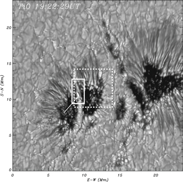
Figure 1. Part of TiO white light image (705.7 nm), observed by BFI/GST at 19:22:29 UT. The white arrow indicates brightness enhancement that occurred above an OCC inside the LB. The solid line box, corresponding to a MFE event, shares the same FOV with Figure 5. The dash line box marks the FOV of Figure 6.
Download figure:
Standard image High-resolution imageThe photospheric data were collected using a 1 nm interference filter centered at the head of the TiO 705.7 nm band with a FOV 70'' × 70'' at 0 034 pixel−1 image scale. The data were taken as bursts of 70 images with the exposure time for each frame of 0.18 ms. Figure 1 presents a part of 19:22:29 UT TiO image, showing the observed AR.
VIS is based on a single Fabry–Pérot etalon to produce a narrow bandpass (0.007 nm) over a 74'' × 68'' circular FOV at 0029 pixel−1 image scale, tunable from 550 to 700 nm. The temporal cadence of VIS instrument when observed at a fixed wavelength is about 2 s. There are 13 preset wavelength positions with the possibility to choose an arbitrary number of positions during observations. Typically, a burst of 25 frames are taken for each wavelength position with the exposure time varying from 7 to 25 ms when moving from line wings to line center. The cycle cadence depends on the number of scanning wavelengths and the size of the burst and may range from 3 to 30 s. In this study, the VIS spectroscopy observations were performed at Hα line center, ±0.04, and ±0.08 nm. The total temporal cadence for BFI and VIS were set before 19:01 UT to 30 and 40 s accordingly, then the cadence was decreased to 15 and 25 s as seeing conditions improve.
NIRIS uses a dual Fabry–Pérot etalon that provide an 85'' round FOV imaged on a Teledyne camera, which is a 2k × 2k HgCdTe closed-cycle Helium cooled IR array. A dual-beam system simultaneously captures two polarization states side by side, each 1024 × 1024 pixels in size, resulting in an image scale of 0083 pixel−1. The primary spectral lines used by NIRIS are the Fe i 1564.85 nm and the He i 1083 nm red component. The Fe i bandpass is 0.01 nm while the He i bandpass is 0.005 nm. Polarimetry measurements are performed using a rotating 0.35λ wave plate that allows us to sample 16 phase angles at each of more than 60 line positions (40 for the Fe i 1564.8 nm) with a cadence of 126 s to perform one full spectropolarimetric measurement including the full-Stokes I, Q, U, V. The Stokes data polarization calibration and inversion procedures are described in Ahn & Cao (2019). Sixteen modulated images are taken at each line position and the exposure time for each frame is 33 ms. Selected Stokes profiles are shown in Figure 2.
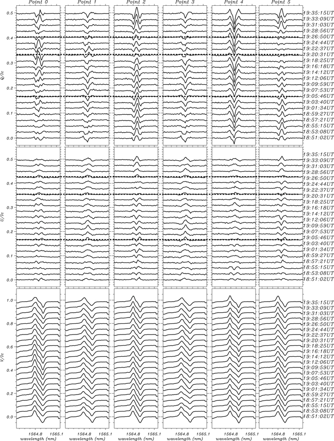
Figure 2. Normalized Stokes Q/U/V profiles at each point mentioned in Figure 3 during the MFE. Dot lines in top panels (Stokes Q) and middle panels (Stokes U) mark the time when the emerging transverse magnetic field structure appeared, peaked and destructed.
Download figure:
Standard image High-resolution image3. Data Reduction and Analysis
The AR was observed from 17:55:20 UT to 22:57:42 UT, while the data between 18:51:02 UT and 19:35:15 UT were selected for this study. Data sets of different wavelengths were spatially co-aligned for the time of 2016.02.09 18:51 UT by taking HMI/SDO continuum image as reference.
The GST photospheric TiO and chromospheric Hα data were flat fielded and then speckle reconstructed using the Kiepenheuer-Institute Speckle Interferometry Package code (Wöger et al. 2008). Additionally, the Hα data set was processed with two-dimensional discrete wavelet transform (DWT; Akansu et al. 1990) and principal component analysis (PCA; Pearson 1901) reconstruction methods to remove noise patterns in the reconstructed Hα images. The utilized technique works as follows. First, an image is decomposed by fourth-order Daubechies wavelet (Daubechies 1992) with four levels and an approximation is generated, as well as horizontal and diagonal coefficients for each level. Second, we applied PCA reconstruction technique to the horizontal and vertical coefficients at each level to extract the horizontal and vertical pattern of coefficients in the wavelet domain. Next, we recomposed the extracted coefficients by an inverse DWT and generated image with horizontal and vertical noise pattern in a spatial domain. Finally, we removed the noise patterns from the observed image.
We applied two inversion methods to the NIRIS Stokes profiles. The Milne-Eddington (ME) inversion code used in our study was developed by J. Chae, and its early version was applied to the Hinode/SP data (Chae & Park 2009). An inverted data set includes nine parameters among which are the total magnetic field flux density, the inclination, and azimuth angles, and the Doppler shift. This code uses a simplified model of solar atmosphere and performs very fast inversion, which is desirable when inverting a large data set. We applied it here to a series of spectropolarimetric line profiles to analyze the temporal evolution of the MFE event. To better understand the height dependence of the magnetic field and to obtain reliable thermal information, a more complex inversion should be used. For this purpose, we applied a Stokes inversion method based on response functions (SIR) developed by Cobo & del Toro Iniesta (1992). A simple SIR inversion model with one-component (1C) gradient magnetic field configuration—three nodes for perturbing temperature, linearly evolving magnetic strength, line of sight (LOS) velocity, inclination, azimuth, and no straylight correction applied—works well for the umbra, the LB, and the most part of the penumbra in this region. The inversion results contain data for different solar atmosphere heights ranging from Log τ = 1.4 to Log τ = −4. A comparison of the inversion result between the two methods are presented in Figure 3. We resolved the 180° ambiguity by using HMI/SDO ambiguity-resolved vector magnetic field as reference and applying the acute angle approach, i.e., azimuth was assigned in the direction that was making smallest angle with the corresponding HMI azimuth.
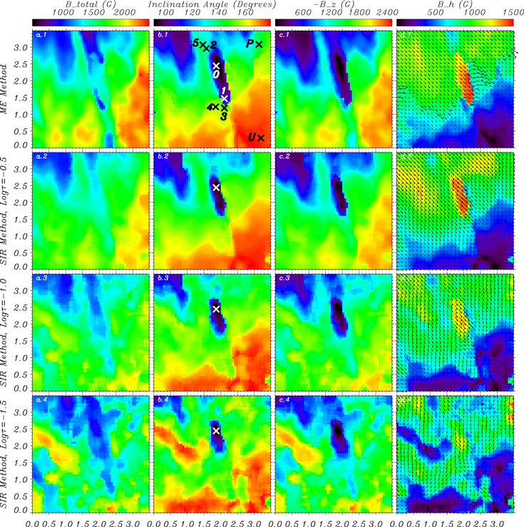
Figure 3. Comparison of different Stokes inversion methods applied to the NIRIS 19:20:31 UT Stokes profiles. The first row is the inversion results from ME method and the others are from SIR method (Log τ = −0.5/−1.0/−1.5 or τ = 0.316/0.1/0.0316). Column a shows total magnetic field and the images in columns b, c, and d represent the magnetic inclination angle, vertical and horizontal magnetic flux density in the heliographic coordinates, respectively. The four images in each column are drawn with the same dynamic range. Point 0 with white cross symbol in b.1 marks the only pixel that contains the opposite polarity in the ME inversion. Point U and P with black cross symbol represent selected umbral and penumbral pixel. The magnetic field orientation vectors (black arrows) in the horizontal plane are overplotted on column d images.
Download figure:
Standard image High-resolution imageAfter inspecting the SIR inversion results at several selected pixels, we found that the 1C magnetic field model did not satisfactorily fit the observed profiles in the flux emergence region. Some of the fitting samples are provided in Figure 4. The last column of Figure 4 shows that 1C inversions work well for the brightening at the LB OCC region (point 4) and only one strong vertical magnetic field component may be used to invert the data at this pixel. The left column displays the observed Stokes profiles and the 1C inversions at point 0. The thing to notice is that the lobes in the observed Q profile are closer together than those in the V profile and they have smaller width. As for the 1C inversions, the lobes in the inverted Q profile are simply too broad to fit the observed ones, but they match the width of Stokes V lobes. The reason why the 1C inversions failed to match the observations is that at this pixel we probably have a mix of two magnetic components. The one that is more horizontal and produces the Stokes Q signal has a lower field strength, while most of the contribution into the Stokes V comes from a more vertical component This is why the lobes in Q have a lower width, while Stokes V lobes are more separated.

Figure 4. Examples of Stokes line profile fitting results of SIR inversions. The black solid line in each panel represents for observation profile. The red and blue dash line in each panel shows the fitting result. Left column: the one-component fitting for the point 0 in Figure 3, with the location of the lobes in Stokes Q and V marked by black and red dot lines. Second column: the two-component fitting result for the Point 0. Right two columns are the fitting results for point 3 and point 4 in the Figure 5. The one-component fitting works well for point 4, while the two-component fitting is required for point 3.
Download figure:
Standard image High-resolution imageWith an ultrastrong gradient (nodes for B/gamma/phi ≥2), we can emulate those two different components in one stratification; however, the fields have to change their inclination by about 90° within the range Log τ 0 to −2, and their fields flux density also has to change rapidly within that narrow spatial range. In this case, a two-component (2C) magnetic field model is needed for those pixels that display this kind of Stokes profiles (Figure 4, second column).
We then applied a 2C inversion atmospheric model to selected pixels of interest, and assigned two nodes for temperature with a constant magnetic field and LOS velocity,. For point 0, the 2C inversion resolved a slightly inclined strong vertical magnetic field component (which dominates the penumbra region) and a weak horizontal magnetic field component (which is common in the flux emergence region). Similarly, for point 3, located at the magnetic minimum region, we found an opposite polarity magnetic field component that is mixed with the background penumbra magnetic field.
The 1C and 2C inverted and deprojected magnetic flux density and inclination angles for the selected pixels are listed in Table 1.
Table 1. Inverted Magnetic Field Magnetic Flux Density and Inclination with SIR Method
| Point | 1C or 2C | Btotal (G) | γ (°) |
|---|---|---|---|
| U | 1C | 2150 | 176 |
| P | 1C | 1617 | 147 |
| 0 | 2C | 1549 | 158 |
| 1042 | 69 | ||
| 2 | 2C | 1634 | 155 |
| 849 | 112 | ||
| 3 | 2C | 1458 | 147 |
| 857 | 53 | ||
| 4 | 1C | 1740 | 156 |
Download table as: ASCIITypeset image
4. Result
4.1. Temporal Evolution of the MFE
Figure 1 presents a photospheric image of the MFE event observed in the AR NOAA 12494. A significant brightness enhancement occurred at the top of the LB OCC. A regular granular structure of the LB was replaced by one elongated OCC, with one endpoint moving along the LB toward the sunspot center (inner endpoint, white arrow) and the other one radially outward (outer endpoint). In the area marked by a dashed line, a plasma ejection event was triggered and a brightening at its footpoint was observed in the Hα image between the LB OCC and one of the sunspot umbrae.
Figure 5 shows the temporal evolution of the flux emergence event as seen in various wavelengths. Each panel displays the same FOV outlined by the solid line in Figure 1 (see the online animation with a larger FOV). The panels in the upper row present photospheric TiO images. As the OCC (marked with the white line) expanded to reach approximately 2 Mm in length, two enhanced intensity TiO patches developed near the endpoints of the expanding OCC (black contours in the image of 19:22:37 UT). The green contours, obtained by creating running difference images, represent 25% brightness enhancement relative to the running background obtained by averaging five consecutive TiO images acquired during a 75 s interval prior to 19:21:44 UT. The TiO brightenings first appeared at 19:21:44 UT and remained noticeable until 19:27:14 UT. The difference between the 19:22:29 UT image and the background showed a significant central brightness enhancement and a noticeable brightening at lower right. An inspection of unprocessed raw TiO images confirmed them to be real enhancements and not intensity fluctuations introduced by data reconstruction.
Figure 5. Overview of GST data set. The panels present, from top to bottom 2D maps, evolution of TiO Photosphere, total linear polarization, LOS Doppler velocity, and Hα off-band, transversal and longitudinal magnetic field flux density. The enhanced LB brightening that first appeared at 19:21:44 UT is confirmed by creating differential images. Green contours presented in the TiO image at 19:22:37 UT represent 25% brightness enhancement to the running background. The black contour indicates 1.3 times of the average intensity of the granulations in the nearby quiet Sun region. Another minor brightening located at the edge of the LB (cospatial to the green contour in the lower right) was in the same position of the Hα jet footpoint. The white lines indicate the axis of the emerged flux. The flux emergence lasted from 18:53 UT until 19:26 UT and the flux density of transverse magnetic field peaked at 19:20:31 UT. The online animation illustrates the temporal evolution. Numbers and "X" symbols mark five points for which magnetic flux time profiles and Stokes parameters will be analyzed (maximum inclination (0), Doppler endpoints (1 and 2), transverse field minimum (3), and TiO brightenings (4 and 5).
(An animation of this figure is available.)
Download figure:
Video Standard image High-resolution imageMaps of the total linear polarization (L =  ) and Doppler velocity obtained from the NIRIS spectropolarimetry data are displayed in the second and third rows of Figure 5. According to the data, the emergence lasted for about 30 minutes. It began at a location that already had a lower magnetic field flux density compared with the surroundings. At 18:53 UT, NIRIS data showed no magnetic signatures of this new flux, and only a strong upflow of about 1.5 km s−1 at the site of future emergence was distinct in the data. By 19:10 UT, the upflow subsided and the transverse magnetic field showed up at the location of the original upflow. NIRIS Doppler maps showed two LOS velocity patches that have developed in association with the flux emergence. The inner endpoint was associated with a compact (<03) downflow with velocities exceeding 1.5 km s−1 at their peak time (19:20 UT), while the outer endpoint only showed very weak downflows that turned into equally weak upflows (approx. 0.1 km s−1) by 19:20 UT.
At the same time, the LOS magnetic field began to gradually increase at the inner endpoint, while the LOS field at the outer endpoint remained much lower. By 19:20 UT, the transverse flux has peaked, while the LOS field showed strong asymmetry at both endpoints. However, no opposite polarity features were detected at that time, or any other time during the emergence. Compared to the pre-emergence state, the LOS magnetic flux density at the inner (umbra) endpoint has increased from approx 500 G level to over 1000 G, while at the outer endpoint the increase was much smaller and the resulting field did not exceed 900 G level.
Figure 6 displays off-band Hα −0.08 nm images, in the same time series as of Figure 5, showing a portion of a small sunspot with two umbral cores separated by a thin LB seen in these panels along their left edge. At approximately 19:17 UT, a compact chromospheric brightening developed at the very edge of the umbra next to the LB (outlined by the white box). Before the brightening onset, several nearly collimated jets were ejected in the direction of the umbra (white arrow) from that compact location forming a narrow fan-line structure. The tips of the jets were aligned and moved together forming a well-defined front. The jets did not exhibit any translational or swaying side-ward motions and increase of their apparent length was the only distinct evolutionary parameter.
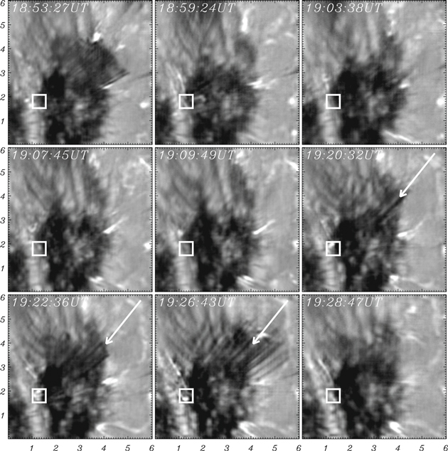
Figure 6. Chromospheric jetting activities observed with off-band Hα −0.08 nm. Time sequence of the displayed images is same to Figure 5. FOV of each panel is indicated by the white dashed line box in Figure 1. A band of narrow straight jets (white arrow) rooted at a compact brightening (white box, indicating the same area of the blue box in Figure 5), located at the edge of the LB and the sunspot umbra. The brightening first appeared at 19:17 UT and disappeared at 19:26 UT and was associated with the jet during the entire existence.
Download figure:
Standard image High-resolution imageIn Figure 7, we plot orientations of the transverse field along the spine of the emerging structure. The orientation of the transverse field changed during the emergence process. A small differential angle between the transverse field and the longer axis of the magnetic structure (white line) was observed until the maximum of the loop structure and the differential angle has decreased after that time, so that the transverse fields became nearly parallel with the longer axis of the emerging field. We emphasize that the NIRIS magnetic field data were not resolved for 180° ambiguity here, so we use the term "orientation angle" rather than the "field azimuth." The Bx–By plots (left panel) show that the transverse field began to gradually rotate in the CCW direction at about 19:07 UT and the emerging structure can be seen between pixels 9 and 23 as a series of vertically oriented line segments. As emergence proceeded the transverse structure expanded toward the umbra. It is interesting to note that at the onset of the emergence the fields in front of the moving inner endpoint (i.e., between pixels 1–7 at 19:07 UT) appear to change their orientation from nearly parallel to the longer axis to nearly orthogonal. It can be speculated that these sudden changes may have resulted from the snow-plow effect where the emerging field was intruding into the LB compressing and folding pre-existing magnetic structures ahead of it. The field inclination has not changed drastically during the event although at the time when the emergent flux reached its maximal length. After the peak of the event the transverse field continued to rotate in the CCW direction so that the differential angle changed its sign. The right panel in Figure 7 shows time profiles of the differential angle at pixels 2, 7, 12, 17, and 22. Pixel 2 is cospatial with the inner (umbral side) endpoint of the structure and the differential angle rapidly decreased as new fields appeared at that location. Pixels 12, 17, and 22 were situated near the midsection of the emerging fields and the corresponding profiles show gradual change of differential angle from 50° to nearly −50°.

Figure 7. Plot of NIRIS data slice along the white line on the emerging structure. A total of 23 pixels are selected along the white line starting from the inner endpoint (pixel 1, umbral side) to the outer endpoint (pixel 23, penumbral side). Left: transverse field evolution. Right: differential angle (difference between the direction of the white line and the azimuth angle of pixels along the white line) profiles plotted for pixels 2 (red), 7 (yellow), 12 (green), 17 (light blue), and 22 (blue). The black dashed line in each panel marks the peak time of the MFE.
Download figure:
Standard image High-resolution imageAlthough the NIRIS data did not reveal any significant features of opposite polarity associated with the emergence, the magnetic field time profiles (Figure 8) suggest a bipolar flux emergence process. During the emergence, the magnetic field became enhanced at the inner endpoint and weakened at the outer magnetic endpoint, which may indicate the emergence of a bipolar structure with a negative (sunspot) polarity at the inner endpoint and a positive polarity at the outer (penumbral side) endpoint. Both outer and inner TiO brightenings occurred during the magnetic field enhancement phase and are located close to the high magnetic gradient region. We speculate that the endpoints of the emerging structure displaced granulation ahead of them, which may lead to increased apparent brightness due to plasma compression. We would like to further note that the observed sequence of events and the rotation of the transverse fields are consistent with the emergence of a horizontal current carrying loop with a positive (negative) field endpoint located in the penumbra(umbra) of the sunspot and right handed twist.

Figure 8. Time profiles of magnetic field flux density. X-axis starts at 18:53:08 UT, when a strong blueshift first appeared at the region. Three vertical dotted–dashed lines mark the time of first appearance of the transverse field structure (19:09:59 UT), its peak time (19:20:31 UT), and the disappearance time (19:26:50 UT). Left: time Profiles of the total magnetic field flux density at point 0 (purple), 1 (blue), 2 (red), and 3 (green). Right: the same but for point 4 (blue) and 5 (red), as well the profile of the transverse magnetic flux density averaged along the white line (green). The TiO LB OCC brightening started at 19:21:44 UT and ended at 19:27:14 UT and those times are marked with the short vertical bars.
Download figure:
Standard image High-resolution image
Finally, we inspected the relevant NIRIS Stokes profiles to the selected point 0–5 (Figure 2). The Stokes V profiles were stable during the emergence and did not show any significant variations. (Figure 2, bottom panels). The most prominent variations were observed in Stokes Q profiles (upper panels) at points 0, 1, and 2 (Doppler upflows and downflows) during the emergence (between the dashed lines), which matches well with the changes in the orientation of the transverse field at those endpoints. We therefore conclude that the absence of the opposite polarity is not a consequence of failing data inversion but is rather an observational fact.
4.2. Height Dependence of the MFE
Figure 3 compares ME and SIR inversion results. Images in column c represent the vertical magnetic field flux density and column d shows the horizontal field flux density with magnetic field azimuth overplotted with black arrows. The emerging magnetic flux is prominent in the FOV. Generally, the total magnetic flux density (column a) decreases with height, which is more pronounced in the sunspot penumbral and flux emergence regions. After resolving 180° ambiguity, we converted the vector magnetic field from the native coordinate system into the heliographic coordinate system where the Bz component is normal to the solar surface. The corresponding field inclination maps are displayed in column b. The emerging flux region thus appears to have mostly horizontal fields with the inclination angle slightly above 90°, and a minor increase with height is also visible here as well as in the nearby penumbra. The inverted total magnetic field strength and inclination angle from the ME method is slightly larger than the result from the SIR method, while the presented distribution are similar. The ME result mostly corresponds around the optical depth of log τ = −0.7 of the SIR result, which supports the study of Solana et al. (2005) that Fe i 1564.85 nm line is formed slightly deeper than the Fe i 630.25 nm line. We carefully examined the inclination angle of the ME inversion result and at each height of the SIR inversion, and found only one pixel in the ME output (b.1, point 0 marked with white cross) that showed 89 8 inclination angle. Taking into account the error of measurements and inversion, that inclination angle cannot be considered as evidence of an opposite polarity field.
5. Summary and Discussion
In this study we report high-resolution observations of a MFE event in a granular LB, which was associated with enhanced brightening of the LB granules and Hα jets in the vicinity of the emerging flux. This kind of an MFE event occurring at the edge of LB is not rare, and we observed a similar event appearing twice at the same location. Photospheric expanding OCC and brightness enhancements associated with a new emerging flux have been reported before (Cheung et al. 2008; Lim et al. 2011; Yurchyshyn et al. 2013). Ji et al. (2012) and Zeng et al. (2013) also reported the granulation evolution and plasma ejections triggered by finescale MFE in the quiet Sun. However, these studies were mainly associated with bright points in intergranular lanes. Bai et al. (2019) reported similar jetting activity visible in solar chromosphere, TR, and lower corona, triggered by an emergent magnetic flux at one end of the LB structures. An elongated bright ribbon was observed at the footpoint of Hα jets along with an expanding OCC. Although lacking data on the evolution of vector magnetic field, the OCCs observed in Bai et al. (2019), could be considered as evidence of a new emerging flux (Schlichenmaier et al. 2010), which is supported by our study based on magnetic field data. The emerged magnetic structure in our study reached about 1.5 Mm in length and 0.3 Mm in width at the peak of development, and it had a lifetime of about 17 minutes, which is longer than those occurring in the quiet Sun. The total emergent magnetic flux during the emergence was about 1.91 × 10¹⁸ Mx, which is of the same order of magnitude as the total emergent magnetic flux of an MFE event observed in a quiet Sun region by Fischer et al. (2019) and it is one order larger than those reported by Jin et al. (2008), González & Rubio (2009), Gömöry et al. (2010). NIRIS Doppler data showed enhanced upflows several minutes prior the first magnetic signatures of the emerging flux. The maximum of the upflow speed is about 2 km s−1, which is at a higher end of peak upflow speeds found for quiet Sun MFE events (average speeds 0.83 km s−1 and maximum at 3–3.3 km s−1, Jin et al. 2008; Oba et al. 2017). Louis et al. (2015) also reported an emergence of a new magnetic flux near one end of an LB. The emerged dipole measured about 3 Mm along its axis, which is nearly twice the size of our event. It also showed associated Doppler speeds to be about 2 km s−1, which is very close to the speeds detected here, despite the fact that the formation height of Fe i 630.2 nm line is slightly higher than the Fe i 1564.85 nm line used in our study.
This work is the first report of brightness enhancement that occurred on the top of LB OCCs. During the emergence, the existing granulation was modified by the endpoints of the expanding OCC. Being pushed aside and compressed, the top of the granules appeared to have enhanced brightness. This MFE event was associated with jetting activity and a compact chromospheric brightening observed in the Hα line. Based on the SIR 2C inversion analysis, we speculate that the jet, located next to the bright LB OCC and magnetic field emergence inner endpoint, was triggered by magnetic reconnection between the pre-existing background umbral magnetic fields and the emerging horizontal magnetic fields. This fan-like jet system was located in the umbra in close proximity to the edge of the LB and seemed to be cospatial with the chromospheric brightening. During their evolution the jets slightly changed their orientation although they did not exhibit any significant lateral movements.
The recent work of Tian et al. (2018) classified the surge-like activities above LBs into two types. Type-I surges are characterized by constant vertical oscillating motions with a relatively stable recurrence period and they are likely to be driven by shocks that form when p-mode or slow-mode magnetoacoustic waves are generated by convective motions propagating upward to the chromosphere. Type-II surges are characterized by impulsive ejection of chromospheric material from selected locations along LBs to heights normally exceeding 4 Mm and often reaching 10 Mm or more. They are driven by reconnection between newly emerged magnetic structures in the LBs and the surrounding umbral magnetic fields (e.g., Kurokawa 1988; Tiwari et al. 2016). Bharti et al. (2017) reported λ-shaped jets in a sunspot and interpreted them as being a result of reconnection between an emerging arcade along the penumbral intrusion and the pre-existing background umbral magnetic field. The authors also noticed that instead of an arcade, rising heavily twisted flux rope (and possibly rotating) could also be the cause of the jets. Singh et al. (2012) found systematic motions of λ-shaped jets due to the emergence of a three-dimensional twisted flux rope. However, previous studies lacked support from high-resolution vector magnetic field data. Without such high-resolution data, the magnetic morphology was derived from lower resolution visible or EUV observations.
The data presented in this study is a step forward in the understanding of flux emergence and reconnection in a LB. First, we found that emerging fields seem to affect nearby LB granulation manifested as enhanced brightness of the top of a granule and prominent changes in the magnetic environment in the lower photosphere. The new flux emerging in LBs appears as a well organized, coherent, and possibly current carrying structure as evidenced by the rotation of the transverse field during the emergence. Although the event displayed signatures of a bipolar flux emergence, we did not convincingly detect any opposite polarity fields in the emergence region. One reason for that could be a specific morphology of the emerging flux. The target sunspot was located at S12, W56 so that strong projection effect combined with strongly inclined fields made it difficult to resolve the opposite polarity in the local solar surface coordinate system. At that longitude, a significant fraction of the vertical field will be observed as transverse fields so that ambiguity resolution and correction for the projection effect are necessary to reveal real morphology of the emerging flux. Additionally, the outer penumbral endpoint that is supposed to be of the following polarity could have lower field intensity, which probably presented additional difficulties for resolving and detecting these magnetic elements at that viewing angle.
BBSO operation is supported by New Jersey Institute of Technology and US NSF AGS-1821294 grant. GST operation is partly supported by the Korea Astronomy and Space Science Institute, the Seoul National University, the KLSA-CAS and the Operation, Maintenance and Upgrading Fund of CAS for Astronomical Telescope and Facility Instruments. X.Y. was supported by NSF grants AGS 1821294, 1614457, and National Science Foundation of China (NSFC) 11729301. V.Y. acknowledges support from AFOSR FA9550-15-1-0322 and NSF AST 1614457. The authors thank BBSO staff for data acquisition, and Dr. Kaifan Ji for Hα data image reconstruction. Authors also thank Dr. Haisheng Ji for multiple wavelength data analysis, and Mr. Jiasheng Wang for resolving 180° ambiguity of magnetic azimuth. X.Y. is thankful to the High Altitude Observatory (National Center for Atmospheric Research) for organizing the School on Spectropolarimetry & Diagnostic Techniques and training the young scientists with Stokes inversion methods. X.Y. is greatly thankful to Dr. Christian Beck for the detailed instructions to the 1C and 2C SIR inversion methods.