


Abstract
We have performed a spectroscopic observation over the south polar coronal hole (PCH) with the Hinode Extreme-ultraviolet (EUV) Imaging Spectrometer (EIS) during an on-orbit partial solar eclipse. In this partial eclipse, the Moon passed through the EIS observing area that was set in the south PCH at the height of 0.9–1.4 solar radii. Using the lunar occultation, we have corrected for the scattered light contamination from bright regions of the Sun that is present in the dark PCH emission line profiles. The nonthermal width of the corrected emission line profile in the PCH increases from the limb toward the high-altitude corona. It has also been confirmed that the nonthermal width tends to decrease beyond ∼1.2 solar radii. These results are consistent with the model in which outward-propagating Alfvén waves start being dissipated at ∼1.2 solar radii, as previously reported. The reduced energy within ∼1.4 solar radii contributes to atmospheric heating and the initial acceleration for the solar wind in the low corona. The remaining energy flux at 1.4 solar radii may be dissipated in the distant corona and is sufficient to provide the additional acceleration required to drive the fast solar wind.
Export citation and abstract BibTeX RIS
1. Introduction
The fast solar wind, with velocities of 700–800 km s−1, is known to originate from coronal holes (Krieger et al. 1973; McComas et al. 1998). These coronal holes are the darkest coronal regions on the Sun and are commonly found in polar regions (polar coronal holes; PCHs). The speed of the fast solar wind cannot be explained by the thermally driven mechanism proposed by Parker (1958, 1963) alone, because the source was found to be coronal holes with a low coronal temperature of ∼1 MK (Habbal et al. 1993 and the references therein). The mechanism producing the fast wind has been investigated to understand further acceleration and simultaneous heating of the fast wind plasmas.
The most promising mechanisms for producing the high-speed stream are associated with Alfvén waves, whose remnants have been found in interplanetary observations (Coleman 1967; Belcher & Davis 1971). Among many modeling studies (see references in Hollweg 1990 and Cranmer et al. 2017), recent time-dependent MHD models have shown that the transverse motion of the magnetic flux tube on the photosphere can excite Alfvén waves that accelerate the fast solar wind (Suzuki & Inutsuka 2005; Matsumoto & Suzuki 2014; Shoda et al. 2018). The height dependence of energy dissipation to be compared with observations is shown in Matsumoto & Suzuki (2014). High-speed jet structures have been found at the base of coronal holes (Brueckner & Bartoe 1983; Cirtain et al. 2007; Sako et al. 2013) and recent white-light observations show that the mass flow by such jets reaches the height beyond 2 solar radii (Hanaoka et al. 2018). Although this is a mechanism to accelerate the coronal plasmas to the distance beyond 2 solar radii, it is not the primary mechanism for acceleration of the fast solar wind, because the mass flux is not sufficient to explain the whole fast winds.
The presence of Alfvénic waves has clearly been detected by high-resolution imaging observations with the Solar Optical Telescope (SOT; Tsuneta et al. 2008a; Suematsu et al. 2008b) on Hinode (Kosugi et al. 2007) in solar prominences (Okamoto et al. 2007) and in spicular structures (De Pontieu et al. 2007; Suematsu 2008a; Okamoto & De Pontieu 2011) and with the Hinode X-ray Telescope (XRT; Golub et al. 2007) in X-ray jets (Cirtain et al. 2007). Similar motions have been found in the coronal imaging observations (Tomczyk et al. 2007; McIntosh et al. 2011). In the present study, we have investigated characteristic plasma motions of Alfvénic waves in a PCH based on a spectroscopic observation using the Hinode Extreme-ultraviolet (EUV) Imaging Spectrometer (EIS) (Culhane et al. 2007).
Emission lines observed in the solar transition region and corona are broadened not only due to thermal motions of the emitting ions, but also due to nonthermal motions, such as Alfvén waves (Mariska 1992). The excess broadening by excess collective ion motions in the hot plasmas is called nonthermal broadening or nonthermal velocity in the unit of velocity. The nonthermal velocity is likely caused by the velocity fluctuations associated with Alfvén waves. Previous studies have shown that the energy flux estimated from the nonthermal velocity is sufficient for heating the corona and accelerating the fast solar wind (Withbroe 1988). The nonthermal velocity increases with distance from the coronal base toward the higher altitude (Hassler et al. 1990). A relation between the nonthermal velocity and electron density in the corona, which expresses the energy transfer of Alfvén waves without energy dissipation, has been reported from SUMER and EIS observations (Banerjee et al. 1998, 2009). A signature of wave damping in the inner corona has been shown in Doyle et al. (1999) and Hahn & Savin (2013) near 1.2 solar radii, above which the nonthermal velocity decreases.
The emission line profiles in dark coronal regions may be affected by light from bright areas due to light scattering within the instrument. Dolla & Solomon (2008) have argued that the decrease of the nonthermal velocity starting at 1.1–1.2 solar radii in SUMER observations is not real, but rather is a systematic effect caused by the instrumental stray light signals from bright components of the solar disk. The stray light that they have defined is caused by the enhanced wing component of the point-spread function of the instrument due to a scattering process on the optical surface. The diffraction from the supporting mesh at the EIS entrance filter also causes light from bright regions to appear in the dark target regions, but the point-spread function scattering dominates the diffraction effect because the effects of diffraction are amplified only at specific distances from the source. For the purpose of improved measurement, Hahn & Savin (2013) have estimated the scattered light component in their analysis with EIS by a model that is made from the data with a Hinode on-orbit eclipse of a different date than their observation. The emission line profile to be subtracted from the target region for the correction of scattered light signals cannot be estimated from the model in Hahn & Savin (2013), because the line intensities of all the points in the instrument field of view (FOV) contribute to the components to be subtracted with different weights. The line profile in the corona at 1.2–1.4 solar radii is highly uncertain.
We carried out a spectroscopic observation of a coronal hole above the southern polar region with the Hinode EIS during a partial solar eclipse that occurred in a satellite orbit of Hinode on 2017 August 21, which was the date of the total solar eclipse across the United States. In this paper, we show the height variation of nonthermal velocity in a coronal emission line over the height range of 1.0–1.4 solar radii by correcting the contribution of scattered light photons of instrumental origin through measurements of the line profile during the occultation of the corona by the Moon's passage on the instrument FOV. Our firm measurement fundamentally supports the essential conclusion of Hahn & Savin (2013), but our scattered light correction is based on a direct measurement whereas theirs is based on a model and may be insufficient. We also show our views from the results in the present study.
2. Observations
For safe spacecraft operation, the operation team of the Hinode satellite has been watching opportunities of the on-orbit solar eclipse to predict the irradiance to the solar array paddles that produce the electrical power of the spacecraft. The Moon trajectory for each eclipse opportunity has been predicted by Dr Soma of the National Astronomical Observatory of Japan. Using the same eclipse opportunity, we have planned the measurement of the coronal emission line profile in a PCH with the Hinode EIS.
The scattered light of instrumental origin can be estimated while the Moon completely covers the target region. For a period of 19:30–20:01 UT on 2017 August 21, we have run an EIS observing program with  wide slit in the raster scan mode of
  (EW × NS) FOV and of
  raster steps. The exposure duration at each raster point was 60 s. The spacecraft was pointed to the position near the south pole of the Sun, and the EIS slit was set along the radial direction of the Sun to cover the polar coronal region of 0.90–1.43 solar radii. For the confirmation of the position of the Moon during the partial eclipse, we also observed the X-ray Sun with the Hinode XRT every 30 s.
The EIS observing program has 25 spectral windows, and we only use Fe xii lines at 186.86 and 195.12 Å (hereafter Fe xii 186 and Fe xii 195) in this study. In particular, the brightest Fe xii 195 line has enough emissivity for plasmas at temperature of ∼1.2 MK, which Doyle et al. (1999) have reported above a PCH based upon the radial electron density structure derived from a Si viii line intensity ratio, and is one of the suitable EUV lines for the line-profile analysis of the corona above the south PCH at a distance up to 1.4 solar radii. The other emission lines are so dark that we cannot use those lines for this study. Since the range of electron temperature forming Fe xii overlaps with that of Fe xi that Hahn & Savin (2013) used and (Si viii) that Doyle et al. (1999) used, the same component could safely be observed in Fe xii. The disadvantage of Fe xii observations is a higher sensitivity to the foreground and background quiet-Sun corona. On the other hand, it has an advantage at the most distant corona of 1.4 solar radii in our observations, because the most abundant Fe ionization state observed by the Ulysses/SWICS in situ measurement of fast wind plasmas that originate from a PCH is Fe xii or Fe xi (Galvin et al. 1995), and because the "freeze-in" distance (Hundhausen et al. 1968) of Fe xi where the Fe xi charge state ceases to change may recently be found at 1.5 solar radii, which has empirically been determined from a total eclipse observation (Boe et al. 2018).
Figures 1(a)–(f) show the X-ray images in a negative grayscale during the Hinode on-orbit eclipse. The shadow of the Moon is seen in each panel and moved rapidly in the XRT FOV. The rectangular box near the center of each panel indicates the EIS FOV in the raster scan. The coalignment between the XRT and EIS data is performed with coronal bright points that are identified in the reconstructed EIS raster scan image. The Moon completely covered the EIS FOV at 19:44 UT (Figure 1(c)) and also occulted one of the solar active regions on the disk. The occultation of the active region was finished slightly before the time of Figure 1 panel (d). The contribution of the scattered light from the quiet-Sun corona appears to be minor in soft X-rays. Increased scattered light signals were recorded after the Moon passed through the active region near the disk center (see Figures 1(a)–(d)), indicating that the primary sources of the scattered X-rays to the occulted area are the active regions, and the contribution of the quiet-Sun corona appears to be secondary.
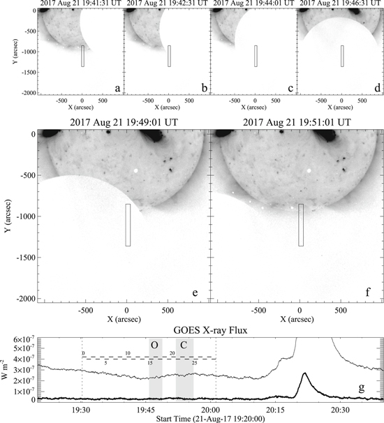
Figure 1. (a)–(f) Sequence of X-ray images recording the position of the moon during the Hinode on-orbit eclipse. Rectangular boxes indicate the FOV of the EIS raster scan observations. (g) GOES X-ray flux at the low-energy channel (1–8 Å) is shown by the solid line and at the high-energy channel (0.5–4 Å) by the thick line. The short horizontal bars indicate the exposure duration at each EIS raster position, which are labeled 0 through 29. The EIS field of view is occulted and not occulted by the Moon in the periods O and C, respectively. No remarkable flare activity is found in X-rays during the EIS observation.
Download figure:
Standard image High-resolution imageFigure 1(g) shows the X-ray flux from the entire Sun, which was measured with the X-ray flux monitor of the Geostationary Operational Environmental Satellite (GOES). We note here that we have not checked the presence of the occultation of the Sun by the Moon from the perspective of the GOES satellite. The vertical dotted lines indicate the start and end times of the EIS raster scan observation, and the 30 horizontal bars show the exposure duration at each raster position. No flare activity was identified during the EIS observation. The time range O (occulted by the Moon; 19:45:47–19:48:51 UT) indicates the period when the Moon completely covered the whole EIS raster scan area with no occultation of an active region near the disk center, while the time range C (corona above the south PCH; 19:51:58–19:56:04 UT) was the period when the Moon occulted neither the active regions nor the EIS FOV.
While we need to integrate multiple exposures to measure the line-profile shape at the distant dark corona above the limb, the number of exposures from the west-to-east raster scan that can be summed is limited by the fast passage speed of the Moon. We have spatially summed the EUV line spectra along the slit direction to raise the photon statistics. At the time of spatial summing, the data at bad pixels, those that are known to have been damaged by on-orbit radiation, were masked and not used. To further improve statistics, we have made average spectra at 10 radial sections.
The Fe xii 195 line intensity variations at two radial sections as a function of the EIS raster scan position are shown in the left panels of Figure 2. The first and fourth contacts occurred during the exposure at the EIS raster positions of 5 and 19, respectively. The time goes on with the raster position, and the EIS raster direction is from the west to the east. There are two reasons why the intensity in the EIS observing regions changed: one is the change of instrumental scattered light from the occulted corona by the Moon, and the other is the direct occultation of the EIS observing region by the Moon. The coronal section  –1.20 (
 –1.42) along the slit was covered by the Moon at the EIS raster positions 11–17 (12–18). The intensity variation during the passage is due to the change of the scattering component whose source was changing with time by the change of the occulted part of the corona according to the motion of the Moon. This is a measure of contribution of the scattering to each coronal section from various locations covered by the Moon in the southern hemisphere.
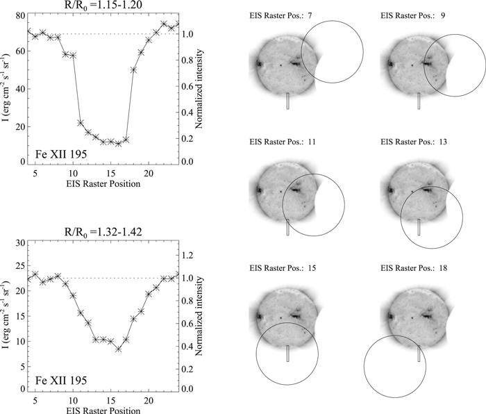
Figure 2. (Left) Integrated Fe xii 195 line intensity at each EIS raster position in the coronal sections  1.15–1.20 and 1.32–1.42. The decrease of EUV intensity due to direct occultation of the EIS FOV by Moon and reduced diffraction and scattering from the occulted disk component by the Moon are recorded. (Right) Position of the Moon outer boundaries at the central time of each EIS raster is superimposed over the AIA 193 Å band image (north is top and west is right) observed at 19:54:29 UT, which contains the shadow of the Moon near the west limb in the case of the SDO orbit.
Download figure:
Standard image High-resolution imageThe right panels illustrate the position of the Moon at the midpoint of each exposure for each EIS raster position. The Moon's position is superposed on an EUV image obtained at 19:54:29 UT that were observed in the 193 Å bandpass of the Atmospheric Imaging Assembly (AIA; Lemen et al. 2012) on the Solar Dynamic Observatory (SDO; Pesnell et al. 2012). These EUV images also contain the shadow of the Moon near the west limb, but the perspective of the eclipse observed by the SDO, which is in a geosynchronous orbit, differs from the view from Hinode. Since the AIA 193 Å band is dominated by Fe xii emission, the spatial and temporal variation of the EUV intensity recorded by AIA may be used as an indicator of the Fe xii 195 line intensity observed by EIS.
The coalignment between the XRT and AIA data has also been carried out with coronal bright points over the half disk of the Sun. Since the EIS FOV area in the AIA 193 Å images was completely free from the lunar occultation, we have checked the temporal and spatial variations of the EUV intensity in the EIS FOV from the AIA data. The spatial variation in the raster positions during the O and C periods in Figure 1(g) was within 2%. This demonstrates that there is sufficient spatial and temporal uniformity that the integration of signals across different scanning points is justified and that the comparison of signals between the periods O and C is valid. As shown in Figure 2, left panels, the intensity of the EIS target regions returned to be at the same intensity level after the Moon passage, which supports the consistency between the EIS Fe xii spectral data and the AIA 193 Å imaging data.
As described above, we have analyzed the EUV line profile of Fe xii at 195.12 Å to derive the nonthermal velocity  from the full width at half maximum (FWHM) of the observed emission line
  . The FWHM includes a contribution due to instrumental origin
  as shown in the following equation,
where  is the instrumental broadening given from the standard EIS analysis software in the Solar Software (SSW) package,
  is the Boltzmann constant, Ti is the ion kinetic temperature, Mi is the mass of ion, and W is the intrinsic line width of solar origin in FWHM. An observation with a single emission line cannot measure Ti in Equation (1) from the line width without some assumption. We assume
  for the coronal height that we investigated in the present study. It is a reasonable assumption, because the equipartition time between Fe xii ions and electrons is about 60 (600) s for solar wind plasmas of
  K and
K and  , and is a sufficiently short time for the cooling time of the plasmas.
The observed line width of Fe xii 195,  , is known to be systematically broader than that of the other Fe xii lines such as Fe xii at 193.51 Å,
  , as shown in Figure 15 in Hara et al. (2011). To account for this, a weak self-blend with Fe xii at 195.18 Å is considered to cause an excess line broadening
  . The value of
  was inferred by analyzing data from Figure 15 of Hara et al. (2011) according to the following equation.
from which we find that  23.6
23.6  or 15.3 mÅ in this study.
The density-sensitive intensity ratio of Fe xii 195.12 to Fe xii 186.86 is used to estimate the electron density. The CHIANTI spectral code version 8 (Dere et al. 1997; Del Zanna et al. 2015) was used to convert the line intensity ratio into the electron density.
In this study, we estimate the energy flux of the Alfvén wave from the emission line width by assuming that all the nonthermal velocity is due to the waves. The magnetic field strength at the coronal base in the polar region is required for that purpose, and we use the magnetic field data obtained with the specto-polarimeter (SP; Lites et al. 2013) of the Hinode SOT, the facility for Synoptic Optical Long-term Investigations of the Sun (SOLIS) at the Kitt Peak Observatory, and the Helioseismic and Magnetic Imager (HMI; Scherrer et al. 2012) on SDO. The magnetic field observation of the south pole was not executed with the Hinode SP near the eclipse time, so we use the SP data in the south pole observation on 2017 September 18 for the cross-check among different photospheric observations. The field strength at the coronal base as reference is calculated using the potential field source surface (PFSS) model (Schrijver & DeRosa 2003) in SSW.
3. Results
Figure 3 (top panels) are the average spectra at three representative coronal sections out of 10. The thick (thin) line in each top panel shows the spectrum  (
( ) as functions of wavelength λ and radial distance R during the period O (C) in Figure 1(g). The spectral difference
  , defined by
  , is a corrected spectrum at a radial distance R, which is shown in the bottom panels of Figure 3. At the most distant section (
 1.32–1.42;
  : the solar radius), the intensity level of the instrumental origin reaches ∼40% of the observed intensity.
  is made from the data at the EIS raster positions 15–17, in the periods of which the Moon covered the entire EIS FOV and the south polar region as shown in the right panel of Figure 2. Since the south polar region was covered by the Moon, the contribution of this part of the Sun to the instrumental scattered light in the EIS FOV is missing, and is not corrected in the spectral difference alone. Although we consider the contribution of the occulted south polar region later, we first ignore it for simplicity. However, the instrumental scattered light from regions outside the occulted area is totally corrected at least.

Figure 3. (Top) Average Fe xii line profile at 195.12 Å during the time ranges C (thin line) and O (thick line) at three different radial positions. (Bottom) Difference of the spectra between the thin and thick lines in the top panels.
Download figure:
Standard image High-resolution imageThe spectral difference  in Figure 3, bottom panels, is fitted by a single Gaussian function, and we have estimated the nonthermal velocity
  using Equation (1). The standard analysis routine in the SSW is used in deriving the EIS instrumental width
  . Since Fe xii 195 is broader than the nearby lines due to blend lines, we have estimated its instrumental width using Equation (2). The electron temperature
  , which is used as a measure of the Fe xii ion temperature, is assumed to be 1.0 MK here, and the assumption is sufficient for estimating the nonthermal velocity because the nonthermal velocity in Equation (1) has a weak dependence on the ion temperatures. (See Figure 14 in Hara & Ichimoto 1999 for a reference by regarding the horizontal axis as FWHM in the unit of velocity.) The assumed temperature of 1.0 MK is roughly consistent with the hydrostatic equilibrium temperature derived from the radial variation of electron density, which is shown in Figure 4. That density was determined using the density-sensitive intensity ratio of Fe xii 195 to Fe xii 186. For the density analysis, the scattered light correction used for the Fe xii 195 data has also been applied to the Fe xii 186 data. Since the electron density as a function of distance is close to that in Hahn & Savin (2013), similar plasmas in the PCH would also be observed. The electron density can only be determined up to 1.1 solar radii due to the weak Fe xii 186 signals. This may be improved by the inclusion of a white-light observation in the data analysis. The other PCH density measurement in Doyle et al. (1999) and a PCH density model in Cranmer & van Ballegooijen (2005) are also shown in Figure 4 as references.
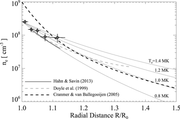
Figure 4. Electron density in PCH estimated by the Fe xii line intensity ratio  in diamond symbols. Thin solid lines give the variation of electron density for the hydrostatic cases of 0.8, 1.0, 1.2, and 1.4 MK. The thick solid line is a density structure derived from an Fe xi line intensity ratio in Hahn & Savin (2013) and the thick dashed line in gray is from a Si viii line intensity ratio in Doyle et al. (1999). The thick dashed line in black is from the model of Cranmer & van Ballegooijen (2005).
Download figure:
Standard image High-resolution imageFigure 5 shows the nonthermal velocity varying with the radial distance overplotted with the results from Figure 3 in Hahn & Savin (2013). The trend within 1.2 R0, where the signal of the instrumental origin is low, is consistent with previous studies (Banerjee et al. 1998, 2009; Doyle et al. 1999; Hahn & Savin 2013). The decrease or flattening of the nonthermal velocity at distances above ∼1.2 R0 is clearly shown. When the whole nonthermal velocity is explained by the plasma motions associated with outward-propagating Alfvén waves, and if energy is conserved so that there is no energy dissipation during the propagation, then the nonthermal velocity  is expected to vary as
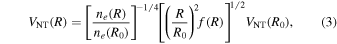
where  is electron density at radial distance R and f(R) is the area expansion factor that was introduced in Kopp & Holzer (1976) and that is usually derived from coronal structures observed in the white-light corona. The quantities
  , and σ are model parameters used to express f(R).
  was used in Munro & Jackson (1977), and
  in Cranmer et al. (1999). We have estimated the values to be
  from Figure 1 in Hanaoka et al. (2018). The trend in Equation (3) with the adopted parameters is plotted as the dashed line in Figure 5, and the dotted line in Figure 5 indicates the case of
  . Although the radial solar wind speed at 1.3–1.4 solar radii is expected to be ∼20
  , the effect of the radial speed to the line broadening is negligible (
 ) for these areal expansions.
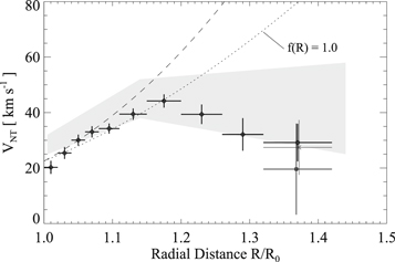
Figure 5. Nonthermal velocity  as a function of radial distance from the limb. Dotted and dashed lines indicate the nonthermal velocity for cases without energy dissipation with different radial area expansion f(R). See the text for details. The shaded area schematically shows the result in Hahn & Savin (2013). Diamond symbols are derived from the subtracted spectra whose examples are shown in Figure 3 (bottom panels). Cross symbol is from the further subtraction of scattered photons from the quiet-Sun near the EIS FOV. Square is from the measurement at raster point 18 alone.
Download figure:
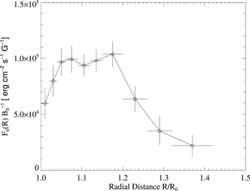
Standard image High-resolution imageSince it is difficult to see the energy flux of Alfvén waves from Figure 5, we have made a plot in Figure 6 that shows the following equation;
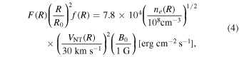
where F(R) is the wave energy flux at a distance R, and B0 is the magnetic field strength at the coronal base. The left-hand side equation that is newly defined as  indicates the wave energy flux F(R) at a distance R after correcting for the spreading out of the energy with area expansion, thereby describing the energy as a function of height in terms of an equivalent energy flux at the coronal base
  . If all the wave energy originates at the base
  , the difference
  gives the consumed energy flux below distance R. Note that the ordinate of Figure 6 is
  , which can be evaluated from observables of electron density ne and nonthermal velocity
  , and is independent of the selection of the expansion factor f(R). We have used the electron density as a function of distance, which is shown in Figure 4 by the thick solid line for
  1.0 MK, and the radial variation of the nonthermal velocity in Figure 5.
Figure 6. Remaining energy flux of Alfvén waves at a radial distance  per unit magnetic field strength at the coronal base (
 after correcting for radial expansion, so that the quantity plotted is the remaining energy flux as if it were measured at the base of the corona. Radial magnetic field strength at the coronal base of ∼4 G needs to be multiplied for evaluating the absolute energy flux.
Download figure:
Standard image High-resolution image
To obtain an absolute energy flux, the value of the vertical axis in Figure 6 needs to be multiplied by the magnetic field at the coronal base of the south polar region on 2017 August 21. The polar field strength B0 ranges from 5 to 10 G (Stenflo 1970; Tsuneta et al. 2008b; Wang 2010, 2017). The polar mean radial field near the south pole (latitude of −75° to −65°) on 2017 August 21 is −4.1 G on the photosphere from the Kitt Peak SOLIS observation. The PFSS model using the SDO HMI magnetograms gives the mean radial field of −5.9 G on the photosphere and −3.6 G at a coronal base ( ). The average radial field strength near the south pole (latitude of −90° to −80°) is about −6 G on the photosphere from the Hinode SP observation on the 2017 September 18. When we adopt the mean radial field of 4 G at the coronal base, the energy flux of Alfvén wave there is
  erg cm−2 s−1. The energy flux of
  erg cm−2 s−1 at the coronal base remains at the coronal distance of
  .
.
4. Discussion
The signals of the EIS instrumental scattered light in the corona at 1.0–1.4 solar radii have been obtained in an on-orbit eclipse in order to obtain a better estimate of the line width that contains the nonthermal width, possibly due to the outgoing Alfvén waves. The instrumental signal level from the other points on the solar disk to an observing point beyond the limb is much lower than that from the corona near the solar limb and is comparable to the real signal at 1.3–1.4 solar radii. However, the contribution of the southern polar region, which is covered by the Moon near the time of the EIS raster position 15, to the EIS FOV is not corrected in the above estimate, so that the removal of the instrumental signals may be insufficient.
A better estimate of the instrumental component in the observed signals is possible using the integrated line intensity at the radial distance of  1.32–1.42. For the EIS raster position 11 in Figure 2, the EIS FOV at that distance was not occulted by the Moon. The intensity at that raster position dropped by 27% compared to the non-eclipse condition at the raster positions 0–3. After the start of the partial eclipse at the raster position 4, the drop of intensity is negligible, implying that the scattered light signals from the quiet-Sun corona at large distances from the EIS FOV are very small. The intensity drop in the EIS FOV became remarkable when one of the active regions and the quiet-Sun corona near the EIS FOV were occulted by the Moon. The Moon at the raster position 11 almost covered half of the disk, and that condition can be used to estimate the contribution of the scattered light signals from the entire disk to the EIS FOV at the distance of
  1.32–1.42 if the scattering process is a function of distance r from the source. The AIA 193 Å images show that the Fe xii signals from the eastern part of the Sun to the EIS FOV is almost the same as that from the western part as long as the scattering is only a function of the distance r. If this is true in the EIS Fe xii 195 observation, then the signal level to be removed from the EIS observed intensity at the non-eclipse condition is almost twice the intensity drop at the raster position 11, 54% of the non-eclipse signal in the EIS FOV. The measured signal at the distance of
  1.32–1.42 is 44% of the intensity at the non-eclipse condition at the EIS raster positions 15–17, which are the periods during which the EIS FOV was completely occulted by the Moon, and is underestimated by 23% (
 ).
).
We note that this does not imply that the contribution of signal from active regions to the EIS FOV is dominant. The intensity variation from the EIS raster position 13 to 15 is small, while one of the active regions reappeared behind the Moon. This suggests that the signal from the quiet-Sun corona with a larger area is the primary contribution to the scattered light at the distance of 1.3–1.4 solar radii in the EIS FOV. This could be understood by the ratio of intensity per unit emission measure for hot active-region plasmas and that for cooler quiet-Sun plasmas. For plasmas of unit emission measure, XRT has an order of magnitude larger sensitivity for plasmas in active regions than in the quiet-Sun, while the EUV Fe xii line has a weaker contribution at the characteristic temperature of active-region corona than that of the quiet-Sun corona. This is also valid for the scattered light from the source regions. The EIS emission line measurement at the distance of 1.3–1.4 solar radii is largely contaminated by the quiet-Sun corona and the observed line profile will show the line broadening that is nearly the same as that of the quiet-Sun corona. Therefore, a line profile of the scattered light component is mandatory in order to subtract the contaminating scattered light contribution at dark observing points.
The EUV spectra from the entire quiet-Sun corona that was occulted by the Moon at the EIS raster position 15 cannot be known. If it is the same spectral shape as what EIS observed, a further subtraction of the instrumental component and the updated line width measurement are possible by considering the underestimated integrated intensity. The data point plotted with a thick gray cross at 1.32–1.42 solar radii in Figure 5 is the updated nonthermal velocity. We also add a measurement from the EIS raster position 18 at 1.32–1.42 solar radii plotted as a thin square in Figure 5. While this area was completely covered by the Moon, the quiet-Sun corona in the southern region is mostly visible outside the Moon as shown in Figure 2. The  value at this height is nearly free from the instrumental effect, and supports the other estimates at 1.32–1.42 solar radii. The fraction of scattered light signal there is
  .
.
We point out that the fraction of the scattered light level at a far distance is larger than that in Hahn & Savin (2013) and that the correction of the scattered light may be insufficient in their study. But we find that the nonthermal velocity variation as a function of coronal height is consistent with those in Doyle et al. (1999), Hahn & Savin (2013), and Banerjee et al. (2009). Since  at a far distance of 1.3–1.4 solar radii is nearly the same as those near the limb (R ∼ R0), the fraction of the scattered light signal may not affect the
  estimate as we have shown in Figure 5.
We discuss the results from the present study here in comparison with those from a numerical simulation in Matsumoto & Suzuki (2014), which explains coronal heating and solar wind acceleration in an open magnetic field region by the dissipation of Alfvén waves that are excited at the photosphere and propagate into the corona. The damping process in the low corona is mostly due to MHD shocks in Matsumoto & Suzuki (2014). This differs from their previous work that had a lower radial resolution where they had found that the heating was by MHD turbulence (Matsumoto & Suzuki 2012). The Alfvén wave energy flux in Figure 1 of Matsumoto & Suzuki (2014) gradually changes with height, which is quite different from the present study that shows a significant change near 1.2 solar radii. In this study it is also found that the remaining energy flux at 1.3–1.4 R0 is sufficient for accelerating the plasma to the fast wind speed if the magnetic field strength at the coronal base is at least 4 G as observed by polarimetric observations.
We note that the energy flux in Figure 6 appears to increase between 1.0 and 1.05 solar radii, though the error is relatively large. If this trend is true, one possible explanation is that there is additional Alfvén wave energy flux input in the low corona. A possible candidate to explain such an increase of the Alfvén wave energy flux is magnetic reconnection as Parker has suggested (Parker 1991). Since the scattered light level in the low corona is much weaker than the intrinsic coronal intensity, whether the additional flux is produced in the low corona will be verified with the EIS archived data by reducing the random noise through increasing the photon statistics. A better Moon trajectory would also give a simpler  estimate at every height in general.
5. Conclusions
We have measured the radial variation of the nonthermal velocity in a coronal emission line for a PCH with the Hinode EUV imaging spectrometer during a partial solar eclipse viewed from the perspective of the Hinode satellite. The scattered light signals in the observing region from bright regions on the disk are estimated and subtracted by signals during the lunar occultation. While the spectral signals of the instrumental origin to be removed are negligible below the distance of 1.2 solar radii, where the trend of the radial variation in  changes, the scattered light component is found to become ∼60% of the spectral signals at the distance of 1.3–1.4 solar radii during this observation. After correcting for the instrument scattered light, it is found that
  increase with distance within 1.2 R0 is consistent with the previous studies, which supports that Alfvén waves are propagating toward the higher altitude without significant energy loss. The wave energy is mostly consumed by the distance of 1.3 R0, which implies that the energy goes into atmospheric heating and initial acceleration of the solar wind. The remaining energy flux at 1.4 R0 is sufficient for the additional acceleration of the solar wind at a distance of 2–10 solar radii, which is expected by theoretical studies. We point out that there may be an increase of the wave energy flux in the low corona of 1.0–1.1 R0. This trend could be investigated in more detail with further EIS observations, because the number of photons in the area is sufficient under the negligible contribution of instrumental origin.
The author thanks the anonymous referee for helpful comments during the reviewing process. Hinode is a Japanese mission developed, launched, and operated by ISAS/JAXA, in partnership with NAOJ, NASA, and STFC (UK). Additional operational support is provided by ESA and NSC (Norway). GOES and SDO are US spacecraft. The SOLIS was operated by the Kitt Peak Observatory of the US National Solar Observatory. This work was supported by Grant-in-Aid for Scientific Research 15H05750. The data analysis was partially carried out by the Solar Data Analysis System in NAOJ.