


Abstract
The second LIGO–Virgo catalog of gravitational-wave (GW) transients has more than quadrupled the observational sample of binary black holes. We analyze this catalog using a suite of five state-of-the-art binary black hole population models covering a range of isolated and dynamical formation channels and infer branching fractions between channels as well as constraints on uncertain physical processes that impact the observational properties of mergers. Given our set of formation models, we find significant differences between the branching fractions of the underlying and detectable populations, and the diversity of detections suggests that multiple formation channels are at play. A mixture of channels is strongly preferred over any single channel dominating the detected population: an individual channel does not contribute to more than ≃70% of the observational sample of binary black holes. We calculate the preference between the natal spin assumptions and common-envelope efficiencies in our models, favoring natal spins of isolated black holes of ≲0.1 and marginally preferring common-envelope efficiencies of ≳2.0 while strongly disfavoring highly inefficient common envelopes. We show that it is essential to consider multiple channels when interpreting GW catalogs, as inference on branching fractions and physical prescriptions becomes biased when contributing formation scenarios are not considered or incorrect physical prescriptions are assumed. Although our quantitative results can be affected by uncertain assumptions in model predictions, our methodology is capable of including models with updated theoretical considerations and additional formation channels.
Export citation and abstract BibTeX RIS
1. Introduction
In less than five years the field of gravitational-wave (GW) astrophysics has evolved from speculating about the properties of compact binary coalescence events to having a substantial population primed for astrophysical inference. The recently released catalog of compact binary coalescences (GWTC-2), accumulated by the LIGO and Virgo GW detector network (Aasi et al. 2015; Acernese et al. 2015), has increased the number of confident detections reported by the LIGO Scientific and Virgo Collaboration (LVC) to 50 (Abbott et al. 2020b). As the endpoint of massive-star evolution, merging double compact objects can encode unique information about their progenitor systems, such as the types of galactic environments they were born in and their formation processes, the complex stellar evolution that persisted throughout their lives, and the physics of the supernovae that marked their deaths (Abbott et al. 2016a; Mandel & Farmer 2018; Vitale 2020). From this catalog, the rates of compact binary mergers in the local universe have been significantly constrained, features have been resolved in the binary black hole (BBH) mass spectrum, and a non-negligible fraction of systems have been found to have spins misaligned relative to the pre-merger orbital angular momentum by more than 90° (Abbott et al. 2020c).
Of the GWTC-2 observations, the vast majority (46) are confidently identified as BBH mergers (Abbott et al. 2020b). BBHs have a disparate array of proposed formation channels. The simple picture of two canonical BBH formation channels, the isolated evolution of a massive-star binary and dynamical assembly in a dense stellar environment, is now inadequate to capture the breadth of theoretical models proposed for BBH mergers. Both the isolated evolution and dynamical assembly paradigms have multiple subchannels with differing predictions for mass distributions, spin distributions, and the redshift evolution of BBH mergers, each with predicted local merger rates consistent with the empirical rate measured by the LVC of 15–40 Gpc−3 yr−1 (90% credible interval; Abbott et al. 2020c).
On the isolated evolution side, the standard channel involves a phase of unstable mass transfer following the formation of the first black hole (BH), initiating a common envelope (CE) phase that hardens the binary via drag forces (Paczyński 1976; van den Heuvel 1976; Tutukov & Yungelson 1993) and leading to BBHs that can merge in less than the Hubble time (e.g., Bethe & Brown 1998; Belczyński et al. 2002; Dominik et al. 2012; Belczynski et al. 2016; Eldridge & Stanway 2016; Stevenson et al. 2017b; Giacobbo & Mapelli 2018). However, theoretical models have shown that hardened BBH systems merging within the Hubble time can also form through late-phase stable mass transfer (van den Heuvel et al. 2017; Neijssel et al. 2019). On the other hand, if the progenitor stars are born in a very tight orbital configuration, they may proceed through a chemically homogeneous evolution, in which rapid rotation of the stars attained through tidal interaction leads to strong mixing, replenishing the core with elements for nuclear burning and never leading to significant expansion of the progenitor stars (De Mink & Mandel 2016; Mandel & De Mink 2016; Marchant et al. 2016). Extremely low-metallicity Population III stars in binary systems have also been proposed to have formed the high-mass BBH mergers observed (Madau & Rees 2001; Kinugawa et al. 2014; Inayoshi et al. 2017).
On the dynamical side, following the formation of BHs from massive stars in a dense stellar environment such as a globular cluster (GC), nuclear star cluster (NSC), or young open star cluster, these BHs' masses are segregated to the core of the cluster due to dynamical friction and create a dense subsystem dominated by BH interactions (Lightman & Shapiro 1978; Sigurdsson & Hernquist 1993). Strong gravitational encounters between BH systems act to produce hardened binaries, typically extracting orbital energy from the more massive components of the interaction by ejecting the lighter components (McMillan et al. 1991; Hut et al. 1992; Sigurdsson & Phinney 1993; Miller & Hamilton 2002; Gültekin et al. 2006; Fregeau & Rasio 2007) and leading to BBHs that can merge within the Hubble time (e.g., Portegies Zwart & McMillan 2000; O'Leary et al. 2006; Downing et al. 2010; Samsing et al. 2014; Ziosi et al. 2014; Rodriguez et al. 2015, 2016a; Antonini & Rasio 2016; Askar et al. 2017; Banerjee 2017; Samsing & Ramirez-Ruiz 2017). Different dynamical environments have unique predictions for the properties of merging BBHs, since stellar densities, escape velocities, and stellar mass budgets vary significantly between these environments.
To further complicate matters, a slew of formation scenarios for the synthesis of BBHs have been proposed that do not fit cleanly into the broad categorizations of isolated binary evolution and dynamical assembly. A significant number of massive stars form in high-order multiples such as triples and quadruples (Sana et al. 2014; Moe & Di Stefano 2017). If a BBH is the inner binary in a hierarchical system, eccentricity can be imparted into the inner BBH through the Lidov–Kozai mechanism (Kozai 1962; Lidov 1963). This process will expedite the inspiral time of the binary, allowing systems to merge as GW sources that would not typically merge within the Hubble time (Wen 2003; Antonini et al. 2017; Silsbee & Tremaine 2017; Fragione & Kocsis 2019; Vigna-Gómez et al. 2021). Galactic nuclei are also predicted to produce BBH mergers in a similar way, with the supermassive BH as the outer perturber (Antonini & Perets 2012). Another promising environment for facilitating BBH mergers is active galactic nuclei (AGNs); BHs are predicted to get caught in resonance traps of AGN disks, potentially proceeding through many hierarchical mergers due to the high escape velocity in the vicinity of the supermassive BH (McKernan et al. 2014; Bartos et al. 2017; Stone et al. 2017). Stellar-mass BBHs detected by LIGO–Virgo have also been proposed to originate from the merger of central BHs in extremely low-mass ultradwarf galaxies that merge at z ≳ 1 (Conselice et al. 2020). Ultrawide BH binaries and high-order systems in the galactic field that are perturbed from stellar flybys may also excite eccentricity in the BBH system and cause it to merge within the Hubble time (Michaely & Perets 2019, 2020). Finally, primordially formed BHs have also been proposed as sources of merging BBHs and have been suggested as candidates for dark matter (Bird et al. 2016; Sasaki et al. 2018; Clesse & Garcia-Bellido 2020).
Numerous attempts have been made to leverage GW observations for characterizing the branching fractions between these channels or constraining uncertain physical processes governing these channels (Stevenson et al. 2015, 2017a; Rodriguez et al. 2016b; Farr et al. 2017a, 2017b; Mandel et al. 2017; Talbot & Thrane 2017; Vitale et al. 2017; Zevin et al. 2017; Barrett et al. 2018; Taylor & Gerosa 2018; Arca Sedda & Benacquista 2019; Fishbach & Holz 2020; Powell et al. 2019; Roulet & Zaldarriaga 2019; Wysocki et al. 2019; Abbott et al. 2020c; Antonini & Gieles 2020a; Arca Sedda et al. 2020; Baibhav et al. 2020; Bavera et al. 2020b; Bhagwat et al. 2021; Bouffanais et al. 2020; Farmer et al. 2020; Hall et al. 2020; Safarzadeh 2020; Kimball et al. 2020a, 2020b; Roulet et al. 2020; Wong et al. 2020, 2021). However, due to the high complexity and dimensionality of the problem, these studies often restrict themselves to targeting a single channel or a small subset of channels. Though idealized model comparisons are enlightening, the most robust and unbiased constraints will come from considering many prominent BBH formation channels and encompassing a wide range of prescriptions for uncertain physical processes, which can affect BBH population properties in highly degenerate ways.
Given the rapidly growing catalog of BBHs, we are now at the stage where such high-dimensional, multichannel model selection endeavors can be informative. We present a methodology for leveraging a suite of state-of-the-art BBH formation models to perform hierarchical inference using the catalog of GW events. We simultaneously consider the predicted BBH parameter distributions from five simulated populations, ensuring the models are as self-consistent as possible, and vary two uncertain physical parameters between these channels, namely the natal spins of isolated BHs and the efficiency of CE evolution. Though the models we consider do not cover the entire array of proposed formation channels, the infrastructure presented in this work can be expanded to include an arbitrary number of channels and uncertain physical prescriptions. We find that the current catalog of GWs strongly disfavors a single formation channel, indicating a more complex landscape of prominent channels for BBH formation.
In Section 2, we briefly overview the astrophysical models considered in this work, as well as the physical parameterizations we vary between these models. Section 3 details our hierarchical modeling procedure. In Section 4, we show the results of our analysis applied to the current catalog of GW observations of BBH mergers. We discuss the implications of our results and conclude in Section 5.
2. Formation Models
We consider five astrophysical models for BBH mergers, each with unique predictions for mass distributions, spin distributions, and the evolution of merger rate with redshift. Further details about these models and assumptions regarding cosmological evolution can be found in Appendix A.
2.1. Isolated Evolution
Three models are considered that fall under the broad categorization of isolated evolution in the galactic field: binaries that proceed through a late-phase CE (CE), binaries that only have stable mass transfer between the star and the already formed BH (SMT), and chemically homogeneous evolution (CHE).
The CE and SMT channels are modeled using the POSYDON framework (T. Fragos et al. 2021, in preparation), which, among other functionalities, stitches together different phases of binary evolution that are modeled using rapid population synthesis (COSMIC; Breivik et al. 2020) and detailed binary evolution calculations (MESA; Paxton et al. 2011, 2013, 2015, 2018, 2019). These models are described in detail in Bavera et al. (2020b), and the key ingredients are summarized in Appendix A.1.1. In this channel, the more massive star leaves the main sequence first and expands to become a supergiant star. At some point the star overfills its Roche lobe, typically leading to a stable mass-transfer event where the primary loses most of its hydrogen envelope before it undergoes core collapse and forms a BH. During the subsequent evolution the secondary expands, leading to a second mass-transfer episode. This can be either stable or unstable, with the latter leading to a CE phase that shrinks the orbit more efficiently. If the stripping of the secondary is successful, a BH–Wolf–Rayet system is formed, which can undergo a tidal spin-up phase. In general stable mass transfer leads to wider orbits compared to a CE, and hence, the system will avoid tidal spin-up (Bavera et al. 2020b). Eventually the secondary collapses to form a BH, and energy dissipation due to GW radiation leads to the merger.
The CHE models are adapted from du Buisson et al. (2020), who computed a large grid of simulations for binaries undergoing this evolutionary process. Although not discussed in the work of du Buisson et al. (2020), the simulations include predictions for the final spins of the BHs, which arise from tidal synchronization during core hydrogen burning. The final spin in these systems is determined by wind mass loss, which removes angular momentum and widens the binary. This leads to BBHs at wider separations and lower spins with increasing metallicity (Marchant et al. 2016).
2.2. Dynamical Assembly
We also consider two models for BBH mergers synthesized via dynamical assembly in dense stellar environments: formation in old, metal-poor GCs (GC) and formation in NSCs (NSC).
The GC simulations are taken from a grid of 96 N-body models of collisional star clusters described in Rodriguez et al. (2019). The models were created using the Hénon-style cluster Monte Carlo code CMC (Hénon 1971a, 1971b; Joshi et al. 2000; Pattabiraman et al. 2013). The 96 models consist of four independent grids of 24 models, each with different initial spins for BHs born from stellar collapse (χb = 0, 0.1, 0.2, and 0.5). Within each 24-model subgrid, the clusters span a range of realistic initial masses, metallicities, and half-mass radii consistent with observations of GCs in the Milky Way and nearby galaxies. The cluster birth times are taken from a cosmological model for GC formation (El-Badry et al. 2019), where we take into account the correlation between cluster metallicity and formation redshift (Rodriguez & Loeb 2018; Rodriguez et al. 2018a).
The NSC models are adapted from Antonini et al. (2019). For the evolution of the clusters we need the initial cluster mass M, half-mass radius rh, and BH masses. Since the formation history and evolution of NSCs is uncertain (Neumayer et al. 2020), we proceed with a number of simplifying assumptions. We assume that the properties of nuclear clusters today are representative of their properties at formation. Accordingly, M and rh are sampled directly from the 151 NSCs in Georgiev & Böker (2014) with well-determined properties. For each cluster we use COSMIC to generate the BH masses from a single stellar population with metallicity of 0.01Z⊙, 0.1Z⊙, or 1Z⊙. We then evolve the clusters and their BHs using the semi-analytical approach described in Antonini et al. (2019). Finally, the BBH merger rate, masses, component spins, and redshift evolution are obtained by assuming that the formation epoch and metallicity of nuclear clusters evolve in the same way as their galactic hosts, using Madau & Fragos (2017). This procedure is repeated for four values of the initial BH spins, χb = 0, 0.1, 0.2, and 0.5.
2.3. Physical Prescriptions
The physical prescription we vary across all models above is the natal spin magnitude χb of BHs that are born in isolation or in systems where binary interactions prior to the collapse of the helium core do not cause significant spin-up. Variations in the natal spin magnitudes act as a proxy for the efficiency of angular momentum transport in massive stars; if angular momentum is efficiently transported from the core to the envelope, the birth spins of BHs are predicted to be low (e.g., Fuller & Ma 2019). We use four models for the natal dimensionless spin magnitudes of isolated BHs in each channel: χb ∈ [0.0, 0.1, 0.2, 0.5]. These discrete values for χb are chosen to match the natal spins assumed for the GC simulations in Rodriguez et al. (2019). However, this does not mean that all components of BBHs in these models are spinning at precisely these prescribed values.
In the field channels, tidal spin-up of the pre-collapse helium core or mass transfer following the birth of the primary BH can cause BHs to be born with or attain spin. For the CE channel, the helium core progenitor of the second-born BH can be spun up through tidal interactions with the already born BH. The degree at which the second-born BH is spinning depends on the post-CE separation and thus on the CE efficiency; lower CE efficiencies will lead to tighter post-CE binaries, increasing the effect of tides and therefore increasing the natal spin of the second-born BH (Qin et al. 2018; Zaldarriaga et al. 2018; Bavera et al. 2020b). The spin of the first-born BH can grow through stable mass transfer, though this is sensitive to assumptions regarding the maximum rate of accretion. Since we consider Eddington-limited accretion efficiency, the amount of spin-up that first-born BHs can acquire via accretion is minimal (Thorne 1974), and systems cannot tighten enough through this highly nonconservative mass transfer for tidal effects to be effective at spinning up the progenitor of the second-born BH (Bavera et al. 2020b). BBHs evolving through chemically homogeneous evolution are near-contact at birth, and strong tidal interaction between the stars leads to high rotations and substantial chemical mixing in both stars. This inhibits significant expansion of the stars, preventing efficient loss of angular momentum via accretion or loss of their envelopes. The natal spins of all BHs in our simulations self-consistently account for these effects, and for all three field channels considered, components spinning at χ < χb at BBH formation are given spins of χb. Thus, unless binary interactions such as tidal effects or mass transfer are efficient at spinning up the BH components, their spin magnitudes are assumed to be those that they would attain in isolation solely from the collapse of the stellar core.
For the dynamical channels, the natal spins of BHs play an important role in the evolution of the BBH subsystem in the cluster as a whole. In particular, the fraction of BBH merger products retained in a cluster is highly sensitive to the spins of the BHs in the natal population (Gerosa & Berti 2019; Rodriguez et al. 2019; Kimball et al. 2020a); as spin magnitudes increase, the higher degree of asymmetry in the merger leads to larger relativistic recoil kicks due to the anisotropic emission of GWs at merger (Peres 1962; Bekenstein 1973; Wiseman 1992; Favata et al. 2004; Baker et al. 2006; Koppitz et al. 2007; Pollney et al. 2007; Holley-Bockelmann et al. 2008; Lousto et al. 2010; Blanchet 2014; Sperhake 2015). Thus, BBH merger products from spinning BHs' components are more efficiently kicked out of their host environments, preventing them from proceeding in subsequent hierarchical mergers (e.g., Rodriguez et al. 2019; Banerjee 2021; Fragione & Silk 2020). With higher natal spins, the mass spectrum of BBHs will thus be quenched at large values by the limitations of massive-star evolution, though the retention rate and frequency of hierarchical mergers are sensitive to the mass and escape velocities of the cluster in question (Antonini & Rasio 2016; Antonini et al. 2019; Gerosa & Berti 2019; Kimball et al. 2020a, 2020b; Mapelli et al. 2020). Suites of cluster models with varying cluster properties and metallicities are thus run for the GC and NSC channels for all spin magnitude models considered. Though all BHs start with the prescribed spin magnitude, higher spins in BBH components can be attained through hierarchical mergers, which impart a spin on the newly formed BH of χ ∼ 0.7 for nearly equal–mass binary mergers with non-spinning components (Pretorius 2005; González et al. 2007; Buonanno et al. 2008).
In addition, we consider five assumptions for the efficiency of CEs: αCE ∈ [0.2, 0.5, 1.0, 2.0, 5.0]. Values of αCE > 1.0 (i.e., efficient CE evolution) mean that there is an energy source in addition to the orbital energy of the binary acting to remove the envelope (e.g., Ivanova et al. 2013; Nandez & Ivanova 2016) or that some of the envelope material remains bound to the stellar core after the successful ejection of the CE (e.g., Fragos et al. 2019). These variations are assumed to affect only the CE channel, since the other field channels by definition do not proceed through late phases of unstable mass transfer and BBHs from dynamical channels are typically assembled after BHs form from isolated progenitor stars. The value of αCE in the CE channel impacts the resultant spin distribution significantly, since tighter post-CE binaries (lower αCE) lead to more efficient tidal spin-up of the second-born BH.
We use a four-dimensional parameter distribution of the source-frame chirp mass  , mass ratio q = m2/m1, effective inspiral spin χeff, and merger redshift z in constructing the likelihoods of our population models given the GW observations. Marginalized detection-weighted distributions for our population models are shown in Figure 1. From these distributions, a variety of features from our population models can be seen. In the chirp mass and mass ratio distributions, varying assumptions for χb primarily affect dynamical channels (GC and NSC); increasing χb suppresses the high-mass bump in the chirp mass distribution and the asymmetric peak near q ∼ 0.5, which are populated by hierarchical merger events that require lower recoil kicks and therefore lower component spins in the first-generation population. The asymmetric peak and high-mass bump are more pronounced in the NSC population than in the GC population since the potential well is deeper and merger products are more readily retained in the cluster. All formation channels show diversity in the χeff distributions with varying χb. As χb increases, we see broader distributions for χeff in the GC and NSC models coming from their isotropically oriented spins. The CE and SMT channels are strongly peaked at the prescribed value of χb, with tails extending to higher χeff in the CE channel due to systems that proceed through efficient tidal spin-up. The CHE channel typically has component spins greater than χb and is therefore only affected in our most extreme spin scenario (χb = 0.5). The redshift distributions peak at slightly larger values and broaden with increasing χb for the CE and SMT channels since higher aligned spins spend more time in-band and are preferentially detected.
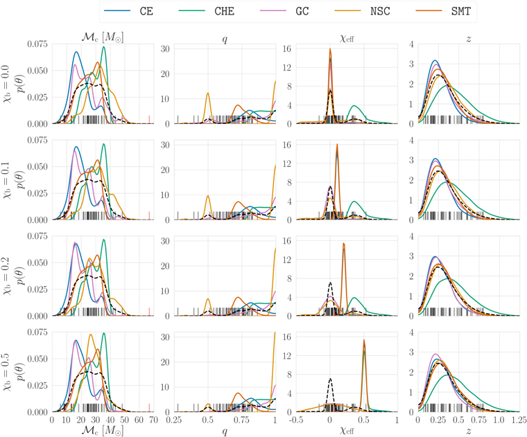
Figure 1. Marginalized detection-weighted distributions of BBH parameters for our five formation channels with varying natal spin prescriptions. The CE efficiency is fixed at αCE = 1.0 for all models in this figure. Black ticks mark the median value of the posterior distribution for all confident BBHs in GWTC-2; GW190521, which is excluded from our analysis, is instead marked with a red tick. The dashed black line shows an example mixture model synthesized for the five channels, assuming equal detectable branching fractions and a true model with the values χb = 0.0 and αCE = 1.0.
Download figure:
Standard image High-resolution image3. Population Inference
Given our astrophysical models, we now establish how we place constraints on branching fractions and physical prescriptions using the current catalog of BBH observations. We use posterior and prior samples from the GWTC-1 (Abbott et al. 2019a) and GWTC-2 (Abbott et al. 2020b) analyses, publicly available from the Gravitational Wave Open Science Center (Abbott et al. 2021). For GWTC-1 and GWTC-2, we use the Combined and PublicationSamples posterior samples, respectively, which combine posterior samples from different waveform approximants to marginalize over uncertainties in waveform modeling (Abbott et al. 2016b). The choice of prior on the event parameters is irrelevant since they are divided out during the inference. The detection probabilities for each sample in our populations are calculated assuming a detector network consisting of LIGO Hanford, LIGO Livingston, and Virgo operating at midhighlatelow sensitivity (Abbott et al. 2018) and assuming a network signal-to-noise ratio (S/N) threshold of ρthresh = 10 (see Appendix B); these detection probabilities are used to construct the detection-weighted distributions in Figure 1. We only consider high-confidence GW events that are definite mergers of two BHs, thus excluding GW170817 (Abbott et al. 2017), GW190425 (Abbott et al. 2020a), GW190426 (Abbott et al. 2020b), and GW190814 (Abbott et al. 2020d). We also exclude GW190521 (Abbott et al. 2020e) from our analysis as it has vanishing support across our models and picks up on minute fluctuations in the kernel density estimates (KDEs) for certain population models. This event is either not explainable by our set of channels or requires updated physical prescriptions for our set of channels. For each event, we randomly draw 102 samples from its posterior distribution to evaluate in the population model KDEs, which are parameterized by χb, αCE, and the formation channel. We provide additional details for our KDE generation in Appendix C.
We perform hierarchical modeling to place constraints on the parameters influencing our population models using a methodology similar to that of Zevin et al. (2017). Since we are only interested in the shape of the populations and not in the merger rate, we implicitly marginalize over the expected number of detections (e.g., Fishbach et al. 2018). The hyperparameters we wish to infer are the underlying branching fractions, β = [β CE , β CHE , β GC , β NSC , β SMT ], and the physical prescriptions assumed in each model, λ = [χb, αCE]. We assume an uninformative prior across β , given by a Dirichlet distribution with equal concentration parameters and dimensions equal to the number of formation channels, and impose the constraints (0 ≤ βi ≤ 1) ∀ i and ∑i βi = 1. Alternatively, this prior could be proportional to the predicted local merger rates for these channels; however, given the large uncertainties in the predicted merger rates we choose an uninformative prior for this work. We assume a uniform prior across the physical prescription parameters λ . 11 Since the χb and αCE models are not mixed across formation channels (i.e., the CE channel cannot have χb = 0.0, while the GC channel has χb = 0.1), this results in Nchannel + 1 hyperparameters in our modeling: two physical prescriptions and (Nchannel − 1) branching fractions, since one branching fraction is inferred given the constraint that the branching fractions sum to unity.
Given our model hyperparameters Λ = [
λ
,
β
] and the posterior samples of our event parameters ![${\boldsymbol{\theta }}=[{{ \mathcal M }}_{{\rm{c}}},q,{\chi }_{\mathrm{eff}},z]$](https://content.cld.iop.org/journals/0004-637X/910/2/152/revision2/apjabe40eieqn2.gif) , our hyperlikelihood p(
θ
∣Λ) is given by a mixture model of channels:
, our hyperlikelihood p(
θ
∣Λ) is given by a mixture model of channels:

where  is the (underlying) population model associated with βj
, parameterized by a particular natal spin magnitude and CE efficiency. Using the discrete posterior samples for each event, the likelihood of the observed GW data
is the (underlying) population model associated with βj
, parameterized by a particular natal spin magnitude and CE efficiency. Using the discrete posterior samples for each event, the likelihood of the observed GW data  given our model hyperparameters is

where Nobs is the number of GW events, Si
denotes the posterior samples used for event i, π(
θ
k
) is the prior weight for each posterior sample in the LVC analysis, and  is the detection efficiency of each hypermodel (e.g., Mandel et al. 2019; Vitale et al. 2020). The hyperposterior is thus given by

where π(Λ) is the prior on our hyperparameters.
In practice, the likelihood of Equation (2) is evaluated by first moving in the (discrete) physical prescription parameter λ space, then moving in the (continuous) branching fraction β space, and evaluating if the jump proposal is accepted. Thus, Equation (2) consists of evaluations from a mixture model of the underlying population KDEs for the given values of χb, αCE, and β at a particular step in the sampler. We use the ensemble sampler from emcee (Foreman-Mackey et al. 2013) to sample this distribution, and perform 102 realizations of this inference with different random samplings from the event posteriors, creating a combined posterior distribution across these realizations. Further details can be found in Appendix D, and results from a mock injection study using this methodology can be found in Appendix E.
4. Application to GWTC-2
4.1. Two-channel Example
We first consider a simplified picture to build intuition for the full analysis, assuming that the BBH population comes from only the CE and GC channels. The posterior distributions for the underlying branching fractions β are shown in Figure 2, with colored lines showing the contribution of various χb models to the full posteriors for
β
. In this simplified case, we already see some notable features. The Bayes factors  between models are given by the number of samples in one physical prescription model compared to another (i.e., the relative area under the colored curves in the top panels of Figure 2). We find a preference for our smallest natal spin model (χb = 0.0) relative to the higher χb models considered. Compared to the highest natal spin model (χb = 0.5), the χb = 0.0 model is preferred by a Bayes factor of
  . However, once natal spin magnitudes are decreased to lower values, the preference becomes more marginal,
  and
and  , respectively. This is consistent with the population analysis associated with GWTC-2, which pushes to low component spins for the BBH population (Abbott et al. 2020c).

Figure 2. Top row: Branching fractions between CE and GC channels, under the assumption that only these two channels contribute to the BBH catalog. Black dashed lines show the posterior on the detected branching fractions β, marginalized over the χb and αCE models. Colored lines show the contributions to the full β posterior from various χb models. Bottom row: Posterior distribution on  . The gray line shows the prior distribution for
  vertical lines mark the symmetric 90% credible interval for the fully marginalized posterior and prior distributions.
Download figure:
Standard image High-resolution imageWhen marginalizing over all values of χb and αCE, the median and symmetric 90% credible interval of the posterior distributions for β
CE
and β
GC
are  and
and  , respectively. The branching fractions are sensitive to the value of χb; we find a significant increase (decrease) in β
GC
(β
CE
) for models with χb ≥ 0.1. If we take our most extreme natal spin model, χb = 0.5, the inferred branching fractions reverse:
, respectively. The branching fractions are sensitive to the value of χb; we find a significant increase (decrease) in β
GC
(β
CE
) for models with χb ≥ 0.1. If we take our most extreme natal spin model, χb = 0.5, the inferred branching fractions reverse:  and
and  . However, this model is strongly disfavored by the data. In the bottom panel of Figure 2, we also gauge the preference for a mixture of channels in the underlying population by evaluating the posterior distribution for
  , defined as the largest value of β across all channels. We find
  (0.97) at the 90% (99%) credible level when all spin models are considered. For this simplified case, if natal spins for BHs born in isolation are low, which is favored by the data, the CE channel dominates the underlying BBH population, though some contribution from the GC channel is still necessary. These results are for the underlying population of BBHs; we discuss the conversion to the detectable population in the following section.
4.2. Five-channel Analysis
We now perform the same analysis but using all of our five formation models. In this case, we also consider the branching fractions for the detectable population  , which encodes the breakdown of formation channels to the population detected by LIGO–Virgo. To transform to such detectable branching fractions, we rescale the recovered underlying branching fractions by the detection efficiency of each population model,
  :
:

where ξ is a vector of detection efficiencies for all formation models j given a particular submodel χ,α and β ⊙ ξ is the element-wise product of β and ξ for samples in submodel χ,α. The posterior distributions for the underlying and detectable branching fractions are shown in Figures 3 and 4, respectively, with the top row breaking down the contribution from the various χb models and the bottom row breaking down the contribution from the various αCE models.
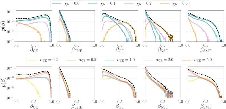
Figure 3. Branching fractions for all five channels inferred using the GWTC-2 BBHs. Colored lines show the contributions from various χb models marginalized over αCE models (top row) and various αCE models marginalized over χb models (bottom row). Black dashed lines show the full posterior on the branching fractions, marginalized over both χb and αCE models.
Download figure:
Standard image High-resolution imageEven when considering all five channels, the underlying populations may be dominated by the CE channel, though there is significant support for lower values of β
CE
and a non-negligible contribution from the other channels (see Figure 3). The median and 90% credible interval for the underlying branching fraction posteriors
β
= [β
CE
, β
CHE
, β
GC
, β
NSC
, β
SMT
] are  ,
,  ,
,  ,
,  ,
,  ]. These correspond to relative measurement uncertainties on the underlying branching fractions of ∼80%–430% (90% credibility). Though most of the distributions are broad, the CE channel has the least support at β = 0; at least 2.4% of the underlying population is from the CE channel at 99% credibility.
As expected, we also find notably different inferred branching fractions and model preferences between the two-channel case and the five-channel case. For example, as compared to that in the two-channel analysis, in the five-channel analysis the median branching fraction for the CE channel decreases by 21%, while the median branching fraction for the GC channel increases by 5%, and the χb = 0.1 model is increasingly favored by a factor of  .
.
In certain formation channels, we see the branching fractions converge to different values when different physical prescriptions are assumed. The branching fractions for dynamical (isolated) channels push to larger (smaller) values with increasing χb; moving from χb = 0.0 to χb = 0.5 leads to an increase in the median recovered branching fraction of 0.51 for the GC channel. This is due to the effective inspiral spin distribution for the BBHs in the LVC catalog, which is near-symmetric about zero although slightly skewed toward positive values (Abbott et al. 2020c). As natal spins increase, the isotropic spin orientations in dynamical environments lead to broader and symmetric effective inspiral spin distributions, whereas the relatively aligned spins from isolated evolution channels lead to a strong peak in the effective inspiral spin distributions at positive values (see Figure 1). Thus, under the assumption of nonzero natal spins, the inferred relative branching fraction between channels will change, increasing the relative contribution from dynamical formation channels. Systematic shifts in the inferred branching fractions are also apparent for variations in the CE efficiency; for the CE channel, changing αCE by an order of magnitude from 0.2 to 2.0 increases the median β CE by 0.63.
The posterior distributions on detectable branching fractions are shown in Figure 4. The median and 90% credible interval for the detectable branching fraction posteriors ![${{\boldsymbol{\beta }}}^{\det }=[{\beta }_{{\mathtt{CE}}}^{\det },{\beta }_{{\mathtt{CHE}}}^{\det },{\beta }_{{\mathtt{GC}}}^{\det },{\beta }_{{\mathtt{NSC}}}^{\det },{\beta }_{{\mathtt{SMT}}}^{\det }]$](https://content.cld.iop.org/journals/0004-637X/910/2/152/revision2/apjabe40eieqn26.gif) are
are  ,
,  ,
,  ,
,  ,
,  ]. The detectable branching fractions for all channels other than CE increase relative to the underlying branching fractions, since the CE channel typically produces BBHs with lower masses. This is due to the mass spectrum of these channels pushing to larger values, particularly for the favored χb = 0 model, which leads to an increase in their detection efficiency. Given our astrophysical models, the GC channel contributes to the bulk of the detected population, making up >2.6% of the observed population at 99% credibility. The most significant increases when converting to detectable branching fractions are in the channels whose mass spectra push to the largest values; given our set of formation models, the median detectable branching fraction for the NSC channel is almost an order of magnitude larger than the median underlying branching fraction.

Figure 4. Same as Figure 3 but with detectable branching fractions instead of branching fractions for the underlying population.
Download figure:
Standard image High-resolution imageOnce again, the detectable branching fraction for isolated channels rises with decreasing natal spin magnitude. For example, the median value for  increases by 24% when considering the χb = 0.0 model relative to the fully marginalized models.
To further gauge whether a single channel or multiple channels are favored by the BBH population, we again show the posterior distribution on  in Figure 5, now with all five formation channels included. In this higher-dimensional case, the prior on
  has a more complicated morphology; the prior volume near β = 1 for any one channel drops precipitously. However, we still see that the posterior on
  significantly deviates from the prior, pushing to larger values of
  and favoring one channel dominating the underlying population. For the underlying branching fractions, we find that
  is constrained to be below 0.88 (0.93) at the 90% (99%) credible level, compared to 0.62 (0.79) for the prior. Conversely, we find a mixture of channels contributing to the detected population to be strongly preferred. For the detectable population,
  (0.69) at 90% (99%) credibility compared to 0.75 (0.89) for the prior.
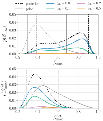
Figure 5. Posterior distribution for the maximum branching fractions of the underlying population  (top row) and detectable population
  (bottom row) when considering all five formation channel models. The black dashed line shows the fully marginalized posterior distribution, with colored lines showing the contribution to the posterior from the different χb models marginalized over all αCE models. We also show the prior distributions for
  and
and  with gray lines; vertical black dashed lines and gray lines mark the symmetric 90% credible interval for the fully marginalized posterior and prior, respectively. There is a clear difference between the branching ratios in the detectable population and the underlying population. Since higher-mass binaries are more likely to be detected, the subpopulations that contribute to these channels are enhanced, making the detectable population much more diverse.
Download figure:
Standard image High-resolution imageAnother metric we can consider is the number of channels that dominate the branching fractions. We gauge this by examining the posterior distribution on the number of branching fractions that are simultaneously above a threshold value. Setting the threshold to β = 0.1 and marginalizing over all χb and αCE models, we find that ≃26% of the posterior for the underlying branching fractions supports a single model contributing to more than 10% of the underlying population, and >95% of the posterior supports a significant contribution from three or fewer channels. Though our CE model is favored, this indicates that there may still be an appreciable contribution from a couple of other formation channels to the underlying BBH population. This picture changes drastically for the detectable population. We find that there is a >99.8% probability that more than one channel contributes to at least 10% of the detected population, with the bulk of the posterior support (≃79%) suggesting that three to four channels significantly contribute. Thus, given our astrophysical models, the detected catalog of BBHs comes from a diverse array of formation scenarios.
The Bayes factors between the physical prescriptions
λ
= [χb, αCE] are given in Table 1, analogous to the fully integrated colored curves in Figure 3. As with the two-channel case, we find moderate to strong preference for low natal spins of χb ≲ 0.1 relative to larger natal spins, in agreement with other work investigating natal spin distributions using the catalog of BBH events (Farr et al. 2017b; Abbott et al. 2020c; Kimball et al. 2020b; Miller et al. 2020). Spins of χb ≲ 0.1 are favored relative to models with χb ≳ 0.2 by a Bayes factor of  . The marginal preference for the no-spin χb = 0.0 model compared to the low-spin χb = 0.1 model (
 ) indicates no strong discriminating power between the two.
Table 1. Bayes Factors  across χb Models (Columns) and αCE Models (Rows)
| χb | ||||||
|---|---|---|---|---|---|---|
| 0.0 | 0.1 | 0.2 | 0.5 | |||
| 0.2 | −0.63 | −0.56 | −1.24 | −1.71 | −0.35 | |
| 0.5 | −0.06 | −0.58 | −0.96 | −1.11 | 0.00 | |
| αCE | 1.0 | ≡0 | −0.77 | −1.02 | −1.29 | ≡0 |
| 2.0 | 0.34 | 0.05 | −1.19 | −1.15 | 0.42 | |
| 5.0 | 0.56 | 0.39 | −0.54 | −0.87 | 0.70 | |
| ≡0 | −0.27 | −1.11 | −1.35 | |||
Notes. The Bayes factors are normalized against αCE = 1.0 and χb = 0.0 in the general case, against χb = 0.0 when marginalizing over αCE, and against αCE = 1.0 when marginalizing over χb. The bottom row provides the Bayes factors for χb models marginalized over all αCE models, and the rightmost column provides the Bayes factors for αCE models marginalized over all χb models.
Download table as: ASCIITypeset image
We also marginally prefer high CE efficiencies of αCE ≃ 5.0, which have Bayes factors of  relative to the αCE = 1.0 model. Values of αCE = 1.0 and αCE = 0.5 show near-equal preference, and highly inefficient CEs with αCE = 0.2 are disfavored relative to the most highly favored model (αCE = 5.0) by a Bayes factor of ≳10. Though we use the CE and SMT models from Bavera et al. (2020b) in this work, we find the opposite results in terms of the inferred CE efficiency. In Bavera et al. (2020b), low CE efficiencies preferentially form more massive BBHs. Since only the CE and SMT channels are considered in Bavera et al. (2020b), the preference for low CE efficiencies comes from the necessity to produce these more massive systems to match the properties of the events in GWTC-2, whereas in this work such systems can be explained by alternative formation channels. We tested this hypothesis by considering two-channel inference that included only the CE and SMT channels, and also found a strong preference for CE efficiencies of αCE ≃ 0.5, with no samples in the efficient (αCE > 1.0) CE models.
5. Discussion and Conclusions
We analyze the recently bolstered catalog of BBH mergers using a suite of state-of-the-art models for astrophysical formation channels of BBHs. Our main findings are as follows:
- 1.Though the CE channel dominates the underlying BBH population in our models, a contribution from various formation channels is preferred over one channel dominating the detected population of BBH mergers. From the formation channels considered in this work, we find that no single channel contributes to more than 70% of the detectable BBH population at 99% credibility, and the probability that three to four channels each contribute to more than 10% of the detected BBH population is 79%.
- 2.Small natal spins (χb ≲ 0.1) for BHs born in isolation or without significant tidal influence from a binary partner are favored over larger natal spins (χb ≳ 0.2) by a Bayes factor of ≃12.9, indicating efficient angular momentum transport in massive stars.
- 3.The CE efficiency, which scales roughly linearly with the post-CE separation, shows marginal preference for larger values (αCE ≃ 5.0) relative to αCE ≈ 1.0 by a Bayes factor of ≈5 and stronger preference relative to highly inefficient CEs (αCE ≃ 0.2) by a Bayes factor ≳ 10. This preference for efficient CE ejection may indicate that other energy sources are at play when ejecting CEs rather than solely the orbital energy of the binary (Ivanova et al. 2013).
- 4.When incorrect physical prescriptions are assumed or formation channels contributing to the BBH population are not considered, estimates for the values of branching fractions and variables in physical parameterizations can be significantly biased.
Numerous studies have investigated how populations of compact-object mergers can help inform uncertainties in binary stellar evolution and compact-object formation. This is typically done with either phenomenological models or predictions from population models, though in the case of the latter, usually under the assumption that a single population model is exclusively contributing to the entire population. However, several studies have considered the relative contribution and population properties expected from dynamical channels versus isolated binary evolution (e.g., Rodriguez et al. 2016b; Farr et al. 2017b; Stevenson et al. 2017a; Vitale et al. 2017; Zevin et al. 2017; Bouffanais et al. 2019; Arca Sedda et al. 2020; Safarzadeh et al. 2020; Santoliquido et al. 2020; Wong et al. 2020). For example, when considering BBH mergers formed in isolation or dynamically in young stellar clusters, Bouffanais et al. (2019) found that branching fractions can be constrained to the ∼10% level with  detections. With only ∼50 observations in GWTC-2 and the inclusion of additional formation channels, we see broader constraints on the precise values of branching fractions; the convergence on branching fraction estimates when considering more channels will be investigated in future work. Wong et al. (2020) also analyzed the BBH population from GWTC-2 using models for the GC and CE channels. We find opposite results for the underlying branching fractions when we consider the simplified picture of only the CE and GC channels (see Figure 2); we find the majority of the underlying population (∼90%) comes from the CE channel, whereas Wong et al. (2020) found ∼80% of the underlying population comes from the GC channel. However, our detectable distributions are in better agreement with the branching fractions presented in Wong et al. (2020); incorporating detectability increases the detectable branching fraction of GCs in the two-channel example to ∼70%. We also find a slight preference for efficient CEs and a stronger preference against highly inefficient CEs (αCE ≃ 0.2), whereas the constraints for αCE in Wong et al. (2020) are broad but slightly favor inefficient CEs. The difference in our analyses may be due to our inclusion of spin information, since the CE efficiency has a stronger impact on the spin distributions of the CE channel compared to the mass spectrum. This emphasizes the importance of considering all observational information when constraining models.
Though we consider five distinct BBH formation models in this analysis, we can also investigate the broad two-channel categorization of formation in the galactic field and dynamical assembly in dense stellar environments. In Figure 6, we combine the branching fractions for the field channels (CE, CHE, SMT) against the dynamical channels (GC, NSC). With low spins (χb ≲ 0.1), we find a strong preference for field channels comprising the majority of the underlying distribution. The field channels are dominated by the CE channel, which makes up the majority of the underlying population (see Figure 3). Marginalizing over all χb and αCE models, we find the underlying branching fractions for the field channels and dynamical channels are  and
and  , respectively (90% credibility). The contribution from dynamical channels increases as natal spins increase due to the behavior of the effective inspiral spin distributions, since the effective inspiral spins of the BBH events in GWTC-2 are near-symmetric about zero (Abbott et al. 2020c) and incompatible with a highly spinning, aligned-spin population. At χb = 0.5, which is disfavored relative to χb = 0 by a Bayes factor of ≃27, the underlying branching fractions are
  and
and  . In the bottom panel of Figure 6, we again use Equation (4) to convert underlying branching fractions to detectable branching fractions. In the detectable population, the contribution from dynamical channels is amplified. Marginalizing over all χb and αCE values, we find the inferred branching fractions of the detected populations to be
  and
and  . Thus, given the formation models considered in this work, dynamical and field channels contribute similar numbers to the detected BBH population.

Figure 6. Branching fractions recovered for the combined field and dynamical channels. Colored lines show the contribution to the posterior from the different χb models marginalized over all αCE models. In the top row we show the distribution for underlying branching fractions as in Figure 3, and in the bottom row we show the distribution for detectable branching fractions as in Figure 4.
Download figure:
Standard image High-resolution imageOur analysis favors low natal spins for BHs born in isolation or without significant tidal spin-up. Analyses using phenomenological representations for the spin magnitude distribution show a preference for low spins (Farr et al. 2017b; Abbott et al. 2019b, 2020c; Kimball et al. 2020b; Miller et al. 2020), in agreement with the preference for low natal spins in this work. Low spins in the natal population will increase the rate of hierarchical mergers in dynamical environments (Rodriguez et al. 2019; Banerjee 2021; Fragione & Loeb 2021; Fragione & Silk 2020; Kimball et al. 2020a), pushing the BH mass spectrum to larger values, imparting large spin on the merger products, and accentuating the mass asymmetry of mergers in those populations.
We find a mild preference for efficient CEs in our modeling, which strongly disfavors highly inefficient CEs with αCE ≃ 0.2. Inferred values for the CE efficiency αCE have more diversity than natal spins across the literature, from population modeling (e.g., Bavera et al. 2020b; Santoliquido et al. 2021; Zevin et al. 2020) to hydrodynamical simulations (e.g., Fragos et al. 2019) and theoretical considerations (e.g., Ivanova et al. 2013). Our results, which mildly favor high CE efficiencies, are in agreement with Santoliquido et al. (2021), who found high CE efficiencies are necessary to match the merger rate of binary neutron stars in their population models, and with Fragos et al. (2019), who modeled the spiral-in phase of CE evolution using hydrodynamic simulations and found a non-negligible fraction of the envelope remains bound to the core after the CE is successfully ejected. These results for αCE contrast with those from Bavera et al. (2020b), but we find that these conflicting results arise only from the consideration of more formation channels in this work; when considering contributions from only the CE and SMT channels, we also favor low CE efficiencies of αCE ≃ 0.5. We also find similar detectable branching fractions for the CE and SMT channels, in agreement with Bavera et al. (2020b), who found the channels have comparable BBH detection rates in the local universe.
We have shown multiple times that failing to account for the broad array of formation channels or assuming incorrect physical prescriptions can severely bias inferences. For example, when only considering the CE and SMT channels in our inference, we find a preference for low CE efficiencies compared to the preference for high CE efficiencies when considering all five channels. When considering only the CE and GC channels, the recovered branching fractions differ significantly compared to when we consider all five channels (see Figures 2 and 3). Even when including our full array of formation channels, differing assumptions for physical prescriptions alter the recovered branching fractions (see Section 4.2).
While we consider more formation channels in this analysis than has been done before, the astrophysical models used in this work only comprise a subset of the proposed formation channels for BBHs, 12 and each channel is subject to a number of additional theoretical uncertainties that are not accounted for in this work. Therefore, as with any such model selection endeavor that is reliant on population modeling predictions, there are a number of inherent caveats associated with assumptions made for uncertain physical prescriptions. A few examples of such caveats are as follows: (a) since a massive-star binary in a CE phase has never been observed, the modeling of this phase is entirely theoretical, and the α–λ energy balance formalism with a fixed CE efficiency αCE across all stellar regimes may not be valid; (b) BH natal kick magnitudes and orientations relative to the spin axis of the exploding star are uncertain due to the limited observational sample of BH binaries with well-measured proper motions, and choosing a natal kick prescription other than the standard bimodal Maxwellian distribution with fallback-modulated kicks can affect both population properties and rates; (c) using a fixed natal spin for isolated BHs, which is a proxy for the efficiency of angular momentum transport, may instead be better described by a distribution of natal spins dependent on the properties of the collapsing star; and (d) in clusters, changes in the assumed binarity of the primordial population, cluster rotation, triaxiality, and the dynamical effect that would be caused by the presence of a massive BH may all have an impact on the properties of BBH mergers. This list of caveats is not exhaustive, but it provides a sense of the complexity of this model selection problem, especially when considering contributions from multiple formation scenarios that have both shared and independent physical uncertainties. Though our quantitative results may change with the inclusion of additional formation models or updated prescriptions for binary stellar evolution and compact-object formation, given the diversity of BBH detections to date we anticipate that the necessity for multiple channels significantly contributing to the detected BBH population is robust. Since the local BBH merger rate continues to become more constrained as the catalog of BBHs grows, predicted merger rates will also be crucial to include in these types of analyses and can be incorporated into branching fraction priors.
As statistical uncertainties get smaller, systematics become more important (Barrett et al. 2018), and failing to consider a more complete and comprehensive picture for the diversity of possible BBH formation channels will become increasingly dangerous. As the detected population of BBHs grows, our methodology can be expanded to include additional formation channels and uncertain physical prescriptions, which will lead to a more unbiased and complete understanding of the relative contribution from various astrophysical channels to the observed population of compact binary mergers. Only through these comprehensive analyses will we be able to accurately infer crucial aspects of BBH origins.
The population models and posterior samples from the hierarchical inference in this work are available on Zenodo (Zevin 2020). The codebase developed for this analysis, Astrophysical Model Analysis and Evidence Evaluation (AMA
 E), is available on Github
13
along with notebooks for generating the numbers and figures in this paper.
E), is available on Github
13
along with notebooks for generating the numbers and figures in this paper.
The authors would like to thank Tom Callister and Maya Fishbach for their useful suggestions and to acknowledge the thoughtful comments from the anonymous referees, which helped improve this paper. Support for this work and for M.Z. was provided by NASA through the NASA Hubble Fellowship grant HST-HF2-51474.001-A awarded by the Space Telescope Science Institute, which is operated by the Association of Universities for Research in Astronomy, Inc., for NASA, under contract NAS5-26555. S.S.B. and T.F. are supported by a Swiss National Science Foundation professorship grant (project No. PP00P2 176868). This project has received funding from the European Union's Horizon 2020 research and innovation program under the Marie Sklodowska-Curie RISE action, grant agreement No. 691164 (ASTROSTAT). C.P.L.B. is supported by the CIERA Board of Visitors Research Professorship and National Science Foundation (NSF) grant PHY-1912648. V.K. is supported by a CIFAR G+EU Senior Fellowship and Northwestern University. P.M. acknowledges support from FWO junior postdoctoral fellowship No. 12ZY520N. F.A. acknowledges support from a Rutherford fellowship (ST/P00492X/1) from the Science and Technology Facilities Council. D.E.H. was supported by NSF grants PHY-1708081 and PHY-2011997, the Kavli Institute for Cosmological Physics at the University of Chicago, and an endowment from the Kavli Foundation and also gratefully acknowledges a Marion and Stuart Rice Award. This work used computing resources at CIERA funded by NSF grant No. PHY-1726951 and resources and staff provided by the Quest high-performance computing facility at Northwestern University, which is jointly supported by the Office of the Provost, the Office for Research, and Northwestern University Information Technology. This document has been assigned LIGO document No. LIGO-P2000468. 14
Software:
Astropy (Robitaille et al. 2013; Price-Whelan et al. 2018); emcee (Foreman-Mackey et al. 2013); iPython (Pérez & Granger 2007); Matplotlib (Hunter 2007); NumPy (Oliphant 2006; Van Der Walt et al. 2011); Pandas (McKinney 2010); PyCBC (Nitz et al. 2019); SciPy (Virtanen et al. 2020); AMA
 E (this work).
Appendix A: Population Models
In this section, we provide further details for the population modeling in this work. In Appendix A.1, we discuss the formation channels used in our inference and the assumptions that were made to provide more self-consistency between models. In Appendix A.2, we discuss the distribution of systems across cosmic time for our five formation channels, as well as the assumed distribution of metallicities as a function of redshift.
A.1. Formation Channels
A.1.1. Isolated Evolution through CE and Stable Mass Transfer
The CE and SMT models are simulated with the POSYDON framework (T. Fragos et al. 2021, in preparation), which was used to combine the rapid population synthesis code COSMIC (Breivik et al. 2020) with MESA detailed binary evolution calculations (Paxton et al. 2011, 2013, 2015, 2018, 2019) as in Bavera et al. (2020b). COSMIC was used to rapidly evolve binaries from the zero-age main sequence until the end of the second mass-transfer episode. For the last phase of the binary evolution (BH–Wolf–Rayet), which determines the second-born BH spin (Qin et al. 2018; Bavera et al. 2020a), we used detailed stellar and binary simulations from MESA. These simulations take into account differential stellar rotation, tidal interaction, stellar winds, and the evolution of the Wolf–Rayet stellar structure, therefore allowing us to carefully model the tidal spin-up phase until the core collapse of the secondary.
These models assume the first-born BH is formed with a negligible spin χb ≃ 0 because of the assumed efficient angular momentum transport (Qin et al. 2018; Fuller & Ma 2019) and the Eddington-limited accretion efficiency onto compact objects; this also leads to small first-born BH spins for the SMT channel because the mass accreted onto BHs during the second mass transfer is negligible (Thorne 1974). In this work we artificially varied the first assumption by changing the birth spins in post-processing. Assumptions for the efficiency of accretion onto BHs may affect the natal spins of the first-born BH in the SMT channel if it is highly super-Eddington, though Bavera et al. (2020b) showed that a highly super-Eddington accretion efficiency leads to the extinction of BBH mergers in the SMT channel and thus we do not consider variations in its value.
These simulations were designed as much as possible to match the same stellar and binary physical assumptions made in the CHE models; in fact, the MESA model is entirely self-consistent with that used in du Buisson et al. (2020). Consistency in the initial binary distributions was also a priority. For example, we assumed that log-initial orbital period distributions follow a Sana et al. (2012) power law in the range [100.15, 105.5] days and extend down to 0.4 days assuming a flat-in-log distribution in order to sample the parameter space leading to a chemically homogeneous evolution (du Buisson et al. 2020). Finally, analogous to the CHE and NSC models, we used the same prescriptions for distributing the synthetic BBH populations across cosmic history (see Appendix A.2). To translate the underlying BBH population to the detected population in all channels, Bavera et al. (2020b) assumed the detection probabilities detailed in Appendix B but with a higher network S/N threshold of ρthresh = 12. The estimated rate densities for the CE channel are in the range 17–113 Gpc−3 yr−1 depending on αCE (the smallest value corresponds to the model with αCE = 5.0, while the largest value corresponds to αCE = 0.2) and 25 Gpc−3 yr−1 for the SMT channel (Bavera et al. 2020b). For a detector network with midhighlatelow sensitivity and a network detection threshold of ρthresh = 12, these values translate to a detection rate of 15–412 yr−1 and 86 yr−1 for CE and SMT, respectively.
A.1.2. Chemically Homogeneous Evolution
The CHE models are adopted from du Buisson et al. (2020), who computed a large grid of detailed MESA stellar and binary simulations undergoing this evolutionary process. For consistency with the other models, we restrict primary masses to the range [0.01, 150] M⊙, meaning that, compared to the original study, we ignore systems forming BBHs with components above the pair instability mass gap (e.g., Woosley 2017; Farmer et al. 2019; Marchant et al. 2019). The core collapse of the stars' profiles is done self-consistently in CE and SMT models using POSYDON (see Appendix D of Bavera et al. 2020b). The applied prescription takes into account disk formation during the collapse of highly spinning stars, mass loss through neutrinos, (pulsational) pair instability supernovae according to the fits of the detailed simulation of Marchant et al. (2019), and two Blaauw kicks (Blaauw 1961; Kalogera 1996) where we assume circularization after the first supernova (see du Buisson et al. 2020). The synthetic population of BBHs is distributed across cosmic history assuming the same initial binary distributions in the CE and SMT models.
Since we have a regular grid of MESA simulations covering the initial binary distributions instead of sampling them with a Monte Carlo approach, we can directly calculate their phase space volume. Given a binary k with initial primary mass m1,k , mass ratio qk , and period pk , the relative contribution of that system to the total population Pk is
where IMF, IQF, and IPF designate the initial mass, mass ratio, and period functions. These probabilities are obtained by integrating the assumed initial distribution probability densities independently; for simplicity, we assume that the initial binary properties are independent of each other and of metallicity. For the initial mass function, we assume a Kroupa (2001) power law in the range [0.01, 150] M⊙; for the initial mass ratios, we assume a flat distribution in the range [0, 1]; and for the initial periods, we assume an extended Sana et al. (2012) log-power law as in Equation (A.1) of Bavera et al. (2020b). For each binary the integration is performed around the initial values m1,k
, qk
, and pk
assuming a volume corresponding to the grid's resolution, namely,  , Δqk
= 0.2, and Δ(pk
/day) = 0.025. Even though the simulations for the CHE channel were carried out at a fixed mass ratio value of q = 1, here we assume that they are representative of resultant BBH mass ratios within [0.8, 1], and artificially smear the BBH mass ratios uniformly across this range while keeping the total mass of the binary fixed. This assumption is justified by the findings of Marchant et al. (2016).
, Δqk
= 0.2, and Δ(pk
/day) = 0.025. Even though the simulations for the CHE channel were carried out at a fixed mass ratio value of q = 1, here we assume that they are representative of resultant BBH mass ratios within [0.8, 1], and artificially smear the BBH mass ratios uniformly across this range while keeping the total mass of the binary fixed. This assumption is justified by the findings of Marchant et al. (2016).
Similar to Equation (7) of Bavera et al. (2020b), the BBH merger rate density is calculated in finite-time bins of Δti = 100 Myr and log-metallicity bins ΔZj where each binary k is placed at the center of each time bin corresponding to the redshift of formation zf,i and merging at zm,i,k . Therefore,
where fbin = 0.7 (Sana et al. 2012) is the binary fraction,  is the average system mass (computed as in Equation (A.2) of Bavera et al. 2020a), fSFR is the star formation rate (SFR) per metallicity range ΔZj
, Dc(z) is the comoving distance, and ΔVc is the comoving volume corresponding to Δti
. Using a network detection threshold of ρthresh = 12, we find a merger rate density of 32.9 Gpc−3 yr−1 and a detection rate for a detector network with midhighlatelow sensitivity of 360 yr−1. The rate found here is higher than the one found by du Buisson et al. (2020), 5.8 Gpc−3 yr−1, for two reasons: (i) The original study assumed a flat-in-log orbital period distribution over the range [0.4, 365.25] days compared to the extended log-power law assumed here for consistency with the CE and SMT channels; when we assume the original distribution over the range [0.4, 105.5] days, the rate density decreases to 10.6 Gpc−3 yr−1. (ii) du Buisson et al. (2020) assumed an SFR and metallicity distribution from the cosmological simulations of Taylor & Kobayashi (2015), which predicts less stellar mass formed at low metallicities compared to Madau & Fragos (2017), assuming the metallicities follow a truncated log-normal distribution around the empirical mean of Madau & Fragos (2017) and a standard deviation of 0.5 dex.
is the average system mass (computed as in Equation (A.2) of Bavera et al. 2020a), fSFR is the star formation rate (SFR) per metallicity range ΔZj
, Dc(z) is the comoving distance, and ΔVc is the comoving volume corresponding to Δti
. Using a network detection threshold of ρthresh = 12, we find a merger rate density of 32.9 Gpc−3 yr−1 and a detection rate for a detector network with midhighlatelow sensitivity of 360 yr−1. The rate found here is higher than the one found by du Buisson et al. (2020), 5.8 Gpc−3 yr−1, for two reasons: (i) The original study assumed a flat-in-log orbital period distribution over the range [0.4, 365.25] days compared to the extended log-power law assumed here for consistency with the CE and SMT channels; when we assume the original distribution over the range [0.4, 105.5] days, the rate density decreases to 10.6 Gpc−3 yr−1. (ii) du Buisson et al. (2020) assumed an SFR and metallicity distribution from the cosmological simulations of Taylor & Kobayashi (2015), which predicts less stellar mass formed at low metallicities compared to Madau & Fragos (2017), assuming the metallicities follow a truncated log-normal distribution around the empirical mean of Madau & Fragos (2017) and a standard deviation of 0.5 dex.
A.1.3. Globular Clusters
The GC models are simulated using the Hénon-style cluster Monte Carlo code CMC (Hénon 1971a, 1971b; Joshi et al. 2000; Pattabiraman et al. 2013). CMC has been shown to reproduce both the global cluster properties and the BBH populations found in direct N-body cluster models in a fraction of the time (Rodriguez et al. 2016b). Each cluster model contains all of the necessary physics to describe the dynamical formation of BBHs. Each star and binary in the cluster is evolved with the Binary Stellar Evolution package of Hurley et al. (2000, 2002) with updated prescriptions for stellar winds, compact-object masses, supernova natal kicks, and pulsational-pair instability physics consistent with COSMIC (Chatterjee et al. 2010; Rodriguez et al. 2016a, 2018b, and references therein). The three-body interactions between single stars that produce many BBHs are treated probabilistically using prescriptions from Morscher et al. (2013), which have been well tuned to direct N-body integrations. Furthermore, stars and binaries are allowed to interact through strong three- and four-body encounters, whose outcomes are directly integrated with Fewbody (Fregeau & Rasio 2007), a small-N dynamical integrator with relativistic corrections (Antognini et al. 2014; Amaro-Seoane & Chen 2016; Rodriguez et al. 2018b). BBHs that merge inside the cluster, either as isolated systems or due to prompt GW emission during three-body encounters, are given new masses, spins, and GW recoil velocities taken from numerical relativity-based fitting formulae (Rodriguez et al. 2018b, Appendix A).
As the natal spins of BHs are set at the start of the simulations, no post-processing is necessary across our χb models. We do not consider differing αCE values in our GC models for two reasons: (i) Most BBHs that go on to merge are processed dynamically and go through partner swaps throughout their evolution in the cluster and do not merge with their original partner; thus the post-CE separation has a minimal impact on the rates and properties of BBH mergers. (ii) Of the BHs in the cluster originally in a BBH system that formed from a massive-star binary progenitor, we find only a percent-level number that were at tight enough orbital configurations during the BH–Wolf–Rayet phase for tidal spin-up to be relevant. We therefore set the CE efficiency to our fiducial value of αCE = 1 in the GC model.
The GC model is the only model that does not follow the standard star formation and metallicity evolution described in Appendix A.2, since cluster formation does not mimic the star formation history of the host galaxies. We instead follow the prescriptions in Rodriguez & Loeb (2018), which rely on detailed modeling of GC formation across cosmic time (El-Badry et al. 2019), and weight GCs of differing metallicities by the metallicity distribution of GCs observed in the Milky Way (Harris 2010).
A.1.4. Nuclear Star Clusters
The evolution of NSC models is determined using the semi-analytical approach of Antonini et al. (2019). In this method, we assume that the energy generated by the BH binaries in the cluster core is regulated by the process of two-body relaxation in the bulk of the system (Breen & Heggie 2013). This principle of balanced evolution (Hénon 1961) is used to compute the hardening and the merger rate of the core binaries. Moreover, we neglect mass loss from stellar evolution and the escape of BHs and stars, i.e., we assume a constant cluster mass (see Antonini & Gieles 2020b for caveats in this assumption). Each BBH formed dynamically in the cluster core is then evolved until it either merges inside the cluster or is ejected from it. If the merger remnant is retained inside the cluster, we compute its spin and mass using the prescriptions in Rezzolla et al. (2008). We evolve the cluster until either all BHs have been ejected or a time of 13 Gyr has passed.
As with the GC model, we do not consider differing αCE values for the NSC model and assume the population properties are the same across all values of αCE (see discussion in Appendix A.1.3). In contrast to those in the GC model, we assume that star formation and metallicity evolution follow the same prescriptions as the CE, CHE, and SMT models (i.e., they trace the evolution of the host galaxy as a whole). There are arguments that the star formation histories of nuclear clusters are different from those of their galactic hosts (Neumayer et al. 2020). Given the uncertainties, however, we continue with the assumption above and sample from the three metallicity models (0.01Z⊙, 0.1Z⊙, and 1Z⊙) according to the prescriptions described in Appendix A.2.
A.2. Formation Rate and Metallicity Evolution
All formation channels provide raw samples of BBH mergers for a given χb, αCE, and metallicity. For all models other than GC (see Appendix A.1.3), we distribute the synthetic BBH populations across cosmic history assuming the SFR density in Madau & Fragos (2017):
This determines the birth redshift of the BBH progenitor. For the CE, CHE, and SMT models, the merger redshift is then calculated using the BBH formation time (tbirth − tBBH) and inspiral time (tinsp), the latter of which is determined using the orbital properties of the binary following the birth of the second BH (Peters 1964). Thus, the merger redshift is

where  is the transformation function between the lookback time and redshift. For the NSC model, delay times (tdelay = tBBH + tinsp) are computed directly from the model and used to determine the merger redshift. For all models, we assume a ΛCDM cosmology with the Planck 2015 cosmological parameters of H0 = 68 km s−1 Mpc−1, Ωm = 0.31, and ΩΛ = 0.69 (Ade et al. 2016).
Each formation channel model is simulated across a range of metallicities. At a given redshift, metallicities are distributed following a truncated log-normal metallicity distribution around the empirical median metallicity from Madau & Fragos (2017) assuming a standard deviation of 0.5 dex (Bavera et al. 2020b, Section 2.2):

with a solar metallicity of Z⊙ = 0.017 (Grevesse & Sauval 1998). We use the SFR density, Equation (A3), and metallicity distribution, Equation (A5), to construct a full cosmological population for each submodel of the formation channels (parameterized by χb and αCE).
Appendix B: Detection Probabilities
In our inference, detection probabilities are a key component of the detection efficiency ξ in the hyperlikelihood. From the cosmological populations of each channel, we calculate detection probabilities numerically. Though this is more computationally intensive than using analytical scaling relations that approximate the sensitive spacetime volume to leading order (e.g., Fishbach & Holz 2017), we choose to calculate detection probabilities numerically to better capture the influence that the total mass, mass ratio, and spins have on selection effects.
Each system is characterized by its (source-frame) component masses, three-dimensional component spin vectors, and merger redshift. For every system in each population model, we first calculate the optimal S/N ρopt for LIGO Hanford, LIGO Livingston, and Virgo operating at midhighlatelow sensitivity (Abbott et al. 2018) by assuming the system is directly overhead with a face-on inclination. We use the IMRPhenomPv2 waveform approximant (Hannam et al. 2014; Khan et al. 2016) for determining S/N, and detector response functions are constructed using the PyCBC package (Nitz et al. 2019). We approximate the optimal network S/N as the quadrature sum of the optimal S/N from the three detectors,

which will give us a conservative overestimate of the true optimal S/N of the network. We choose a network S/N threshold of ρthresh = 10, consistent with the false-alarm-rate threshold of two per year, which is used as a criterion for events in GWTC-2 (Abbott et al. 2018, 2020b; Nitz et al. 2020). If ρnet,opt < ρthresh, we set the detection probability of the system to  . Otherwise, we consider the source potentially detectable and perform 103 Monte Carlo realizations of the extrinsic parameters, namely the right ascension, declination, inclination, and polarization angle. The detection probability of the system marginalized over the extrinsic parameters is then given by

where N is the number of Monte Carlo realizations, i indexes over detectors, ψj
denotes the extrinsic parameters drawn for the Monte Carlo sample j, and  is the Heaviside step function. These detection weights are used to construct the weighted KDE models in Figure 1.
Appendix C: KDEs of Models
We use an adaptation of the Gaussian_kde class of SciPy to construct KDEs for each population model, which are four-dimensional over the parameters θ . Our Gaussian_kde class handles reflection over physical boundaries in the parameter space (i.e., 0 < q ≤ 1). To ensure an adequate choice of KDE bandwidth for our population models, we perform a holdout analysis where we construct the KDE using a subset of samples from the full population, draw samples from the KDE, and compare the one-dimensional marginalizations of the parameters θ drawn from the KDE with another subset of samples. We find a bandwidth of ≈ 0.01 consistently matches the true distribution of parameters, whereas values lower and higher tend to overfit and underfit the data, respectively.
Appendix D: Population Inference
Our goal is to recover the posterior for our set of hyperparameters,
β
= [β
CE
, β
CHE
, β
GC
, β
NSC
, β
SMT
] and
λ
= [χb, αCE], given the set of (independent) GW observations of BBHs from GWTC-2,  . In the following, we are only interested in the shape of the populations and not the rate and implicitly marginalize out the rate term by assuming a p(N) ∝ 1/N prior on the number of detections (Fishbach et al. 2018).
Starting from the ground up, the probability of detecting a set of event parameters θ = { θ i } given the model hyperparameters Λ = [ β , λ ] from independent observations is
where  is the detection probability for an event with parameters
θ
(Chennamangalam et al. 2013; Farr et al. 2015; Mandel et al. 2019; Vitale et al. 2020). Marginalizing over event parameters, the probability of observing the data for event
x
i
given our hyperparameters Λ is
is the detection probability for an event with parameters
θ
(Chennamangalam et al. 2013; Farr et al. 2015; Mandel et al. 2019; Vitale et al. 2020). Marginalizing over event parameters, the probability of observing the data for event
x
i
given our hyperparameters Λ is

By applying Bayes' theorem, we replace p( x i ∣ θ ) with p( θ ∣ x i )p( x i )/π( θ ). Assuming independent observations, we get
where π(
θ
) is the prior on the parameters ![${\boldsymbol{\theta }}=[{{ \mathcal M }}_{{\rm{c}}},q,{\chi }_{\mathrm{eff}},z]$](https://content.cld.iop.org/journals/0004-637X/910/2/152/revision2/apjabe40eieqn63.gif) assumed in the original inference of
θ
, which is provided alongside the LVC posterior samples. We evaluate π(
θ
) at each point
θ
i
in a four-dimensional prior KDE constructed using the LVC prior samples. Since we use Si
posterior samples to approximate p(
θ
i
∣
x
i
), we can rewrite this integral as a discrete sum over the posterior samples:
assumed in the original inference of
θ
, which is provided alongside the LVC posterior samples. We evaluate π(
θ
) at each point
θ
i
in a four-dimensional prior KDE constructed using the LVC prior samples. Since we use Si
posterior samples to approximate p(
θ
i
∣
x
i
), we can rewrite this integral as a discrete sum over the posterior samples:
The hyperlikelihood  is evaluated as a mixture model of the underlying KDEs in the current χb and αCE model,

where the summation is over the formation channels and  is the χb and αCE model that the sampler is in at a given step in the chain. Thus, our hyperlikelihood from Equation (D4) becomes
where for convenience we define  , where

is the detection efficiency for each formation channel model with natal spin χ and CE efficiency α. The channel-dependent detection efficiency  is evaluated using a Monte Carlo approach, since detection probabilities are already calculated for each sample in the population models. Finally, the posterior distribution on the hyperparameters, p(Λ∣
x
) = p(
x
∣Λ)π(Λ)/p(
x
), is
is evaluated using a Monte Carlo approach, since detection probabilities are already calculated for each sample in the population models. Finally, the posterior distribution on the hyperparameters, p(Λ∣
x
) = p(
x
∣Λ)π(Λ)/p(
x
), is
where π(Λ) is the prior on the hyperparameters.
For priors, we use a Dirichlet distribution with equal concentration parameters and dimensions equal to the number of formation channels as a prior for the branching fractions β , imposing the constraints (0 ≤ βi ≤ 1) ∀ i and ∑i βi = 1. In practice, the discrete χb and αCE models are sampled using dummy index parameters that are defined on the range [0, Nλ,m ], where Nλ,m is the number of m = χb or n = αCE models, with a flat prior across this range and no support outside this range. The λ model considered at each step is given by the floor of the dummy parameter values that correspond to χb and αCE.
Appendix E: Testing with Mock Observations
In addition to examining constraints on the GW population, we can test our methodology using mock draws from the underlying population distributions. In Figures 7 and 8, we show the convergence on detectable branching fractions and physical prescriptions as the number of observations increases. In this mock sample, we set the true physical prescriptions to χb = 0.0 and αCE = 1.0 and the detectable branching fractions between channels to ![$[{\beta }_{{\mathtt{CE}}}^{\det },{\beta }_{{\mathtt{CHE}}}^{\det },{\beta }_{{\mathtt{GC}}}^{\det },{\beta }_{{\mathtt{NSC}}}^{\det },{\beta }_{{\mathtt{SMT}}}^{\det }]=[0.3,0.1,0.3,0.1,0.2]$](https://content.cld.iop.org/journals/0004-637X/910/2/152/revision2/apjabe40eieqn68.gif) . We draw systems from the underlying distributions of the various populations until
. We draw systems from the underlying distributions of the various populations until  detectable samples are drawn from channel j, where Nobs is the number of observed events for a particular mock realization. Figure 7 shows the contribution to branching fraction posteriors for different χb models, marginalized over αCE models, and Figure 8 shows the contribution to branching fraction posteriors for different αCE models, marginalized over χb models. For demonstration purposes, in these examples we assume no measurement uncertainty; in actuality the inclusion of mock measurement uncertainty will lead to less precise measurements. In this simplified example, we find our analysis recovers the injected model, with increasing Bayes factors for the correct physical prescription and increasing precision in the branching fraction measurement as the number of observations increases. As with our analysis using the GW observations, we see strong biases in the recovered branching fractions when the incorrect physical prescriptions are considered. A more investigative analysis with the inclusion of S/N-dependent measurement uncertainty will be explored in future work.

Figure 7. Convergence on underlying branching fractions using mock observations from the population models. In this example, the injected model has χb = 0, αCE = 1.0, and ![${{\boldsymbol{\beta }}}^{\det }=[0.3,0.1,0.3,0.1,0.2]$](https://content.cld.iop.org/journals/0004-637X/910/2/152/revision2/apjabe40eieqn70.gif) . Different colors show the contribution of different χb models to the full branching fraction posteriors, marginalized over αCE models; the injected χb model is shown with the blue curve. The Bayes factors between the physical models are the relative areas under the colored curves.
. Different colors show the contribution of different χb models to the full branching fraction posteriors, marginalized over αCE models; the injected χb model is shown with the blue curve. The Bayes factors between the physical models are the relative areas under the colored curves.
Download figure:
Standard image High-resolution image
Figure 8. Same as Figure 7, but the different colors show the contribution of different αCE models to the full branching fraction posteriors, marginalized over χb models. The injected αCE model is shown with the light blue curve.
Download figure:
Standard image High-resolution image
Footnotes
- 11
In practice, we use a continuous dummy parameter to evaluate the discrete model space—see Appendix D.
- 12
We welcome additional models that could be included in this framework.
- 13
- 14