


Abstract
We searched for shocked carbon chain chemistry (SCCC) sources with C3S abundances surpassing those of HC5N toward the dark cloud L1251, using the Effelsberg telescope at the K band (18–26 GHz). L1251-1 and L1251-3 are identified as the most promising SCCC sources. The two sources harbor young stellar objects. We conducted mapping observations toward L1251-A, the western tail of L1251, at λ ∼ 3 mm with the Purple Mountain Observatory 13.7 m and the Nobeyama Radio Observatory 45 m telescopes in lines of C2H, N2H+, CS, HCO+, SO, HC3N, and C18O as well as in CO 3–2 using the James Clerk Maxwell Telescope (JCMT). The spectral data were combined with archival data including Spitzer and Herschel continuum maps for further analysis. Filamentary substructures labeled as F1–F6 were extracted in L1251, with F1 being associated with L1251-A hosting L1251-1. The peak positions of dense gas traced by HCO+ are misaligned relative to those of the dust clumps. Episodic outflows are common in this region. The twisted morphology of F1 and velocity distribution along L1251-A may originate from stellar feedback. SCCC in L1251-1 may have been caused by outflow activities originated from the infrared source IRS1. The signposts of ongoing SCCC and the broadened line widths of C3S and C4H in L1251-1 as well as the distribution of HC3N are also related to outflow activities in this region. L1251-1 (IRS1) together with the previously identified SCCC source IRS3 demonstrate that L1251-A is an excellent region to study SCCC.
Export citation and abstract BibTeX RIS
1. Introduction
Carbon chain molecules (CCMs) are particularly interesting since they are important tracers of organic interstellar chemistry. The nitrogen-bearing CCMs HC3N J = 1–0 and HC5N J = 4–3 were first detected toward Sgr B2 in the 1970s (Turner 1971; Morris et al. 1976). Soon after, HC7N and HC9N were found in TMC-1 (Kroto et al. 1978; Broten et al. 1978). They are important players in hydrocarbon chemistry (Dickens et al. 2001) and constrain evolutionary stages of dark cold cores (Benedettini et al. 2012). These molecular species can also trace dynamical motions in molecular clouds, including material infall (Friesen et al. 2013). In some cold clouds, cyanopolyynes (HC2n+1 N) are particularly prominent and even HC11N has been detected in TMC-1. (Loomis et al. 2021). In star-forming regions, cyanopolyynes are usually suppressed, although they can be abundant in some massive star-forming regions (Taniguchi et al. 2019).
Another important kind of unsaturated CCMs, sulfur-bearing molecules, including C2S and C3S, can be used to investigate the physical conditions of their production regions. In early cold cores, the column densities of sulfur-bearing molecules are usually positively correlated with those of nitrogen-containing molecules (Hirahara et al. 1992; Suzuki et al. 1992; Fuente et al. 2016). In embedded low-mass protostars, significant positive correlations between the cyanopolyynes (HCnN) and pure hydrocarbon chains (CnH) have been found (Law et al. 2018). C2S lines were not or only marginally detected in a number of low-mass star formation cores (Suzuki et al. 1992).
In L1527 (IRAS 04368+2557), Sakai et al. (2008a) and Sakai et al. (2008b) found strong emissions of high-extinction lines (Eu > 20 K) of unsaturated hydrocarbons, including C4H2, C4H, and l-C3H2. A mechanism referred to as warm carbon chain chemistry (WCCC) was put forward to explain the phenomena. In the picture of WCCC, prestellar objects contract and heat the surrounding dust, and the evaporated CH4 reacts with C+ to produce CCMs (Sakai et al. 2008b, 2009). The second WCCC source (I15398-3359) was found in Lupus I (Sakai et al. 2009). Molecular outflows were found in both WCCC sources (Sakai et al. 2008b; Oya et al. 2014; Yıldız et al. 2015). The excitation temperatures of hydrocarbons, such as C4H2 and CH3CCH, have been determined to be about 12 K in both WCCC sources (Sakai et al. 2008a, 2009), which are lower than the sublimation temperature of CH4 (25 K) but much higher than the excitation temperature of hydrocarbons in TMC-1 (3.8–6.7 K for C4H2; Kaifu et al. 2004; Sakai et al. 2008b).
Recently, we have observed six outflows and five starless Lupus cores using the Shanghai 65 m Tian Ma Radio Telescope to explore the production region and excitation mechanism of CCMs (Wu et al. 2019a). All the targets are located within 330 pc from the Earth. The HC3N J = 2–1, HC5N J = 6–5, HC7N J = 14–13, 15–14, 16–15, and C3S J = 3–2 transitions have been observed. These lines were detected toward 10 of the 11 observed sources. Three sources, IRAS 20582 + 7724 (I20582), L1221, and L1251-A (corresponding to IRS3 in the L1251-A region, hereafter L1251-IRS3), were explained in terms of a new chemical mechanism—shocked carbon chain chemistry (SCCC); another outflow source, the eastern molecular core of the outflow source L1489 (L1489 EMC) was identified as a particular carbon-chain production region and as a candidate of a WCCC source (Wu et al. 2019b).
The main concept of SCCC is that the sulfur ions and atoms released from grain surfaces under the effect of shocks will mix with cold gas components and drive a new generation of CCMs, especially the sulfur-bearing ones such as C3S. The criteria of SCCC include relatively weak N-bearing CCM emissions in contrast to strong C3S emissions and signs of developed shock regions. Our model (Wu et al. 2019a) forecasts that, in sources where the SCCC mechanism works most efficiently, the abundance of C3S (X(C3S)) will not only exceed that of HC7N (X(HC7N)), but also that of HC5N (X(HC5N)). The observations presented by Wu et al. (2019a) show that so far three known SCCC sources (IRAS 20582+7724 (I20582), L1221, and L1251-IRS3) all have N(C3S) < N(HC5N), while L1251-IRS3 possesses a C3S column density closest to but still not exceeding that of HC5N.
In this work, we further search for and examine SCCC sources in the L1251 region (see Table 1), using the Effelsberg 100 m telescope in the K band (18–26 GHz). We mapped multiple lines toward the most promising SCCC candidate (L1251-1) located in the tail of the L1251 region, using the Purple Mountain Observatory (PMO) 13.7 m and the Nobeyama Radio Observatory (NRO) 45 m telescopes in the 3 mm band as well as the James Clerk Maxwell Telescope in CO J = 3–2 (see Section 2). In Section 3, we introduce L1251, including its morphology and structure as well as the star formation activities in L1251-A. The results of our search for new SCCC sources in the L1251 region are presented in Section 4, while the results of further mapping observations toward L1251-A are presented in Section 5. In Section 6, we discuss the filamentary structures in L1251-A and SCCC-related phenomena in this region. Section 7 provides a summary.
Table 1. The Infrared and Far-infrared Continuum Flux (in Units of Millijansky) of Young Stellar Objects (YSOs) in L1251
| YSOs a | R.A. (J2000) | Decl. (J2000) | J | H | Ks | 3.6 μ | 4.5 μ | 5.8 μ | 8.0 μ | 24 μ | 70 μ | 160 μ | 350 μ | 850 μ | Class |
|---|---|---|---|---|---|---|---|---|---|---|---|---|---|---|---|
| IRS1 (L1251-1) | 22:29:33.4 | +75:13:15.9 | ⋯ | ⋯ | ⋯ | 5.6 | 10 | 15 | 18 | 55 | 150 | 302 | ⋯ | ⋯ | Flat |
| IRS2 | 22:29:59.5 | +75:14:03.2 | 0.33 | 1.8 | 6.4 | 15 | 21 | 25 | 27 | 272 | 848 | 1532 | ⋯ | 490 | Flat |
| IRS3 | 22:30:31.9 | +75:14:08.8 | ⋯ | ⋯ | ⋯ | 0.13 | 0.42 | 0.32 | 0.16 | 5.0 | 1400 | 8241 | 9400 | 1130 | 0/I |
| IRS4 (L1251-2) | 22:31:05.6 | +75:13:37.1 | ⋯ | ⋯ | ⋯ | 0.43 | 1.1 | 0.75 | 0.37 | 1.9 | 688 | 3310 | 7500 | 1570 | II |
| L1251-3 | 22:37:31.13 | +75:10:41.5 | ⋯ | ⋯ | ⋯ | 0.06 | 0.08 | 0.035 | 0.248 | 0.82 | 30.1 | 182.1 | ⋯ | 1500 | II |
Note.
a The data from the J (1.25 μm), H (1.65 μm), and Ks (2.16 μm) bands (Columns 4–6) are taken from the Two Micron All Sky Survey (2MASS) Point Source Catalog (PSC; Skrutskie et al. 2006), and the magnitudes are converted into fluxes using the zero-magnitude attributes described in Cohen et al. (2003). The 3.6, 4.5, 5.8, 8.0, 24, and 70 μm data (Columns 7–12) were measured using the instruments IRAC and the Multiband Imaging Photometer for Spitzer (MIPS) on the Spitzer space telescope by the c2d team (Evans et al. 2009; Enoch et al. 2009). The 160 μm data (Column 13) are quoted from the Photodetector Array Camera and Spectrometer (PACS) PSC in Herschel. The 350 and 850 μm data (Columns 14–15) were obtained from Wu et al. (2007) and Pattle et al. (2017).Download table as: ASCIITypeset image
2. Observations
2.1. Effelsberg
Single point observations of L1251-1, L1251-2, and L1251-3 were performed from 2018 Jan 29 to 2018 Feb 2 using the Effelsberg 100 m telescope (see Table 1 and Figure 1 for their coordinates and locations) in the L1251 region. A K-band (18–26 GHz) high electron mobility transistor receiver with two polarizations (left-handed circular polarisation/right-handed circular polarisation; LCP/RCP) was used as the front end. The lines covered by the K band are shown in Table 2. Integration times ranged from 40–80 minutes, depending on the system temperature and the strength of the emission lines. The main beam efficiency ranged from 0.61–0.79, depending on the frequency. 22 Flux calibration was accurate to 10%, estimated by observing the standard source NGC7027 (Ott et al. 1994). The pointing accuracy was better than 5''. The half-power beamwidth (HPBW) of the telescope at the observed frequency was approximately 40'' (0.06 pc assuming a distance of 300 pc). The Wide-band Fast Fourier Transform Spectrometer (WFFTS) was used as the back end. Four subbands, WFF4 (18–20.5 GHz), WFF3 (20–22.5 GHz), WFF2(21.6–24.1), and WFF1(23.5–26), can simultaneously cover the whole K band (18–26 GHz). All spectra were smoothed to a channel spacing of about 0.5 km s−1. The 1σ rms noise varied from 1 to several tens of millikelvins, mainly because of different on-source integration times for our targets.

Figure 1. Top: the dust temperatures derived from pixel-by-pixel graybody SED fittings using the 160, 250, 350, and 500 μm continuum data from Herschel. Only the pixels within the contours shown in the upper panel were fitted, because the pixels outside have a limited S/N in the 160 μm band. The dust temperatures outside were extrapolated (see Appendix B). Letters A–E label the positions of the five CO substructures of the L1251 region (Sato et al. 1994). Bottom: the surface density map of the dust. The red box represents our mapped region using the PMO 13.7 m and NRO 45 m telescopes, and the four YSOs are represented by red open circles. IRS1 and IRS4 correspond to L1251-1 and L1251-2. The white filled circle represents L1251-3. The white, cyan, orange, and yellow lines show the skeleton of filamentary structures extracted using FilFinder (Koch & Rosolowsky 2015). The cyan, orange, and yellow colors are applied to the longest branches (main branches) of the six sub-filaments. The big vermilion circle shows the intersection region of F1, F2, and F3. F1–4 belong to L1251, and F6 is part of L1247.
Download figure:
Standard image High-resolution imageTable 2. Observed Line and Telescope Parameters
| Molecules | Transitions | Freq. | log10(Aij ) | Sij | Eu | gu | HPBW a | Δch | rms b |
|---|---|---|---|---|---|---|---|---|---|
| GHz | K | '' | km s−1 | mK | |||||
| HC3N | J = 2–1, F = 3–2 | 18.196310 | −6.88533 | 0.933 | 1.31 | 7 | 38E | 0.63 | 10–60 |
| HC3N | J = 2–1, F = 2–1 c | 18.196217 | −7.01030 | 0.5 | 1.31 | 5 | 38E | 0.63 | ... |
| HC5N | J = 7–6 | 18.638611 | −6.18100 | 6.998 | 3.58 | 15 | 38E | 0.61 | 10–20 |
| HC5N | J = 8–7 | 21.301257 | −6.00337 | 7.997 | 4.60 | 17 | 36E | 0.54 | 10–20 |
| HC5N | J = 9–8 | 23.963897 | −5.84705 | 8.997 | 5.75 | 19 | 35E | 0.48 | 10–20 |
| C3S | J = 4–3 | 23.122983 | −6.08154 | 4 | 2.77 | 9 | 35E | 0.49 | 10–20 |
| NH3 | (1,1) | 23.694496 | −6.77534 | 3 | 23.3 | 10 | 35E | 0.48 | 10–20 |
| NH3 | (2,2) | 23.722633 | −6.64906 | 6.664 | 64.4 | 6 | 35E | 0.48 | 10–20 |
| C4H | N = 2–1, J = 5/2-3/2, F = 3–2 | 19.015143 | −7.58621 | 2.8 | 1.37 | 7 | 38E | 0.6 | 10–20 |
| c-C3H2 | 11,0–10,1 | 18.343143 | −6.37404 | 4.50 | 3.23 | 9 | 38E | 0.62 | 10–20 |
| c-C3H2 | 22,0–21,1 | 21.587401 | −6.20187 | 2.28 | 9.71 | 5 | 36E | 0.53 | 10–20 |
| HCO+ | J = 1–0 | 89.188523 | −4.38103 | 1 | 4.28 | 3 | 19N | 0.2 | 60 |
| SO | 22–11 | 86.093950 | −5.27128 | 1.5 | 19.3 | 5 | 19N | 0.2 | 50 |
| HC3N | J = 10–9 | 90.979023 | −4.23748 | 10 | 24.0 | 63 | 19N | 0.2 | 60 |
| HC3N | J = 11–10 | 100.07639 | −4.11136 | 11 | 28.8 | 69 | 17N | 0.2 | 50 |
| C2H | N = 1–0, J = 3/2–1/2, F = 2–1 | 87.316925 | −5.65605 | 2.4 | 4.2 | 5 | 19N | 0.2 | 110 |
| ... | ... | ... | ... | ... | ... | 56P | 0.21 | 55 | |
| N2H+ | J = 1–0 F1 = 2–1 | 93.173700 | −4.40926 | 5.37 | 4.47 | 15 | 19N | 0.2 | 170 |
| ... | ... | ... | ... | ... | ... | 56P | 0.2 | 74 | |
| C18O | J = 1–0 | 109.78217 | −7.20302 | 1 | 5.27 | 3 | 15N | 0.2 | 150 |
| CS | J = 2–1 | 97.980950 | −4.77228 | 2 | 7.05 | 5 | 56P | 0.19 | 74 |
| CO | J = 3–2 | 345.79598 | −7.20302 | 3 | 31 | 7 | 15J | 0.2 | 350 |
Notes. The parameters of listed lines are adopted from Splatalogue (http://www.cv.nrao.edu/php/splat/advanced.php).
a The superscripts "E", "N", "P", and "J" in Column 8 refer to the used facility including the Effelsberg 100 m, NRO 45 m, PMO 13.7 m, and JCMT 15 m telescopes, respectively. b This column shows the 1σ rms noise levels on a brightness temperature scale. c HC3N J = 2–1, F = 2–1, and F = 3–2 remain spectrally unresolved in our observations.Download table as: ASCIITypeset image
For unknown reasons, the spectra of WFF3 are shifted redward by approximately 1 km s−1. These misalignments are systematic for all the observed sources and both of the two lines c-C3H2 22,0–21,1 and HC5N J = 8–7 located within WFF3. Therefore, the WFF3 spectra measured were shifted blueward by two channels.
2.2. PMO 13.7 m
C2H N = 1–0, N2H+ J = 1–0, and CS J = 2–1 were mapped toward L1251-A (see Figure 1) in the On-The-Fly (OTF) mode. The maps cover an area of 20' × 10' using the PMO 13.7 m telescope. The PMO 13.7 m telescope employs a nine-beam Superconducting Spectroscopic Array Receiver as the front end in sideband separation mode (see Shan et al. 2012). A fast Fourier transform spectrometer was employed as the back end, which has a total bandwidth of 1 GHz and 16,384 channels, providing a velocity resolution of ∼0.2 km s−1 (see Table 2). Typical system temperatures are 200 and 120 K for the upper and lower sidebands, respectively. The half-power beamwidth (HPBW) and the main beam efficiency (η) are about 56'' (0.08 pc) and 0.5, 23 respectively.
2.3. NRO 45 m Telescope
We applied OTF mapping observations of the HCO+ J = 1–0, SO JN = 22–11, HC3N J = 11–10, J = 10–9, and C18O J = 1–0 transitions toward L1251-A (Figure 1) using the NRO 24 45 m telescope during 2019 May 8–14. The size of the mapped region is 25' × 10'. The FOur beam REceiver System on the 45 m Telescope (FOREST; Minamidani et al. 2016) was adopted as the front end and Spectral Analysis Machine for the 45-m telescope (SAM45; Kamazaki et al. 2012) was adopted as the back end. HCO+ J = 1–0, SO JN = 22–11, HC3N J = 11–10, and J = 10–9 were observed simultaneously. The HPBW and beam efficiency of FOREST at 86 GHz were about 19'' (0.028 pc) and 0.5, respectively. Spectra obtained with orthogonal linear polarizations were averaged to improve the signal-to-noise ratio (S/N). The system temperature varied from 150–300 K, depending on the zenith angles and weather conditions during the observations. The data were baseline extracted and gridded using the package NOSTAR 25 provided by the NRO. The spectra were smoothed to a velocity resolution of ∼0.2 km s−1 and gridded in 10'' intervals. The resulting noise levels in the main beam brightness temperature (Tmb) scale varied from 0.05–0.17 K for different lines, depending on integration times and system temperatures.
2.4. JCMT Heterodyne Array Receiver Program (HARP)
We mapped L1251-A (Figure 1) employing the JCMT OTF mode in CO J = 3–2, under the project ID M19BP057. 26 The HARP receiver was adopted. The observations were performed on 2019 November 14, with an on-source time of ∼30 minutes. The size of the mapped region is 20' × 10'. The HPBW is approximately 14''. We smoothed and gridded the data cube with a pixel size 15'' × 15'' and a channel spacing of 0.2 km s−1 to improve the S/N. The 1σ rms noise level is 0.5 K.
3. Our Targeted Sources in the L1251 Region
The dark cloud L1251 (Lynds 1962) is located in the molecular ring of the Cepheus Flare and was found to be a site of recent low-mass star formation (Sato & Fukui 1989; Sato et al. 1994; Rosvick & Davidge 1995; Kim et al. 2015).
The distance is adopted as 300 ± 30 pc derived from the three-dimensional (3D) dust map based on Gaia (Green et al. 2019). It is consistent with the values of 300 ± 50 pc adopted by Kun & Prusti (1993) and 330 ± 30 pc adopted by Balázs et al. (2004) and Wu et al. (2019a). Based on CO observations, the L1251 cloud was divided into five substructures by Sato et al. (1994), and these substructures were denoted by the letters A–E (see the top panel of Figure 1). The L1251 cloud is elongated in the east–west direction, consisting of a dense "head" in the east and a diffuse "tail" in the west (Sato & Fukui 1989; Sato et al. 1994).
Four low-luminosity YSOs (Dunham et al. 2008) are located in the tail L1251-A, and designated as IRS1–4 from west to east. These were identified by the c2d team based on the colors in Spitzer bands (Dunham et al. 2008; Evans et al. 2009; Enoch et al. 2009). The two sources, denoted as L1251-1 and L1251-2 in this work, contain IRS1 and IRS4, respectively (see Figure 1). The SCCC source denoted as L1251-A (referred to as L1251-IRS3 in this work) in Wu et al. (2019a) contains IRS3. A well-collimated jet in the north–south direction associated with IRS3 (see also Section 5.1) can be explained with a small precession angle and a long stellar pulsating period (Lee et al. 2010). L1251-3 is located in the head of L1251 (Figure 1), and it is also associated with two YSOs identified by Spitzer data. Our targets L1251-1, L1251-2, and L1251-3 are all candidates of very low-luminosity objects with Lint < 0.1 L☉, but may not be deeply embedded sources (Dunham et al. 2008).
3.1. YSO Classification and Their Continuum Counterparts
Continuum fluxes in Spitzer bands (3.6, 4.5, 5.8, 8.0, 24, and 70 μm), as well as other near-infrared to millimeter continuum data with wavelengths ranging from 1.25–850 μm were taken from the literature, and are listed in Table 1.
A near-infrared 2MASS point-source counterpart is found near IRS2 within 3'' (900 au). All four YSOs associated with L1251-A have counterparts within 5'' (1500 au) in the Herschel-PACS PSC. The 70 μm fluxes of the four YSOs obtained by Herschel are about 1.2 times of the values obtained by Spitzer. This difference may be introduced by different source extracting algorithms. IRS3 and IRS4 have been mapped by Wu et al. (2007) at 350 μm using the Submillimeter High Angular Resolution Camera II (SHARC-II) mounted on the Caltech Submillimeter Observatory. Three Submillimeter Common-User Bolometer Array 2 (SCUBA-2) cores identified by the JCMT Gould Belt Survey (Pattle et al. 2017) (with core numbers 91, 82, and 57) are centered close to (<20'') IRS2, IRS3, and IRS4, respectively. These angular separations are comparable with the FWHM source sizes (∼30'') and SCUBA beam sizes (∼10'' at 450 μm and ∼15'' at 850 μm). The SCUBA-2 core 95 is separated from L1251-3 by ∼1'. The SCUBA-2 core 71 (Pattle et al. 2017) locates between IRS1 and IRS2, with IRS1 in its southwestern margin and IRS2 in the eastern margin. All four YSOs in L1251-A, except IRS1, have continuum detection at 1.2 mm (Kauffmann et al. 2008) by the Max-Planck Millimetre Bolometer at the Instituto de Radioastronomía Milimétrica 30 m telescope.
These YSOs are classified based on color criteria and spectral energy distribution (SED) fittings (Appendix A). IRS3 and IRS4 are classified as Class 0/I and Class II, respectively. IRS1 and IRS2 are classified as Class Flat. L1251-3 contains a Class II YSO.
3.2. Large-scale Structures
The map of the L1251 region from Herschel Space Telescope data consists of hierarchical filaments and filamentary substructures (see Figure 1). Not only the tail of L1251, but also the "head" of L1251, can be visually divided into several filamentary substructures. To more accurately unveil the filamentary structures in this region, we obtained a surface density as well as a temperature map of the dust in the L1251 region from the Herschel images. The fitting procedures are described in Appendix B (see Figure 1).
3.2.1. Extracting Filaments
The filamentary structure is extracted from the surface density map using FilFinder 27 (a Python package developed by Koch & Rosolowsky 2015) to identify and analyze filaments. The skeleton of the extracted filamentary structures is shown in the lower panel of Figure 1. Six filamentary substructures, HFS F1–F6 were identified in L1251 and L1247. L1251-A is associated with F1. The U-shaped "head" (Sato et al. 1994) is made up by three distinguished sub-filaments, F2, F3, and F4. The southwestern ends of F2 and F3, together with the eastern end of F1, converge to a hub region that we called H (see the lower panel of Figure 1). The hub region is much less dense than the main parts of the three sub-filaments.
The multi-forked fibrous substructure F6 at the western side of L1251-A (see Figure 1) does not belong to L1251 but is a part of L1247. However, a slender and curved sub-filament F5 with very low surface density (about one-tenth of the values for the other sub-filaments) is found connecting F1 and F6. L1251-A (F1) is regarded as the western tail of the L1251 region by Sato et al. (1994) based on CO images. F1–F6 make up a dragon-like skeleton, in which F1 is the spine instead of the tail of the whole structure consisting of L1251 and L1247.
3.2.2. Substructures in L1251-A
In the L1251-A region, there is a side branch with a shape analogous to a letter "S" rotated counterclockwise by almost 90° (Figures 1 and 2). We refer to this side branch intertwining with the main branch F1-S. The segment of the main branch tangled by F1-S is denoted as F1-M, which contains the four YSOs in L1251-A. F1-M and F1-S make up a lying down "8" with two cavities. The eastern parts of F1-M and F1-S surrounding the eastern cavity (C1) are denoted as F1-ME and F1-SE, while the western parts surrounding the western cavity (C2) are denoted as F1-MW/F1-SW (see Figures 1 and 2 for the details).

Figure 2. The background shows the surface density of the dust in L1251-A derived from the dust continuum. The black ellipses represent the HCO+ clumps identified using the Fellwalker algorithm (see Section 5.3). The four YSOs are indicated as blue rectangles. White lines represent the filament skeleton.
Download figure:
Standard image High-resolution image4. Parameters of the Radio K-band Lines
The spectra obtained in the K band using the Effelsberg 100 m telescope include HC3N J = 2–1, HC5N J = 9–8, 8–7 and 7–6, C3S J = 4–3, NH3 (1,1), NH3 (2,2), C4H N = 2–1 J = 5/2–3/2 F = 3–2, c-C2H2 11,0–10,1, and c-C2H2 22,0–21,1. These spectra are shown in Figure 3.

Figure 3. The K-band spectra observed with the Effelsberg 100 m telescope. For each panel, the spectra from top to bottom are HC3N J = 2–1, HC5N J = 7–6, 8–7 and 9–8, C3S J = 4–3, NH3 (1,1), NH3 (2,2), C4H N = 2–1, J = 5/2-3/2, F = 3–2, c-C2H2 11,0–10,1 and c-C2H2 22,0–21,1. The spectra of NH3 (1,1), NH3 (2,2), c-C2H2 110-101, and c-C2H2 22,0–21,1 have been divided by factors of 10, 2, 3, and 3, respectively.
Download figure:
Standard image High-resolution imageThe lines observed in the K band are fitted with single Gaussian profiles, except for NH3 (1,1), which has been fitted with hyperfine structures (HFSs; see Section 4.1). We also tried to apply HFS fitting to HC3N J = 2–1, but excitation temperatures are not available because HC3N J = 2–1 is optically thin in most sources (Section 4.1; see also Levshakov et al. 2013). The HFS of HC3N J = 2–1, except for the blended F = 3–2 and F = 2–1 features, is only marginally detected in L1251-2, and not detected in L1251-1 and L1251-3. The peak optical depth of the unsplit HC3N J = 2–1 (assuming the central frequencies of all HFSs are aligned) of L1251-2 is 0.20 ± 0.15, given by the standard HFS fitting procedure provided by the CLASS package. 28 We conclude that the HC3N J = 2–1 lines are optically thin for the observed sources. The fitted parameters are listed in Table 3.
Table 3. The Parameters of the Radio K-band Lines except Ammonia Inversion Transitions
| Transitions | HC3N | HC5N | HC5N | HC5N | C3S | C4H | c-C3H2 | c-C3H2 |
|---|---|---|---|---|---|---|---|---|
| J = 2–1 F = 3–2 | J = 7–6 | J = 8–7 | J = 9–8 | J = 4–3 |

| 11,0–10,1 | 22,0–21,1 | |
| Integrated intensities (K km s−1) | ||||||||
| L1251-1 | 0.36(1) | 0.05(1) | 0.09(2) | 0.13(1) | 0.27(4) | 0.14(2) | 0.71(2) | −0.27(1) |
| L1251-2 | 0.65(2) | 0.20(1) | 0.19(1) | 0.32(1) | 0.12(1) | 0.12(1) | 1.34(1) | −0.30(1) |
| L1251-3 | 0.22(1) | 0.07(1) | 0.03(1) | 0.11(1) | 0.13(1) | 0.09(1) | 0.48(1) | −0.19(1) |
| Line widths (km s−1) a | ||||||||
| L1251-1 | 1.3(1) | 1.0(2) | 1.2(4) | 0.9(1) | 2.5(5) | 1.8(4) | 1.4(1) | 1.2(1) |
| L1251-2 | 1.4(1) | 1.4(2) | 1.3(1) | 1.2(1) | 1.0(1) | 1.3(2) | 1.4(1) | 1.3(1) |
| L1251-3 | 1.5(2) | 1.4(5) | 1.1(5) | 1.3(2) | 1.4(2) | 1.9(4) | 1.5(1) | 1.4(1) |
| VLSR (km s−1) | ||||||||
| L1251-1 | −4.31(4) | −4.4(1) | −4.1(2) | −4.14(6) | −3.7(2) | −4.2(1) | −4.28(2) | −4.14(4) |
| L1251-2 | −4.78(2) | −4.8(1) | −4.7(1) | −4.72(4) | −4.7(1) | −4.7(1) | −4.78(1) | −4.64(3) |
| L1251-3 | −4.19(7) | −4.1(2) | −4.2(3) | −4.02(9) | −3.9(1) | −4.1(2) | −4.12(2) | −3.97(5) |
Notes.
a The values of the line widths and VLSR are not as accurate as the integrated intensities, because of the low velocity resolution mode (∼0.5 km s−1) chosen for the observations. The errors of line widths and VLSR listed here are given by corresponding HFS and Gaussian fittings. b The line widths and VLSR of HC3N are obtained from HFS fittings. The parameters of other lines are obtained from Gaussian fittings. A number in parentheses indicates the uncertainty in the last digit, not accounting for an estimated 10% uncertainty in amplitude calibration.Download table as: ASCIITypeset image
The column densities of H2 (Ndust(H2)) and dust temperatures (Tdust) of L1251-1, L1251-2, and L1251-3 are extracted from the surface density and dust temperature maps (see Section 3.2), and are smoothed to the 40'' beam size of the Effelsberg telescope. The derived Ndust(H2) and Tdust are listed in Table 5.
4.1. NH3 and Linear CCMs
Optical depths (τ), excitation temperatures (Tex) of NH3 (1,1), rotational temperatures (Trot), and column densities of NH3, as well as the volume density of H2 derived from NH3 emissions (nNH3 (H2)) have been calculated (see Appendix C). The fitted line parameters of NH3 are listed in Table 4. The derived parameters for NH3, Tex(NH3), Trot(NH3), and nNH3 (H2) are listed in Table 5.
Table 4. Parameters Derived from HFS Fittings of NH3(1,1) and Gaussian Fittings of NH3(2,2)
| source | v11 a | ΔV11 | TMB,11 | τ11 | I22 b |
|---|---|---|---|---|---|
| km s−1 | km s−1 | K | K km s−1 | ||
| L1251-1 | −4.15(1) | 0.95(1) | 1.43(3) | 1.72(8) | 0.14(2) |
| L1251-2 | −4.64(1) | 0.87(1) | 3.71(2) | 2.59(3) | 0.60(1) |
| L1251-3 | −3.95(1) | 1.07(3) | 0.61(2) | 0.6(1) | 0.05(1) |
Notes.
a The errors of the vLSR and ΔV are mainly contributed by the spectral resolution ( 0.5 km s−1).
b
The integrated intensity.
0.5 km s−1).
b
The integrated intensity.Download table as: ASCIITypeset image
Table 5. The Parameters Derived from Spectra of NH3 and c–C3H2, as Well as the Dust Continuum
| Tex(NH3) a | Trot(NH3) | Tdust | nNH3 (H2) |
 (H2) (H2) | Ndust(H2) | |
|---|---|---|---|---|---|---|
| K | K | K | 104 cm−3 | 104 cm−3 | 1022 cm−2 | |
| L1251-1 | 5.0 | 9.6(4) | 10.4(3) | 1.2 | ∼1 | 1.8(5) |
| L1251-2 | 7.9 | 10.3(2) | 10.3(3) | 4.1 | 30 | 2.6(8) |
| L1251-3 | 4.4 | 9.7(8) | 10.0(3) | 0.8 | ∼1 | 1.5(4) |
Note.
a This should be interpreted as a lower limit of the excitation temperature, considering the unknown beam filling factor.Download table as: ASCIITypeset image
All the species HC3N, HC5N, C3S, and C4H are linear carbon-chain molecules. To calculate the column densities, excitation temperatures should be known. Unfortunately, the three rotational lines of HC5N cannot be used to derive the excitation temperatures Tex, since they all have upper-level energies lower than 6 K. The HC5N J = 9–8 line has been adopted to calculate the column density of HC5N, since it has the highest S/N. The excitation temperatures are assumed to be identical with the rotational temperatures of NH3, which are close to the dust temperatures, with differences smaller than 1 K. The column densities of these carbon-chain species are calculated under the assumption of local thermal equilibrium (LTE), using Equation (C1) in Appendix C, with the line strength S and partition function Qrot quoted from Splatalogue. 29 If the excitation temperature is changed by 2 K, the calculated column density will change by less than 20%. The dipole moment of C4H is adopted as 0.9 D. If the value of 2.10 D is adopted (Oyama et al. 2020) the evaluated column densities will be a factor of 6 smaller than the presented ones.
The column densities and abundances of NH3 and CCMs are listed in Table 6.
Table 6. The Column Densities
| Species | NH3 | HC3N | HC5N | C3S | C4H | c-C3H2 b |
|---|---|---|---|---|---|---|
| Column densities a | ||||||
| 1014 cm−2 | 1013 cm−2 | 1012 cm−2 | 1012 cm−2 | 1013 cm−2 | 1013 cm−2 | |
| L1251-1 | 4.1(5) | 1.68(9) | 2.1(3) | 4.6(7) | 11(2) | <6.7 |
| L1251-2 | 8.1(3) | 3.0(1) | 5.1(3) | 2.0(3) | 9(1) | 1.7 |
| L1251-3 | 1.5(4) | 1.02(6) | 1.8(3) | 2.3(3) | 7(1) | <4.8 |
| Abundances | ||||||
| 10−8 | 10−10 | 10−10 | 10−10 | 10−9 | 10−9 | |
| L1251-1 | 2.3(3) | 9.3(5) | 1.2(2) | 2.6(4) | 5.6(9) | <3.7 |
| L1251-2 | 3.1(2) | 11.6(5) | 2.0(1) | 0.8(1) | 3.5(4) | 0.7 |
| L1251-3 | 1.0(3) | 6.8(4) | 1.2(2) | 1.5(2) | 4.0(7) | <3.2 |
Notes.
a The uncertainties of column densities are derived from errors of the Gaussian fittings. The uncertainties of the abundances introduced by the uncertainties of N(H2) and excitation temperatures are not included. b The column densities and abundances of c-C3H2 for L1251-1 and L1251-3 should be taken as upper limits (Section 4.2).Download table as: ASCIITypeset image
4.2. c-C3H2
Cyclopropenylidene (c-C3H2), the first detected interstellar organic ring molecule, is a typical constituent of the dense interstellar medium (Thaddeus et al. 1985; Matthews & Irvine 1985; Vrtilek et al. 1987). c-C3H2 has C2v symmetry. Two H atoms are coupled to generate the ortho (nuclear spin = 1) and para (nuclear spin = 0) species of c-C3H2 with spin statistical weights of 3 and 1, respectively (Park et al. 2006). Because of the Pauli exclusion principle, para c-C3H2 is characterized by even Ka + Kc , and ortho c-C3H2 by odd Ka + Kc values. The abundance ratios between the ortho c-C3H2 (o-C3H2) and para c-C3H2 (p-C3H2) in TMC-1 are all larger than 1, and can reach 3 for evolved cores. The ortho-to-para ratio (o/p ratio) of c-C3H2 is 3.1 ± 0.4 in L1257 (Takakuwa et al. 2001; Yoshida et al. 2015). Park et al. (2006) modeled the o/p ratios of c-C3H2, and found that the o/p ratios of c-C3H2 can reach 3 if exchange processes involving H+ and protonating ions HX+ were considered, even if H2 (the precursor of c-C3H2) is overwhelmingly para.
The states 22,0 and 21,1 of para c-C3H2 have similar upper-level energies (∼9 K). The transition between 21,1 and 11,1 is forbidden, 30 and c-C3H2 in state 21,1 can only transit to 20,2, with a spontaneous emission coefficient of 2.679 × 10⁻⁶ s−1. However, the spontaneous emission coefficient between 22,0 and 11,1 is large (5.354 × 10⁻⁵ s−1). Thus, the state 22,0 is more difficult to populate than 21,1, and the population ratio between 22,0 and 21,1 is small with excitation temperatures lower than the temperature of the background radiation. c-C3H2 in state 21,1 will be pumped to 22,0 through absorption of background photons (e.g., the cosmic microwave background), and further transit to 11,1. This is the reason why c-C3H2 22,0–21,1 shows absorption features in all of our detected sources. With a typical H2 volume density of n = 105 cm−3, kinetic temperature of Tkin = 10 K, and c-C3H2 column density of N = 1013 cm−2, the excitation temperatures of c-C3H2 22,0–21,1 and 11,0–10,1 from RADEX (van der Tak et al. 2007) are 1.2 and 5.4 K, respectively.
We assume a constant o/p ratio of 3 to fit the c-C3H2 11,0–10,1 (ortho type) emission and the c-C3H2 22,0–21,1 (para type) absorption lines, following the fitting method described in Appendix D. The  values (the ratio between the intensity of para c-C3H2 22,0–21,1 and that of ortho c-C3H2 11,0–10,1) for L1251-1, L1251-2, and L1251-3 are −0.38, −0.22, and −0.40, respectively. The volume densities (
 (H2)) of L1251-1, and L1251-3 cannot be well constrained through Equation (D2) in Appendix D and the values are adopted as 104 cm−3, the value below which the
  value will be little affected by n. The volume density of L1251-2 is estimated as 3 × 105 cm−3 from
  using Equation (D2). However, we still allow volume density to vary and fit the column density of c-C3H2 and volume density simultaneously. The kinetic temperatures are adopted as Trot(NH3) for the fittings (Appendix D). The column densities of c-C3H2 for L1251-1, L1251-2, and L1251-3 given by the fittings are 6.7 × 10¹³, 1.7 × 10¹³, and 4.8 × 1013 cm−2, respectively. The fitted
  (H2) is 2.2 × 105 cm−3 for L1251-2. It should be noted that the emission model described in Appendix D assumes that the emissions are from a uniform medium. The column densities of c-C3H2 for L1251-1 and L1251-3 will be overestimated because of the underestimations of the volume densities. The c-C3H211,0–10,1 emission may mainly originate from the inner denser regions, while the absorption features of c-C3H2 22,0–21,1 may originate from the outer diffuse regions, where these molecules may also be quite abundant (Madden et al. 1989) but cannot be effectively populated.
4.3. Signposts of SCCC
L1251-1 and L1251-3 both have integrated intensities of C3S J = 4–3 larger than those of HC5N J = 9–8. In contrast, L1251-2 shows much weaker emission of C3S J = 4–3 compared with HC5N J = 9–8. Since C3S and HC5N are both linear molecules with similar electric dipole moments (3.6 and 4.33, respectively), their abundance ratio can be approximately represented by the integrated intensity ratio between their lines at similar frequency. This criterion can help us quickly find candidate sources with N(C3S) > N(HC5N). The abundance ratios between C3S and HC5N are 2.1 ± 0.4 and 1.2 ± 0.2 for L1251-1 and L1251-3, but 0.4 ± 0.1 for L1251-2. Such high abundances of C3S in L1251-1 and L1251-3 are quite rare in cold clouds and have not been measured in star-forming regions before (see Section 6.3).
For L1251-2 and L1251-3, the column density ratios between HC3N and HC5N (N(HC3N)/N(HC5N)) are about 4, similar to the value of starless cores and common outflow sources (Takano et al. 1998; Benedettini et al. 2012; Taniguchi et al. 2016; Law et al. 2018). L1251-1 has a larger N(HC3N)/N(HC5N) ratio of 8 ± 1 (see Figure 4), which is closer to the values of other SCCC sources (Wu et al. 2019a).

Figure 4. The ratio between the column densities of HC3N and HC5N. The three blue points represent L1251-1, L1251-2, and L1251-3. Red and gray points show the data for SCCC sources and early carbon-chain cores from Wu et al. (2019a), detected in the Ku band. Black points represent WCCC sources Lupus I-1 (Sakai et al. 2009; Wu et al. 2019a, IRAS 15398-3359) and L1489 EMC (Wu et al. 2019b).
Download figure:
Standard image High-resolution imageAbundant C4H, especially derived from its high excitation lines with ΔEu > 20 K, is the key to study the heating of the ambient medium by YSOs and to investigate the WCCC, as suggested by Sakai et al. (2008b), Sakai et al. (2009). From our observations, L1251-1 and L1251-3 have larger abundance ratios between C4H and HC3N (9.0 and 8.6) than that of L1251-2 (4.5). The sources detected in L1251 have similar column densities of C4H compared to the WCCC source L1527 (8.8 ± 0.5 × 1013 cm−3). The upper-level energy of the detected C4H line is low (see Table 2), and a contribution of the emission from an extended component cannot be entirely ruled out. Nevertheless, the WCCC theory is a possible explanation for the large hydrocarbon abundances, as suggested by Cordiner et al. (2011) based on their observations near L1251-IRS3. However, their measured position is 1' farther away from the stellar source than the one observed by Wu et al. (2019a), which shows that the precursors of the shocked region in L1251-IRS3 may be WCCC regions. The abnormally high abundances of C3S we detected imply an influence of shocks in the parent gas component with high abundances of hydrocarbons.
For L1251-1 (IRS1), the line width of C3S J = 4–3 (2.5 km s−1) is obviously higher than the values (<1.4 km s−1) of transitions of other species except C4H (see Table 4), even considering the low velocity resolution (∼0.5 km s−1) of the observed spectra. This large line width is introduced by the red velocity component in the C3S spectrum (see Figure 3), which we suggest as evidence of outflow activity driven by IRS1 (see also Section 5.1). The relatively large line width of C4H (1.8 km s−1) may also be affected by star formation activities.
Overall, L1251-1 characterized by N(C3S) > N(HC5N) is a clear SCCC source that were looking for. L1251-3 has N(C3S) slightly larger than N(HC5N) but lacks of mapping observations and is identified as a candidate SCCC source.
5. Mapping Analysis toward L1251-A
5.1. Outflows Traced by CO J = 3–2 Lines
Features of outflows are pronounced in the L1251-A region traced by CO J = 3–2 as shown in Figure 5.

Figure 5. Left: red and blue contours represent the integrated intensities of the red (from −2.5 to −1 km s−1) and blue (from −9 to −5.5 km s−1) wings of the JCMT CO J = 3–2 lines. Green circles mark the infrared sources IRS1–IRS4. Right: P–V maps. IRS4 and IRS3 have zero offsets in the upper and lower right panels, respectively. The contour levels range from 25%–85%, with an increment of 15% relative to the maximum intensities.
Download figure:
Standard image High-resolution image5.1.1. Outflows from IRS3
A bipolar CO J = 3–2 jet originating from IRS3 extending in the north–south direction has been detected. The blue part of the jet consists of two bullets. The bullet close to IRS3 corresponds to the slender blue finger in the position–velocity (P–V) map (near the zero offset of the lower right panel of Figure 5), and the other one located more than 2' (0.17 pc) away from IRS3 corresponds to a blueward convex bulge (see the lower right panel of Figure 5). The jet traced by CO J = 3–2 is similar to that previously revealed by a CO J = 2–1 image (Lee et al. 2010). A jet with a small precession angle and long pulsating period was introduced by Lee et al. (2010) to explain their observations.
Among the four YSOs in L1251-A, only IRS3 is accompanied by characteristics of strong bipolar jets in Spitzer maps. From the CO J = 3–2 observation, the red and blue lobes are spatially separated by 6' with a velocity separation of about 8 km s−1. The derived dynamical timescale is about 6 × 10⁴ yr, which is consistent with the value of 5 × 10⁴ yr given by Lee et al. (2010). This outflow activity was thought to be the driving source of SCCC around IRS3 (Wu et al. 2019a). The high abundance of C3S relative to HC5N in L1251-1 (IRS1), may originate from outflows driven by IRS1. The outflow activity has extinguished now, since in our model (Wu et al. 2019a), the enhancement of C3S will not lead to X[C3S] > X[HC5N] until 105 yr after the start of the enrichment of the gas phase by sulfur from shocks induced by outflows. The SCCC sources found in Wu et al. (2019a) all have outflows with timescales smaller than 105 yr, and are thus in an earlier stage of SCCC with X[C3S] > X[HC7N], but X[C3S] < X[HC5N].
5.1.2. Outflows from IRS4
A blue lobe in southeast direction is detected in CO J = 3–2 around IRS4 (L1251-2; see Figure 5). It is more compact than that detected in CO J = 2–1 using the 6 m telescope of the Seoul Radio Astronomy Observatory (SRAO; Kim et al. 2019). However, a redward instead of the blueward lobe was also detected toward IRS4 using the SRAO (Lee et al. 2010). In our P–V map (upper right panel of Figure 5), a blue finger at an offset of +1' is associated with IRS4. A similar but red finger at the same offset indicates a small angle between the direction of the jet and the line of sight. This may explain why the blue and red lobes are coincident. It should be noted that a small red component with a velocity range of −1 to 0 km s−1 can be seen from the spectra of CO J = 2–1 (Kim et al. 2019), and it may contribute in an unignorable way to the intensity of the red lobe integrated from −1 to 5 km s−1 by Lee et al. (2010).
The clump located in the northwest of IRS4, denoted as IRS4-MNW in the left panel of Figure 5, is accompanied by both blue and red lobes. These two lobes correspond to the blue and red fingers in the P–V map (upper right panel of Figure 5), with an offset of approximate 1'. The three-color image comprised of IRAC 3.6, 4.5, and 8.0 μm images is shown in Figure 6. IRS4-MNW is associated with a star-like object at the northwestern edge (22:30:54 +75:14:54), with an infrared spectral index αIR (defined in Appendix A) of 1.24 (Evans et al. 2009). This object was not classified as a YSO because it has a weak Spitzer/MIPS 24 μm flux (0.212 mJy) and was not detected in the Spitzer/MIPS 70 μm band. Its color and morphology shown in Figure 6 are similar to the shocked regions driven by IRS3. This object may represent shocked gas.

Figure 6. Three-color image comprised of Spitzer IRAC 3.6 (blue), 4.5 (green), and 8.0 (red) μm images.
Download figure:
Standard image High-resolution image5.1.3. Hint of Outflows from L1251-1 (IRS1)
Blue and red wing emissions were detected toward IRS1 in 12CO, although at a much weaker level than that in IRS3 (Schwarz et al. 2012). The signature of the red C3S J = 4–3 wing of L1251-1 shown in Figure 3 is also consistent with the redder velocity of IRS1 compared to IRS2 and IRS4 shown in the P–V diagram (Figure 12). No wing signature of C3S J = 4–3 is detected in L1251-2 and L1251-3. The red C3S J = 4–3 wing in IRS1 extends from −3 to 0 km s−1 and is consistent with the idea that C3S in this region is shock related.
Bipolar jets should be common in this region, and there might also exist episodic jets originating from IRS1 and IRS2, but these putative jets, if they existed at all, are extinguished now.
5.2. Maps of the PMO 13.7 m Telescope
The integrated intensity maps of CS J = 2–1, C2H N = 2–1 J = 3/2–1/2 F = 2–1, and N2H+ J = 1–0 F1 = 2–1 are shown in Figure 7 with maximum values of 0.53 (0.03), 0.29 (0.02) and 0.88 (0.04) K km s−1 around IRS4, respectively. The emission regions of C2H and N2H+ are more compact than those of CS, with emission centers shifted northward. Their shapes are convex and well correlated with the main F1 branch, which runs across the four YSOs. It is consistent with the fact that the northern part of L1251-A is denser (see Figure 2) and may be more evolved, since N2H+ tends to be enhanced in evolved regions (Caselli et al. 2002; Liu et al. 2019b), while CS J = 2–1 is usually characterized by more extended emission, which is getting closer to the size of the CO emission region (Wu 1993). Besides, the abundance of CS tends to be enhanced in turbulent regions, and CS emission is consistent with the chemical effects expected in shocked regions (Hartquist et al. 1980; Zhou et al. 1989; Suzuki et al. 1992; Luo et al. 2019). The depletion of the CS molecule (Vastel et al. 2018; Kim et al. 2020) in the dense region of F1-M will also make the CS emission look more extended.

Figure 7. The background, the orange contours and the black contours represent the integrated intensities (in units of Kelvin kilometers per second) of CS J = 2–1, C2H N = 2–1, J = 3/2–1/2, F = 2–1, and N2H+ J = 1–0, F1 = 2–1, respectively, mapped by the PMO 13.7 m telescope. The contours have levels from 30 percent to 90% and increments of 20%, relative to the maximum intensities. The white lines show the skeletons of the filaments extracted from Herschel maps (see Section 3.2.1 and Figure 2). The four YSOs IRS1–IRS4 are represented by red circles.
Download figure:
Standard image High-resolution imageAssuming the emission lines are optically thin and the excitation temperatures are the same as the dust temperatures of the dense regions, ∼10 K (see Figure 1 and Table 5), the conversion factors between the line intensities and column densities are 4.7 × 10¹², 5.1 × 10¹³ and 2.4 × 1012 cm−2 per K km s−1 for CS J = 2–1, C2H J = 3/2–1/2 F = 2–1, and N2H+ J = 1–0 F1 = 2–1, respectively. The ratios between the column densities of C2H and N2H+ (X[C2H]/X[N2H+]) have a mean value of 8 with a standard deviation of 3. The abundance ratios of N[C2H]/N[N2H+] in the L1251-A region are comparable with the values of typical dark clouds and star-forming regions, but tend to be lower than the typical value (>10) of Planck Galactic cold clumps (Liu et al. 2019b). In starless cores the abundance ratio between C2H and N2H+ will decrease as the cores evolve, but it is not well constrained in star-forming regions. However, the low values of N(C2H)/N(N2H+) in L1251-A imply that this region is to overall not in chemically young phase.
5.3. Maps of the NRO 45 m Telescope
5.3.1. SO and C18O
The two cavities (C1 and C2) enclosed by the two twisted sub-filaments can also be identified clearly in the emission map of SO JN = 22–11 (see Figure 8), observed using the NRO 45 m telescope. The dust emission from F1-ME is much stronger than that from F1-SE, while F1-SE shows stronger SO JN = 22–11 emission. The C18O emission region shows a similar morphology to SO JN = 22–11, except that the differences of the emission intensities of C18O between F1-SE and F1-ME are more notable than in SO. There are no C18O clumps around IRS3 and IRS4. F1-ME, with a VLSR of about −3.8 km s−1, is slightly redder than F1-SE, with a VLSR of about −4.2 km s−1. The emission of SO and C18O is enhanced in F1-MW around IRS2, located in the intersection region between F1-M and F1-S. This may be caused by the feedback of IRS1 and IRS2, or by the dynamical interaction between F1-M and F1-S.

Figure 8. Background is the integrated emission map of SO 2–1 line observed using the NRO 45 m telescope. Yellow contours show the C18O J = 1–0 emissions of the observed region enclosed in the orange box, with levels from 0.5–1.1 and steps of 0.2 K km s−1. The C18O J = 1–0 lines are integrated within the velocity range of −4.7 to −3.5 km s−1. See Figure 7 for the meanings of the white lines and red circles.
Download figure:
Standard image High-resolution image5.3.2. HCO+
Gaussian fittings were applied pixel-by-pixel to the spectra of HCO+
J = 1–0, using the Python package PySpecKit.
31
The resulting maps of integrated intensities ( ), central velocities (VLSR), and line widths (ΔV) are shown in Figure 9. The fitted parameters of a pixel are kept only if the pixel itself and at least four of its eight adjacent pixels have S/Ns larger than 5. The emission of HCO+
J = 1–0 around F1-ME overwhelms those around F1-SE, in contrast to the case for SO JN
= 22–11. The typical line width of HCO+
J = 1–0 is near 0.6 km s−1, except for the regions around the four YSOs and the margins of the emission region where the line widths of HCO+
J = 1–0 can be larger than 1 km s−1.
), central velocities (VLSR), and line widths (ΔV) are shown in Figure 9. The fitted parameters of a pixel are kept only if the pixel itself and at least four of its eight adjacent pixels have S/Ns larger than 5. The emission of HCO+
J = 1–0 around F1-ME overwhelms those around F1-SE, in contrast to the case for SO JN
= 22–11. The typical line width of HCO+
J = 1–0 is near 0.6 km s−1, except for the regions around the four YSOs and the margins of the emission region where the line widths of HCO+
J = 1–0 can be larger than 1 km s−1.

Figure 9. The maps of integrated intensities (top), VLSR (middle), and line widths ΔV (bottom) from Gaussian fittings applied to HCO+ J = 1–0 observed using the NRO 45 m telescope. In the top panel, white and cyan lines show the skeleton of F1. The cyan line represents the main branch of F1. The red dotted line shows the side branch (F1-S) intertwined with the main branch. The four YSOs IRS1–IRS4 are represented by red circles.
Download figure:
Standard image High-resolution imageWe have used the FellWalker (Berry 2015) source extraction algorithm, implemented as part of the Starlink 32 suite, to identify compact clumps from the HCO+ map, following the source extraction processes described in Moore et al. (2015) and Eden et al. (2017). Fourteen HCO+ dense clumps were identified, and they are shown in Figure 2. The peak positions of HCO+ and dust clumps are misaligned. HCO+ tends to assemble around the junction points of filamentary branches, e.g., H3, H9, and H11–H14. In contrast, the dust emission is more uniformly distributed along the main branch (Section 3.2.2) of the filamentary structures (see Figure 2).
5.3.3. HC3N
The HC3N J = 11–10 and J = 10–9 intensity maps detected by the NRO 45 m telescope, as well as the rotational temperature map derived from the ratios between the integrated intensities of these two lines are shown in Figure 10. The enhanced intensity ratios between HC3N J = 11–10 and J = 10–9 near IRS1 may originate from the heating by IRS1. The rotational temperatures of HC3N around IRS1 and IRS3 derived from the intensity ratios can be higher than 20 K (see the lower panel of Figure 10). Because of the limited S/Ns of these two lines, the uncertainties of the derived rotational temperatures can be as high as 5 K. However, it can be confirmed that gas around these YSOs tends to be heated.

Figure 10. Upper panel: The blue contours show the integrated intensities of HC3N J = 10–9 observed using the NRO 45 m telescope, with levels from 0.1–0.35 and increments of 0.05 K km s−1. The black contours show the integrated intensities of HC3N J = 11–10 observed using the NRO 45 m telescope, with levels from 0.06–0.18 and steps of 0.04 K km s−1. Lower panel: the excitation temperatures derived from the ratios between the integrated intensities of HC3N J = 11–10 and HC3N J = 10–9. The four YSOs IRS1 to IRS4 are represented by red circles.
Download figure:
Standard image High-resolution imageThe radiation from the YSOs may also play an important role in the evolution of the CCM abundances in the ambient matter around the protostellar sources. In star formation regions, HC3N as well as HC5N would be destroyed by stellar activities (Taniguchi et al. 2018). From Figure 10, a clue for the erosion of HC3N emission by IRS1 can be seen in the western margin of the clump between IRS1 and IRS2. The enhancements of S-bearing CCMs induced by shocks may also be decomposed by stellar radiation. In the evolved stage of SCCC, outflows become weaker, while the effects of stellar radiation become stronger because of diminishing shielding effects from ambient matter around young stars. This may be the reason why SCCC sources with X[C3S] exceeding X[HC5N] are rare.
6. Discussion
6.1. Radial Profile of F1-M
For each of the extracted filaments F1-6 (see Section 3.2.1), Gaussian fitting is applied to the radial surface density profile averaged along the main branch (see the right panel of Figure 11). The fitting to F1 (L1251-A) gives an FWHM radial width of 0.16 ± 0.02 pc (1.8' ± 0.2'), which is smaller than the values of other sub-filaments (∼0.3 pc) in this region (see Table 7). For F1 (L1251-A), a width of 0.3 pc was derived by Levshakov et al. (2016) from NH3 emission with an angular resolution ∼40''. This difference can be explained by the higher angular resolutions of the Herschel data (∼10''), which resolve more centrally condensed structures near the ridges of filaments. From the right panel of Figure 11, it can be clearly seen that single Gaussian component fits applied to the radial profile of F1 are not as good as for other sub-filaments, except for F4. If the radial profile of F1 is fitted with two Gaussian components, the width of the broader one will be consistent with the widths of other substructures with a value ∼0.3 pc. We have also fitted the radial profile of F1 with a Plummer-like function (Ostriker 1964; Kainulainen et al. 2016)

assuming F1 is cylinder-like and oriented parallel to the plane of the sky. The fitted results are shown as red dashed lines in the right panel of Figure 11. r0 and α are obtained to be 0.05 pc and 2.5, respectively. The corresponding volume density of H2 and linear density ( ) in the central regions are 3 × 104 cm−3 and ∼36 M☉ pc−1, respectively.

Figure 11. Left: the profiles of surface density and dust temperature along the longest branch of the whole filamentary structure shown in Figure 1, which is stitched from the main branches of the sub-filaments F3, F1, F5, and F6. The profiles enclosed in the blue dashed box, corresponding to F2, are zoomed in and shown in the top-right corner, with the red filled squares showing the locations of the four YSOs. Right: the averaged radial surface density profiles of sub-filaments, with Gaussian fittings except for F4. The surface densities of F5 have been multiplied by a factor of 10.
Download figure:
Standard image High-resolution imageTable 7. The Basic Parameters of the Six Sub-filaments
| La | Δ b | L/Δ |

| M | |
|---|---|---|---|---|---|
| pc | pc | M☉ pc−1 | M☉ | ||
| F1 | 3.33(2) | 0.16(1) | 21(1) | 36(1) | 120(3) |
| F2 | 1.70(2) | 0.30(2) | 5.7(4) | 34(3) | 58(6) |
| F3 | 2.29(2) | 0.31(1) | 7.4(3) | 45(2) | 100(5) |
| F4 | 1.06(2) | ⋯ | ⋯ | ⋯ | ⋯ |
| F5 | 2.38(2) | 0.28(1) | 8.5(3) | 3.0(1) | 7.0(3) |
| F6 | 4.46(2) | 0.28(1) | 11.0(5) | 13.0(2) | 58(1) |
Notes.
a The length of the main branch. b The fitted radial width.Download table as: ASCIITypeset image
The Plummer distribution with α = 4 describes an isothermal gas cylinder in hydrostatic equilibrium. It gives n(r) ∝ r−4 when r → ∞ . If α < 2, the linear density contributed from the mass enclosed in the cylinder with radius of r ( ) is infinite when r → ∞ . Thus, a cutoff of radial profile and nonlocal support mechanisms against gravity, such as turbulence, magnetism, and rotation must be introduced to stabilize the filament. The effective velocity dispersion (σ1D) can be expressed as

where  is the Alfvén speed, σNT the nonthermal velocity dispersion, Ω the rotational angular velocity, and D is the dimension of the considered structures (0 for isotropic spheres, 1 for filaments and 2 for sheets). Virial equilibrium requires σ1D ∝ r(1−α/2) for Plummer distributions with α < 2. For a Plummer distribution with α > 2, the linear density
  is finite, and the requirement of virial equilibrium leads to

where the confined pressure is ignored. For thermal pressure supported filaments, the above formula leads to an expression of the critical linear mass ( ), i.e.,

where  is the average temperature.
For F1 with α = 2.5 and  M☉ pc−1, the dynamical equilibrium requires σ1D ∼ 0.3 km s−1, which is approximately two times the sound speed considering Tdust ∼ 10 K for F1. F1 will be gravitationally unstable if only the thermal pressure is considered, and this is contrary to the result of Levshakov et al. (2016) since the linear density we derived is larger than the value they derived from NH3 lines. The reason may be that the NH3 lines mainly trace the dense subsonic region, while the masses derived from the dust continuum are dominated by the supersonic envelopes. The linear mass and Plummer index (α) of F1 are similar to the values (41 M☉ pc−1 and 2.2) for the Serpens filament, which is at the onset of a slightly supercritical collapse (Gong et al. 2018). The σ1D required to stabilize F1 is comparable to the observed velocity dispersion (
 ). Overall, F1 is supercritical (Ml
> Ml,c
; André et al. 2019) and mainly supported by turbulence. The gradual radial collapse and fragmentations along the ridge tend to change the α from 4 (the value for an isothermal cylinder) to 2 (the value for clumps supported by uniform σ1D).
). Overall, F1 is supercritical (Ml
> Ml,c
; André et al. 2019) and mainly supported by turbulence. The gradual radial collapse and fragmentations along the ridge tend to change the α from 4 (the value for an isothermal cylinder) to 2 (the value for clumps supported by uniform σ1D).
6.2. Different Filamentary Components in L1251-A
The P–V diagrams of HCO+ J = 1–0 and SO 22–11 along the main branch of L1251-A (F1-M) and the side branch (F1-S) are shown in Figure 12. The velocity patterns have no large-scale gradient along F1-S, but show an oscillating pattern along F1-M with the material around IRS1 and IRS3 having obviously redder velocities (by 0.2–0.5 km s−1) than those around the other two YSOs (IRS2 and IRS4) and those around F1-S. There is a blue velocity lobe around the position of IRS4 and a red velocity lobe around IRS3 (see Figure 12). The velocity shifts of the two lobes may originate from outflows and are comparable with the velocity difference between IRS3 and IRS4. The large-scale radial and tangential velocity gradients in the main part of L1251-A (Levshakov et al. 2016) may originate from the blend of the two sub-filaments.

Figure 12. the P–V diagram of HCO+ J = 1–0 (gray contours) and SO JN = 22–11 (purple contours) along F1-M (upper panel) and F1-S (lower panel). Blue lines show the fitted central velocity of HCO+ J = 1–0, and the red filled squares represent the locations of the four YSOs (IRS1–IRS4 from right to left).
Download figure:
Standard image High-resolution imageThe length of F1-S is shorter than that of F1-M. The projection of F1-S on the sky plane reaching from the location of H3, along F1-SE and F1-SW, to the locations of H9/H10, and further spreading toward H11–H14 (see Figure 2). IRS1, IRS3, and IRS4 are located on F1-M, but it is not certain whether IRS2 is located on F1-M or F1-S. The F-M is more evolved than F-S, since the emission of dense gas traces such as N2H+ and HCO+ tend to be stronger in F1-M, while tracers of more diffuse gas such as CO are extensively distributed favoring F1-S. The line widths of HCO+ around IRS2 are close to the values along F1-S, and lower than the values around the other three YSOs (see lower panel of Figure 9). Combining the morphologies of dust and molecular line emissions as well as the distribution of central velocities, we speculate that F1-S is closer to us along the line of sight with constant velocity, while F1-M is behind F1-S with velocities twisted by forming YSOs.
The surface density profile of the dust along the ridge of the main branch (from F3, F1, F5 to F6) is shown in Figure 11. IRS3 and IRS4 coincide with their nearby local maxima of the dust profile with deviations smaller than 20'' (0.03 pc). The other two YSOs (IRS1 and IRS2) are located at the right and left margins of a dust/HCO+ clump (H8; see Figure 2) with distances from the center of H8 of about 1' (0.1 pc). The dust clumps and the dense gas clumps identified from HCO+ emissions are not spatially coincident, but arrange in an alternate pattern (see Figure 2). The twisted spatial density and velocity distribution along F1-M may be explained by a large-scale magnetohydrodynamic (MHD)-transverse wave originating from outflows of YSOs (Nakamura & Li 2008; Stutz & Gould 2016; Liu et al. 2019a). The transverse Alfvén wave may also contribute to the assemblage of HCO+ around the junction points of different filamentary branches. The gas components should couple well with the magnetic fields and flow sluggishly along the pipelines of magnetic fields. The dust is less affected, with peaks of the dust clumps misaligned with those of the dense gas clumps (see Figures 2 and 9). Seligman et al. (2019) investigated the nonlinear evolution of the magnetized "resonant drag instabilities" and found the dust organizes into coherent structures and the system exhibits strong dust-gas separation. The separation between the gas and dust clumps can also be explained by instabilities induced by magnetic ambipolar diffusion along the filaments (Hosseinirad et al. 2018; Gholipour 2018).
6.3. Is C3S a Unique Indicator of SCCC?
The abundance of sulfur is quite uncertain. However, previous observations show that in cold cores and low-mass star formation cores the column densities of C3S are rarely higher than those of HC5N. The C3S column densities are even lower than those of HC7N in all starless sources observed in Lupus I (Wu et al. 2019a).
The left panel of Figure 13 shows the tight correlation between the column density of C2S and C3S in low-mass cores quoted from the literature. Using a conversion factor of 4.3 between N(C2S) and N(C3S), the column densities of C3S can be obtained from those of C2S since observations of low-level transitions of C3S are rarely reported.
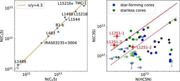
Figure 13. Left: the correlation between the column densities of C2S and C3S of low-mass cores quoted from the literature (Hirota et al. 2004; Hirota & Yamamoto 2006; Law et al. 2018; Agúndez et al. 2019; Nagy et al. 2019). Right: the correlation between the column densities of C3S (derived from C2S) and HC5N quoted from Suzuki et al. (1992), Hirota et al. (2009). The black filled squares represent sources detected in Wu et al. (2019a). The solid and dashed red lines represent y = x and y = x/3, respectively.
Download figure:
Standard image High-resolution image
Figure 14. The transitions of c-C3H2. The widths of the arrows represent the corresponding Einstein coefficients for spontaneous transition. Red arrows: observed transitions.
Download figure:
Standard image High-resolution imageThe right panel shows the correlation between the column densities of C3S (derived from C2S) and HC5N quoted from Suzuki et al. (1992), Hirota et al. (2009). All star-forming sources have N(C3S) lower than N(HC5N). There is only one formerly studied starless source, L1521E, having N(C3S) > N(HC5N). It seems impossible the cold gas components around young stars are responsible for the abnormally high abundance of C3S detected around YSOs in the L1251 region. Higher abundances of C3S compared to HC5N is a more strict criterion of SCCC in star-forming regions.
7. Summary
The previously identified SCCC sources all have N(C3S) > N(HC7N) but N(C3S) < N(HC5N) deduced from Ku-band observations (Wu et al. 2019a). We thus searched for SCCC sources, characterized by N(C3S) > N(HC5N), in the radio K-band (18–26 GHz) using the Effelsberg 100 m telescope. We identified L1251-1 as such a source and L1251-3 as a candidate. L1251-1 is located in L1251-A and harbors a Class Flat YSO (IRS1).
We further mapped L1251-A at the 3 mm band using the PMO 13.7 m telescope and the NRO 45 m telescope and in CO J = 3–2 using the JCMT. Combining the obtained spectra and archival data, including Spitzer and Herschel continuum maps, we investigated the morphology, environment, and dynamical characteristics of L1251-A as well as their relations to the phenomena of SCCC. The main results include:
- 1.Molecular lines of NH3, HC3N, HC5N, C3S, c-C3H2, and C4H were detected in three sources, L1251-1, L1251-2, and L1251-3. HFS and Gaussian fittings were applied to obtain basic parameters of the detected lines. Column densities and abundances of these detected species were calculated.
- 2.L1251-1 is characterized by N(C3S) exceeding N(HC5N) and is thus a confirmed SCCC source. L1251-3 has a C3S column density marginally larger than that of HC5N. L1251-1 has similar abundance ratios of N(C4H)/N(HC3N) and N(HC3N)/N(HC5N) to the SCCC sources in Wu et al. (2019a).
- 3.The volume densities of the three sources are constrained from the c-C3H2 11,0–10,1 emission line and the c-C3H2 22,0–21,1 absorption line based on the RADEX model with an ortho-to-para ratio of c-C3H2 assumed to be 3. We find the intensity ratio between c-C3H2 22,0–21,1 and c-C3H2 11,0–10,1 (noted as
 ) can serve as a volume density tracer. This method gives a volume density of 3 × 105 cm−3 for L1251-2, and the values for L1251-1 and L1251-3 are estimated to be ∼104 cm−3.
 - 4.The L1251 region consists of hierarchical filaments in Herschel continuum maps. Six sub-filaments labeled F1–F6 were extracted using FilFinder. F1 associated with L1251-A has two intertwined branches, the main branch (F1-M) and the side branch (F1-S). F1-S is about 0.4 km s−1 bluer than F1-M. Four YSOs (IRS1, IRS2, IRS3, and IRS4) are likely located on F1-M, although there is also possibility that IRS2 is on F1-S
- 5.The radial density distribution of F1 can be well fitted with a Plummer-like function. No large-scale velocity gradients, neither radially nor tangentially, are found in the main part of L1251-A
- 6.IRS3 and IRS4 (L1251-2) both show strong jets and outflows. A possible shocked region is found in the northwest of IRS4 and we name it IRS4-MNW. IRS4-MNW may be driven by the jet of IRS4. Outflow features are effective in this region and we speculate that there were outflows driven by IRS1 although extinguished now.
- 7.The interstellar medium around IRS1 and IRS3 has redder velocities than those around the other two YSOs (IRS1 and IRS2) and those on F1-S. The twisted spatial density distribution and velocity distribution along F1-M may present a large-scale MHD-transverse wave, resulting from outflows.
- 8.The emission of dense gas tracers such as HCO+ and N2H+ is associated with the main branch of F1 (F1-M). However, the emission of SO and C18O is much more enhanced in the eastern part of the side branch of F1 (F1-SE) compared to F1-M. Principal component analysis is applied and confirms this characteristic.
- 9.The peak positions of HCO+ clumps are misaligned with those of the dust clumps.
- 10.SCCC in L1251-1 may have been caused by outflow activities from the infrared source IRS1. L1251-1 (IRS1) together with the previously identified SCCC source L1251-IRS3 (Wu et al. 2019a) demonstrate that L1251-A is an excellent region to study SCCC.

Overall, the outflow activities in L1251-A are responsible for the physical characteristics, including the distorted velocity distribution along F1-M, the gas-dust misalignment, and the chemical property related to the abnormal high abundance of C3S.
This project was supported by the National Key R&D Program of China grant No. 2017YFA0402600, and the NSFC grant Nos. 12033005, 11988101, 11433008 11373009, 11503035, and 11573036.
D.M. acknowledges support from CONICYT project Basal AFB-170002. N.I. acknowledges PCI-ANID REDES190113. K.T. was supported by JSPS KAKENHI Grant Number 20H05645. K.W. acknowledges support by the National Key Research and Development Program of China (2017YFA0402702, 2019YFA0405100), the National Science Foundation of China (11973013, 11721303), and the starting grant at the Kavli Institute for Astronomy and Astrophysics, Peking University (7101502287).
We wish to thank the staff of the Effelsberg 100 m, NRO 45 m, PMO 13.7 m, and JCMT 15 m telescopes for their support during the observations. The Effelsberg 100 m telescope is operated by the Max-Planck-Institut für Radioastronomie (MPIfR). The Nobeyama Radio Observatory is a branch of the National Astronomical Observatory of Japan, National Institutes of Natural Sciences. The PMO 13.7 m telescope is operated by the Qinghai station of PMO at Delingha in China. The James Clerk Maxwell Telescope is operated by the East Asian Observatory on behalf of The National Astronomical Observatory of Japan; Academia Sinica Institute of Astronomy and Astrophysics; the Korea Astronomy and Space Science Institute; Center for Astronomical Mega-Science. Additional funding support is provided by the Science and Technology Facilities Council of the United Kingdom and participating universities in the United Kingdom and Canada.
This research has made use of the NASA/IPAC Infrared Science Archive, which is operated by the Jet Propulsion Laboratory, California Institute of Technology, under contract with the National Aeronautics and Space Administration.
Software: NOSTAR, FilFinder (Koch & Rosolowsky 2015), PySpecKit (Ginsburg & Mirocha 2011), RADEX (van der Tak et al. 2007), Starlink (Currie et al. 2014), GILDAS/CLASS.
Appendix A: YSO Classification
YSO classification based on the spectral index (αIR) in near- and mid-infrared bands defined as αIR = d(λ Lλ )/d λ was first proposed by Lada (1987), and followed and improved by works such as Wilking et al. (1989) and Greene et al. (1994). The four class system for low-mass YSOs based on αIR commonly used today can be described as

Andre et al. (1993) suggested a class "before" Class I named Class 0, and the YSOs located between Class 0 and Class I have protostellar masses similar to that of the remaining envelope. IRS1, IRS2, IRS3, and IRS4 have spectral indices of 0.19, 0.33, 0.70, and −0.52, respectively (Evans et al. 2009). Robitaille et al. (2006) found that YSOs with different spectral classes are distributed in different regions in the [3.6]–[5.8] versus [8.0]–[24] color–color diagram, and can also be used to classify YSOs. The four YSOs in the L1251-A region are all formerly located in the Class 0/I regions. IRS2 was reclassified by Dunham et al. (2013) from Class I to Class Flat through de-reddening it using an extinction value from the literature.
We fitted the SED of these four YSOs using the model of Robitaille (2017). Since our fitted sources, with the exception of IRS2, do not have data in 2MASS bands, the parameters of central stars and disks cannot be well constrained. The upper limits adopted as one-tenth the values of IRS2 are fed to the fitting procedures, instead. The distances are fixed at 300 pc, the V-band extinctions (AV ) are limited in the range of 0–50 mag, and the extinction law we adopted is the same as that used in Forbrich et al. (2010). The fitted luminosities of central stars (L⋆) of IRS1, IRS2, IRS3, and IRS4 are 0.3 L☉, 1.4 L☉, 1.1 L☉ and 0.25 L☉, respectively. If AV > 40 mag is permitted for IRS3 (Lee et al. 2010), corresponding to a deeply embedded YSO with a high accretion rate, the unobscured L⋆ can be much higher than the value listed here.
All arguments considered, the IRS3 is a Class 0/I object, IRS4 is classified as Class II, and IRS1 and IRS2 are classified as Class Flat.
Appendix B: Graybody SED Fitting
Pixel-by-pixel graybody SED fittings are applied to the Herschel archive data 33 covering the L1251 region in the 160, 250, 350, and 500 μm bands, observed by André et al. (2010) as part of the Herschel Gould Belt Survey. The Herschel 70 μm data were not used in our fittings, because of the limited S/N in this band. We first filtered out the background emissions of each map following Yuan et al. (2017), using the CUPID :FINDBACK algorithm of the Starlink suite. Then, we convolved each Herschel map with a Gaussian kernel with an FWHM of (in units of arcsec)

where θλ is the HPBW of the convolved Herschel map, and 35.2 (in arcsec) is the HPBW of the Herschel 500 μm map. The convolved maps were then re-gridded to obtain aligned images with a spatial pixel size 10'' × 10''. For each pixel, its corresponding intensities at different wavelengths in the range of 160–500 μm are fitted with a blackbody model,

where Bν is the Planck function, and the dust optical depth τν can be expressed as

Here, Σ is the surface density, and Rgd is the gas-to-dust ratio, which is assumed to be 100. The dust opacity κν can be expressed as a power law in the frequency of

The reference dust opacity at 600 GHz (500 μm) can be adopted as 5 cm2 g−1, the value for coagulated grains with thin ice mantles given by Ossenkopf & Henning (1994, hereafter OH5). In this work, κ(600 GHz) = 3.33 cm2 g−1 was adopted, which is scaled down by a factor of 1.5 from the OH5 value as suggested by Bianchi et al. (2003), Kauffmann et al. (2010). β is fixed at 2. There are two free parameters, the dust temperature Tdust and the surface density Σ to be obtained from the fitting procedures.
The uncertainty of the intensity at pixels (i,j) was taken as  , where
  was estimated as the rms value of regions free from emission, while
  was taken as 15% of the intensity of that pixel, based on the report by Launhardt et al. (2013). Only the pixels with intensities larger than 3σν;i,j
at all four bands were fitted by minimizing
was taken as 15% of the intensity of that pixel, based on the report by Launhardt et al. (2013). Only the pixels with intensities larger than 3σν;i,j
at all four bands were fitted by minimizing

The fitted maps of Tdust and Σ are shown in Figure 1.
The fitted pixels are enclosed by the black contour shown in the upper panel of Figure 1. The dust temperatures are as low as about 8 K in the central part of the fitted regions, and increase to about 12 K at the margins. For pixels outside the fitted regions, the dust temperatures are extrapolated by solving the Laplace's equation ∇2 T = 0, with the values of the fitted regions unchanged and the values of the pixels at the margins of the whole map fixed as 12 K. Numerically, ∇2 T = 0 can be solved by iterating

where  is the set consisting of the fitted pixels and the marginal pixels of the whole map. The surface densities for pixels outside the fitted regions are calculated based on the 500 μm intensities through Equations (B1) and (B3), and the extrapolated dust temperatures.
Appendix C: Calculated Column Densities
The column densities of molecules can be derived through (Wilson et al. 2009; Mangum & Shirley 2015)

where k is the Boltzmann constant, S is the line strength, μ is the dipole moment, and Qrot the partition function.
For NH3(1,1), the optical depth (τ), the intrinsic full-width at half-power line width (ΔVin), the LSR velocity (VLSR) and the amplitude  can be obtained through HFS fitting
  with
with

where where the ri are the relative intensities of the individual hyperfine lines in the optically thin case under conditions of thermodynamical equilibrium. The excitation temperature (Tex) can be obtained from

where Jν
(T) is defined by  , and Tbg is the background temperature.
For NH3, the equation to calculate the column densities of molecules in the (1,1) and (2,2) states can be expressed as

with ζ11 = 1.3850 × 10¹³ and ζ22 = 1.0375 × 10¹³ (Levshakov et al. 2013). Rotational temperatures ( ) can also be derived from the population ratio between the (2,2) and (1,1) states of NH3.
The rotational temperature  is adopted to calculate the total column density of NH3 (N(NH3)) assuming only the metastable states are effectively populated,

in which the ratio between the nuclear spin degeneracy (gI ) of para-NH3 (K ≠ 3n) and that of ortho-NH3 (K = 3n) is 2.
The volume density can be estimated for Tex ≠ Tkin through (Ho & Townes 1983; Levshakov et al. 2013)

where A is the Einstein A coefficient and C is the rate coefficient for collisional de-excitation.
Appendix D: Emission Model of c-C3H2
Figure 14 shows the energy diagram of c-C3H2. We calculated the intensities of the c-C3H2 11,0–10,1 and c-C3H2 22,0–21,1 lines produced in a uniform medium using the non-LTE radiative transfer code RADEX (van der Tak et al. 2007). The free parameters are the column density of para-C3H2 (Np
), the kinetic temperature (Tkin), as well as the densities of the collision partners. In our cases, H2 is taken as the only collision partner for both ortho-C3H2 and para-C3H2, and the background emission is fixed as 2.73 K. The space of the free input parameters (n(H2), Np
, Tkin) is gridded with n(H2) and N(X) evenly sampled on a log scale stepped by a factor of 3 from 103–107 cm−3 and from 1011–1015 cm−2, respectively, and Tkin evenly sampled from 5–30 K stepped by 1 K. For each set of input parameter, the integrated intensities (in units of Kelvin kilometers per second) of c-C3H2 11,0–10,1 ( ) and that of c-C3H2 22,0–21,1 (
 ) were calculated. Via extrapolation, the 3D surfaces
  (n(H2), Np
, Tkin) and
(n(H2), Np
, Tkin) and  (n(H2), No
, Tkin) can be obtained. Since the o/p ratios are fixed at 3, the flux ratio between c-C3H2 11,0–10,1 and 22,0–21,1 (
(n(H2), No
, Tkin) can be obtained. Since the o/p ratios are fixed at 3, the flux ratio between c-C3H2 11,0–10,1 and 22,0–21,1 ( ) can be expressed as

The two panels of Figure 15 show the relations between  and n with Tkin of 5, 14, and 23 K, and Np
at 1011 cm−2 (low column density case, hereafter LN) and 1013 cm−2 (moderate column density case, hereafter MN). In the LN case, all transitions are optically thin and
and n with Tkin of 5, 14, and 23 K, and Np
at 1011 cm−2 (low column density case, hereafter LN) and 1013 cm−2 (moderate column density case, hereafter MN). In the LN case, all transitions are optically thin and  increases monotonically with densities n(H2).
  is always larger than −0.45 in this case. In the MN case, the profiles of
  along n(H2) are similar to those in the LN case when n(H2) > 105 cm−3. However, when the density is low (n(H2) ∼103 cm−3), the absorption line 22,0–21,1 will be weak because the molecules are accumulated in lower energy states and the photons released from the 22,0−11,1 transition tend to be reabsorbed. In the MN case, if the volume density is low (nH2 ∼ 10 cm−3), the
  values are independent of kinetic temperature and always larger than −0.35. Compared with the LN case, another characteristic of the MN case is that
  will first slightly decrease as the density n(H2) increases.

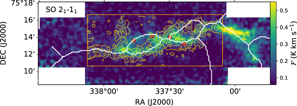
Figure 15. Upper panel: the dependence between  (flux ratio between c-C3H2 22,0–21,1 and c-C3H2 11,0–10,1) and n(H2) with the column density of para-C3H2 (Np
) fixed as 1012 cm−2. Lower panel: same as the upper panel except with Np
fixed as 1013 cm−2. The filled lines show the
(flux ratio between c-C3H2 22,0–21,1 and c-C3H2 11,0–10,1) and n(H2) with the column density of para-C3H2 (Np
) fixed as 1012 cm−2. Lower panel: same as the upper panel except with Np
fixed as 1013 cm−2. The filled lines show the  values. The dashed and dotted lines show the fluxes of c-C3H2 11,0–10,1 and c-C3H2 22,0–21,1, respectively.
Download figure:
Standard image High-resolution image
In the LN case with the kinetic temperature fixed at 10 K, the fitting between  and n(H2) gives

For  smaller than −0.35, the volume density should be smaller than or comparable with 104 cm−3, but cannot be well constrained. For
  larger than −0.35, the volume density should be larger than 104 cm−3. However, the assumption of the LN case may be not valid when the volume density is high, and Equation (D2) can only serve as a rough estimation of n(H2).
If the kinetic temperature is fixed and  is not too low (larger than −0.35), the free parameters n(H2) and Np
, as well as the optical depths, can be directly fitted from Equation (D1).
is not too low (larger than −0.35), the free parameters n(H2) and Np
, as well as the optical depths, can be directly fitted from Equation (D1).
Footnotes
- 22
- 23
- 24
The NRO is a branch of the National Astronomical Observatory of Japan, National Institutes of Natural Sciences.
- 25
- 26
- 27
- 28
- 29
- 30
- 31
- 32
- 33