


Abstract
The analysis of exoplanetary atmospheres often relies upon the observation of transit or eclipse events. While very powerful, these snapshots provide mainly one-dimensional information on the planet structure and do not easily allow precise latitude–longitude characterizations. The phase curve technique, which consists of measuring the planet emission throughout its entire orbit, can break this limitation and provide useful two-dimensional thermal and chemical constraints on the atmosphere. As of today, however, computing performances have limited our ability to perform unified retrieval studies on the full set of observed spectra from phase curve observations at the same time. Here, we present a new phase curve model that enables fast, unified retrieval capabilities. We apply our technique to the combined phase curve data from the Hubble and Spitzer space telescopes of the hot Jupiter WASP-43 b. We tested different scenarios and discussed the dependence of our solution on different assumptions in the model. Our more comprehensive approach suggests that multiple interpretations of this data set are possible, but our more complex model is consistent with the presence of thermal inversions and a metal-rich atmosphere, contrasting with previous data analyses, although this likely depends on the Spitzer data reduction. The detailed constraints extracted here demonstrate the importance of developing and understanding advanced phase curve techniques, which we believe will unlock access to a richer picture of exoplanet atmospheres.
Export citation and abstract BibTeX RIS
1. Introduction
In the field of transiting exoplanetary atmospheres, observational studies are dominated by two main techniques: transit and eclipse spectroscopy. The first consists of analyzing the changes in the wavelength-dependent transit depth when a planet passes in front of its host star while the second relies on observing the changes in the observed flux when the planet passes behind the star. These techniques are complementary, probing two distinct regions of the planet and being sensitive to different physical processes. Transmission spectra are most sensitive to the planetary radius, the cloud structure, and the atmospheric chemical species. Spectra from eclipse observations are sensitive to the combination of thermal changes with altitude and chemical abundances, making these observations particularly useful to study exoplanet thermal structures (Seager & Deming 2010; Tinetti et al. 2013; Madhusudhan 2019; Changeat & Edwards 2021). Most current retrieval codes extract information from such spectra using one-dimensional descriptions (Rodgers 2000; Irwin et al. 2008; Madhusudhan & Seager 2009; Line et al. 2013; Waldmann et al. 2015a, 2015b; Gandhi & Madhusudhan 2018; Al-Refaie et al. 2019; Mollière et al. 2019; Zhang et al. 2019; Edwards et al. 2020; Min et al. 2020). These models have been benchmarked, proving their consistency (Barstow et al. 2020) when the same assumptions are taken. In these models, the different processes can be modeled using free or self-consistent approaches. Self-consistent approaches attempt to reduce the number of free variables by modeling the physical phenomena from physicochemical principles. These can include, for example, solving the full radiative–convective equilibrium equations, including dis/equilibrium chemistry, two-stream temperature profile, or microphysical clouds. In contrast, a free approach does not assume much about the physical state of the considered system and uses parametric descriptions. As of today, there is no consensus on what should be adopted when analyzing real spectra and different assumptions can lead to different interpretations.
By design, transit and eclipse techniques offer the projection of a three-dimensional atmosphere to a one-dimensional spectrum with a wavelength dependence, from which it is difficult to extract the geometrical repartition of chemical and thermal properties (Feng et al. 2016; Line & Parmentier 2016; Caldas et al. 2019; Drummond et al. 2020; Feng et al. 2020; MacDonald et al. 2020; Pluriel et al. 2020b; Skaf et al. 2020; Taylor et al. 2020). To overcome these limitations and characterize the longitudinal structure of exoplanets, photometric and spectral phase curves have been used (e.g., Esteves et al. 2013; Placek et al. 2017; Deming & Knutson 2020; Parmentier & Crossfield 2018; Sing 2018; Barstow & Heng 2020). The technique consists of following the combined light (reflected and emitted) from the planet and star along the entire planet orbit, thus capturing the planet signal as a function of its phase. This technique is challenging, requiring a particularly high temporal stability, whereas current instruments limit its application to planets with short orbital periods. Only a handful of the known exoplanets have been observed in phase curves with the Hubble Space Telescope (HST), Spitzer, Kepler, and TESS (Parmentier & Crossfield 2018; Bell et al. 2021). Among those observations, HST provided particularly good constraints between 1.1 and 1.7 μm for WASP-43 b (Stevenson et al. 2014, 2017), WASP-103 b (Kreidberg et al. 2018), and WASP-18 b (Arcangeli et al. 2019). Spitzer obtained additional phase curve data at 3.6 and 4.5 μm for many planets, allowing to inform on circulation processes. Spitzer phase curve observations, for example, include 55 Cancri e (Demory et al. 2016), HD 209458b (Zellem et al. 2014), HD 189733b (Knutson et al. 2012), WASP-43 b (Stevenson et al. 2017), WASP-33 b (Zhang et al. 2018), HD 149026b (Zhang et al. 2018), WASP-12 b (Bell et al. 2019), and KELT-1 b (Beatty et al. 2019). Of these targets, WASP-43 b possesses the most complete set of observations, with high-quality spectra from both HST and Spitzer. The data were first analyzed in Stevenson et al. (2014, 2017), providing a unique insight into the properties of this world. Their spectral retrieval analysis was performed for each of the individual spectra obtained at each phase: in these analyses, no correlation between the different observed phases was considered. More recently, Irwin et al. (2020) used optimal estimation techniques to investigate the combined information content of the spectra at different phases. It was the first successful attempt to analyze the spectral phase curve of an exoplanet with a unified model. However, due to the computing cost of their model, concessions had to be made in the sampling technique. Their paper highlighted the limitations induced when using optimal estimation technique in exoplanet atmospheric studies, where observations have a low signal-to-noise ratio and the prior knowledge on the solution is unknown. Other studies highlighted the importance of using phase curve data to break the degeneracies coming from the three-dimensional aspect of exoplanets (Feng et al. 2016, 2020; Taylor et al. 2020). In particular, Feng et al. (2020) performed the first combined retrieval of the WASP-43 b phase curve using a full exploration of the parameter space with the MultiNest sampler (Feroz et al. 2009; Buchner et al. 2014).
In this paper, we propose an update of the forward model used in Changeat & Al-Refaie (2020) to compute the phase-dependent emission of tidally locked planets. Our semianalytical computation of atmospheric spectra enables Bayesian retrieval capabilities with full exploration of the parameter space. We applied the technique on the available WASP-43 b phase curve data from HST and Spitzer, showing the potential of phase curve techniques in extracting detailed three-dimensional atmospheric properties of exoplanet atmospheres and breaking degeneracies in transmission. We explore various model assumptions to investigate the information content of phase curve data and highlight model-dependent behaviors linked to these complex data sets.
2. Model Description
The analysis of the WASP-43 b phase curve spectra is performed using the Bayesian retrieval framework TauREx3 (Waldmann et al. 2015a, 2015b; Al-Refaie et al. 2019). Taking advantage of the new "plugin system" (A. F. Al-Refaie et al. 2020, in preparation), we developed a dedicated phase curve model enabling unified phase curve retrieval analysis. We updated the geometry presented in Changeat & Al-Refaie (2020) and built a phase-dependent model that is more adapted to calculate the emission of tidally locked planets. The planet is considered as a single entity, physically separated into three regions of similar properties (hot spot, day side, and night side). In tidally locked planets, the hot-spot region corresponds to the region of highest temperatures (the substellar point). The day side represents the remaining part of the day-side atmosphere, facing the star. The night side refers to the part in the atmosphere which does not receive direct stellar radiations. This separation is relevant for the study of irradiated tidally locked planets that are showing asymmetric emission and day–night contrasts in their observed phase curves, such as WASP-43 b (Stevenson et al. 2014, 2017). These features are potentially due to a directional redistribution of the atmosphere creating offsets in the observed brightness temperature (hot spot) and a cooler night side. In the three regions of our model, we consider that the chemistry, temperature, and cloud properties can be considered constant with latitude and longitude.
For each phase angle, the emission contribution of each region is calculated semianalytically via the computation of contribution coefficients: Ch i , Cd i , and Cn i , for, respectively, the hot spot, the day, and the night regions. For clarity, the details of the calculation of these coefficients are shown in Appendix A. By analyzing all the spectra together, the model ensures that the redundancy of the information content between the different spectra are taken into account. We also updated the transit model to account for the predicted strong differences in the day- and night-side atmospheres in these types of planets (Caldas et al. 2019; Pluriel et al. 2020b). The mathematical description of the new transmission model is detailed in Appendix B.
In the complete model (phase emissions + transmission), the calculation of the coefficients Ch i , Cd i , and Cn i is trivial for a computer and takes negligible time. In comparison to a standard emission or transmission model, we observe that this phase curve forward model is about five times slower. It can be understood by the fact that the complete model includes three emission models (one per region) and two transmission models (day and night-sides) for which the quantities (temperature, chemistry, clouds) and the optical depth must be computed (see Changeat & Al-Refaie 2020 for a more detailed discussion on the performances). We also highlight the fact that the most recent version of TauREx3.1 (A. F. Al-Refaie et al. 2020, in preparation) introduced the new plugin system, allowing the user to benefit from any other TauREx module without requiring a particular adaptation. As the phase curve model is based on the standard TauREx emission and transmission models, which have GPU accelerated plugins, our phase curve model is automatically compatible with GPU architectures.
3. Retrieval Setup
The hot Jupiter WASP-43 b was first reported in 2011 (Hellier et al. 2011) and, while its radius is similar to that of Jupiter, it is twice as massive (Hellier et al. 2011; Bonomo et al. 2017). It was immediately recognized as an extraordinary laboratory for atmospheric studies thanks to its very short orbit (0.8 days) and the data's particularly high signal-to-noise ratio. The entire phase has been observed with both Hubble and Spitzer, providing one of the most complete data sets to date. The complete phase curve was first analyzed in Stevenson et al. (2014, 2017), which unveiled variations in the chemical abundances of H2O, CO2, and CH4. They also revealed a particularly low emission from the planet night side, suggesting inefficient heat redistribution and/or a large cloud cover. We take WASP-43 b as an example for our phase curve investigation. We start by exploring the behavior of our technique on mock-up spectra for this planet (Section 4). Then, we analyze the phase curve data from the HST and Spitzer phase curve observations using a large range of retrieval scenarios (Section 5).
3.1. Observations
Real observations of WASP-43 b were used to test and illustrate the phase curve model presented in this paper. They were obtained from Stevenson et al. (2014, 2017) with no modifications. These consist of 15 already reduced spectra of the phase curve of WASP-43 b: 0.0625, 0.125, 0.1875, 0.25, 0.3125, 0.375, 0.4375, 0.5, 0.5625, 0.625, 0.6875, 0.75, 0.8125, 0.875, and 0.9375. The data were originally obtained by the Hubble Space Telescope in November 2013 (Program GO-13467) during three full orbital phases, three transits, and two eclipses with the WFC3 G141 grism (wavelength coverage from 1.1 to 1.6 μm). These consisted of spatially scanned images corresponding to 13–14 HST orbits for the phases and 4 HST orbits for the transit and eclipses. Complementary phase curve observations were obtained by the Spitzer Space Telescope, using the 3.6 μm (two visits, including one discarded) and 4.5 μm (one visit) photometric channels (Programs 10169 and 11001, PI: Kevin Stevenson). In addition to this, we also include the transmission spectrum from Kreidberg et al. (2014; in our model, this corresponds to phase 0.0) as this provides additional constraints on the day–night limb and allows us to extract the planetary radius with greater accuracy.
In emission, a large wavelength coverage is usually required to ensure that a sufficient pressure range of the atmosphere is probed, thus constraining the temperature structure (see Appendix D). Normally, this is done by combining the observations from HST and Spitzer to obtain spectra spanning 1.1–4.5 μm. The combination of instruments, however, can bring additional difficulties as nothing guarantees the compatibility of the observations. Sources of discrepancies can come from different instrument systematics, the use of different orbital elements, different reduction pipelines, and stellar or planet temporal variations (Yip et al. 2020, 2021; Changeat et al. 2020). As a consequence, independent studies of HST WFC3 data often lead to similar spectral shapes but different absolute depths (Changeat et al. 2020). Studies of the WASP-43 b Spitzer data (Stevenson et al. 2017; Mendonça et al. 2018a; Morello et al. 2019; Bell et al. 2021; May & Stevenson 2020) have also proved that independent reduction pipelines can obtain different results for the same Spitzer data set. In this paper, we use the Spitzer data from Stevenson et al. (2017) as is and do not investigate the potential implications of these effects. We however present a complementary retrieval in the Discussion section with the HST-only data, which highlights how the Spitzer points affect our solution. To date, this WASP-43 b data set is one of the most complete. Our integrated phase curve framework accumulates the information at all phases to extract extremely precise constraints on the atmospheric properties of this planet.
3.2. Opacity Sources
For this study, we assumed that the planet was mainly composed of hydrogen and helium with a ratio He/H2 = 0.17. We considered collision-induced absorption of the H2–H2 (Abel et al. 2011; Fletcher et al. 2018) and H2–He (Abel et al. 2012) pairs and included opacities induced by Rayleigh scattering (Cox 2015) and clouds. Because clouds are most constrained by the transmission spectrum, we model them with a fully opaque cloud layer above a given pressure, restricted to the day- and night-side regions. For the chemistry, we use the molecular line lists from the Exomol project (Tennyson et al. 2016, 2020; Chubb et al. 2021), HITEMP (Rothman & Gordon 2014), and HITRAN (Gordon et al. 2016). While many molecules are considered in the chemical equilibrium scheme, we only include molecular opacities for H2O (Barton et al. 2017; Polyansky et al. 2018), CH4 (Hill et al. 2013; Yurchenko & Tennyson 2014), CO (Li et al. 2015), CO2 (Rothman et al. 2010), C2H2 (Wilzewski et al. 2016), C2H4 (Mant et al. 2018), NH3 (Yurchenko et al. 2011), and HCN (Harris et al. 2006; Barber et al. 2013).
Table 1. List of the Parameters Fitted in the Retrieval, Their Uniform Prior Bounds, and The Scaling We Used
| Parameters | Prior Bounds | Scale |
|---|---|---|
| Metallicity | −1; 3 | log |
| C/O ratio | 0.1; 5 | linear |
| Free abundances | −12; −1 | log |
| Hot-spot temperature points (K) | 1000; 4000 | linear |
| Day temperature points (K) | 700; 3000 | linear |
| Night temperature points (K) | 300; 1700 | linear |
| Pclouds (Pa) | 7; 0 | log |
| Rp (Rjup) | 1; 1.1 | linear |
Note. Note that the parameters metallicity and C/O are activated for the equilibrium runs, while in the free chemistry run we use the free abundances parameters.
Download table as: ASCIITypeset image
3.3. Mock Retrieval Configuration
Section 4 aims to validate our method by presenting a retrieval on mock-up data where the true solution is known in advance. This approach allows us to check that our model is correctly implemented and will ensure that the results presented on real data, later on, are not artifacts of our method. This example is performed using Ariel simulated spectra, which also gives us the opportunity to investigate the Ariel capabilities to perform phase curve observations. The planet is simulated using the stellar and planet parameters from the literature (Bonomo et al. 2017). We first create the forward model at high resolution using our phase curve model with three distinct regions: hot spot, day side, and night side. Each region is composed of 100 layers spaced in log pressures. We assume homogeneous temperature profiles and a chemical compositions for the three regions inspired by previous works (Stevenson et al. 2014, 2017; Changeat & Al-Refaie 2020). For simplicity, the chemistry is modeled constant with altitude, and only H2O, CH4 and CO are included. In this example, the H2O abundance is set at 6 × 10⁻³ for the hot spot and 1 × 10⁻⁴ for the day and night sides. For CH4, the atmosphere contains 1 × 10⁻⁷, 1 × 10⁻⁵, and 1 × 10⁻⁴ for, respectively, the hot spot, the day side, and the night side. Finally, the CO abundance is set to 1 × 10⁻³ on the hot spot and 1 × 10⁻⁴ for the other regions. For this test, the hot-spot parameters were fixed to a hot-spot offset of 120 2, consistent with Stevenson et al. (2014), and a hot-spot size of 40°, matching findings from Kataria et al. (2015) and Irwin et al. (2020). This leads to 15 spectra from phase 0.0625 to phase 0.9375. We then bin down those spectra to Ariel observations assuming Tier 2 resolution and the observation of four complete planet revolutions. The noise was simulated using the Ariel Radiometric Model (ArielRad) from L. Mugnai et al. (2019, in preparation). We do not use random noise instances of our simulated observations for the retrievals, as we aim to study the retrieval biases arising from our retrieval technique (Feng et al. 2016; Changeat et al. 2019, 2020; Mai & Line 2019). Finally, we perform our phase curve retrieval test, leaving free the planetary radius, the temperature profiles, the constant chemical abundances, and the hot-spot parameters. The parameter space is explored uniformly with large bounds (see Table 1). The results of this exercise are described in Section 4.
3.4. Detailed Retrieval Configurations
Section 5 presents the results for the retrievals performed on the real data. Here, we consider the reduced observations described in Section 3.1. We also use the star parameters from Bonomo et al. (2017) and fix the planet mass (Changeat et al. 2020) to its radial velocity measurement (Bonomo et al. 2017). Because we always include the transmission spectrum in our retrievals, which is very sensitive to the planetary radius, we let this parameter as free. We note that complementary tests without including the transmission spectrum did not affect the results presented here. We performed an analysis of each spectrum individually (see Appendix C) and carried on with unified analyses using three classes of models of increasing complexity:
- Two-faces free: We considered a simplified geometry with no hot spot. We remove the influence from the hot-spot region by coupling all parameters (temperature, chemistry, clouds) between the hot-spot and the day-side regions. This allows us to check the consistency of our model and compare it with previous results from the literature. This setup uses a similar geometry to Feng et al. (2020). We considered free constant with altitude abundances for the molecules H2O, CH4, CO, CO2, and NH3. In the main scenario, these were coupled between all three regions. The free temperature profiles and cloud properties were left independent between the day and night regions. For the clouds, we use a simplistic fully opaque gray cloud. Two complementary runs were also used to explore the effect of the Guillot (2010) T–p profile and decoupled chemistry (different chemistry between the night and day sides).
(1) Two-faces equilibrium: For the second scenario, we used the same geometry but increased the complexity of our model by considering equilibrium chemistry for the day- and night-side regions. We used the scheme ACE from Agúndez et al. (2014). It calculates thermochemical equilibrium abundances for H-, He-, C-, O-, and N-bearing species, which is expected for hot Jupiters between 1000 and 2000 K. Only a fraction of the calculated molecules possess cross sections, so we limit the actively absorbing species to the ones described in Section 3.2. The chemistry was decoupled between the day and night regions (different chemical profiles) but the free parameters (metallicity and C/O ratio) are shared between all regions.
(2) Full: Finally, we performed simulations on the full model by introducing the hot-spot region described in Section 2. The definition of this region requires the additional hot-spot offset (Δ) and hot-spot size (α) parameters. In the first place, we attempted to retrieve these parameters but encountered inconsistencies with previous values from the literature (see posterior distribution in Appendix E). Because these degrees of freedom were already included in the reduction steps leading to the spectra (Stevenson et al. 2014, 2017), we decided to fix the hot-spot shift to the value in Stevenson et al. (2014): −122. For the hot-spot size, we tested the values 30°, 40°, and 50°, consistent with standard predictions from recent models for this planet (Kataria et al. 2015; Irwin et al. 2020) but only present the model with 40° in the result section. The complementary retrievals are presented in the discussion section and explore the impact of hot-spot size, hot-spot clouds, and the addition of the Spitzer data. We caution the fact that these apparent inconsistencies might be linked to incompatibilities of the spectra following the reduction process (this was not highlighted by our individual analysis in Appendix C), issues with our model assumptions (different planet geometry), or the lack of information content in the considered spectra.
In all scenarios, except when stated otherwise, the parameterization of the temperature profiles was done using the N-point profile from TauREx3 (Al-Refaie et al. 2019). This heuristic profile interpolates linearly between N freely moving temperature–pressure points. The profile is then smoothed over 10 layers to avoid inflection points. For the hot-spot and day regions, we retrieve seven temperature points at fixed pressures (106, 105, 104, 103, 102, 1, and 0.01 Pa). Because the information content decreases on the night side due to the lower emission, we found that retrieving five points (106, 105,103, 10, and 0.1 Pa) was more suitable. These choices are investigated in Appendix D, where various free temperature structures are explored. This level of complexity was chosen to maximize the Bayesian evidence in the retrievals of the WASP-43 b data from HST+Spitzer with the new phase curve model. We highlight, however, that other profiles lead to equivalent Bayesian evidence in the HST-only case.
The exploration of the parameter space is performed with uniform priors using the nested sampling algorithm MultiNest (Feroz et al. 2009; Buchner et al. 2014) with 500 live points and a log likelihood tolerance of 0.5. These choices ensure an optimal free sampling of the parameter space. All of the free parameters considered in this retrieval and their uniform priors are described in Table 1. The results of our investigation on the real data from WASP-43 b observations are presented in Section 5.
4. Mock Retrieval Results
The results of the retrieval on the ad hoc spectra are presented in Figure 1. The figure only shows the spectra for the phases from 0.0625 to 0.5, but the retrieval also included the phases from 0.5625 to 0.9375. As can be seen, the retrieval manages to produce a good fit of all the phases. The posterior distribution for the chemical species, displayed in the same figure, demonstrates that the retrieval is able to recover the correct abundances for water in all three regions. Methane is recovered on the day side and the night side, but the molecule is not captured on the hot spot, which has a lower input abundance of 10−7. CO, which is present with high abundance on the hot spot and the day side was only retrieved from the day side. CO possesses a single broadband feature in the Ariel wavelength range (Changeat et al. 2020) and is therefore more challenging to constrain. This lower signature, associated with the higher input abundance of H2O and the smaller size of the hot spot as compared to the rest of the day side, could explain the difficulties of our retrieval to constrain this molecule on the hot spot. We note that the hot-spot offset is properly recovered with very high accuracy, which indicates the theoretical capabilities of this class of models to directly constrain the geometrical properties of exoplanet atmospheres. For the temperature structure, the retrieval recovers the noninverted thermal profiles with very good agreement (see Figure 1). We did not observe discrepant behavior in this retrieval, validating the capabilities of our model for retrieval applications. This example also shows the potential of the Ariel Space Telescope for phase curve retrieval studies. Ariel is expected to yield spectra for about 1000 exoplanets in transit and eclipse mainly; however, a significant amount of observing time will be dedicated for phase curves studies as part of the Tier 4 survey (Tinetti et al. 2018; Edwards et al. 2019a).

Figure 1. Results of our retrieval on the WASP-43 b simulated spectra as observed with Ariel. Top: observed and best-fit spectra from phase 0.0625 to 0.5. The observed data points are randomly scattered in this figure for visual were not randomly scattered for the retrieval. Bottom: posterior distributions (left) and Temperature structure inferred by our retrieval. The solid lines correspond to the true values. Red: hot spot; orange: day side; blue: night side.
Download figure:
Standard image High-resolution image5. Real Data Results
In this section, we present the results from our unified retrievals on the real phase curve spectra obtained from Stevenson et al. (2014, 2017). The retrieval setups we use are described in Section 3.4. For comparison, we complement this exploration with a more standard approach, applying our model to the individual spectra in Appendix C. We also provide some exploratory work on the required complexity when considering free temperature profiles in Appendix D. The best-fit spectra, obtained for each scenario, are compared in Appendix F.
5.1. On Model Comparison
For an easier comparison of our results, we provide the model integrated values in the Spitzer bands and the χ2 values corresponding to each spectrum. We note that χ2 values on individual spectra might be difficult to interpret for model comparison in a Bayesian context and should be viewed with caution (Edwards et al. 1963). In particular, the data set and parameters considered in this work are not expected to be independent, while the tested models are also nonlinear (Andrae et al. 2010; Gelman 2013). The stated χ2 value is calculated for the best-fit model, which might not be representative of the larger pool of solutions found via our Bayesian inference technique. Within a Bayesian framework, the Bayesian evidence, log(E), is used for model comparison and accounts for both goodness of fit and model complexity (Rougier & Priebe 2020). When comparing two models, a log difference of 3 indicates a strong preference for the model with the highest evidence (Kass & Raftery 1995; Jeffreys 1998). When testing models of increasing complexity, their Bayesian evidence should also increase as long as the additional flexibility is justified. For models of adequate complexity, the Bayesian evidence should plateau around a maximum value. Finally, if the model overfits, the Bayesian evidence should decrease.
5.2. Two Faces Free: Benchmark Retrieval
In this run (log(E) = 2238.1), we consider only two regions: day and night sides. The geometry and the chemistry model (free chemistry) are similar to what has recently been presented in Feng et al. (2020), which allows us an easier comparison with their findings. A major difference in our model is the parameterization of the temperature structure. Here, we choose a free temperature profile, and we retrieve the temperature structure from the day and night side independently. Indeed, alternative physics-based descriptions, such as the parameterization from Guillot (2010), assume a one-dimensional atmosphere experiencing irradiation from two sources (upward and downward fluxes). While this describes well a planet day side with poor atmospheric redistribution, this geometry does not accurately represent the night side of a tidally locked planet, which are by definition not receiving direct stellar flux. For all models in this paper, except when stated otherwise, we therefore opted for a free parameterization. The best-fit spectra, the geometry, and the posteriors for our two-faces free chemistry model are described in Appendix G (blue runs). These highlight the difficulty of the model to fit the Spitzer points around the secondary eclipse. This is most likely due to the symmetry enforced in this type of geometry. The temperature profile for the day side mainly decreases with altitude, which is consistent with previous studies (Stevenson et al. 2014, 2017; Kataria et al. 2015; Irwin et al. 2020; Feng et al. 2020), but we note the preference (large 1σ uncertainties) for a thermal inversion above 103 Pa. We ran complementary retrievals, parameterizing the temperature profile with the prescription from Guillot (2010), and found a noninverted temperature profile and chemistry (orange runs in Appendix G), similar to the findings in Feng et al. (2020). This run, however, led to a particularly low Bayesian evidence of log(E) = 2045.2, potentially highlighting the lack of flexibility in the Guillot profile. We discuss the presence of thermal inversions for this planet later, in the section describing the results of the Full model scenario. On the night side, the temperature is poorly constrained due to the low flux received at these phases. We note that the model prefers high-altitude clouds. In terms of chemical species, this retrieval finds very constrained abundances for water and ammonia (see posteriors). These match the abundances found by the joint scenario in Feng et al. (2020). As opposed to their results, the free T–p profile run does not recover constraints on CO2, which can be explained by our use of the more flexible temperature structure. Indeed, when the Guillot profile was used, we recovered a similar abundance for CO2 (see orange posteriors in Appendix G). This retrieval exploration using the two-faces free chemistry model confirms the findings presented in Stevenson et al. (2017), Irwin et al. (2020), and Feng et al. (2020), and also highlights different solutions when using more flexible temperature structures (also see Appendix D). We also ran a complementary retrieval where the chemistry is decoupled between the day and night sides. This retrieval led to two solutions corresponding to the green (log(E) = 2242.3) and gray (log(E) = 2240.4) runs in Appendix G. Because the gray run corresponds to an unphysically high mean molecular weight solution, we focus on the green solution. Due to the large day/night temperature contrast, differences in the chemistry can be expected. This retrieval presents a very different chemistry from the previous models with a much higher water content on the day side (around 10−2) and a much more complex temperature structure. The chemistry recovered here is similar to the ones presented in the next sections using decoupled equilibrium chemistry models (two-faces equilibrium and full models). On the night side, we do not recover any molecules.
5.3. Two Faces Equilibrium: Equilibrium Chemistry Retrieval
One major assumption, taken in the previous scenario, is the constant chemistry with altitude and longitude. Previous studies showed that atmospheric chemistry is not constant and that assuming so could lead to observable biases (Venot et al. 2012, 2020; Agúndez et al. 2014; Drummond et al. 2018; Stock et al. 2018; Woitke et al. 2018; Changeat et al. 2020; Drummond et al. 2020). In order to provide a more realistic description of chemical properties, one could either assume more complex parameterizations (Parmentier & Crossfield 2018; Changeat et al. 2019) or use self-consistent chemical models (Agúndez et al. 2014; Stock et al. 2018; Woitke et al. 2018). While both approaches are viable with high-quality data, the low wavelength coverage of HST favors the more constrained models. We therefore assumed equilibrium chemistry for all three regions using the scheme from Agúndez et al. (2014). Because we assume that atomic elements are evenly spread across the planet atmosphere, this leaves us with only two free parameters: metallicity and C/O ratio. The impacts of these assumptions are explored more in the Discussion section. We present the best-fit spectra, chemical profiles, temperature structure, and posteriors in Appendix H. As compared with the previous run, the use of equilibrium chemistry allows us to better fit the Spitzer photometric points (log(E) = 2245.8). In this scenario, the retrieved chemistry is well constrained (see posterior distribution). The atmosphere is consistent with a slightly supersolar metallicity ( ) and a low C/O ratio (
 ). In particular, the use of the chemical scheme allows large variations in the abundances of carbon-bearing species between the day and night side. There are linked to the large retrieved temperature differences between the two regions (from 2500 K down to 500 K) and are matching the findings in our free chemistry run with decoupled chemistry (green run in Appendix G). As compared to the two-faces free run, an interesting difference is the retrieved abundance for water. Here, we find that the abundance for water remains constant between the two regions (as expected from thermochemical equilibrium) but that it might be two orders of magnitude higher than the values found in the free chemistry case (log(H2O) = −4.4). In fact, we find that a very similar solution (with high water abundance) can also be recovered from a free chemistry retrieval when the abundances between the day and night-side regions are decoupled, clearly indicating the need to account for chemical variations between those two regions. In terms of temperature structure, we find a day-side temperature profile that mainly decreases with altitude and the presence of a thermosphere, similar to the free chemistry run. The night side is much colder and includes high-altitude clouds at pressures as high as 10 Pa.
5.4. Full Retrieval
The previous models have difficulties fitting the spectra for the phases near eclipse. This is due to the symmetry imposed when considering only two faces. To increase the complexity, we split the geometry into three distinct regions: hot spot, day side, and night side. For the run presented here, the model has a fixed hot-spot size of 40°. We also model the planet without including clouds on the hot spot (the cloud-top pressure was fixed at 106 Pa). This choice is justified by theoretical predictions, which suggest that the hot day side of irradiated exoplanets might be cleared due to the strong stellar irradiation (Lee et al. 2016; Parmentier et al. 2016; Lines et al. 2018; Helling 2019). The best-fit spectra for this scenario and the corresponding geometries are shown in Figure 2. For this retrieval, we obtain a log evidence of 2277.4, which indicates the relevance of adding this additional region to the model.

Figure 2. Best-fit spectra and geometry of our WASP-43 b phase curve retrieval with the full model. At the top, we show the eclipse (left) and the transit (right). Green diamonds represent the average Spitzer bandpasses. The right panels have an inverted wavelength axis.
Download figure:
Standard image High-resolution imageWe also investigated the same run on the HST spectra only. Both HST+Spitzer and HST-only runs are presented in Appendix I, which provides a zoomed version of the same run around the HST wavelength range. The HST+Spitzer run is colored while the HST-only run is gray. Both fits (with and without the Spitzer photometric points) do not show major differences in the HST wavelength range and are well fitted to the observed data. Outside the HST wavelength coverage, however, we see that the inclusion of the Spitzer points leads to large differences in the retrievals.
The temperature structure associated with the HST+Spitzer retrieval is presented in Figure 3, which as expected, clearly displays a hotter day side and a more strongly irradiated hot spot.
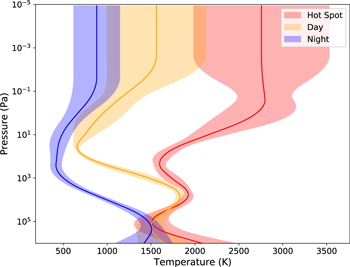
Figure 3. Retrieved mean and 1σ temperature structure of WASP-43 b for the different regions. Hot spot: red; day side: orange; night side: blue. The hot spot presents a significantly higher temperature, especially at the top of the atmosphere.
Download figure:
Standard image High-resolution imageAs in the free temperature two-faces runs presented in previous sections, the temperature structure is consistent with the presence of thermal inversions for this planet. This contrasts with previous findings from Blecic et al. (2014), Stevenson et al. (2014), and Kreidberg et al. (2014). The retrieved temperature structure indicates the presence of a stratosphere (above 105 Pa) and the presence of a thermosphere (above 10 Pa) on the planet's day side and hot spot. We note that the current data do not allow us to probe the highest altitude (thermosphere) with great accuracy, leading to large 1σ uncertainties on the retrieved profile (around ±600 K). This is also shown in the contribution functions for each region, which are plotted in Appendix J. In the full model and for most of the temperature structures explored in Appendix D, the hot spot and day side present a thermal inversion at high altitudes, below 1 Pa. This drives the thermal dissociation of all molecules at those altitudes, making the atmosphere transparent. We discuss further the interplay between this high-altitude thermal inversion and our chemical model assumptions in the discussion section. For this planet, thermal inversions are predicted (Showman et al. 2009; Kataria et al. 2015) in the presence of optical absorbers such as atomic species (K, Na) or metal hydrides and oxides (e.g., AlO, FeH, SiO, TiO, TiH, or VO). The presence of aluminum oxide (AlO) in the transmission spectrum of WASP-43 b has recently been highlighted in Chubb et al. (2020). This detection, made at the terminator region, is not expected from equilibrium chemistry models at the temperatures and pressures considered (Chubb et al. 2020; Helling et al. 2020). Chubb et al. (2020) highlighted that the presence of this molecule could come from disequilibrium or dynamical processes. The higher temperature on the day side allows for this molecule and other metal oxides/hydrides in a gaseous form (Woitke et al. 2018), which could then be transported to the terminator regions (Caldas et al. 2019; Pluriel et al. 2020b). Earlier ground-based observations of the transit (Chen et al. 2014) were also consistent with optical absorption, which were interpreted as pure Rayleigh scattering or absorption from K/Na or TiO/VO. Their observations of the eclipse suggested poor day–night contrast, as also suggested in our results, and potential high-altitude emission on the planet day side.
From a theoretical perspective, recent studies have also shown that thermal inversions could occur naturally in the upper atmosphere of hot Jupiters (Lothringer et al. 2018; Lavvas & Arfaux 2021). For example, the day side of irradiated hot Jupiters might be significantly heated by photochemical hazes and/or dissociation of the main molecules and the addition of continuum opacity from negative hydrogen (H–). In addition, local thermal inversions are also predicted to occur if sulfur-bearing species are present (Lavvas & Arfaux 2021). While the investigations in Lothringer et al. (2018) were performed on an F-type star with a larger UV flux than WASP-43 (K-type), their fiducial hot-Jupiter simulations showed that planets at distances from their host star similar to WASP-43 b (0.1 au) and with equilibrium temperatures around 1500 K could display inversions above 100 Pa, regardless of their TiO/VO content. The results presented here might provide strong observational evidence in favor of these theoretical predictions.
In Figure 4, we also show the atmospheric structure derived from our model. The planet presents an inflated day side (and hot spot) with a large-scale height difference between the day and the night regions. This conclusion also holds for the models with only two faces, strongly suggesting that using one-dimensional transmission models to analyze transit spectra might lead to large biases for these types of planets as their current formulations lack the flexibility to properly represent such three-dimensional effects. A recent study (Skaf et al. 2020) already found observational evidence of these effects in Hubble transmission spectra and, as next-generation telescopes will be more and more precise, this indicates the importance of considering complementary phase curve studies. For irradiated targets, phase curves will bring additional constraints that will allow us to break these three-dimensional degeneracies. On the night side, we retrieve a large temperature decrease with altitude, which can be inferred from the very low emission of the spectra at these phases. Similar results were already highlighted in Stevenson et al. (2014, 2017), Irwin et al. (2020), and Feng et al. (2020).
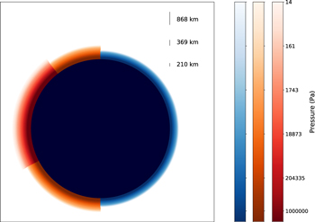
Figure 4. Retrieved atmospheric structure of WASP-43 b. The red region is the hot spot (shifted by 122); the orange region is the day side; the blue region is the night side. The legend corresponds to the altitude at 5 scale heights. We notice that the hotter temperatures on the day side lead to a significantly larger atmosphere.
Download figure:
Standard image High-resolution imageThe abundance profiles predicted by our equilibrium chemistry scheme for this planet are shown in Figure 5. The retrieved metallicity ( ) and C/O ratio (
 ) for this atmosphere, shown in the posterior distribution in Appendix K, are particularly well constrained. These correspond to a slightly carbon-enriched atmosphere with a supersolar metallicity, which contrasts with the previous two-faces equilibrium retrieval. For WASP-43 b, global climate models (GCMs) have shown that supersolar metallicities provide a better fit to the Stevenson et al. (2017) data (Kataria et al. 2015). Their work, however, explored lower metallicities than considered in our study. They also highlighted that the presence of night-side clouds provides a good explanation of the observed data. Overall, we find that water remains present in all regions of the atmosphere and that its abundance is consistent with our previous two-faces equilibrium run. Carbon is converted from mainly CO on the day side to CH4 on the night side, with an overall higher abundance of these species compared with the previous runs. We note that NH3, which will be a very strong absorber in the spectra from the next-generation telescopes, such as JWST (Greene et al. 2016), Twinkle (Edwards et al. 2019b), and Ariel (Tinetti et al. 2018), might reach detectable abundances on the night side of the planet.

Figure 5. Molecular abundances in the different regions according to the chemical equilibrium scheme. Red: hot spot; orange: day side; blue: night side.
Download figure:
Standard image High-resolution imageIn terms of cloud properties, our full scenario did not recover evidence of opaque absorbing layers on the night side. Although clouds have been suggested as an explanation for the very low temperature of the night side, we highlight the fact that all spectra, even at low orbital phases, are showing some prominent water absorption features at 1.4 μm, which explains why clear atmosphere solutions are favored when enough flexibility is given to the model. While we did not detect direct evidence of night-side clouds, these are not ruled out, and because the signal on the night-side phases is lower, the retrieval does not inform us about clouds at pressures higher than 104 Pa.
Overall, when compared to our previous runs without a hot spot and/or the results from Stevenson et al. (2017), Irwin et al. (2020), Feng et al. (2020), we obtain a very different picture. When a hot spot is added, our retrieval finds that thermal inversions (stratosphere and thermosphere) with a rich chemistry provides the best fit to the combined phase curve spectra.
5.5. Section Summary
In the three scenarios dealing with real data, we recovered particularly well-constrained solutions. By considering all spectra together, the information content contained in our analysis is increased as compared to traditional single-spectrum retrievals. This can be seen by comparing the results to our phase curve retrievals on individual spectra (see Appendices C and D) and the results from this section with our unified exploration. This allows us to extract more complex information as compared to previous studies. In all three cases, we recover a decent fit of the spectra. This is showcased in Appendix F, where we compare the best-fit spectra of our three scenarios. We note the increase in complexity between the different scenarios allows us to better reflect the observed data, as shown by the increase in log(E), especially in the Spitzer region. For example, the inclusion of the hot spot with a shift of −122 in the Full model improved the capability to fit the slightly higher flux observed from phases 0.0625–0.4375 (See also Figure 2). This is expected as the raw phase curve data from WASP-43 b exhibit day–night contrast and asymmetric emission, features that require a minimum of three regions to be properly described. Interesting different interpretations of the data can be made from the solutions recovered by our three scenarios.
More precisely, our two-faces free chemistry retrieval indicates similar results to previous studies for this planet (Stevenson et al. 2017; Feng et al. 2020), but it also highlights the need for increased complexity, matching the information content in the spectra. We find a hot day side with a large temperature decrease and a cool night side. The retrieved chemistry is also fairly similar, with a relatively low abundance of water. When we introduce variations with altitude and longitude in the chemistry (two-faces model with equilibrium chemistry), the retrieval prefers models with higher water abundances (two orders of magnitude larger). This behavior drives a supersolar metallicity and C/O ratio. In our most complex scenario, when a hot spot is added, the temperature profile displays a stratosphere with a thermal inversion around 103 Pa on the day side and hot spot. This is associated with a different chemistry with a supersolar metallicity and a slightly higher C/O ratio. The solution also appears stable to changes in the model parameters such as clouds and hot-spot size. In all three scenarios, the best-fit T–p profiles on the day side are consistent with a thermosphere, a high-altitude thermal inversion. In essence, these tests demonstrate the potential of phase curve data in describing three-dimensional effects and the feasibility of extracting this information using retrieval frameworks. This also clearly shows the model dependence of data analysis techniques and the need to use models of adapted complexity.
6. Discussion
In our retrieval with a hot spot, a large number of assumptions were made: hot-spot size, clear hot spot, the addition of the Spitzer data, and other model assumptions such as chemistry or temperature parameterization. As all retrieval analyses are to some degree model dependent, it is always interesting to study the stability of a solution to model assumptions, especially because large differences are observed in the model without a hot spot. In this section, we present complementary runs and illustrate caveats that are relevant to understand the stability of our solution.
6.1. The Impact of the Hot-spot Size
When performing the retrievals with free hot-spot size and offsets, we encounter solutions that do not match the values recovered in Stevenson et al. (2014, 2017), motivating the need to fix those two values (see Appendix E). While there might be observational reasons to fix the hot-spot offset (we use the peak emission in the phase from Stevenson et al. 2014), the hot-spot size cannot be constrained easily from prior analyses. For our baseline run, it was set to 40° following suggestions from three-dimensional studies (Kataria et al. 2015; Irwin et al. 2020; Helling et al. 2020) but other values might, in fact, also explain the observed data. The impact of the hot-spot size can be investigated by running complementary retrievals with various hot-spot sizes. We considered the cases with 30° and 50° fixed hot-spot sizes. For the chemistry and the clouds (see Appendix K), comparisons of the three simulations indicate very similar results. The temperature structure also remains similar in most of the atmosphere, but there are a few differences in the top part of the hot spot and the day side where the retrieved temperature increases with a smaller hot spot. As only little differences appear, it explains the difficulties in recovering reliable information on the geometry of this planet with current data. Using similar techniques to the one presented in this paper, we however believe that data from the next-generation telescopes, with a larger wavelength coverage and a higher signal-to-noise ratio, might be sensitive enough to infer the hot-spot geometry directly. Section 4 provides an example where the hot-spot shift is directly captured in the retrieval of Ariel data.
6.2. Model with Hot-spot Clouds
In our baseline model, we represented the planet without including clouds on the hot spot (the cloud-top pressure was fixed to 106 Pa). This choice is justified by theoretical predictions from Lee et al. (2016), Parmentier et al. (2016), Lines et al. (2018), and Helling (2019), which suggests that the hot day side of irradiated exoplanets might be cleared up due to strong stellar irradiation from the host stars.
When clouds are included on the hot spot, we recovered a clear hot-spot solution, but the posterior solution also includes a cloudy hot-spot scenario with clouds up to 103 Pa (see Appendix L). As a result, the corresponding temperature profile in the cloudy hot-spot solution presents larger uncertainties for higher pressures, which are in this case enabling a wider range of solutions without necessarily stratospheric thermal inversions. While opaque clouds are less likely present on the day side of WASP-43 b, recent theoretical models of this planet from Helling et al. (2020) suggest that this region could host some mineral clouds with a large particle size as well as photochemically driven hydrocarbon hazes. With a much stronger day-side emission, the information contained in the phase curve data is greater for these regions, thus potentially allowing us to detect the first pieces of evidence confirming these predictions.
6.3. Importance of the Spitzer Data for This Analysis
It is known that combining data from multiple instruments can lead to strong degeneracies (Yip et al. 2020, 2021; Irwin et al. 2020; Changeat et al. 2020; Feng et al. 2020; Pluriel et al. 2020a) in retrieval results. While we believe the use of HST along with Spitzer provides a large wavelength coverage, necessary to simultaneously infer atmospheric properties in emission spectroscopy (temperature/clouds/chemistry), the stability of the solution is investigated by reproducing our retrieval on the HST data only. Appendix I provides the spectra centered around the HST wavelength range for our HST+Spitzer retrieval (colored spectra) and our HST-only case (gray). The runs are also extended to the Spitzer region in Figure 29 of Appendix I. Neither fit (with and without the Spitzer photometric points) shows major differences in the HST wavelength range and is well fitted to the observed data. Outside the HST wavelength coverage, however, we see that the inclusion of the Spitzer points is leading to large differences in the retrieval predictions.
For the thermal structure, we found similar results (see Appendix I), with larger errors on the retrieved profiles for the HST-only run. This behavior is expected from the decrease in information content because HST only covers a short wavelength range. The addition of the Spitzer data leads to observational constraints on the carbon-bearing species: CH4 at 3.6 μm; CO and CO2 at 4.5 μm. The chemistry, in the HST-only case, pushed toward very high metallicities (log(m) > 2.0 for the posterior distribution in Appendix I). We believe the addition of the Spitzer points is required to simultaneously retrieve the temperature and chemistry profiles in emission. The addition of the 3.6 and 4.5 μm Spitzer points provide valuable information to constrain the carbon-bearing species, thus impacting the retrieved chemistry greatly. We highlight, however, that the Spitzer data points are sensitive to the reduction employed. For the particular case of WASP-43 b, there are now five independent studies (Stevenson et al. 2017; Mendonça et al. 2018a; Morello et al. 2019; Bell et al. 2021; May & Stevenson 2020) that obtained very different reductions, potentially introducing biases to our results. In addition, most models use simple sine functions to reduce phase-curve data, and alternative physically motivated approaches might provide different results (Louden & Kreidberg2018).
6.4. Other Model Choices
In this work, we assumed a particular geometry when computing the phase curve emission. The solutions found with this new model contrast with previous analyses (Stevenson et al. 2017; Irwin et al. 2020; Feng et al. 2020) and highlight new possibilities for the atmosphere of WASP-43 b. The choices made here aimed to achieve a balance between our current understanding of the physical properties of irradiated planets and the complexity of the analyzed data. However, as of today, there is no obvious way to assess the amount of information that can be extracted from an exoplanet spectrum or a set of spectra. For example, we demonstrated that the analysis of phase curve data with unified phase curve models allows for the extraction of a more complete and complex picture than standard techniques. However, there is no guarantee that our model is complex enough or best represents the planet's geometry. In other terms, when fitting exoplanet data, one always recovers a model-dependent solution and in our case, other three-dimensional geometries might be more accurate or relevant than what we presented. In the case of phase curves, we believe complementary work (testing more complex/simple geometries, comparing with simulated data) must be performed to completely understand the model-dependent errors introduced by our choices. We highlight, however, that the technique presented in this work is very general and can be adapted to other three-dimensional geometries. We intend to evolve this model to reflect the advancements in our understanding of three-dimensional effects.
Similarly, this comment also applies to physical and chemical assumptions, which might lead to biases, too. In our most complex run, we assumed the planet chemistry is in thermochemical equilibrium and that the chemistry is coupled between the different regions. While suggested as a good approximation for hot-Jupiter planets in the temperature ranges of WASP-43 b, this may not be the case and previous studies already demonstrated the dangers of assuming equilibrium chemistry for exoplanets undergoing disequilibrium processes (Line & Yung 2013; Rocchetto et al. 2016; Mendonça et al. 2018b; Blumenthal et al. 2018; Changeat et al. 2019; A. F. Al-Refaie et al. 2020, in preparation; Changeat et al. 2020; Steinrueck et al. 2019; Drummond et al. 2020; Venot et al. 2020). In particular, the thermal inversion observed in the full model for pressures lower than 1 Pa is driven by the need to increase the temperature and thermally dissociate all the molecules, which makes the atmosphere transparent there. In fact, if other mechanisms are able to remove the molecules at those altitudes, the retrieval would most likely not require such strong thermal inversions, which we believe is linked to the equilibrium chemistry assumption. Such processes could, for example, come from photodissociation. In addition to this, the current equilibrium scheme we use does not include exotic molecules such as TiO, VO, AlO, or H–. This might also lead to biases and have an important impact on the predicted molecular abundances, especially as the results from this analysis suggests the presence of thermal inversions on the day side of this planet. The definitive detection of such optical absorbers would provide further evidence to verify the thermal inversion hypothesis. Similarly, clouds were assumed as fully opaque gray opacities, which is a simplification that will have to be challenged when considering higher-quality spectra from next-generation telescopes (Bohren & Huffman 2008; Heng & Demory 2013; Lee et al. 2013; Powell et al. 2018, 2019; Barstow 2020; Helling et al. 2020). For WASP-43\,b, reflected light, which is not included here, is shown to have an important impact on the energy budget of this planet (Keating & Cowan 2017). Finally, our exploration of the parameter space was performed using the MultiNest routine (Feroz et al. 2009), which is well established in the exoplanet community. However, the recovered solutions might also depend on the sampling algorithms used, for example, alternative nested sampling algorithms are described in Handley et al. (2015), Speagle (2020), and Buchner (2021); the chosen settings; and the convergence criteria. We tested our full scenario with an increased number of live points (2500) to verify the stability of our solution to this parameter. The posterior distribution, shown in Appendix M, does not indicate different results compared to the 500 live points run for this example, but we note that retrieval abilities to separate multimodal solutions might greatly depend on this parameter.
7. Conclusion
Phase curve data associated with a unified analysis such as the one presented in this paper, undeniably provide a more complete picture of exoplanet atmospheres than conventional methods. By using a new type of simplified representation for the exoplanet WASP-43 b, we demonstrated the feasibility of building dedicated techniques for the study of these complex data sets. This technique provides access to an unprecedented level of detail, which, along with the upcoming increase in data quality by next-generation space-based instruments, has the potential to revolutionize our understanding of exoplanet atmospheric physics. However, by testing different assumptions for the geometry, the chemistry, and the thermal structure of WASP-43 b in our model, we demonstrated the impact of model assumptions on the result recovered (see summary in Table 2). With the upcoming JWST and Ariel next-generation space telescopes, this highlights the importance of studying these model-dependent behaviors to ensure the optimal extraction of higher-quality spectral data.
Table 2. Assumptions and Main Results from the WASP-43 b Retrieval Runs Presented in this Paper (C: Coupled; DC: Decoupled; eq: Equilibrium; HS: Hot Spot)
| N | Retrievals | Assumptions | Highlighted results | log(E) | Sections |
|---|---|---|---|---|---|
| 1 | Two-faces free T–p (C) | C free chemistry | Low H2O abundance and NH3 consistent with the literature | 2238.1 | 5.2 |
| DC free T–p | Mostly noninverted T–p with a potential thermal inversion | ||||
| DC gray clouds | Night-side clouds | ||||
| 2 | Two-faces Guillot T–p (C) | C free chemistry | Low H2O abundance, CO2, and NH3 consistent with Feng et al. (2020) | 2045.2 | 5.2 |
| DC Guillot T–p | Noninverted T–p consistent with Feng et al. (2020) | ||||
| DC gray clouds | No clouds—these were not included in Feng et al. (2020) | ||||
| 3 | Two-faces free T–p (DC) | DC free chemistry | High H2O, CH4, and CO2 abundances (not consistent with 1 and 2) | 2242.3 | 5.2 |
| DC free T–p | Presence of a stratosphere | ||||
| DC gray clouds | High-altitude night-side clouds | ||||
| 4 | Two-faces equilibrium | C eq chemistry | High abundances for H2O, CH4, CO, and CO2 (similar to retrieval 3) | 2245.8 | 5.3 |
| DC free T–p | Mostly decreasing, presence of a thermosphere | ||||
| DC gray clouds | Day- and night-side clouds | ||||
| 5 | Full 40° | C eq chemistry | Supersolar metallicity | 2277.4 | 5.4 |
| DC free T–p | Presence of stratosphere and thermosphere on the day side | ||||
| DC but clear HS | No clouds | ||||
| 6 | Full (other HS sizes) | C eq chemistry | Supersolar metallicity (very slight changes from 5) | 2278.2 | 6.1 |
| DC free T–p | Same as 40°, with a T–p increase for smaller HS | ||||
| DC but clear HS | No changes in clouds from 5 | ||||
| 7 | Full 40° (HS clouds) | C eq chemistry | Supersolar metallicity (same as 5) | 2277.3 | 6.2 |
| DC free T–p | Presence of stratosphere and thermosphere on the day side | ||||
| DC allowed on HS | No clouds on day and night sides but possible on HS | ||||
| 8 | Full 40° (HST only) | C eq chemistry | Very high metallicity (nonphysical) | 2101.6 | 6.3 |
| DC free T–p | Presence of thermosphere. Larger T–p uncertainties than in 5 | ||||
| DC but clear HS | No clouds on day and night sides | ||||
Download table as: ASCIITypeset image
We thank the referee for providing thoughtful suggestions that greatly improved our manuscript.
This project has received funding from the European Research Council (ERC) under the European Union's Horizon 2020 research and innovation program (grant agreement No 758892, ExoAI) and under the European Union's Seventh Framework Programme (FP7/2007-2013)/ERC grant agreement numbers 617119 (ExoLights). Furthermore, we acknowledge funding by the Science and Technology Funding Council (STFC) grants: ST/K502406/1, ST/P000282/1, ST/P002153/1, ST/S002634/1, and ST/T001836/1.
This work utilized the OzSTAR national facility at Swinburne University of Technology. The OzSTAR program receives funding in part from the Astronomy National Collaborative Research Infrastructure Strategy (NCRIS) allocation provided by the Australian Government. This work utilized the Cambridge Service for Data Driven Discovery (CSD3), part of which is operated by the University of Cambridge Research Computing on behalf of the STFC DiRAC HPC Facility (www.dirac.ac.uk). The DiRAC component of CSD3 was funded by BEIS capital funding via STFC capital grants ST/P002307/1 and ST/R002452/1 and STFC operations grant ST/R00689X/1. DiRAC is part of the National e-Infrastructure.
Data Availability
The data analyzed in this work are available through the NASA MAST HST archive (https://archive.stsci.edu/) programs 13665 and 14682. The molecular line lists used are available from the ExoMol website (www.exomol.com).
Appendix A: The Phase-dependent Emission Model
The phase-dependent emission model uses the principles developed in Changeat & Al-Refaie (2020). The new geometry accounts for high day–night temperature contrasts and the presence of a hot spot by simulating the planet using three separated homogeneous regions: hot spot, day side, and night side (see Figure 6).

Figure 6. Diagram of the phase curve geometry used in this paper. We show the three regions in shaded colors. Red: hot spot; orange: day side; blue: night side. The labels in green correspond to three-dimensional angles emerging from the center of the planet sphere. The red labels are two-dimensional projections in the (y, z) plane, which is perpendicular to the line of sight (tangent to the celestial sphere). The blue circle corresponds to the two-dimensional Gaussian quadrature integration circles, also projected onto the celestial sphere plane. Φ is the phase angle considered, Δ parameterizes the hot-spot offset, and α defines the size of the hot-spot region. The integration circle is defined by its viewing angle μ = cos(θ). The coordinates of Ph and Pn , the points of intersection with the integration circle, are the quantities to determine.
Download figure:
Standard image High-resolution imageFor each region, the angle-dependent specific intensity at the top of the atmosphere is given by

where μ is the viewing angle, Tsurf is the surface temperature, τ is the optical depth (labeled with surf for the surface and 0 for the top of the atmosphere), and B is the Plank function (Waldmann et al. 2015a). The integral over τ is performed over Nlayers layers equally spaced in logarithmic pressure.
To obtain the total specific intensity, Equation (A1) must be integrated over μ. This step is numerically done using the Gaussian quadrature integration technique, which consists of integrating the planet emission over NG integration circles at discretized viewing angles μi . In the standard emission case, the total specific intensity at the top of the atmosphere is given by

where ωi are the quadrature weights.
In the case of a planet with regions and a phase-dependent emission additional weight coefficients can be introduced to account for the contribution of each region to each Gaussian quadrature term in the final emission. Thus, Equation (A2) becomes
where Φ is the phase angle considered.  ,
,  , and
, and  are the day, terminator, and night intensities at the top of the atmosphere for the Gaussian point μi
. For each phase considered and for a given geometry, the C coefficients (hot spot: Ch
; day side: Cd
; night side Cn
) allow us to map the weight of each region to each Gaussian quadrature integration circle. The total number of Gaussian quadrature points is labeled NG
.
are the day, terminator, and night intensities at the top of the atmosphere for the Gaussian point μi
. For each phase considered and for a given geometry, the C coefficients (hot spot: Ch
; day side: Cd
; night side Cn
) allow us to map the weight of each region to each Gaussian quadrature integration circle. The total number of Gaussian quadrature points is labeled NG
.
Because the coefficients C are phase dependent, Equation (A3) gives the specific intensity for a given phase angle Φ. When another phase angle is evaluated,  ,
,  , and
, and  do not need to be recomputed and only the values of the C coefficients, which have been precomputed, are updated.
These coefficients correspond to the intersections between the Gaussian quadrature integration circles and the different region boundaries (we note those Ph and Pn in Figure 6). The specific intensity of each region is calculated using the base emission model from TauREx 3 (Al-Refaie et al. 2019). The coefficients are projected onto the planet plane (orthogonal to the line of sight). In 3D, the hot-spot and terminator boundaries are considered circles on the surface of the planet sphere. These are therefore described by intersections between planes (defined by the chosen hot-spot and terminator positions) and the sphere (for the planet). In addition to this, the Gaussian integration circles are equivalent in 3D to cylinders of circular bases and directions parallel to the line of sight. In Cartesian coordinates (x, y, z) with x pointing toward the observer, the problem is therefore equivalent to solving the following set of equations:
- 1.Region plane : Ax + By + Cz + D = 0.
- 2.Planet sphere: x2 + y2 + z2 − 1 = 0.
- 3.Gaussian integration cylinder: y2 + z2 − 1 + μ2 = 0.
Solving these equations for (x, y, z) leads to four possible solutions for the point of intersection Pint that can be formulated using Expression (A4):
The coefficients A, B, C, and D define the plane equation, hence the position of the hot-spot and the terminator boundaries. These are defined as a function of θ the inclination angle (assumed equal to 0 in this study), Φ the phase angle, Δ the hot-spot shift, and α the hot-spot size angle and are unique to each phase angle. Their expressions are summarized in Table 3.
Table 3. List of the A, B, C, and D Coefficients Depending on the Boundary Considered (Hot Spot and Terminator) for Equation (A4)
| Coefficient | Hot-spot Boundary | Terminator |
|---|---|---|
| A | cos(θ) cos(Φ − Δ) | cos(−θ) cos(Φ − π) |
| B | cos(θ) sin(Φ − Δ) | cos(−θ) sin(Φ − π) |
| C | sin(θ) | sin(−θ) |
| D | cos(α) | cos(π/2) |
Download table as: ASCIITypeset image
Finally, the coefficients Ch and Cn can be calculated from Equation (A4) as the angles from the y axis to the intersection points Ph and Pn . For a point of intersection Pint of coordinates (yint, zint), the angle is given by

The last coefficient is calculated using the remaining difference:

These equations can be used immediately in most cases. However, some particular situations, corresponding to the cases of ill definitions of Equation (A4), need to be accounted for individually:
- 1.When the integration circle is fully inside a region R, the intersection coefficients Ch i and Cn i do not exist. Then the corresponding coefficient CR i = 1 and the two other ones are 0.
- 2.If only one coefficient CR i exist, then the integration circle is shared with only 2 regions and the other coefficient is equal to 1–CR i .
Finally, the observed planet-specific intensity can be computed for each phase using Equation (A3). The observed flux ratio ΔΦ at a phase Φ is then computed using

where Rp is the planetary radius, Is the stellar intensity, and Rs is the radius of the star.
Appendix B: Transmission Model
The transmission model considers that the stellar light is filtered through both the day side and night side. This consideration accounts for the 3D effects explored in Caldas et al. (2019), Pluriel et al. (2020b), where large day–night temperature contrasts on tidally locked irradiated exoplanets create sudden geometrical changes at the planet limb. In their work, they highlighted that the more traditional assumption of 1D atmosphere leads to strong biases in the retrieved transmission spectra. In order to account for these effects, we assumed that the atmosphere can be described by two contributing regions (the day and night sides in our model). For this study, the light rays seen in transit are therefore filtered through the day-side region for half of their path and through the night-side region for the other half. Retrievals from Irwin et al. (2020), Stevenson et al. (2014, 2017), and the 3D GCM from Kataria et al. (2015) have shown that the planet WASP-43 b presents a large day–night contrast, thus confirming the relevance of this treatment. In practice, we compute both day and night properties and combine them using

where A is the atmosphere contribution, τ1 is the optical depth along the line of sight of the day side, and τ2 is the one from the night side.
The final transit depth Δ∣ is calculated by

This description allows us to account for day- and night-side properties seen in transmission. The transmission spectrum therefore provides some constraints linking both hemispheres. For planets where only the transmission spectrum is observed, it might be difficult to break the degeneracies arising from three-dimensional effects at the limb. In a full phase curve analysis, however, the day side is informed from the various emission models and properties, meaning that the degeneracy is diminished and that the night-side and terminator properties can be inferred from the residual information in the transmission spectrum.
Appendix C: Retrievals on Individual Phases
We explore the information content of each phase by running our phase curve retrieval model separately for each spectrum. This way, we assess whether our combined phase curve retrieval strategy allows us to extract more information from this data set. To avoid biases, we use free parametric models for both chemistry (constant with altitude) and temperature descriptions (NPoint profile described in the Method section). The molecules considered are H2O, CH4, CO, and NH3, and clouds are added to the day and night sides. The retrieved thermal profiles, chemical abundances, and cloud-top pressures are presented in Figure 7.
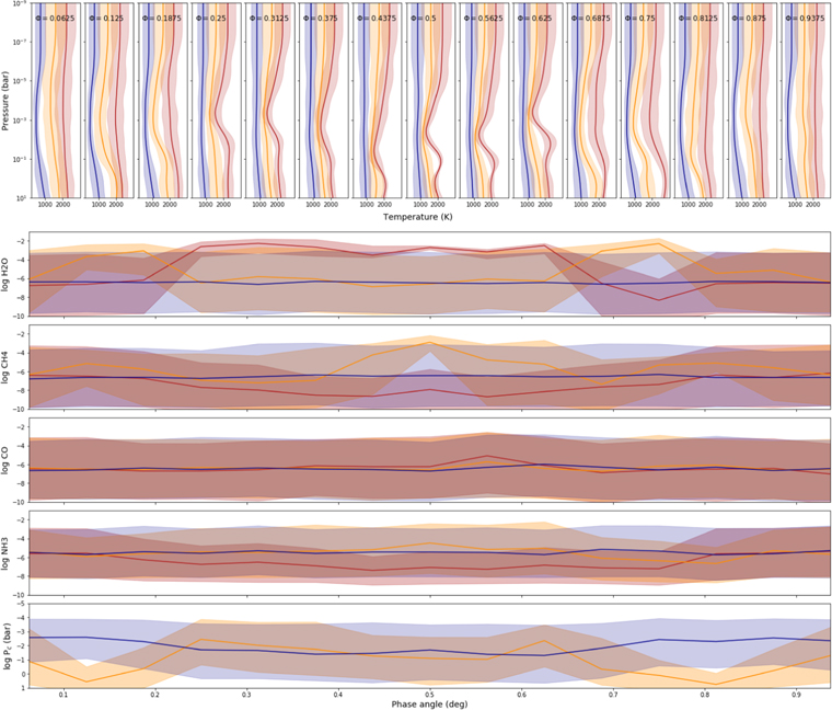
Figure 7. Temperature profiles (top) and retrieved chemical/clouds values (bottom) as a function of phase for the individual spectra retrievals. The temperature profiles and retrieved chemistry are aligned for phase angles between the top and bottom panels.
Download figure:
Standard image High-resolution imageFor the temperature profile, the expected behavior is observed. We see that the observations close to the transit are not constraining the day-side and hot-spot profiles but tighten the constraints on the night-side profile, while the observations closer to the eclipse give more information regarding the day-side and hot-spot temperature structure. For most of the profiles, the temperatures are decreasing with altitude, but we note that some phases around 0.5 show a weak thermal inversion at the hot spot. The retrieved chemistry indicates the presence of water vapor in both the hot spot (dominant for phases between 0.25 and 0.625) and the day side (dominant outside). Interestingly, methane is only detected at the day side in one spectrum (phase 0.5), which is surprising and might indicate remaining systematic errors in this spectrum. Additional constraints on other molecules and the night-side region remain poor due to the low contribution of this region. For the clouds, these are not detected in either the day side and the night side, but stronger constraints can be obtained for the day side at intermediate phases due to the greater flux. Overall, our phase curve retrievals on the individual spectra provide indications that two-dimensional effects can already be captured in emission spectra from HST (eclipses or phase curves) because the model was successfully able to separate the chemical and temperature structures for all three considered regions. This result was already discussed in previous work by Taylor et al. (2020) and Feng et al. (2020), where the possible biases of using simpler one-dimensional retrieval models are explored. The extraction of a consistent picture between these different retrievals, which are not considering the spectra together, provides us with indications that the whole data set might be consistent and adapted for our unified retrieval exploration.
Appendix D: Retrieval Exploration of Various Free Temperature–Pressure Models
Here, we explore the required complexity when using free thermal profiles to extract information from HST and Spitzer spectra. The results of this appendix can serve as a rough guideline but are only relevant for the considered WASP-43 b data set as other planet spectra might have significantly different information content. In the first place, we evaluate the required complexity for a single phase, using 1D retrievals of the day-side spectrum. This exercise is done with and without the Spitzer data to show the benefits of adding a larger wavelength coverage. Then we perform a unified phase curve exploration. For each case, we evaluate four different models. The first three models have three, four, and five temperature–pressure nodes, and for each point, we attempt to retrieve both temperature and pressure. Because including more fully free points dramatically increases the required number of samples (above 10 million) to reach an accurate sampling of the parameter space, the last model includes seven temperature points at fixed pressures (106, 105,104, 103, 102, 1, and 0.01 Pa). For a low number of nodes (<5), retrieving both pressure and temperature is required as fixing a particular node pressure would be arbitrary. When a larger number of nodes (>5) is used, fixing the pressure has fewer consequences as all regions of the atmosphere are well sampled. We note that the number of free parameters of the different models is, respectively, five, seven, nine, and seven, meaning that the four-point profile and the seven-point profile with fixed pressure nodes have the same number of parameters. As those profiles present different characteristics, it might be difficult to define the absolute concept of "complexity." For this exploration, we assume chemical equilibrium in all models and only retrieve the metallicity and C/O ratios.
(1) 1D retrievals on the day-side HST spectrum
The retrievals assuming different temperature–pressure structures on the HST-only data set are presented in Figures 8 and 9. The different scenarios lead to very similar log(E): 121.1, 121.2, 122.2, and 120.7 for, respectively, the three-point, the four-point, the five-point, and the seven-point profiles with fixed pressure for the nodes. These values are all within a small range and because the Bayesian evidence naturally penalizes for model complexity, it indicates that all the tested models are good candidates to explain the data. Taking a conservative approach, we however favor the simplest model that best explains the data (Occams razor principle), which is the three-point temperature profile. We note, however, that all models of higher complexity present some hints of thermal inversions in the upper atmosphere with large uncertainties.
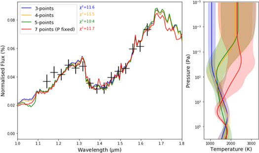
Figure 8. Retrieved spectra (left) and temperature profiles (right) of different 1D retrievals when assuming different free temperature–pressure profiles. The data points are for phase 0.5 of the HST data.
Download figure:
Standard image High-resolution image(2) 1D retrievals on the day-side HST+Spitzer spectrum
When considering the HST+Spitzer data, we find a similar conclusion (see Figures 9 and 10). All of the models are within the same range of log(E) with values of, respectively, 134.0, 133.9, 132.1, and 133.6 for the tested models. Again, this does not allow to conclude on a particular model, but a conservative approach would be to select the "simplest model": three-point model.
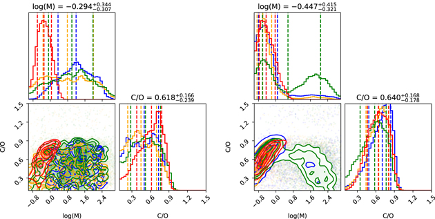
Figure 9. Posterior distributions of the 1D retrievals on phase 0.5 when assuming different free temperature–pressure profiles. The color scheme is the same as in Figure 8. Left: HST only; right: HST+Spitzer.
Download figure:
Standard image High-resolution image
Figure 10. Retrieved spectra (left) and temperature profiles (right) of different 1D retrievals when assuming different free temperature–pressure profiles. The data points are for phase 0.5 of the HST+Spitzer data.
Download figure:
Standard image High-resolution image(3) Unified phase curve retrievals on HST only
The same exercise was also repeated with the phase curve model to assess the required complexity for the thermal profiles. Because the emission of each region is capture by multiple spectra, one can expect the information content of each region to increase as compared to an individual spectrum retrieval. When performing the unified retrievals on HST data, the five-point temperature profiles required many model evaluations (>15 million) to reach the imposed convergence criteria (evidence tolerance of 0.5). We therefore choose to fix the pressure points for those profiles as is done for the seven-point profile. We however explored two choices for the fixed pressure points of the five-point model that were informed by the results of the seven-point model. In the five-point (informed) scenario, we fixed the pressure points to 106, 105, 100, 1, and 0.01 Pa. This setup allows us to follow the solution found when using seven points. In the five-point (no inversion), we attempt to remove the inversion seen around 104 Pa by setting the 5 pressure points to 106, 105, 104, 100, and 0.01 Pa. The results of those retrievals are shown in Figures 11–13. The three-point profile obtained log(E) = 2100.2, the four-point profile obtained log(E) = 2102.4, the five-point (informed) profile obtained log(E) = 2103.9, the five-point (no inversion) profile obtained log(E) = 2100.0, and the seven-point profile with the fixed pressure node obtained log(E) = 2101.6. While a slight preference can be seen for the five-point (informed) model, all the tested models obtained evidence that are roughly in the same range, making the choice of a particular model difficult. We note that all temperature profiles, except the simplest, exhibit a thermal inversion at high altitude. When testing the different five-point models, we obtained a noticeable difference in the log evidence (ΔE = 3.7 for the informed model). This difference highlights that fixing the pressure points of a free thermal profile can lead to user-dependent behaviors when a small number of nodes is used. In all models, we find a supersolar metallicity, and depending on the model, the C/O ratio can be subsolar to solar.
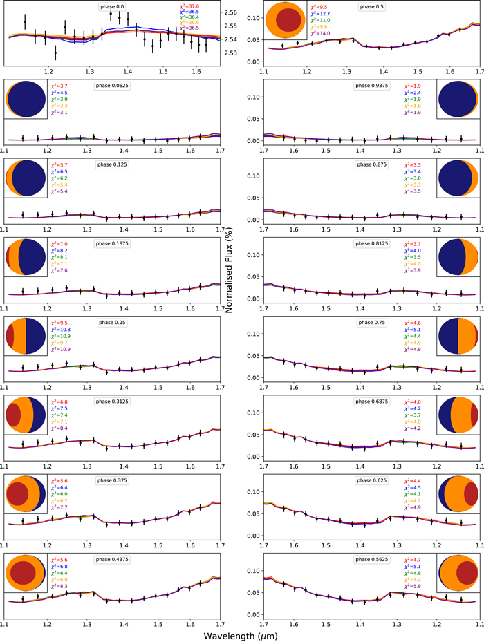
Figure 11. Retrieved spectra from unified retrievals on the HST data when assuming different free temperature–pressure profiles. Blue: three-point; green: four-point; orange: five-point (informed); purple: five-point (no inversion); red: seven-point (fixed P) profiles.
Download figure:
Standard image High-resolution image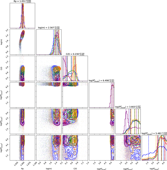
Figure 12. Posteriors from unified retrievals on the HST data when assuming different free temperature–pressure profiles. Blue: three-point; green: four-point; orange: five-point (informed); purple: five-point (no inversion); red: seven-point (fixed P) profiles.
Download figure:
Standard image High-resolution image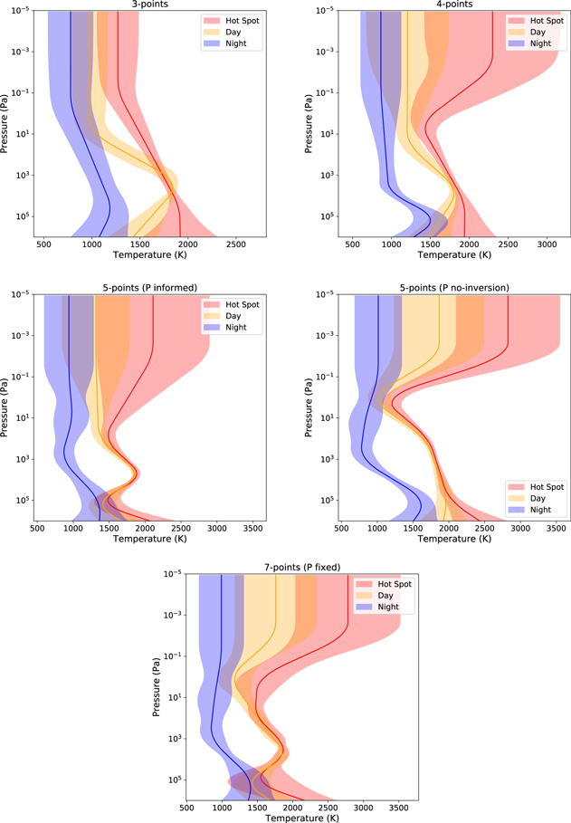
Figure 13. Retrieved temperature profiles from unified retrievals on the HST data when assuming different free temperature–pressure profiles. Note that the pressure of the temperature nodes is fixed for the five-point and seven-point scenarios.
Download figure:
Standard image High-resolution image(4) Unified phase curve retrievals on HST+Spitzer
This time, we find that a more complex structure is required (see Figures 14–16). The three-point profile obtained log(E) = 2267.2, the four-point profile obtained log(E) = 2275.0, the five-point (informed) profile obtained log(E) = 2278.0, the five-point (no inversion) profile obtained log(E) = 2272.6, and the seven-point profile with the fixed pressure node obtained log(E) = 2277.4. The significant difference in evidence between the simplest and the most complex models indicates that additional information is brought by the Spitzer data. In fact, thermal profile shapes similar to those in HST-only runs are found, but with tighter constraints. For all runs, the metallicity is again supersolar, while the C/O ratio is subsolar to solar depending on the thermal profile considered. Now, having determined that a complex thermal profile is required to best extract the information contained in the WASP-43 b phase curve data, we choose to use the seven-point profile as our baseline in this article. This is motivated by performance reasons (retrieving pressure has proven to require many more samples) and to avoid user-dependent behavior as shown with the five-point profile.

Figure 14. Retrieved spectra from unified retrievals on the HST+Spitzer data when assuming different free temperature–pressure profiles. Blue: three-point; green: four-point; orange: five-point (informed); purple: five-point (no inversion); red: seven-point (fixed P) profiles.
Download figure:
Standard image High-resolution image
Figure 15. Posteriors from unified retrievals on the HST+Spitzer data when assuming different free temperature–pressure profiles. Blue: three-point; green: four-point; orange: five-point (informed); purple: five-point (no inversion); red: seven-point (fixed P) profiles.
Download figure:
Standard image High-resolution image
Figure 16. Retrieved temperature profiles from unified retrievals on the HST+Spitzer data when assuming different free temperature–pressure profiles. Note that the pressure of the temperature nodes is fixed for the five-point and seven-point scenarios.
Download figure:
Standard image High-resolution imageIn this exercise, we only explored scenarios of various complexities for the thermal profile. The complexity of a model should match the information content in the data but ensuring this is by no mean easy in the context of exoplanet atmospheres because retrievals often include many modules dealing with different parts of the physics. For example, in case of a bad fit, should one increase the complexity of the thermal profile or the chemistry? This question is difficult to answer and will essentially always lead to user-dependent choices. Here, our chemistry is kept relatively simple for practical reasons, but it is not inconceivable that a more complex chemistry or the addition of new absorbers would lead to different results.
Appendix E: Retrieval with the Free Hot-spot Offset
In Figure 17, we show the posterior distribution of the "Full" retrieval run, leaving the hot-spot offset as a free parameter. The recovered parameter does not match the Stevenson et al. (2014) value of 122. In all the other runs of this paper, we fix the hot-spot value to 122, but we note that the conclusions from the free hot-spot shift run are the same as the full run.
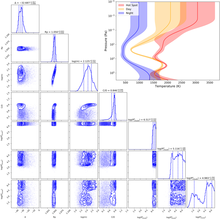
Figure 17. Posterior distribution and temperature structure (top right) of the full retrieval scenario with the free hot-spot offset parameter.
Download figure:
Standard image High-resolution imageAppendix F: Best-fit Spectra of the Two-faces Free, the Two-faces Equilibrium, and the Full Retrievals
We show in Figures 18 and 19 the best-fit spectra and geometry of our 2-faces free, 2-faces equilibrium and full retrievals.
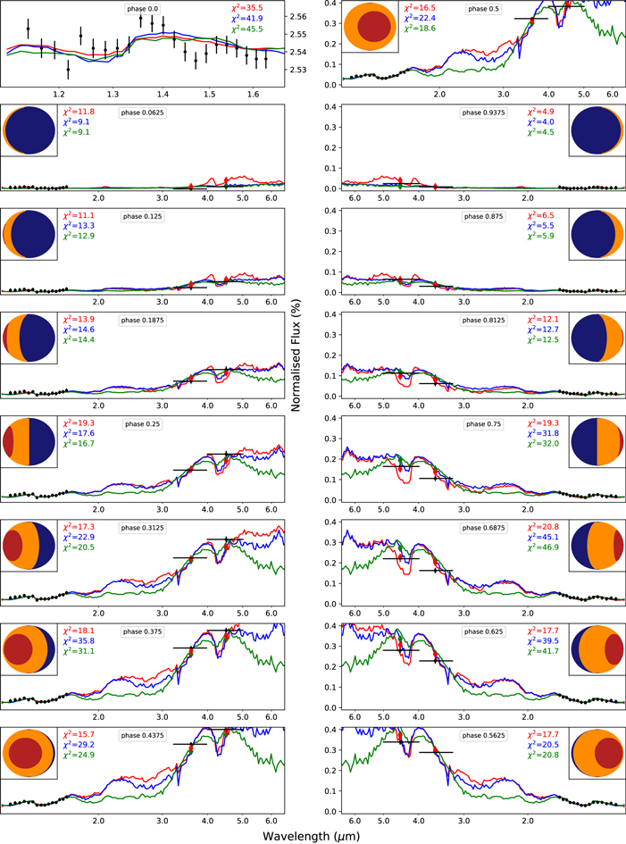
Figure 18. Best-fit spectra and geometry of our WASP-43 b phase curve retrieval with the two-faces free chemistry model (green), the two-faces equilibrium chemistry model (blue), and the full model (red). The diamonds represent the averaged Spitzer bandpasses. The right panels have an inverted wavelength axis.
Download figure:
Standard image High-resolution image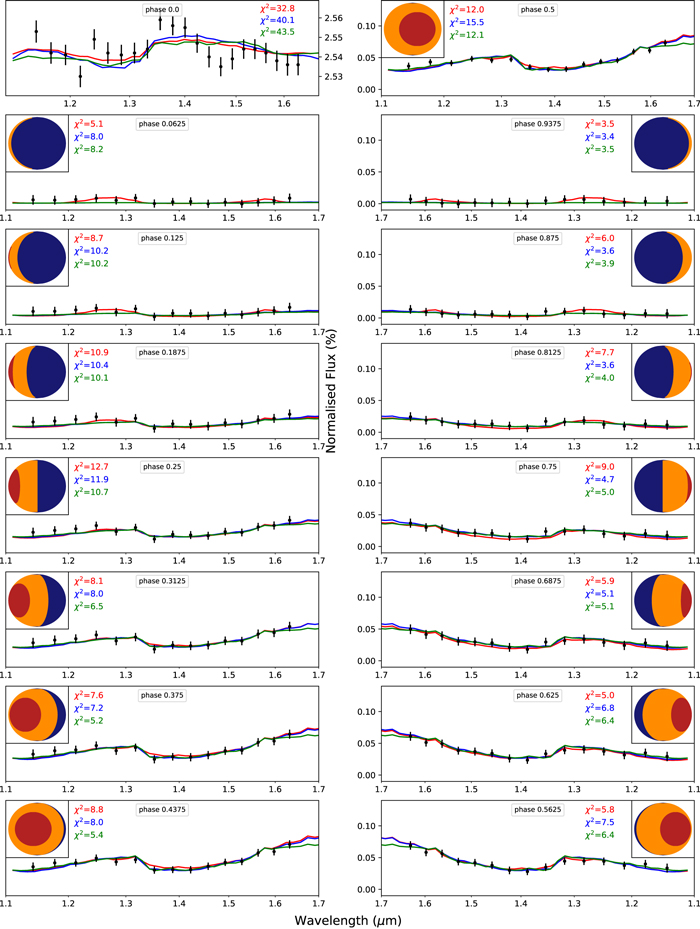
Figure 19. Best-fit spectra and geometry of our WASP-43 b phase curve retrieval with the two-faces free chemistry model (green), the two-faces equilibrium chemistry model (blue), and the full model (red). It is the same as Figure 18 but zoomed in the HST wavelength range. The right panels have an inverted wavelength axis. The χ2 was calculated for the data between 1.1 and 1.7 μm only.
Download figure:
Standard image High-resolution imageAppendix G: Complementary Plots of the Two-faces Free Chemistry Retrieval
Figure 20 shows the best-fit spectra and geometry in our 2-faces free chemistry retrieval. Figure 21 compares the thermal structure recovered for different assumptions in our 2-faces free scenarios. Corresponding posterior distributions are shown in Figures 22 and 23.
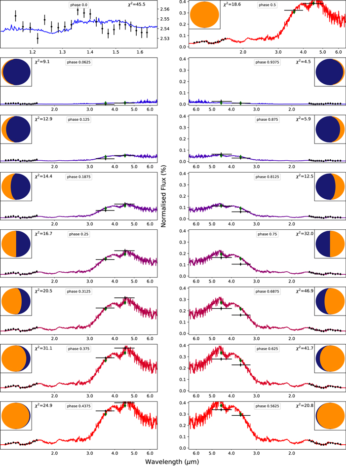
Figure 20. Best-fit spectra and geometry of our WASP-43 b phase curve retrieval with the two-faces free chemistry model. The temperature is described by the N-point free profile and the chemistry is coupled between the day and night sides. The diamonds represent the averaged Spitzer bandpasses. The right panels have an inverted wavelength axis.
Download figure:
Standard image High-resolution image
Figure 21. Temperature structure in the two-faces free scenarios for the day side (top) and night side (bottom). Blue: two-faces free chemistry with a free T–p profile and coupled chemistry; orange: two-faces free chemistry with the Guillot (2010) profile and coupled chemistry; green: two-faces free chemistry with a free T–p profile and decoupled chemistry.
Download figure:
Standard image High-resolution image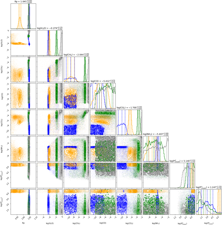
Figure 22. Posteriors distribution of the day-side chemistry and the properties of the clouds for the two-faces free runs. Blue: two-faces free chemistry with a free T–p profile and coupled chemistry; orange: two-faces free chemistry with the Guillot (2010) profile and coupled chemistry; green: two-faces free chemistry with a free T–p profile and decoupled chemistry (main solution). The latter retrieval also converged to a high mean molecular weight solution (shown in gray), which is discarded from our assumption of the primary atmosphere for this planet.
Download figure:
Standard image High-resolution image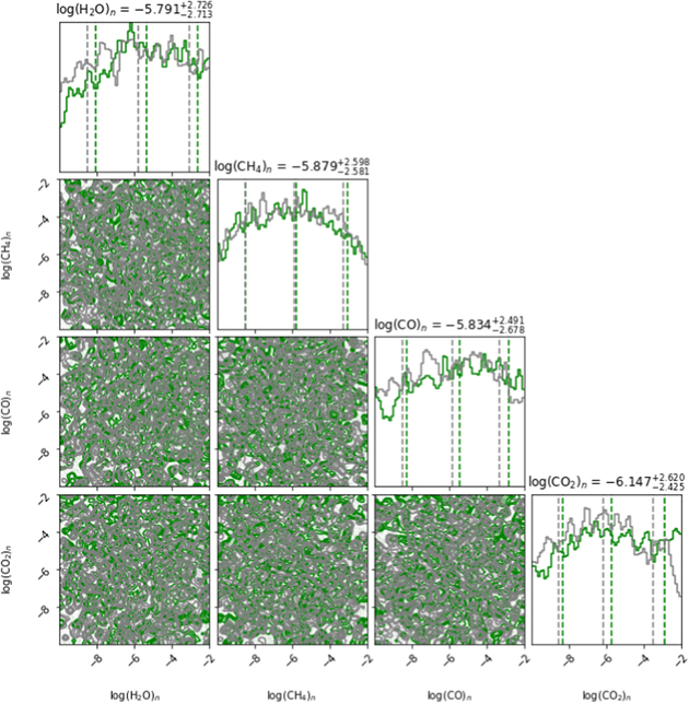
Figure 23. Posterior distribution two-faces free chemistry with a free T–p profile and decoupled chemistry. Green: main solution; gray: high mean molecular weight solution. The night-side chemistry posteriors do not lead to the detection of molecules for this run.
Download figure:
Standard image High-resolution imageAppendix H: Complementary Plots of the Two-faces Equilibrium Chemistry Retrieval
We show the best-fit spectra of our 2-faces equilibrium retrieval in Figure 24, the molecular abundances in Figure 25, the thermal structure in Figure 26m and the posterior distributions in Figure 27.

Figure 24. Best-fit spectra and geometry of our WASP-43 b phase curve retrieval with the two-faces equilibrium chemistry model. The diamonds represent the averaged Spitzer bandpasses. The right panels have an inverted wavelength axis.
Download figure:
Standard image High-resolution image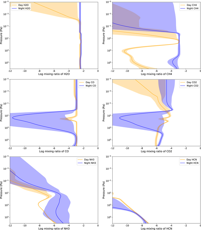
Figure 25. Molecular abundances in the different regions of the two-faces run, according to the chemical equilibrium scheme. Orange: day side; blue: night side.
Download figure:
Standard image High-resolution image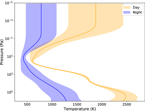
Figure 26. Temperature structure in the two-faces equilibrium scenario.
Download figure:
Standard image High-resolution image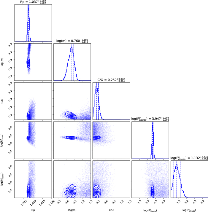
Figure 27. Posteriors distribution of the chemistry and the properties of the clouds for the two-faces equilibrium chemistry run.
Download figure:
Standard image High-resolution imageAppendix I: Complementary Plots the Full Model Retrieval (HST+Spitzer Against HST Only)
We show the best-fit spectra of our full retrieval in Figures 28 and 29, the retrieved thermal structure in Figure 30, and the posterior distributions in Figure 31.

Figure 28. Best-fit spectra and geometry of our WASP-43 b phase curve full retrieval. The colored spectrum is the same as Figure 2, zoomed around the HST wavelengths. The gray one corresponds to the HST-only retrieval. At the top, we show the transit (left) and the eclipse (right). The χ2 was calculated for the data between 1.1 and 1.7 μm only.
Download figure:
Standard image High-resolution image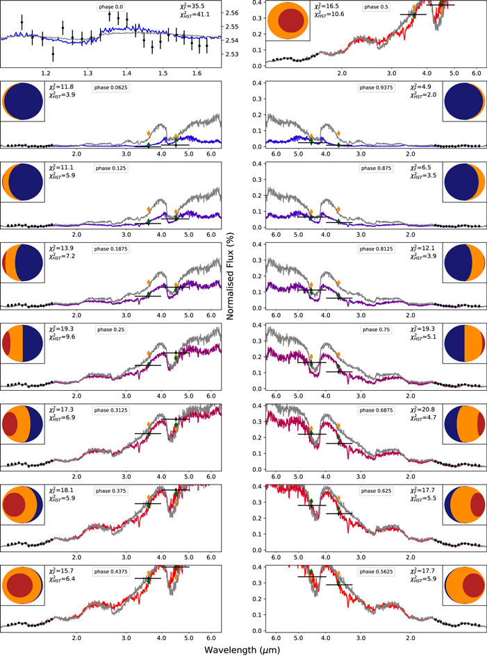
Figure 29. Best-fit spectra and geometry of our WASP-43 b phase curve retrieval. The colored spectrum is the same as in Figure 2. The gray one corresponds to the HST-only retrieval and shows the impact of adding the Spitzer data. At the top, we show the transit (left) and the eclipse (right). The diamonds represent the averaged Spitzer bandpasses (Orange: HST only; green: HST+Spitzer). The right panels have an inverted wavelength axis. The indicated  was computed from 1.1 and 1.7 μm only.
Download figure:
Standard image High-resolution image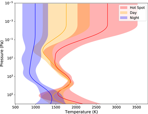
Figure 30. Temperature structure in the case of the HST-only retrieval. The 1σ error on the temperature profiles is much larger than in the HST+Spitzer case but the overall shape of those profiles is qualitatively consistent (see Figure 3).
Download figure:
Standard image High-resolution image
Figure 31. Posterior distribution of the chemistry and the properties of the clouds for the full run on the HST-only data. The retrieved metallicity reaches high values.
Download figure:
Standard image High-resolution imageAppendix J: Contribution Functions for the Full Scenario
Figure 32 shows the contribution functions of each region for the full scenarios. The contribution function is defined as  /dP, where
  is the transmittance.

Figure 32. Contribution functions of the hot spot (top), the day side (middle), and the night side (bottom) for the full run.
Download figure:
Standard image High-resolution imageAppendix K: Posterior Distributions of the Full Model for Different Hot-spot Sizes
Figures 33 and 34 show the posterior distributions of the full model using different hot-spot sizes.

Figure 33. Posteriors distribution of the chemistry and the properties of the clouds for the run with α = 30° (green), α = 40° (blue), and α = 50° (red).
Download figure:
Standard image High-resolution image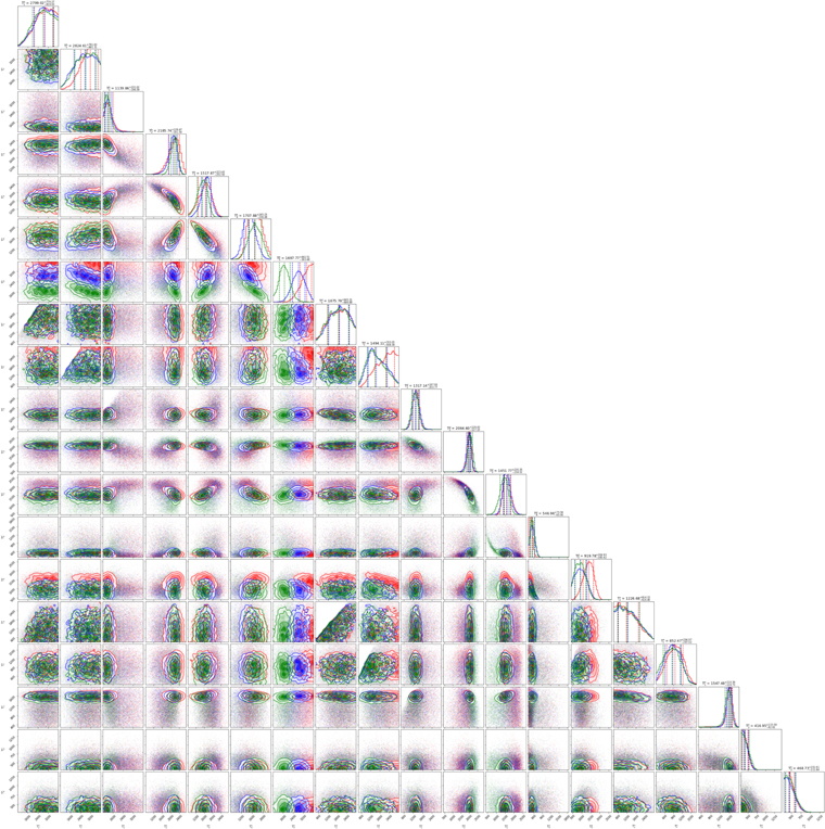
Figure 34. Posteriors distribution of the temperature points for the run with α = 30° (red), α = 40° (blue), and α = 50° (green). Because the T–p profile is smoothed, the actual profile does not intersect the retrieved pressure–temperature points.
Download figure:
Standard image High-resolution imageAppendix L: Results of the Full Model with Clouds Allowed on the Hot-spot
Figures 35, 36, and 37 respectively show the best-fit spectra, thermal structure, and posteriors for the full run where clouds are allowed on the day side.
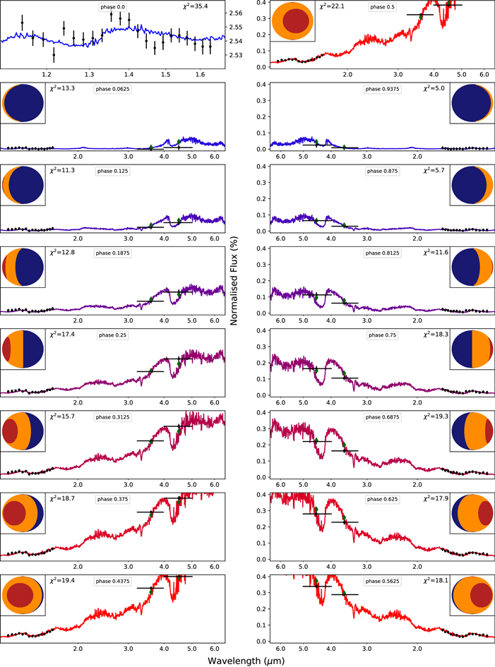
Figure 35. Best-fit spectra and geometry of our WASP-43 b phase curve retrieval with clouds allowed on the hot spot. At the top, we show the transit (left) and the eclipse (right). The diamonds represent the averaged Spitzer bandpasses. The right panels have an inverted wavelength axis.
Download figure:
Standard image High-resolution image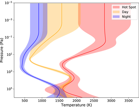
Figure 36. Temperature structure in the case of the HST+Spitzer retrieval with clouds allowed on the hot spot. Compared with the clear hot-spot model (see Figure 3), the uncertainties on the hot-spot temperature in the lower atmosphere are much larger.
Download figure:
Standard image High-resolution image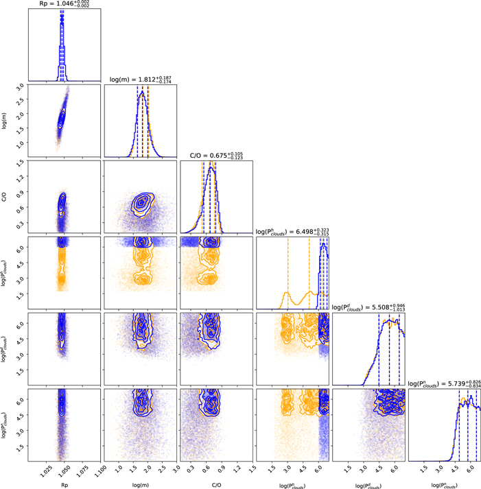
Figure 37. Posteriors for the chemistry and the cloud parameters in our runs with a fixed hot-spot size at 40°. In blue: clear hot spot (minimum cloud pressure forced at 106 Pa). In orange: cloud allowed on the hot spot.
Download figure:
Standard image High-resolution imageAppendix M: Results of the Full Model with 2500 Live Points
Figure 38 presents the posterior distributions for the full run with 2500 live points.

Figure 38. Posteriors for the chemistry and the cloud parameters in our full scenario with 2500 live points (Pink), compared with the standard run (Blue). While not shown, the temperature structure was also unchanged.
Download figure:
Standard image High-resolution image