


Abstract
The Chromospheric Lyman-Alpha Spectro-Polarimeter is a sounding rocket experiment that has provided the first successful measurement of the linear polarization produced by scattering processes in the hydrogen Lyα line (121.57 nm) radiation of the solar disk. In this paper, we report that the Si iii line at 120.65 nm also shows scattering polarization and we compare the scattering polarization signals observed in the Lyα and Si iii lines in order to search for observational signatures of the Hanle effect. We focus on four selected bright structures and investigate how the U/I spatial variations vary between the Lyα wing, the Lyα core, and the Si iii line as a function of the total unsigned photospheric magnetic flux estimated from Solar Dynamics Observatory/Helioseismic and Magnetic Imager observations. In an internetwork region, the Lyα core shows an antisymmetric spatial variation across the selected bright structure, but it does not show it in other more magnetized regions. In the Si iii line, the spatial variation of U/I deviates from the above-mentioned antisymmetric shape as the total unsigned photospheric magnetic flux increases. A plausible explanation of this difference is the operation of the Hanle effect. We argue that diagnostic techniques based on the scattering polarization observed simultaneously in two spectral lines with very different sensitivities to the Hanle effect, like Lyα and Si iii, are of great potential interest for exploring the magnetism of the upper solar chromosphere and transition region.
Export citation and abstract BibTeX RIS
1. Introduction
Spectropolarimetry is a unique observational technique for determining physical properties of astrophysical plasmas (e.g., magnetic fields). One physical mechanism for producing polarization in spectral lines is the Zeeman effect, which has been widely used. Recently, diagnostic techniques based on the Zeeman effect have been used to interpret high-spatial resolution observations under seeing-free conditions, such as those obtained with the spectropolarimeter (Ichimoto et al. 2008; Lites et al. 2013) of the Solar Optical Telescope (Shimizu et al. 2008; Suematsu et al. 2008; Tsuneta et al. 2008) on board the Hinode satellite (Kosugi et al. 2007) and IMaX (Martínez-Pillet et al. 2011) on board the Sunrise balloon telescope (Solanki et al. 2010). These observations have significantly advanced our empirical understanding of photospheric magnetic fields.
One of the key goals of solar physics is to understand how the hot plasma of the million-degree solar corona is produced and maintained (the so-called "coronal heating problem"). The chromosphere and the transition region, which are the interface layers between the photosphere and the corona, play a critical role in the energy balance of the outer solar atmosphere. Recent space-borne and ground-based observations revealed that this interface region is full of highly dynamic activities such as magneto-acoustic and Alfvén waves and jets, which could contribute to the heating of the upper chromosphere, transition region, and corona (e.g., Katsukawa et al. 2007; Okamoto et al. 2007; Shibata et al. 2007). However, lack of information on the magnetic field in this region limits the ability to quantify these phenomena. In the photosphere, the ratio of gas to magnetic pressure (β) is larger than unity; however, in the chromosphere and in the layers above, the magnetic forces dominate (i.e., β < 1). Hence, the magnetic structure of these upper layers is expected to be radically different from that of the photosphere, which in most cases can be measured using the Zeeman effect. Only by obtaining quantitative information on the strength and direction of the magnetic field in the low β regions of the solar atmosphere (chromosphere, transition region, and corona) will it be possible to decipher the magnetic coupling between the upper atmosphere and the underlying photosphere and to determine the relationship between the magnetic field and the dynamical activity of the upper atmospheric plasma.
The polarization of spectral lines originating in the solar chromosphere and above is sensitive to the presence of magnetic fields. However, because such spectral lines are broad and the magnetic fields there are expected to be weak, the polarization signals induced by the Zeeman effect are too small to be detected outside sunspots. As an alternative method, the Hanle effect (i.e., the magnetic-field-induced modification of the linear polarization caused by the scattering of anisotropic radiation; e.g., Casini & Landi Degl'Innocenti 2008) has been proposed for probing the magnetic field in the low β atmospheric regions because it is generally much more sensitive to weaker magnetic fields than the Zeeman effect. Recent developments in the theory and numerical modeling of polarization in spectral lines have suggested that the solar disk radiation of some ultraviolet (UV) lines that originate in the upper chromosphere and transition region should show measurable polarization signals caused by scattering processes and that, via the Hanle effect, the line-core polarization signals are sensitive to the presence of magnetic fields in such outer atmospheric regions (Trujillo Bueno et al. 2011, 2012; Belluzzi & Trujillo Bueno 2012). The hydrogen Lyα line at 121.57 nm is of particular interest because its core, which originates at the base of the transition region, is sensitive to the presence of magnetic fields with strength between approximately 10 and 100 G. The paper by Trujillo Bueno et al. (2011) motivated the development of the sounding rocket experiment Chromospheric Lyman-Alpha Spectro-Polarimeter (CLASP; see Kano et al. 2012; Kobayashi et al. 2012; Kubo et al. 2014). This rocket experiment was developed to measure the scattering polarization of the Lyα line and probe the magnetic field in the upper chromosphere and transition region via the Hanle effect. The first attempt to detect scattering polarization in UV lines, including Lyα, was conducted by Stenflo et al. (1980) using a slit-less instrument on board the Soviet satellite Intercosmos 16, but the mission was unsuccessful, presumably due to in-flight molecular contamination.
The CLASP instrument was launched on 2015 September 3 from White Sands Missile Range, and it successfully carried out observations during the 320 s of its suborbital flight. The CLASP observations, for the first time, demonstrated that there is indeed scattering polarization in the hydrogen Lyα line of the quiet solar disk radiation and that the measured Q/I and U/I core and wing signals have conspicuous spatial variations with scales of 10''–20'' (Kano et al. 2017). The Lyα wings, which are insensitive to the Hanle effect, showed scattering polarization perpendicular to the solar limb with a clear center-to-limb variation (CLV) and amplitudes as large as 6% near the limb, in agreement with the theoretical predictions (Belluzzi et al. 2012). On the other hand, the line core, where the Hanle effect operates, showed Q/I and U/I signals of the order of 0.1%, but without a clear CLV in Q/I, in contrast with the theoretical line-core polarization signals calculated using state-of-the-art 1D and 3D models of the solar atmosphere (Trujillo Bueno et al. 2011; Belluzzi et al. 2012; Štěpán et al. 2015). This discrepancy suggests that the geometrical complexity of the transition region, which is not realistic in such models, plays an important role on the Lyα scattering polarization (J. Štěpán et al. 2017, in preparation; J. Trujillo Bueno et al. 2017, in preparation).
It is necessary to disentangle the polarization induced by geometrical complexity and that induced by the magnetic field (i.e., the Hanle effect). One potential method is to observe simultaneously at least two spectral lines with different sensitivities to the Hanle effect, and ideally originating in the same region of the upper solar atmosphere (i.e., the so-called "differential Hanle effect"; e.g., Stenflo et al. 1998; Trujillo Bueno et al. 2012). To put it simply, the geometrical complexity would induce near-identical spatial variations of the polarization signals in the two lines, while the magnetic field would induce different modifications of the scattering polarization. Hence, a comparison of the observed polarization in the two lines would be a diagnostic of the magnetic field if the only difference between the two lines is their sensitivity to the magnetic field.
In this paper, we report the first detection of the scattering polarization in the Si iii line at 120.65 nm, along with observational insight on the causal relationship between the intensity and scattering polarization signals observed by CLASP. Finally, by comparing the U/I signals in the Si iii and Lyα lines, which have very different sensitivities to the Hanle effect, we show observational evidence in favor of the operation of the Hanle effect in these UV spectral lines.
2. Observations and Data Reduction
2.1. CLASP Observations
On 2015 September 3, CLASP observed a quiet region at the southwest limb during 280 s under stable pointing conditions in a sit-and-stare mode. The slit was roughly perpendicular to the solar limb with one edge covering an off-limb region of ∼20'' (see Figure 1(a)). The slit length is 400'' and its width is 1 45.
45.
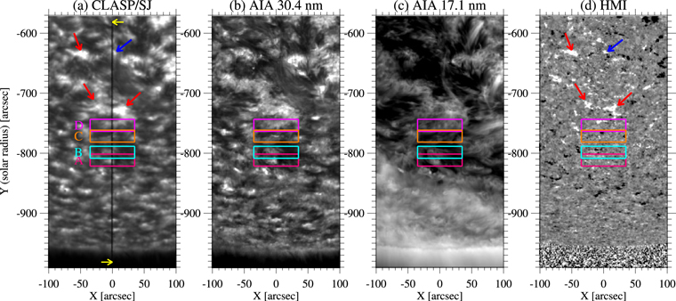
Figure 1. (a) CLASP/SJ image temporally averaged over 280 s. The dark vertical line indicates the CLASP slit, which is parallel to the Y axis. The yellow arrows indicate the slit edges. (b) Temporally averaged SDO/AIA 30.4 nm image. (c) Temporally averaged SDO/AIA 17.1 nm image. (d) Temporally averaged SDO/HMI longitudinal magnetogram ranging at ±30 Mx cm−2. These SDO images are spatially aligned to the CLASP/SJ image. The vertical axes indicate the radius from the Sun center, and a negative value means that the target region is located in the southern hemisphere. The horizontal axes indicate the distance from the slit. The red arrows show examples of bright structures surrounding a small filament (Section 2.3). The blue arrow shows a bright structure that the slit crosses and is located between filamentary structures. The regions A, B, C, and D indicated by colored boxes are the regions investigated in this work.
Download figure:
Standard image High-resolution imageCLASP has two optically symmetric channels, which provide two simultaneous measurements of orthogonal polarization states with two cameras (Narukage et al. 2015, 2017). The two cameras recorded the modulated intensity every 0.3 s in synchronization with the waveplate rotation. In addition to the hydrogen Lyα line at 121.57 nm (which was recorded by the two channels), one channel covered the Si iii line at 120.65 nm. After dark current subtraction, gain correction, and tilt correction of the spectrum, polarimetric demodulation was performed to derive the Stokes I, Q/I, and U/I of the Lyα and Si iii lines (see the
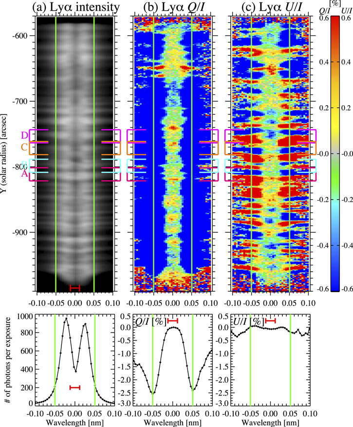
Figure 2. Top panels: Lyα spectra obtained by CLASP. The horizontal and vertical axes show the wavelength and solar radius, respectively. (a): intensity in logarithmic scale. (b) and (c): Q/I and U/I at ±0.6%. Regions A, B, C, and D in Figure 1 are indicated by the colored brackets. Lower panels: spatially and temporally averaged I (mean number of photons per exposure assuming that one electron corresponds to one photon), Q/I, and U/I in the Lyα line. In all panels, the red horizontal bar indicates the wavelength window chosen to calculate the line core I, Q/I, and U/I signals (within 0.012 nm from the nominal line center), while the green vertical lines indicate the wavelength positions chosen to calculate the wing I, Q/I, and U/I signals (at ±0.05 nm from the nominal line center). The green vertical lines indicate the wavelengths where the averaged Q/I shows maximum amplitude.
Download figure:
Standard image High-resolution imageThe plate scales are 11 per pixel along the slit and 0.0048 nm per pixel in wavelength. The spatial and spectral resolutions are estimated to be about 3'' and 0.01 nm, respectively (Giono et al. 2016b). Prior to the limb observation, CLASP conducted observations of the quiet Sun near the disk center for about 10 s in order to have data suitable for an in-flight polarization calibration (Giono et al. 2017). The Lyα spectra taken at the Sun center were averaged along the slit, and the pixel of the line center of the spatially averaged Lyα line is set to 121.567 nm. The spectra were found to move by 1 and 0.5 pixels along the dispersion direction in the two channels over the total observing duration of 320 s. However, we did not perform any correction for it since the influence of the gradual wavelength shift on the temporally averaged profiles is negligible.
2.2. Data from SDO
The Atmospheric Imaging Assembly (AIA, Lemen et al. 2012) on board the Solar Dynamics Observatory (SDO; Pesnell et al. 2012) takes full disk images of the solar atmosphere in multiple wavelengths. We choose the AIA 30.4 and 17.1 nm channels to study the transition region and lower corona, respectively. Their temporal cadence is 12 s and the plate scale is 06 per pixel. The AIA 30.4 nm channel provides an image that is very similar to the CLASP/slit-jaw optics system (SJ), as shown in Figures 1(a) and (b) (see Kubo et al. 2016 for more detail). Full disk measurements of photospheric line-of-sight (LOS) magnetic fields by the Helioseismic and Magnetic Imager (HMI, Scherrer et al. 2012) on board SDO are also used. Their temporal cadence is 45 s and the plate scale is 05 per pixel. Temporally averaged AIA and HMI images over the duration of the limb observations are shown in Figure 1. These images obtained by SDO are spatially aligned to the CLASP data by taking into account the pointing drift and jitter of the CLASP instrument.
2.3. Overview of Observing Region
The quiet region observed by CLASP was located near AR 12406 (see the CLASP/SJ image in Kubo et al. 2016). The slit center is located at (4681, −6258) in heliocentric coordinates, and the angle from the solar north–south direction is 37 43 in the counterclockwise direction. The CLASP/SJ and AIA images are rotated so that the CLASP slit is aligned to the vertical axes of Figure 1. The disk center part of the slit was covered by a small filamentary structure, as clearly seen in the AIA 30.4 and 17.1 nm images. This filament is surrounded by bright structures, as shown by the red and blue arrows in the CLASP/SJ images (Figure 1(a)). These bright structures are rooted in strong photospheric magnetic fields, which appear to be enhanced network fields (Figure 1(d)).
Along the slit, many bright structures are identified in the Lyα intensity spectra (Figure 2(a)), and the brightening penetrates the far wing (±0.1 nm from the line center). The bright structures become thicker toward the line center (i.e., higher in the atmosphere). This mustache-like structure (i.e., expansion of bright structure) suggests that the bright region dramatically expands with height in the chromosphere. In the bright regions near the limb (Y ≤ −880''), the central part of the mustache is distorted toward the limb. This is due to the fact that the core of the line forms higher than the wing.
3. Scattering Polarization in the Si iii Line
Figure 3 demonstrates that the core of the Si iii line shows significant linear polarization signals. The Q/I signals are predominantly negative (i.e., perpendicular to the solar limb) except for the region  . There is a bright structure around the center of this region (Y ∼ −635''), as shown in the intensity spectra (Figure 3(a)), and the positive Q/I signals are found in the dark regions besides the bright structure. This bright structure is indicated by a blue arrow in Figure 1, and it is sandwiched by a small dark filament. The large intensity gradient in these dark regions would induce the positive Q/I signals (a simple explanation is presented in the last paragraph of Section 4). The U/I signals consist of positive and negative patches along the slit, with no preferred sign.

Figure 3. Si iii line spectra observed by CLASP. (a): intensity in logarithmic scale. (b) and (c): Q/I at ±4% and U/I at ±1%. Pixels where the total number of photons collected during 280 s is smaller than 2 × 10⁴ are not shown in the Q/I and U/I spectra. The horizontal blue bars show the wavelength window (within 0.014 nm from the nominal line center) chosen to calculate the spatial variation of I, Q/I, and U/I for the Si iii line. The regions A, B, C, and D in Figure 1 are also indicated with colored brackets.
Download figure:
Standard image High-resolution imageFigure 4 shows the spatial variation of I, Q/I, and U/I in the Si iii line as well as in the Lyα core and wing. Since the Si iii line is weak compared with the Lyα line, we perform binning over 7 pixels along the wavelength direction indicated by a blue horizontal bar in the panels of Figure 3. The linear polarization in the Lyα core is of the order of 0.1%, and the I, Q/I, and U/I signals have also been averaged over the central 7 pixels indicated by the red horizontal bar in Figure 2. The Lyα wing I, Q/I, and U/I signals refer to the mean values of the pixels located at ±0.05 nm from the nominal Lyα center, and these pixels are indicated by green lines in Figure 2. In these pixels, the temporally and spatially averaged Q/I profile shows a maximum amplitude (see the lower middle panel of Figure 2). The uncertainties in Q/I and U/I are evaluated by  , where
  and
and  are the spurious polarizations caused by the photon noise and by the read-out noise of the CCD cameras. The equations to derive
  and
and  are the ones in Appendices A.1 and A.2 of Ishikawa et al. (2014b). We employ an averaged read-out noise of six electrons (Champey et al. 2014, 2015), which correspond to six photons. The averaged uncertainty is 0.066% at the Lyα core, 0.18% at the Lyα wing, and 0.50% at the Si iii line. In the Si iii line,
  and
and  are comparable, while
  is dominant both in the Lyα core and in the Lyα wing.
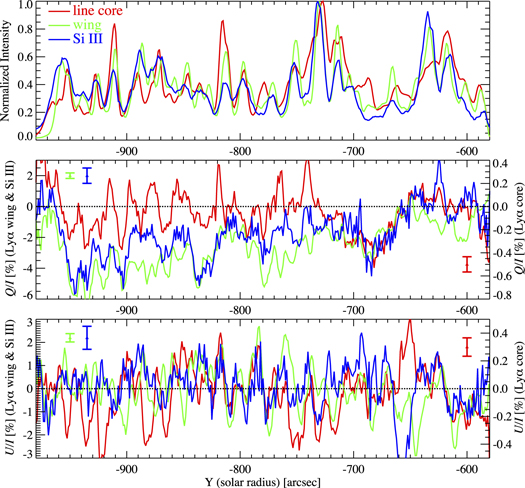
Figure 4. Spatial variation of I (normalized to the maximum intensity), Q/I, and U/I at the Lyα core (red), the Lyα wing (green), and the Si iii line (blue), calculated by averaging over the wavelength window specified in Figures 2 and 3. In the middle and bottom panels, the averaged uncertainties (±σ) of Q/I and U/I are shown using a red bar for the Lyα core (±0.066%), a green bar for the Lyα wing (±0.1%), and a blue bar for the Si iii line (±0.5%). In the middle and bottom panels, the vertical axes on the left show the Q/I and U/I signals in the the Lyα wing and the Si iii line, while the axes on the right show the ones in the Lyα core.
Download figure:
Standard image High-resolution imageThe Si iii line intensity observed by CLASP does not show a clear limb brightening or limb darkening. Its spatial variation along the slit is similar to that of the Lyα core and wing, which suggests that the Si iii line also originates in the upper chromosphere and the transition region. A recent theoretical investigation indicates that, at least for close to the limb lines of sight, the Lyα core and the Si iii line share the same region of formation (del Pino Alemán et al. 2017).
The I, Q/I, and U/I signals of the Si iii line show conspicuous spatial variations, and the typical spatial scale of the peak-to-peak variations is 10''–20''. The Q/I signals are dominated by negative values (i.e., linear polarization perpendicular to the solar limb), and they show a clear center-to-limb (CLV) variation, from −6% at Y ∼ −950'' to ∼0% at Y ∼ −600'', while the U/I signals fluctuate around zero (±2%). The dominance of negative Q/I signals with their clear CLV is also seen in the Lyα wing. The conspicuous spatial variation observed in I, Q/I, and U/I, with spatial scales of 10''–20'', is a common characteristic among the Lyα core, the Lyα wing, and the Si iii line.
When the reference direction for Stokes Q positive is chosen parallel to the nearest limb, the Q/I line-center signal produced by scattering process in a plane-parallel atmosphere without magnetic fields is approximately given by (e.g., Trujillo Bueno et al. 2011)


where  is a coefficient whose value depends on the angular momentum (j) of the lower (l) and upper levels (u) of the line under consideration and
  , with θ the heliocentric angle (Figure 5). While
  is the frequency-integrated mean intensity weighted by the absorption profile,
  quantifies whether the illumination of the atomic system is preferentially vertical or horizontal and it represents the axial symmetrical component of the anisotropic radiation field. In Equation (1), the degree of anisotropy,
  , which depends on the thermal and dynamic structure of the solar atmosphere, has to be evaluated where the line-center optical depth is unity along the LOS. Equation (1) indicates that Q/I = 0 at the disk center (μ = 1) and that the Q/I amplitude tends to be larger toward the limb (μ ∼ 0). Hence, the presence of CLV in Q/I is a defining characteristic of scattering polarization, whose amplitude is proportional to the anisotropy of the incident radiation field in the line-formation region.
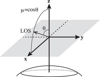
Figure 5. Geometry of the scattering event. The z-axis is normal to the solar surface, and the x–y plane is parallel to the solar surface. The line of sight (LOS) lies in the x–z plane. We choose the y-axis as the positive reference direction for Stokes Q, which is parallel to the nearest solar limb.
Download figure:
Standard image High-resolution imageThe Si iii line at 120.65 nm results from the transition between the ground level 3s2 1S0 and the  excited level (Table 1). The upper level has three magnetic sublevels with
  (m being the magnetic quantum number), which can harbor population imbalances and quantum coherence induced by the absorption and scattering of anisotropic radiation. Clearly, the linear polarization observed by CLASP in the Si iii line is scattering line polarization.
Table 1. List of Spectral Lines Studied in This Paper
| Wavelength (nm) | Line | Transition | Landé factor of upper level | Aul (s−1) |
|---|---|---|---|---|
| 121.57 | H i |
 − − 
|
4/3 |

|
| 120.65 | Si iii | 3s2 1S0 − 
|
1 |

|
Note. For each entry, we give the wavelength, the line identification, the line transition, the Landé factor of the upper level, and the Einstein Aul coefficient in s−1. The Landé factor is calculated using the L–S coupling scheme, while the other parameters are from the NIST database. For the hydrogen Lyα line, we only give the transition that contributes to its scattering polarization.
Download table as: ASCIITypeset image
For spectral lines like Lyα line and Si iii, only the upper level can be polarized, and the critical field strength for the onset of the Hanle effect, BH (in Gauss), is given by  , where gu is the level's Landé factor and Aul is the Einstein spontaneous emission coefficient in s−1. Using the parameters listed in Table 1, we have
  G for the Si iii line and
  G for the hydrogen Lyα line. In the Lyα wing,
  , since it is insensitive to the Hanle effect. The Lyα line starts to approach the Hanle saturation regime (i.e., the Q/I and U/I signals are only sensitive to the magnetic-field direction) above ∼50 G (see Ishikawa et al. 2014a). The simultaneous measurements of the scattering polarization in the Lyα and in the Si iii line with different sensitivities to the Hanle effect, provide more information to constrain the magnetic field with a larger sensitivity range than that only with the Lyα line.
4. Scattering Polarization Signals Due to the Local Anisotropic Radiation Field
In 1D plane-parallel semi-empirical models of the solar atmosphere, without magnetic fields, and taking the reference direction for positive Stokes Q parallel to the nearest solar limb, the U/I signals are zero (Equation (2)). This is because in such atmospheric models the incident radiation field has axial symmetry around the local vertical. The non-zero U/I signals observed by CLASP in the Lyα wing (Figure 2(c)), where the Hanle effect does not operate, suggest that the wing scattering polarization is caused by the symmetry breaking produced by the horizontal atmospheric inhomogeneities of the solar chromospheric plasma (i.e., that there are significant non-axisymmetric radiation fields). This is also supported by the intensity variations observed by CLASP along the slit, with scales of 10''–20'' similar to the variations seen in Q/I and U/I.
Figure 6 provides a detailed comparison between I, Q/I, and U/I at the Lyα wing. Here we focus on the part of the slit where we have quiet-Sun regions (i.e., Y < −710''). The Y locations where the intensity shows a local maximum (i.e., the core of bright structures) are indicated by yellow vertical lines. We find that, except in the gray-shaded areas, the peak locations coincide with those where U/I changes sign. As discussed below, this correspondence between peak intensity locations and zero-crossing points of U/I can be easily interpreted using a simple scattering polarization model where the anisotropy of the local radiation field plays a dominant role.
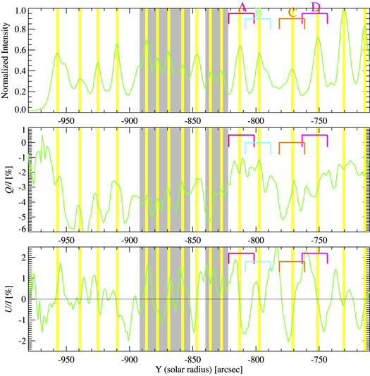
Figure 6. Spatial variation of I (normalized to the maximum intensity), Q/I, and U/I at the Lyα wing (i.e., the same green curves of Figure 4) by removing the region where there is a small filament (i.e., the region with Y > −710'' in Figure 1). Locations where the intensity presents a local maximum are indicated by yellow vertical lines. The gray-shaded areas show the ones where the intensity peak locations do not coincide with the zero-crossing points in U/I. Regions A, B, C, and D in Figure 1 are also indicated with colored brackets.
Download figure:
Standard image High-resolution imageIn a three-dimensional (3D) model of the solar atmosphere, the breaking of the axial symmetry of the radiation field illuminating the atomic system at each point within the medium also contributes to the scattering polarization (Manso Sainz & Trujillo Bueno 2011; Štěpán et al. 2015). As a result, Equations (1) and (2) do not hold, since without a magnetic field the mere presence of horizontal inhomogeneities can create U/I signals and modify the Q/I signals (e.g., at the solar disk center Q/I and U/I are not zero, in general). In particular, for the LOS indicated in Figure 5, U/I scattering polarization signals are produced by the presence of horizontal inhomogeneities, unless they are symmetric with respect to the x–z plane, resulting in non-zero U/I values. Here, we consider an isolated bright structure of circular shape observed at the solar disk center (see Figure 7). At the very center of a bright structure, the intensity gradient in the horizontal direction is zero. In other words, the symmetry axis of the radiation field is aligned with the LOS, and Q = U = 0. However, outside the center of the bright structure, the symmetry axis of the radiation field does not coincide with the μ = 1 LOS and non-zero scattering polarization signals arise. The resulting linear polarization is tangential to circles around the center of the bright structure and the Q and U signs are indicated in the lower panels of Figure 7. A similar illustrative example can be found in the bottom left panel of Figure 1 of Štepán & Trujillo Bueno (2012), which shows the disk center scattering polarization in the Lyα line core produced by relatively bright and dark structures of circular shape computed by means of a three-dimensional (3D), non-LTE multilevel radiative transfer code. When the spectrograph's slit hits a bright structure, as indicated by the gray line of Figure 7, we have  and U = 0 (i.e., U/I changes sign) at x = 0. Hence, the above-mentioned spatial variation of the U/I signals observed by CLASP in the Lyα wing results from the horizontal inhomogeneity caused by local bright structures. However, we also find exceptions at the gray-shaded areas, where the peak intensity locations do not coincide with zero-crossing points in U/I. In these areas the distance between bright structures is relatively small (≤10''), while outside it the typical distance is ∼20'', as shown in the top panel of Figure 6. In addition, the intensity enhancement of the bright structures located inside the gray-shaded areas is not as large as that outside. We speculate that positive and negative U/I signals over a bright structure are merged with positive and negative U/I signals in the next bright structure when the distance is small and a zero-crossing is not clearly visible.
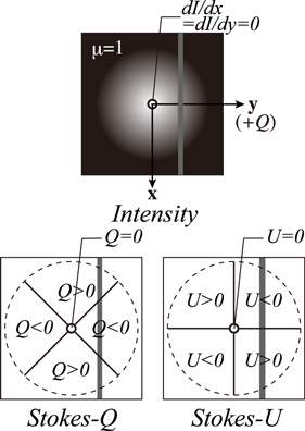
Figure 7. Schematic example of Q/I and U/I scattering signals produced at the disk center (lower panels) by a bright structure of circular shape (upper panel). The gray line shows an example of the spectrograph's slit locations crossing a bright structure.
Download figure:
Standard image High-resolution imageConcerning I and Q/I in the Lyα wing, we note that locations with local maximum in intensity roughly correspond to positions showing local maximum or minimum values in Q/I (see Figure 6). The interpretation of the spatial variation of the Q/I signals with respect to that of I is not so straightforward. As shown in Figure 7, in the idealized case of an isolated bright structure, Q has the largest negative value at x = 0 (where intensity is maximum), resulting in a local minimum. Thus, if the Q/I spatial variation is mainly due to the local symmetry breaking caused by bright structures, Q/I should show a local minimum at every U/I zero-crossing point (i.e., at every peak intensity location). Some cases in Figure 6 correspond to this situation (e.g., Y ∼ −812'' and Y ∼ −730''), but in others the peak intensity locations coincide with the locations where the Q/I has a local maximum (e.g., Y ∼ −800'' and Y ∼ −880''). In some cases, we find that the positions with a peak intensity lie between locations where Q/I has a local maximum or minimum value (e.g., Y ∼ −750'' and Y ∼ −925''). The axisymmetric component of the anisotropy  , which mainly induces the Q/I scattering polarization, could vary over the bright structure. This variation as well as the horizontal inhomogeneity due to the bright structure would contribute to a spatial variation of Q/I resulting in properties that cannot be explained only by the simple example of Figure 7.
The simple scattering polarization model (Figure 7) can also be applied to understand the positive Q/I in the Si iii line (Section 3). Let us assume that the slit crosses the center of the bright structure (i.e., it is located at  in Figure 7). In this case, at the edge of the bright structure (i.e., dark regions) along the slit, Q shows the largest positive signals. When the positive Q signals due to this local effect dominate the negative CLV signals, the net Q signals result in positive values even outside the disk center. As pointed out in Section 3, the positive Q/I signals in the Si iii line are found in the dark regions that surround the bright structure, and this observational signature is consistent with this simple model.
5. Indication of the Hanle Effect
5.1. Strategy
Clearly, the scattering polarization signals in the Lyα core, in the Lyα wings, and in the Si iii line are affected by the horizontal inhomogeneities of the solar atmosphere. In order to infer information on the magnetic field, we have to disentangle the Hanle effect from the breaking of the axial symmetry of the radiation field produced by the presence of the local horizontal inhomogeneities (Manso Sainz & Trujillo Bueno 2011; Štěpán et al. 2015). To this end, we focus on the spatial distributions of the U/I signals in bright regions where we understand their physical origin (Section 4). As discussed in Section 4, the sign of U/I changes around the center of each bright structure, namely, around the location where the intensity has a local maximum, and the relation between the intensity and U/I is interpreted as the consequence of the scattering polarization produced by the bright structure. Note that we focus only on the U/I spatial distribution, since the interpretation of the Q/I spatial distribution is not as straightforward as that of U/I (Section 4). Although there are several bright regions outside the gray-shaded areas, which also share this common feature, we investigate the four selected bright regions (Region A, B, C, and D) indicated by colored boxes in Figure 6. Figure 2(c) shows that near the limb (i.e., Y ≤ −900'') the alternate patterns of negative and positive U/I signals are not as clear as those in the regions indicated by colored boxes, and some of them do not show the symmetric U/I patterns in the Lyα wing. For example, at Y ∼ −920'', negative U/I signals dominate in the red wing, while negative signals are not clearly visible in the blue wing.
Another important reason to choose these four regions is that, in the Lyα core, the Si iii line, and the Lyα wing, they are seen as bright structures. Our simple explanation concerning why a bright structure causes a change in the sign of U/I is applicable to other spectral ranges. Hence, we assume that it applies to the Lyα core ( G), the Si iii line (
 G), and the Lyα wing (
 ) and this assumption allows us to identify the Hanle effect from the comparison of their polarized spectra, even though the line formation heights are not exactly identical.19
Similar U/I patterns are expected to be found in the Lyα core, in the Si iii line and in the Lyα wing, in the absence of magnetic fields. On the other hand, when a magnetic field is present, the Lyα core and/or the Si iii line will show the different behavior in the U/I signals from the Lyα wing, depending on the field strength.
) and this assumption allows us to identify the Hanle effect from the comparison of their polarized spectra, even though the line formation heights are not exactly identical.19
Similar U/I patterns are expected to be found in the Lyα core, in the Si iii line and in the Lyα wing, in the absence of magnetic fields. On the other hand, when a magnetic field is present, the Lyα core and/or the Si iii line will show the different behavior in the U/I signals from the Lyα wing, depending on the field strength.
If the Hanle effect leaves a clear signature in U/I, we expect to observe a magnetic structure in the photosphere. For this reason, we compare with the LOS photospheric magnetic flux measured by SDO/HMI. Although the four regions we have chosen are identified as bright regions in the Lyα and Si iii lines, their magnetic-field environments in the photosphere are different, given that they represent internetwork (Region A), network (Regions B and C), and enhanced network regions (Region D).
5.2. Comparison of Scattering Polarization
5.2.1. Region A
Figure 8(a) shows our first example; it is a bright structure around Y = −813'', indicated by a pink box in Figure 1. This bright structure is also identified in the intensity spectra of the Lyα and the Si iii lines (Figures 8(c) and (e)). The spatial variation of the intensities in the Lyα core, the Lyα wing, and the Si iii line around the bright region are shown in Figure 8(g), clearly indicating that these three spectral windows represent maximum values at Y = −813'' in the Lyα wing and the Si iii line and at Y = −815'' in the Lyα core.

Figure 8. Zoom-in of Region A, indicated by a pink box in previous figures. (a): AIA 30.4 nm image (Figure 1(b)). (b): longitudinal magnetogram taken by HMI (Figure 1(d)). Magnetic flux densities of  ,
,  , and
, and  are indicated by blue (positive) and red (negative) contours. The purple box indicates the region used to calculate the total unsigned magnetic flux. (c)–(f): Stokes spectra (I and U/I) of the Lyα line and the Si iii line (Figures 2 and 3). The Lyα U/I spectra and the Si iii U/I spectra range ±0.6% and ±1%, respectively. The red bar, the green lines, and the blue bar are the same as those in Figures 2 and 3, which indicate the pixels to calculate the Stokes signals at the Lyα core, the Lyα wing, and the Si iii line. (g) and (h): spatial distributions of the I and U/I signals at the Lyα core (red), the Lyα wing (green), and the Si iii line (blue), which are the same as in Figure 4.
Download figure:
Standard image High-resolution imageFigure 8(d) shows that a bright structure consists of a pair of negative and positive U/I patches in the Lyα wing. The same panel indicates that the U/I signals in the Lyα core also show the same distribution consisting of negative and positive patches. This behavior is also found in the Si iii line (see Figure 8(f)). These similarities in U/I distributions can be confirmed in Figure 8(h), where the U/I signals at three wavelength windows are plotted. The U/I signals in the Lyα core, in the Si iii line, and in the Lyα wing change sign around Y = −813''. Finally, the SDO/HMI magnetogram (Figure 8(b)) does not show any significant photospheric magnetic field.
We define now the following quantity,

with λ = core, wing, or Si iii. Then,  ,
,  , and
, and  represent the U/I signals in the Lyα core (red line in Figure 8(h)), in the Lyα wing (green line in Figure 8(h)), and in the Si iii line (blue line in Figure 8(h)), and k indicates pixels inside the gray area of Figure 8(h). Except for Region C where the outer edge is affected by another bright region, we choose pixels sandwiched by the locations where
  becomes maximum in the Lyα wing. With this definition,
  when the spatial variation is perfectly antisymmetric and
  approaches 1 when it deviates from the antisymmetric shape. Indeed, in this region,
  for all spectral windows;
  ,
,  , and
, and  .
.
In addition, we calculate the total unsigned magnetic flux in the photosphere as

where BLOS is the magnetic flux density observed by HMI, Δ s is the geometrical area corresponding to 1 pixel, and l represents the pixel whose absolute magnetic flux density is larger than 33 Mx cm−2 inside the purple box of Figure 8(b). The criteria of 33 Mx cm−2 is five times larger than the noise level, and the noise level is estimated by the standard deviation of the temporally averaged HMI magnetogram signals in the area where there is no conspicuous magnetic field (in a very quiet region). The total unsigned magnetic flux of Region A is  Mx. The criteria of 33 Mx cm−2 is stringent, resulting in smaller total magnetic flux, but we employ this criteria in order to take into account only magnetic concentrations that appear to be connected to the upper atmospheric layers.
5.2.2. Region B
The second example (Region B), indicated by a light blue box in Figure 1, consists of a few faint bright structures, as shown in Figure 9(a). By comparing the AIA 30.4 nm image (Figure 9(a)) with HMI magnetograms (Figure 9(b)), it seems that such bright structures are rooted to three magnetic concentrations with negative polarity enclosed by red contours. To calculate the total unsigned magnetic flux  , we consider the purple box region indicated in the figure, which includes such magnetic concentrations. The total magnetic flux is about 100 times larger than that of Region A, with
  Mx.
Mx.
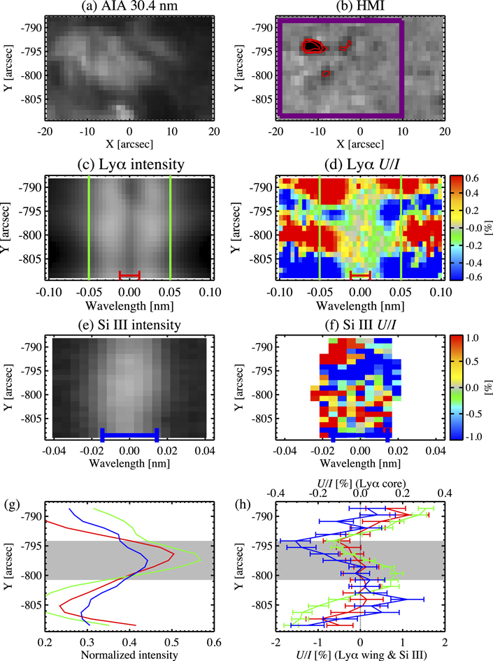
Figure 9. Zoom-in of Region B, indicated by a light blue box in Figures 2 and 3. For descriptions of the plots, see the caption of Figure 8.
Download figure:
Standard image High-resolution imageOne part of these bright structures is seen in the intensity spectra of the Lyα and the Si iii lines (Figures 9(c) and (e)), and all spectral regions show a clear peak around Y = −797'', as shown in Figure 9(g). This bright region shows negative U/I around Y = −795'' (at the disk center side) and positive U/I around Y = −800'' (at the limb side) in the Lyα wing (Figure 9(d)). However, the U/I signal at the Lyα core is almost zero. In the Si iii U/I spectra, the strong negative signals are seen around Y = −795'', but positive and negative signals are mixed around Y = −800'' (Figure 9(f)).
Figure 9(h) shows their spatial variations more clearly. In the Lyα wing,  changes sign around Y = −797'', with negative signals at the disk center side of the bright structure (
 ) and positive ones at the limb side (
 ). Similarly,
  shows negative signals at the disk center side (
 ) with a maximum amplitude of 1.5%. However, at the limb side (−802'' < Y − 799''), where positive
  signals are observed, the
  signals are fluctuating at ±0.2%. The behavior of the Lyα core is essentially the same as that of the Si iii line; the
  signals are negative at the disk center side with a maximum amplitude of 0.1% but are fluctuating around zero at the limb side. In summary, negative U/I signals are present, but positive U/I signals are seriously suppressed both in the Si iii and in the Lyα core. The different behavior of the Lyα core and the Si iii line from that of the Lyα wing are clearly indicated also by the
  quantity (Equation (3)), which is
  and
and  , while
  .
.
5.2.3. Region C
The third example is Region C, indicated by the orange box of Figure 1, while enlarged images of this region are shown in Figure 10. Here we focus on the bright structure located at Y ∼ −771'' (Figure 10(g)). As seen in Figure 10(d), the U/I signal at the Lyα wing changes sign (positive at the disk center side and negative at the limb side) over the bight structure (see also intensity spectra of Figure 10(c)). On the other hand, the Lyα core does not show such a change of the sign, since it is dominated by positive signals. The U/I signal of the Si iii line changes its sign, as shown in Figure 10(f). These behaviors of the U/I signals can also be seen in Figure 10(h). Both, the U/I signals of the Lyα wing and of the Si iii line change sign around Y = −770'', where their intensities are the largest, while the U/I signal of the Lyα core is dominated by positive values.
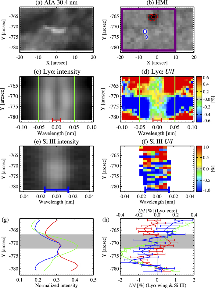
Figure 10. Zoom-in of of Region C, indicated by an orange box in Figures 2 and 3. For descriptions of the plots, see the caption of Figure 8.
Download figure:
Standard image High-resolution imageThe gray area to calculate  in Region C has been carefully chosen. Region D, which is next to Region C at the disk center side and is brighter than Region C, shows positive U/I at the limb side and negative U/I at the disk center side (see Figure 6). We deduce that the positive U/I signal of Region C at the disk center side is merged with the positive U/I signals of Region D and that it is impossible to identify the pixel where
  becomes maximum. Hence, we choose the location where the gradient of U/I becomes flat (Y = −767'') as the upper boundary of the gray area. Regarding the lower boundary, we investigate the spatial variation of I and U/I in the Lyα core. Around Y = −779'', only the Lyα core intensity shows a peak (Figure 10(g)). At the same location, U/I in the Lyα core crosses zero (Figure 10(h)). Assuming that the negative U/I signal in the Lyα core at −779'' < Y < −774'' is associated with the intensity peak at Y = −779'', we exclude this area to calculate
  .
.  for the Lyα wing and the Si iii line are close to zero (
 and
and  ) since they show the antisymmetric patterns, but
  .
.
In the photosphere, negative and positive magnetic concentrations are identified around [X, Y] = [−2'', −765''] and [X, Y] = [−7'', −773''], respectively. The prominent bright structure is elongated in the  direction as shown in the AIA 30.4 nm image of Figure 10(a), and it appears to be associated with the positive magnetic concentration. However, this bright structure is surrounded by a faint bright region, and we cannot deny that the targeting bright structure is not associated with the negative magnetic concentration. Therefore, to calculate total unsigned flux, we employ the purple box, which accommodates both negative and positive magnetic concentrations, resulting in
  Mx.
Mx.
5.2.4. Region D
The fourth example is a bright area that spreads throughout the small area of 40'' × 10'' seen in the AIA 30.4 nm image (Figure 11(a)). This bright region consists of elongated structures along the solar radial direction (i.e., the Y axis in the figures), and appears to be rooted in the positive magnetic concentrations at Y ∼ −748'' observed by the HMI magnetogram (Figure 11(b)). As discussed in Section 2.3, these magnetic concentrations correspond to the enhanced network field (see also Figure 1(d)), and the total unsigned magnetic flux is the largest among the four considered regions, with  Mx.
Mx.
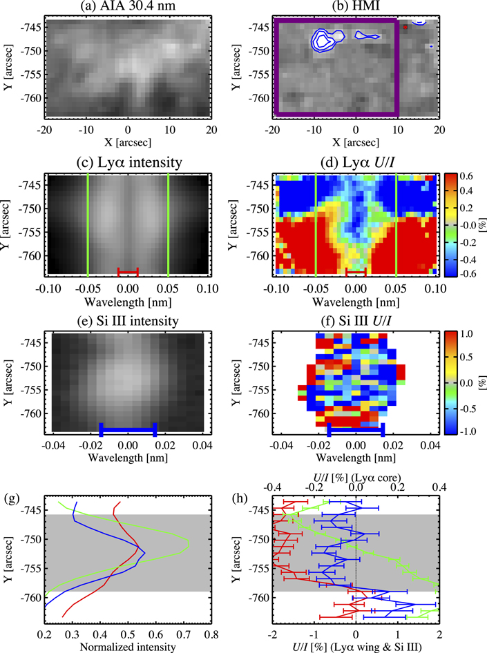
Figure 11. Zoom-in of Region D, indicated by the magenta box of Figures 2 and 3. For descriptions of the plots, see the caption of Figure 8.
Download figure:
Standard image High-resolution imageThe central part of this bright region can be seen in the intensity spectra of the Lyα and Si iii lines (Figures 11(c) and (e)); its maximum value is located at Y = −751'' in the Lyα core and wing and at Y = −752'' in the Si iii line (Figure 11(g)). Figure 11(d) clearly shows that the U/I signal in the Lyα wing changes sign over the bright structure, being negative at the disk center side and positive at the limb side. However, in the Lyα core and in the Si iii line, U/I is predominantly negative, as shown in Figures 11(d) and (f) (see also Figure 11(h)). In this example, the antisymmetric spatial distribution of the U/I signal in the Lyα core and in the Si iii line is not present, resulting in  and
and  , while
  .
.
5.3. Summary of Four Examples
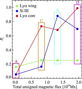
Figure 12 shows  versus
  for the A, B, C, and D selected regions. The quantity
  defined in Equation (3) quantifies how close the spatial distribution of the U/I signals is to the antisymmetric shape, while
  defined in Equation (4) is the total unsigned photospheric magnetic flux beneath each region. In these regions, the U/I signals in the Lyα wing clearly change sign over the bright structure, and their spatial distributions are antisymmetric. Thus, the
  quantity shows values close to zero in all regions (green circles in Figure 12).
Figure 12.
 vs.
vs.  in the four regions indicated in Figure 1. The region names (A, B, C, and D) are labeled at the periphery of each colored box. Red, green, and blue circles indicate Pcore (Lyα core), Pwing (Lyα wing), and
  (Si iii), respectively.
Download figure:
Standard image High-resolution image
In Region A, where  has its smallest value, the Lyα core and the Si iii line show antisymmetric distributions similar to those seen in the Lyα wing, and
  and
and  are also close to zero. No significant photospheric magnetic field is observed in Region A, which can be categorized as an internetwork region. Region C, which has the second lowest
  , harbors magnetic concentrations that correspond to the network fields. The U/I signal in the Si iii line maintains the antisymmetric shape (
 ), while the Lyα core does not (
 ). In Region B, which has the second highest photospheric magnetic flux, relatively strong network fields are observed. The antisymmetric shape of the U/I spatial distributions is partially lost in the Lyα core and in the Si iii line, resulting in
  and
and  . In Region D, which shows the highest
  and corresponds to an enhance network field region, the spatial distributions of U/I in the Lyα core and in the Si iii line do not show the antisymmetric shape, and they have
  and
and  .
.
The spatial variation of U/I in the Lyα core is similar to that in the Lyα wing only in the internetwork region (Region A), while the antisymmetric distributions are not seen in Regions B, C, and D, where network elements are present. The spatial variation of U/I in the Si iii line is similar to that in the Lyα wing in two regions with the smallest total unsigned photospheric magnetic fluxes. The deviation from the antisymmetric distribution is the larger the greater the unsigned photospheric magnetic flux.
6. Conclusions
6.1. Detection of Scattering Polarization in the Si iii 120.65 nm Line
Recently, Kano et al. (2017) reported the discovery of scattering polarization in the hydrogen Lyα line, obtained with CLASP. Here we have shown that CLASP has additionally detected scattering polarization in the Si iii line at 120.65 nm. We have compared it with the Lyα line-core and line-wing signals. The Si iii line shows significant linear polarization with a conspicuous spatial variation of 10''–20''. The Q/I signals observed in the Si iii line are predominantly negative (linear polarization perpendicular to the limb) and increasing toward the limb, where we find values of about −6%, while the U/I signals are fluctuating around zero with amplitudes of a few percent. These properties are similar to those observed in the Lyα wing. The polarizability of the Si iii line at 120.65 nm is the largest possible one (it is a line transition with  and
and  ; see Table 1) and it is clear that the measured linear polarization is due to scattering processes in the line forming region.
6.2. Scattering Polarization Caused By the Local Anisotropic Radiation Field
The Hanle effect does not operate in the Lyα wing, but there are sizable linear polarization signals caused by the scattering of anisotropic radiation. The presence of U/I signals in the Lyα wings suggests that the wing scattering polarization is affected by the local anisotropic radiation field induced by the horizontal inhomogeneities of the solar chromospheric plasma. We have found that in isolated bright regions, U/I in the Lyα wing changes sign around the peak intensity location where the intensity gradient is minimum, and the spatial variation of U/I over the bright structure is antisymmetric consisting of negative and positive U/I patches. This curious U/I behavior is compatible with the U/I signals produced by a bright structure. We have established the causal relationship between the U/I and I signals.
6.3. Indication of the Hanle Effect
We have compared the scattering polarization observed by CLASP in three characteristic wavelength windows: the Lyα core, the Lyα wing, and the Si iii line, which have different sensitivities to the Hanle effect. We have focused our attention on four bright regions labeled A, B, C, and D. The HMI magnetograms indicate that Region A is an internetwork region, Regions B and C are network regions (Region B has larger photospheric magnetic flux than Region C), and Region D is an enhanced network region with the largest photospheric magnetic flux.
The Lyα wing shows the above-mentioned U/I antisymmetric spatial distribution, which is caused by the presence of a bright structure in all selected regions, regardless of the total unsigned photospheric magnetic flux. Interestingly, only in the internetwork region (Region A) the U/I signal in the Lyα core behaves as in the Lyα wing (antisymmetric spatial distribution of U/I). In other regions, where larger photospheric magnetic fluxes are present, the spatial distributions of the U/I signals are different from that seen in the Lyα wing, and the antisymmetric shapes are not maintained. Such a different behavior of U/I from that in the Lyα wing is also found in the Si iii line, but only in the relatively strong network region (Region B) and in the enhanced network region (Region D).
The relation between the total unsigned photospheric magnetic flux and the U/I behavior, depending on the considered spectral window (Figure 12), can be naturally explained by the operation of the Hanle effect, which produces a rotation of the linear polarization plane. Considering the level's radiative time, i.e., Aul, the critical field strength for the onset of the Hanle effect in the Si iii line is  G, while
  G in the Lyα core and
  in its wings. In the internetwork region (Region A), the magnetic field in the upper chromosphere and the transition region is so weak that the Hanle effect does not produce a significant impact, neither in the Lyα core nor in the Si iii line. In the weaker network region (Region C), the field strength is expected to be too weak for the operation of the Hanle effect in the Si iii line, but sufficient to produce a measurable impact in the Lyα core. In Regions B and D, the magnetic field is strong enough to influence both the Si iii line and the Lyα core. In Region B, the antisymmetric shape is partially maintained in the Lyα core and in the Si iii line. This suggests that the magnetic field is not uniformly distributed over the bright structures and only the part where the spatial distribution of U/I deviates from the antisymmetric shape has a sufficiently strong magnetic field so as to induce the Hanle effect. Providing quantitative values would require confrontations with detailed radiative transfer modeling.
In this paper, we have presented observational evidence for the operation of the Hanle effect, by comparing the U/I signals observed by CLASP in two lines with different sensitivities to the Hanle effect: the Si iii 120.65 nm line and hydrogen Lyα. In general, the interpretation of the scattering polarization and the Hanle effect is a difficult task since the anisotropic radiation field and the Hanle effect are coupled. Here we have applied a new method based on comparing the U/I signals of the Lyα wing, the Lyα core, and the Si iii line in selected bright regions, where the symmetry breaking effect produced by the horizontal inhomogeneities of the solar chromosphere is assumed to be similar among these spectral windows. Our observational study emphasizes that ultraviolet spectropolarimetry is indeed a suitable diagnostic window that we should pursue further to probe the magnetism of the upper chromosphere and transition region of the Sun.
The Chromospheric Lyman-Alpha Spectropolarimeter (CLASP) team is an international partnership between NASA Marshall Space Flight Center, National Astronomical Observatory of Japan (NAOJ), Japan Aerospace Exploration Agency (JAXA), Instituto de Astrofísica de Canarias (IAC), and Institut d'Astrophysique Spatiale; additional partners include Astronomical Institute ASCR, Istituto Ricerche Solari Locarno, Lockheed Martin, and University of Oslo. The Japanese participation was funded by the basic research program of ISAS/JAXA, internal research funding of NAOJ, and JSPS KAKENHI (Grant Numbers 23340052, 24740134, 24340040, and 25220703). The US participation was funded by NASA Low Cost Access to Space (Award Number 12-SHP 12/2-0283). The Spanish participation was funded by the Ministry of Economy and Competitiveness through project AYA2010-18029 (Solar Magnetism and Astrophysical Spectropolarimetry). The French hardware participation was funded by Centre National d'Etudes Spatiales (CNES). J.Š. acknowledges the financial support by the Grant Agency of the Czech Republic through grant 16-16861S and project RVO:67985815. J.T.B. acknowledges the supercomputing grants provided by the Barcelona Supercomputing Center.
Appendix: Data Reduction
The half-waveplate optimized for the hydrogen Lyα line (Ishikawa et al. 2013) is located at the upstream of the slit. The waveplate continuously rotates at 4.8 s/rotation with a polarization modulation unit (PMU, Ishikawa et al. 2015), which generates a trigger signal regularly every 0.3 s. Each camera in the spectropolarimeter then takes 16 images with an exposure time of 0.3 s for every rotation synchronously with the waveplate rotation. Examples of observed signals in each camera can be found in Table 2 of Ishikawa et al. (2014b, note that the positive direction for Stokes Q in this table is parallel to the slit).
The first data reduction process includes the dark current subtraction, the gain correction, and the tilt correction of the image (i.e., rotate the image so that the dispersion and the slit are aligned to the pixel). After the alignment between the two channels, the demodulation is performed for each channel using all data, and that the positive Q-direction is defined to be perpendicular to the slit;


where  indicates the data at the jth exposure in ith channel, and t1 corresponds to the exposure over the PMU angle from 0° to 225. Finally, we derive fractional polarizations (Q/I and U/I). For the Lyα line,


where a = 2/π is a modulation coefficient resulting from the continuous rotation of the half-waveplate (i.e., phase retardation is equal to 180°) and Ki is the throughput value of each channel derived by summing all signals around the Lyα from the whole observing duration at the limb. For the Si iii line, by forming the single channel demodulation,


where  is the modulation coefficient for the Si iii line. The birefringence of MgF2, which is the material of the waveplate, is known to dramatically change in VUV (Johnson 1964; Chandrasekharan & Damany 1969). Using the wavelength variation of the birefringence (Chandrasekharan & Damany 1969; Laporte et al. 1983) the phase retardation at 120.65 nm is estimated to be 117°. Combining on-the-ground and in-flight polarization calibrations, the instrumental polarization was measured to be negligibly small compared to our requirement (Giono et al. 2016a; Giono et al. 2017). Hence we do not apply additional calibration to the demodulated data.
From the CLASP Slit-Jaw (SJ) image, the angle between the slit and the solar radius (Δα) turns out to be 16. This misalignment results in an azimuth error, i.e.,  crosstalk when we define the demodulated Stokes signals as those in the reference frame that the positive reference direction for Stokes Q is parallel to the solar limb. The crosstalk is ∼sin(2Δα)p, where p is the typical linear polarization degree. This crosstalk is comparable to or smaller than the noise level
  , as is the case with each of the quantities given in Table 2. Hence, we do not perform any additional calibration for the demodulated polarization signals, and the positive Q-direction is defined as the parallel to the solar limb.
Table 2. Typical Degree of Linear Polarization (p) and Noise Level (ε) in Each Wavelength Range
| Wavelength Range | p | |
|---|---|---|
| Lyα core | ≲0.5% | ∼0.07% |
| Lyα wing | ≲5% | ∼0.2% |
| Si iii | ≲5% | ∼0.5% |
Download table as: ASCIITypeset image
Footnotes
- 19
While the Lyα core originates at the base of the transition region, the nearby Lyα wings considered in this work originate a few hundreds of kilometers below (see the right panel of Figure 1 of Belluzzi et al. 2012). The core of the Si iii line originates close to the transition region (del Pino Alemán et al. 2017).