


Abstract
We present a census of variable stars in six M31 dwarf spheroidal satellites observed with the Hubble Space Telescope. We detect 870 RR Lyrae (RRL) stars in the fields of And I (296), II (251), III (111), XV (117), XVI (8), and XXVIII (87). We also detect a total of 15 Anomalous Cepheids, three eclipsing binaries, and seven field RRL stars compatible with being members of the M31 halo or the Giant Stellar Stream. We derive robust and homogeneous distances to the six galaxies using different methods based on the properties of the RRL stars. Working with the up-to-date set of Period-Wesenheit (I, B–I) relations published by Marconi et al., we obtain distance moduli of μ0 = [24.49, 24.16, 24.36, 24.42, 23.70, 24.43] mag (respectively), with systematic uncertainties of 0.08 mag and statistical uncertainties <0.11 mag. We have considered an enlarged sample of 16 M31 satellites with published variability studies, and compared their pulsational observables (e.g., periods and amplitudes) with those of 15 Milky Way satellites for which similar data are available. The properties of the (strictly old) RRL in both satellite systems do not show any significant difference. In particular, we found a strikingly similar correlation between the mean period distribution of the fundamental RRL pulsators (RRab) and the mean metallicities of the galaxies. This indicates that the old RRL progenitors were similar at the early stage in the two environments, suggesting very similar characteristics for the earliest stages of evolution of both satellite systems.
Export citation and abstract BibTeX RIS
1. Introduction
RR Lyrae variable stars (RRLs) are unambiguous stellar tracers of an old (>10 Gyr) stellar population. As such, they are a fossil record of the early stages of galaxy evolution. Their pulsational properties and their position in the color–magnitude diagram (CMD)—on the horizontal branch (HB), ∼3 mag above the old main-sequence turnoff—make RRLs easily identifiable objects even beyond the Local Group (LG; Da Costa et al. 2010). They are excellent distance indicators, and powerful tools to investigate the early evolution of the host stellar system, since their metallicity can be inferred from their pulsational properties (see e.g., Jeffery et al. 2011; Nemec et al. 2013; Martínez-Vázquez et al. 2016a, and references therein). Thus, RRL can provide valuable information on the nature of the building-blocks of large galaxies such as the Milky Way (MW) or M31 (see, e.g., Fiorentino et al. 2015; Monelli et al. 2017). Indeed, in the last few years, the study of the populations of RRL in galaxies has become increasingly relevant for research on galaxy formation and evolution in addition to the more classical field of stellar astrophysics.
Basically, RRL have been detected in all the dwarf galaxies where they have been searched for. At least one RRL has been found in all very low mass ( ;) dwarf spheroidal (dSph) galaxies (see, e.g., Baker & Willman 2015; Vivas et al. 2016 and references therein). In many brighter dSph galaxies (
 ), both satellites and isolated, the number of RRL is greater than ≈100. In this way, they are statistically sufficient to study in detail, for example, possible radial gradients in the old stellar populations of their host galaxies (e.g., Bernard et al. 2008; Martínez-Vázquez et al. 2015, 2016a). The great advance in observational studies of RRLs in nearby dwarf galaxies (see discussion in Section 5) has led to a much better understanding of their relative distributions in dwarf galaxies of different morphological type. The study of variable stars in satellites of the Andromeda galaxy (And, M31) is largely incomplete. This has been long due to two main reasons: (i) their (relatively) faint apparent magnitude (
 mag), and (ii) the stellar crowding. The first successful attempt to identify RRL stars in the M31 halo was achieved by Pritchet & van den Bergh (1987) using Canada–France–Hawaii telescope data. Saha & Hoessel (1990) and Saha et al. (1990) detected candidate RRL stars in the dwarf elliptical M31 satellites NGC 185 and NGC 147. Nevertheless, with the advent of the Hubble Space Telescope (HST), it was possible to reach well below the HB. This allowed the first determination of the properties of RRL stars in the M31 field and its satellites. Based on WFPC2 data, the discovery of RRL stars was reported in And I (Da Costa et al. 1996), And II (Da Costa et al. 2000), and And III (Da Costa et al. 2002). The population of variable stars detected in the three galaxies were later analyzed in detail by Pritzl et al. (2004, And II) and Pritzl et al. (2005, And I and And III). Additionally, And VI was studied by Pritzl et al. (2002) on the basis of data of comparable quality. Since then, the number of known satellites of M31 has increased dramatically, primarily due to the PAndAS survey (McConnachie et al. 2009). With a few exceptions (And XI, And XIII, Yang & Sarajedini 2012; And XIX; Cusano et al. 2013; And XXI; Cusano et al. 2015; And XXV; Cusano et al. 2016), most of them have not been investigated for stellar variability. Moreover, the knowledge of the properties of RRL stars in M31 itself and in the largest satellites (M32, M33) is limited to a few ACS fields and is far from being complete.
Under the ISLAndS16 project (based on very deep, multi-epoch HST ACS and WFC3 data), six M31 dSph satellite companion galaxies were observed: And I, And II, And III, And XV, And XVI, and And XXVIII. The main goal of this project is to determine whether the star formation histories (SFHs) of the M31 dSph satellites show notable differences from those of the MW. The project is described in more detail in the project presentation paper (Skillman et al. 2017), while the first results concerning the SFH of And II and And XVI were presented in Weisz et al. (2014) and Monelli et al. (2016).
In order to complement these previous studies, this paper focuses on the study of variable stars—mainly RRLs, but also Anomalous Cepheids (ACs)—present in the six ISLAndS galaxies. The data obtained within the framework of this project have allowed us to increase by a factor 2–3.4 the number of known variable stars and the quality of the light curves (LCs) in And I, And II, and And III compared to previous studies (Pritzl et al. 2004, 2005). On the other hand, this project provides the first discoveries of variable stars in And XV, And XVI, and And XXVIII, although an analysis of the RRL in AndXVI within the context of its SFH has been presented in Monelli et al. (2016); for homogeneity with the rest of the observed ISLAndS galaxies, in this work we reanalyzed the And XVI variable stars from scratch, obtaining slightly refined values.
This paper is structured as follows. In Section 2 we present a summary of the observations and data reduction. In Section 3 we describe the variable star detection and classification, while Section 4 focuses on the properties of RRL stars. The properties of the HB and of RRL stars of M31 satellites are compared to those of MW dwarfs in Section 5. RRL stars are used in Section 6 to derive new, homogeneous distances to the six galaxies. Furthermore, distance estimations based on the tip of the red giant branch (TRGB) are provided for the three most massive galaxies (And I, II, and III). Finally, ACs and eclipsing binary (EB) candidates are also presented in Sections 7.1 and 7.2, respectively. We note that in the online version of the paper we provide full details on all the variable stars discussed: time-series photometry, LCs, and mean photometric and pulsational properties.
2. Observations and Data Reduction
Table 1 presents a compilation of updated values for the position of the center (R.A. and decl., columns 2 and 3, respectively), absolute MV magnitude (column 4), reddening (E(B-V), column 5), and structural parameters—ellipticity ( , column 6), position angle (PA, column 7), half-light radius (rh, column 8), and tidal radius (rt, column 9)—for each of the six observed galaxies under the ISLAndS project (hereafter called ISLAndS galaxies).
Table 1. Positions and Structural Parameters for the ISLAndS Galaxies
| Galaxy | R.A. | Decl. | MV | E(B–V) |

|
PA | rh | rt | References |
|---|---|---|---|---|---|---|---|---|---|
| (name) | (hh mm ss) | (° ' '') | (mag) | (1-b/a) | (°) | (') | (') | ||
| And I | 00:45:39.7 | 38:02:15.0 | −11.2 ± 0.2 | 0.047 | 0.28 ± 0.03 | 30 ± 4 | 3.9 ± 0.1 | 10.4 ± 0.9 | 1, 2 |
| And II | 01:16:26.8 | 33:26:07.0 | −11.6 ± 0.2 | 0.063 | 0.16 ± 0.02 | 31 ± 5 | 5.3 ± 0.1 | 22.0 ± 1.0 | 1, 2 |
| And III | 00:35:30.9 | 36:29:56.0 | −9.5 ± 0.3 | 0.050 | 0.59 ± 0.04 | 140 ± 3 | 2.0 ± 0.2 | 7.2 ± 1.2 | 1, 2 |
| And XV | 01:14:18.3 | 38:07:11.0 |

|
0.041 | 0.24 ± 0.10 | 38 ± 15 | 1.3 ± 0.1 | ∼5.7 | 1, 3 |
| And XVI | 00:59:30.3 | 32:22:34.0 | −7.3 ± 0.3 | 0.066 | 0.29 ± 0.08 | 98 ± 9 | 1.0 ± 0.1 | ∼4.3 | 1, 3 |
| And XXVIII | 22:32:41.5 | 31:13:03.7 | −8.7 ± 0.4 | 0.080 | 0.43 ± 0.02 | 34 ± 1 | 1.20 ± 0.01 | ∼18.0 | 4, 5 |
References. (1) Martin et al. (2016), (2) McConnachie & Irwin (2006), (3) Ibata et al. (2007), (4) Slater et al. (2015), and (5) Tollerud et al. (2013).
Download table as: ASCIITypeset image
The data for these six ISLAndS galaxies have been obtained under proposals GO-13028 and GO-13739 for a total of 111 HST orbits. They consist of one ACS pointing on the central region and a WFC3 parallel field (at 6' from the ACS center) for each galaxy. For further details about the ACS and WFC3 field location, the reader is referred to Figure 4 of Skillman et al. (2017), where the strategy and the description of the ISLAndS project is explained in depth.
For both cameras, the  and
and  passbands were chosen. The observing strategy was designed in order to optimize the phase coverage of short-period variables (between 0.3 and 1.2 day), specifically, RRL and AC stars. In particular, the observations were spread over a few days (from two to five), and the visits were planned to avoid accumulation of data around the same time of day, in order to avoid aliasing problems around 0.5-day or 1-day periods. An overview of the observing runs is provided in Table 2, which specifies for each galaxy (column 1) the beginning and ending dates (column 2) and the number of orbits obtained (column 3). For an optimal sampling of the LCs, each orbit was split into one
  and one
  exposure, yielding the same number of epochs in each band for each galaxy. Detailed observing logs are presented in Appendix A (Table 9).
Table 2. Summary of HST Observations
| Galaxy | Obs. Dates | Orbits |
|---|---|---|
| And I | 2015 Sep 1–6 | 22 |
| And II | 2013 Oct 4–6 | 17 |
| And III | 2014 Nov 24–28 | 22 |
| And XV | 2014 Sep 17–20 | 17 |
| And XVI | 2013 Nov 20–22 | 13 |
| And XXVIII | 2015 Jan 20–25 | 20 |
Download table as: ASCIITypeset image
The photometry has been homogeneously performed with the DAOPHOT/ALLFRAME suite of routines, following the prescriptions described in Monelli et al. (2010), for both the ACS and parallel WFC3 fields. The photometric catalogs have been calibrated to the VEGAMAG photometric systems adopting the updated zero-points from the instrument web page.
3. Variable Star Identification
Candidate RRL stars and ACs were searched for in a rectangular region of the CMD with a width that covers the full color range of the HB, and with height between ∼1.5 mag fainter than the HB to the magnitude of the TRGB, i.e., enclosing the instability strip (IS) where RRL stars and ACs are located.17 We visually inspected the LCs of all the stars in this region, without any cut on a variability index. The number of candidates ranged from 201 in And XVI to 7414 in And I. The periodogram was calculated between 0.2 and 10 days, a range that encompasses all the possible periods of RRL stars and ACs. Pulsational parameters were derived for the confirmed variables sources. Using widget-based software, we first estimated the period of candidate variables through the Fourier analysis of the time series, following the prescription of Horne & Baliunas (1986). The analysis was refined by visual inspection of the LCs in both bands simultaneously in order to fine-tune the period. The intensity-averaged magnitudes and amplitudes of the mono-periodic LCs were obtained by fitting the LCs with a set of templates partly based on the set of Layden et al. (1999) following the procedure described in Bernard et al. (2009). We expect that the completeness of both the RRL star and AC samples are 100% within each pointing for the following reasons: (i) the search for candidates, described above, ensures that any star showing brightness variations has been visually inspected; (ii) according to the artificial star tests presented in Skillman et al. (2017), the photometric completeness at the magnitude of the HB (and above) is about 100%; and (iii) the amplitudes of the RRLs and ACs pulsations are significantly larger than the magnitude uncertainty in the region of the HB and above.
The classification of variable stars was based on their pulsational properties (period and amplitude), LCs, and positions on the CMD. Table 3 summarizes the total number of different types of variable stars detected. Most of them are RRL stars (870 in the dwarfs plus 7 field stars), while a few are ACs (15) and EBs (3). Each variable type is described in more detail in the subsequent sections.
Table 3. Variable Star Detections
| And I | And II | And III | And XV | And XVI | And XXVIII | Total | ||
|---|---|---|---|---|---|---|---|---|
| ACS | 261 | 217 | 108 | 117 | 8 | 87a | 798 | |
| RRL | WFC3 | 35 | 34 | 3 | 0 | 0 | 0 | 72 |
| total | 296 | 251 | 111 | 117 | 8 | 87 | 870 | |
| ACS | 0 | 4 | 4 | 4 | 0 | 3 | 15 | |
| AC | WFC3 | 0 | 0 | 0 | 0 | 0 | 0 | 0 |
| total | 0 | 4 | 4 | 4 | 0 | 3 | 15 | |
| ACS | 1 | 1 | 0 | 0 | 0 | 0 | 2 | |
| EB | WFC3 | 0 | 1 | 0 | 0 | 0 | 0 | 1 |
| total | 1 | 2 | 0 | 0 | 0 | 0 | 3 | |
| ACS | 5b | 0 | 1c | 0 | 1c | 0 | 7 | |
| Field | WFC3 | 0 | 0 | 0 | 0 | 0 | 0 | 0 |
| total | 5 | 0 | 0 | 0 | 1 | 0 | 7 | |
| TOTALACS | 267 | 222 | 113 | 121 | 9 | 90 | 822 | |
| TOTALWFC3 | 35 | 35 | 3 | 0 | 0 | 0 | 73 | |
| TOTAL | 302 | 257 | 116 | 121 | 9 | 90 | 895 | |
Notes.
aIncludes two stars with rather noisy light curves. Based on their position in the CMD, we assume they are RRL stars. bRRL (three RRab plus two RRc) stars compatible with being field stars of the GSS of M31. cRRab star compatible with a candidate field star from M31.Download table as: ASCIITypeset image
The individual  and
and  measurements (time series) for all the detected variables are available in Appendix B (Table 10). The typical photometric uncertainties on individual measurements are of the order of 0.07 mag and 0.06 mag in
  and
and  , respectively, for the most distant galaxy (And I), while for the nearest galaxy (And XVI), it is of the order of 0.04 mag in both passbands. The variable stars were named with a prefix that refers to the galaxy, followed by "V," indicating that the star is a variable (e.g., "And I–V"), and a number that increases with increasing right ascension. Interestingly, we note that no variable stars were detected in the parallel fields (WFC3) of And XV, And XVI, and And XXVIII, in agreement with the visual appearance of the CMD, which does not show any obvious evolutionary sequence (HB, RGB, or the more populous main-sequence turnoff). We also note that the RRL stars of And XVI have been presented in Monelli et al. (2016), but are included in this work as well for completeness. As some of our target galaxies have previously been investigated for variability (And I: Pritzl et al. 2005; And II: Pritzl et al. 2004; And III: Pritzl et al. 2005), a detailed comparison is presented in Appendix C.
The derived values of the pulsational properties (period, amplitudes, mean magnitudes) for the variable stars detected in the different galaxies are presented in Appendix D (Table 12). These tables include the star name, position (R.A., decl.), period, mean magnitude and amplitude in the  ,
,  , B, V, and I passbands, and the classification. We note that the HST magnitudes in the VEGAMAG system were transformed to the Johnson system using the calibration provided by Bernard et al. (2009). The main purpose of this conversion from
  and
and  magnitudes to Johnson BVI is not only to allow comparison with observations of variable stars in globular clusters (GCs) and other galaxies reported in the literature (see Section 5), but also to use the period–luminosity relations (for example, to obtain distances, as we do in Section 6) or the Bailey (period–amplitude) diagram (see Section 4), which are most commonly used in the V band.
We display in Figure 1 the CMDs of the ACS fields of the six galaxies, highlighting in them the different types of variable stars detected: RRL stars (blue star symbols for the dSph members and green open circles for field RRL stars), ACs (red circles), and EBs (magenta triangles). Table 3 displays the number of detected variables of each type in the ACS fields. The CMD of And I clearly shows the contamination of the M31 GSS (Ibata et al. 2001; Ferguson et al. 2002; McConnachie et al. 2003), as shown by the presence of a second, redder RGB and red clump visible in the CMD. In particular, we have found five RRL stars with properties compatible with membership in the GSS (see Section 4.2).
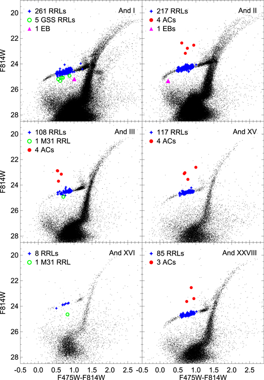
Figure 1. CMDs of the ACS fields for each ISLAndS galaxy. The And I CMD shows a significant contamination from the M31 GSS (Ibata et al. 2001; Ferguson et al. 2002; McConnachie et al. 2003). Variable stars are overplotted. Blue stars represent the RRL stars. Red circles are the ACs. Green open circles are RRL stars tentatively associated with the field of M31. Magenta triangles are the probable eclipsing binaries.
Download figure:
Standard image High-resolution imageRRLs were detected in all six galaxies with as few as 8 (in And XVI)18 and as a many as 296 (in And I). The striking difference in the number of RRL between And XVI and And XV, despite having a similar mass, can be explained as a consequence of their different SFHs: the mass fraction already in place at old ages (10 Gyr ago) was only about 50% in And XVI, while it was 90% in And XV (see Figure 7 in Skillman et al. 2017).
A few (3–4) ACs are present in And II, III, XV, and XXVIII, but none have been detected in And I or in And XVI. This is not surprising in the case of the latter because of its low mass.19 The lack of ACs is remarkable in the case of And I, however, as no other massive dSph presents such a dearth of ACs (see Section 7.1). Nevertheless, the high mean metallicity (Kalirai et al. 2010) may explain this occurrence.
Figure 2 presents the CMDs for the parallel WFC3 fields of And I, II, and III, where variable stars have been detected. The symbols are the same as in Figure 1. The presence of the GSS is also noticeable in the CMD of the parallel WFC3 field of And I. For the cases of And XV, XVI, and XXVIII, the parallel WFC3 fields do not show a significant component of the galaxy; in fact, no variable stars have been detected.
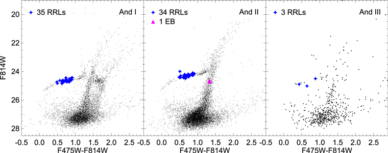
Figure 2. CMDs of the parallel WFC3 fields for the three ISLAndS galaxies that still have a relevant stellar population. Variable stars are overplotted. As in Figure 1, blue stars represent the RRL stars, and magenta triangles are the probable eclipsing binaries. In the case of the And I CMD, the contamination from the M31 GSS (Ibata et al. 2001; Ferguson et al. 2002; McConnachie et al. 2003) is still present.
Download figure:
Standard image High-resolution imageFigures 3 and 4 present the spatial distribution of variable stars in the six galaxies, as detected by the two cameras. The black ellipses represent the half-light radius (column 6 in Table 1). These two plots show that the area covered for the six galaxies is far from being complete. Nevertheless, for four of the six galaxies, we cover an area beyond the half-light radius, thus implying that the large majority of RRL stars have been detected. Wide-field ground-based photometric follow-up would be valuable to complete the census, especially in the case of the largest galaxies.
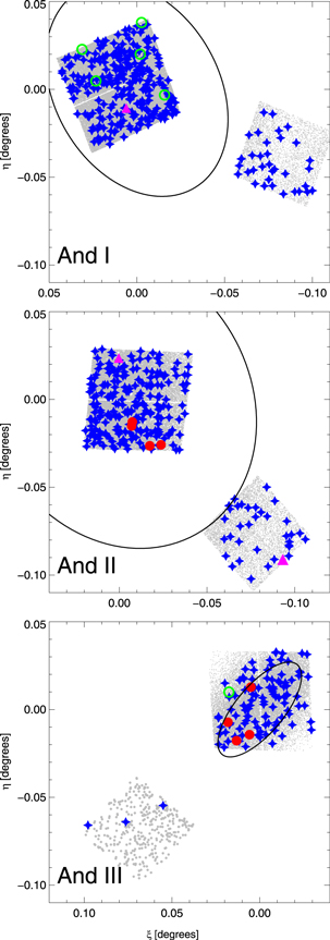
Figure 3. Spatial distribution of the variable stars found in the observed ACS+WFC3 fields for And I, II, and III. Non-variable stars are represented by gray dots. Variables are shown with the same symbol and color code as in Figure 1. The black ellipses represent the half-light radius (rh) for each galaxy (column 6 in Table 1).
Download figure:
Standard image High-resolution image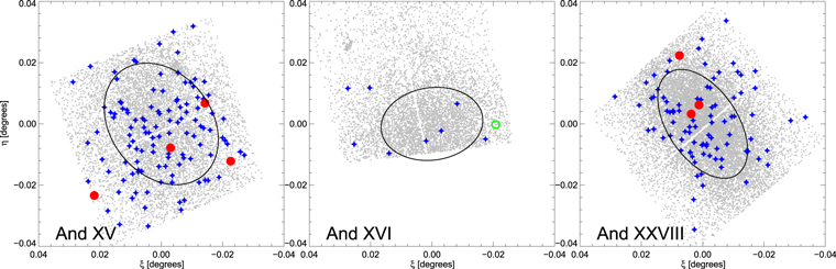
Figure 4. Spatial distribution of the variable stars found in the observed ACS fields for And XV, XVI, and XXVIII. Non-variable stars are represented by gray dots. Variables are shown with the same symbol and color code as in Figure 1. The black ellipses represent the half-light radius (rh) for each galaxy (column 6 in Table 1). The WFC3 fields are not shown here because the CMDs of these three fields do not have any evidence of a satellite stellar population.
Download figure:
Standard image High-resolution image4. RR Lyrae Stars
4.1. Mean Properties and Bailey Diagrams
RRL stars are low-mass (∼0.6–0.8  ) and radially pulsating variable stars with periods ranging from 0.2 to 1.0 day and V amplitudes from 0.2 to ≲2 mag. They are found in stellar systems that host an old (t > 10 Gyr) stellar population (Walker 1989; Smith 1995; Catelan & Smith 2015). A total of 870 RRL stars were detected and characterized in the six ISLAndS galaxies. Table 4 summarizes for each galaxy, the number of fundamental (RRab), first-overtone (RRc), and double-mode (RRd) pulsators in both the ACS and WFC3 fields of view. Different types of RRL stars are usually easy to classify on the basis of a visual inspection of the LC and the period. RRab stars are characterized by longer periods (∼0.45–1.0 days) and saw-tooth LCs, with a steep rise up to the maximum and a less steep fall to the minimum. RRc have shorter periods (∼0.2–0.45 days), lower amplitudes (
 ), and almost sinusoidal light variations. Conversely, RRd stars usually have periods around 0.4 day, and their LCs are particularly noisy due to simultaneous pulsation in the fundamental mode and first overtone. Figure 5 presents an example RRL LC for each galaxy. Black and gray points are used for data in the
  and
and  passbands, respectively. Open symbols are used to indicate outlier measurements that have not been taken into account in deriving the pulsational properties. We emphasize that the whole set of LCs is available in the electronic edition of this paper. Additionally, the properties of the individual variable stars can be found in Appendix D.
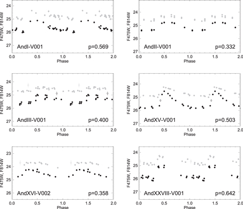
Figure 5.
Examples of LCs of member RRL stars from each of the six ISLAndS galaxies in the  (black) and
  (gray) bands. Periods (in days) are given in the lower right corner, while the name of the variable is displayed at the left-hand side of each panel. Open symbols show the data-points for which the uncertainties are larger than 3σ above the mean error of a given star; these data were not used in period and mean-magnitude calculations. The total set of LCs for all the RRL stars found in each galaxy of this work is available in the online journal. (The complete figure set (61 images) is available.)
Download figure:
Standard image High-resolution imageTable 4. RRL Star Subgroups
| And I | And II | And III | And XV | And XVI | And XXVIII | Total | ||
|---|---|---|---|---|---|---|---|---|
| ACS | 203 | 160 | 83 | 80 | 3 | 35 | 562 | |
| RRab | WFC3 | 26 | 27 | 1 | 0 | 0 | 0 | 53 |
| total | 229 | 187 | 84 | 80 | 3 | 35 | 615 | |
| ACS | 42 | 42 | 13 | 24 | 5 | 35 | 158 | |
| RRc | WFC3 | 6 | 6 | 2 | 0 | 0 | 0 | 14 |
| total | 48 | 48 | 15 | 24 | 5 | 34 | 172 | |
| ACS | 16 | 15 | 12 | 13 | 0 | 15 | 69 | |
| RRd | WFC3 | 3 | 1 | 0 | 0 | 0 | 0 | 4 |
| total | 19 | 16 | 12 | 13 | 0 | 15 | 73 | |
| TOTALACS | 261 | 217 | 108 | 117 | 8 | 85a | 797 | |
| TOTALWFC3 | 35 | 34 | 3 | 0 | 0 | 0 | 72 | |
| TOTAL | 296 | 251 | 111 | 117 | 8 | 85a | 869 | |
Note.
aWe have identified two additional RRL star candidates with noisy LCs. We do not include them here because of the uncertainty in their classification.Download table as: ASCIITypeset image
Figure 6 presents the period–amplitude (Bailey) diagram for the six galaxies (see caption for details). The plot shows the two different relations for the Oosterhoff types, represented in the plot by the dashed lines (Oosterhoff I and II, or Oo-I and Oo-II Cacciari et al. 2005). As has long been known (Oosterhoff 1939, 1944), the properties of RRab stars divide Galactic GCs into two groups, called Oosterhoff I and Oosteroff II. The mean period of fundamental pulsators of the former group is shorter (P ∼ 0.55 day) than in the latter (P ∼ 0.65). Although the origin of this behavior has not been fully explained, the Oosterhoff dichotomy appears to be related to the metallicity of the clusters, where the Oo-II stars are more metal-poor, on average (e.g., see the review by Catelan 2009). On the other hand, dwarf galaxies do not show a similar behavior, as the mean period of their RRab stars typically locates them in the Oosterhoff gap between the two Oostherhoof groups. For this reason, they have often been considered as Oosterhoff-intermediate types (see e.g., Kuehn et al. 2008; Bernard et al. 2009, 2010; Garofalo et al. 2013; Stetson et al. 2014; Cusano et al. 2015; Ordoñez & Sarajedini 2016).
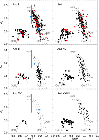
Figure 6. Period–amplitude or Bailey diagrams for the RRL samples. Stars and circles represent RRab and RRc stars (respectively) found in the ACS field (black) and in the WFC3 (red). Blue squares show the five RRLs that are probable M31 field stars. The dashed gray lines are the relations for RRab stars in Oo-I and Oo-II clusters obtained by Cacciari et al. (2005), while the dotted gray line delimits the middle position between the last two. The gray solid curve is derived from the M22 (Oo-II cluster) RRc stars by Kunder et al. (2013). Gray vertical lines mark the HASP limit defined by Fiorentino et al. (2015) (see text for further details). For the sake of clarity, RRd stars are not plotted.
Download figure:
Standard image High-resolution imageTable 5 summarizes the mean pulsational properties for the galaxies in our sample: the mean periods of RRab-type ( ) and RRc-type (
 ) stars, the fraction of RRc (fc) and of RRc+RRd (fcd) stars, the fraction of Oo-I-like and Oo-II-like stars (defined below in this section), and the apparent mean magnitude in V band (which we use in Section 6 to determine the distance to the galaxy). From the information in the table, the six ISLAndS galaxies could also be considered Oosterhoff-intermediate, since they have
  day. In this respect, the ISLAndS galaxies are similar to the MW dSph satellites. However, an intermediate mean period does not mean that the stars are distributed in the Bailey diagram between the two typical Oosterhoff lines. Figure 6 clearly shows that stars tend to clump around each Oosterhoff group locus, and with a predominance of Oo-I like stars. In fact, if we split the sample using the dotted intermediate line and classify stars as Oo-I like or Oo-II like according to their relative position with respect to this separator, four galaxies (And I, II, III, and XV) present a majority (∼80%) of Oo-I like stars (see Table 6). In the case of And I and II, the same result was found for the variable stars in the parallel WFC3.
Table 5. Mean Properties of the RRL Stars
| Galaxy |

|

|
fc | fcd | % Oo-I | % Oo-II |

|
|---|---|---|---|---|---|---|---|
| And I | 0.597 ± 0.004 (σ = 0.07) | 0.343 ± 0.005 (σ = 0.03) | 0.17 | 0.23 | 80 | 20 | 25.13 |
| And II | 0.601 ± 0.005 (σ = 0.07) | 0.332 ± 0.006 (σ = 0.04) | 0.20 | 0.25 | 80 | 20 | 24.78 |
| And III | 0.622 ± 0.004 (σ = 0.03) | 0.344 ± 0.011 (σ = 0.04) | 0.15 | 0.24 | 89 | 11 | 25.04 |
| And XV | 0.608 ± 0.006 (σ = 0.05) | 0.360 ± 0.009 (σ = 0.04) | 0.23 | 0.32 | 78 | 22 | 25.07 |
| And XVI | 0.636 ± 0.010 (σ = 0.02) | 0.356 ± 0.019 (σ = 0.04) | ⋯ | ⋯ | 67 | 33 | 24.34 |
| And XXVIII | 0.624 ± 0.012 (σ = 0.07) | 0.359 ± 0.007 (σ = 0.04) | 0.50 | 0.59 | 49 | 51 | 25.14 |
Note. Mean periods are given in days. The definition of fc is  , while fcd is defined as
  .
.
Download table as: ASCIITypeset image
Table 6. Properties of the Set of RRL Stars in a Sample of 41 LG Dwarf Galaxies of Different Morphological Type within ∼2 Mpc, with at Least Five RRab and with Data Available in the Literature
| RRab |

|

|
|||||||||
|---|---|---|---|---|---|---|---|---|---|---|---|
| Galaxy |
![$\langle [\mathrm{Fe}/{\rm{H}}]\rangle $](https://content.cld.iop.org/journals/0004-637X/850/2/137/revision1/apjaa9381ieqn218.gif) a
a
|
RRab | %OoI | %OoII | RRcd | fcd | Median | Mean | Median | Mean | References |
| MW dwarf satellites | |||||||||||
| Ursa Major I | −2.18 | 5 | 60 | 40 | 2 | 0.29 | 0.600 | 0.628 ± 0.031(0.07) | 0.407 | 0.402 ± 0.005(0.008) | Garofalo et al. (2013) |
| Bootes I | −2.55 | 7 | 43 | 57 | 8 | 0.53 | 0.680 | 0.691 ± 0.034(0.09) | 0.386 | 0.364 ± 0.016(0.04) | Siegel (2006) |
| Hercules | −2.41 | 6 | 0 | 100 | 3 | 0.33 | 0.678 | 0.678 ± 0.013(0.03) | 0.400 | 0.399 ± 0.002(0.003) | Musella et al. (2012) |
| Canes Venatici I | −1.98 | 18 | 72 | 28 | 5 | 0.22 | 0.610 | 0.604 ± 0.006(0.03) | 0.390 | 0.378 ± 0.012(0.03) | Kuehn et al. (2008) |
| Draco | −1.93 | 211 | 87 | 13 | 56 | 0.21 | 0.608 | 0.615 ± 0.003(0.04) | 0.401 | 0.389 ± 0.004(0.03) | Kinemuchi et al. (2008) |
| Ursa Minor | −2.13 | 47 | 45 | 55 | 35 | 0.43 | 0.648 | 0.638 ± 0.009(0.06) | 0.383 | 0.375 ± 0.011(0.07) | Nemec et al. (1988) |
| Carina | −1.72 | 71 | 73 | 27 | 12 | 0.15 | 0.630 | 0.634 ± 0.005(0.05) | 0.364 | 0.350 ± 0.013(0.04) | Coppola et al. (2015) |
| Sextans | −1.93 | 26 | 62 | 38 | 10 | 0.28 | 0.596 | 0.606 ± 0.010(0.05) | 0.352 | 0.355 ± 0.019(0.06) | Mateo et al. (1995) |
| Leo II | −1.62 | 106 | 63 | 37 | 34 | 0.24 | 0.615 | 0.619 ± 0.006(0.06) | 0.370 | 0.363 ± 0.008(0.05) | Siegel & Majewski (2000) |
| Sculptor | −1.68 | 289 | 56 | 44 | 247 | 0.46 | 0.593 | 0.610 ± 0.006(0.10) | 0.355 | 0.346 ± 0.002(0.04) | Martínez-Vázquez et al. (2016b) |
| Leo I | −1.43 | 136 | 74 | 26 | 28 | 0.17 | 0.591 | 0.599 ± 0.005(0.06) | 0.367 | 0.352 ± 0.007(0.04) | Stetson et al. (2014) |
| Fornax | −0.99 | 998 | 84 | 16 | 445 | 0.31 | 0.594 | 0.595 ± 0.001(0.05) | 0.380 | 0.379 ± 0.001(0.07) | Fiorentino et al. (2017) |
| Sagittarius | −0.40 | 1636 | 79 | 21 | 409 | 0.20 | 0.576 | 0.575 ± 0.002(0.07) | 0.322 | 0.319 ± 0.002(0.04) | Soszyński et al. (2014) |
| SMC | −1.00 | 4961 | 83 | 17 | 1407 | 0.22 | 0.598 | 0.598 ± 0.0008(0.06) | 0.366 | 0.360 ± 0.001(0.04) | Soszyński et al. (2016) |
| LMC | −0.50 | 27620 | 75 | 25 | 11461 | 0.29 | 0.576 | 0.580 ± 0.0004(0.07) | 0.339 | 0.333 ± 0.000(0.04) | Soszyński et al. (2016) |
| M31 dwarf satellites | |||||||||||
| And XIII | −1.90 | 8 | 63 | 37 | 1 | 0.11 | 0.616 | 0.648 ± 0.026(0.07) | 0.4287 | 0.4287 | Yang & Sarajedini (2012) |
| And XI | −2.00 | 10 | 70 | 30 | 5 | 0.33 | 0.626 | 0.621 ± 0.026(0.08) | 0.428 | 0.423 ± 0.013(0.03) | Yang & Sarajedini (2012) |
| And XXVIII | −1.73 | 35 | 49 | 51 | 50 | 0.59 | 0.622 | 0.624 ± 0.012(0.07) | 0.366 | 0.361 ± 0.005(0.04) | This work |
| And XVI | −1.91 | 3 | 67 | 33 | 5 | 0.63 | 0.640 | 0.636 ± 0.010(0.02) | 0.358 | 0.356 ± 0.019(0.04) | This work |
| And XIX | −1.80 | 23 | 44 | 56 | 8 | 0.26 | 0.616 | 0.618 ± 0.007(0.03) | 0.401 | 0.392 ± 0.010(0.03) | Cusano et al. (2013) |
| And XV | −1.80 | 80 | 76 | 22 | 37 | 0.32 | 0.608 | 0.608 ± 0.006(0.05) | 0.366 | 0.364 ± 0.006(0.04) | This work |
| And XXV | −1.80 | 45 | 67 | 33 | 11 | 0.20 | 0.608 | 0.607 ± 0.007(0.05) | 0.370 | 0.363 ± 0.010(0.03) | Cusano et al. (2016) |
| And XXI | −1.80 | 37 | 49 | 51 | 4 | 0.10 | 0.619 | 0.638 ± 0.010(0.06) | 0.387 | 0.343 ± 0.028(0.06) | Cusano et al. (2015) |
| And III | −1.81 | 84 | 89 | 11 | 27 | 0.24 | 0.620 | 0.623 ± 0.004(0.03) | 0.375 | 0.375 ± 0.012(0.06) | This work |
| And VI | −1.30 | 91 | 87 | 13 | 20 | 0.18 | 0.587 | 0.588 ± 0.006(0.05) | 0.386 | 0.382 ± 0.009(0.04) | Pritzl et al. (2002) |
| And I | −1.44 | 229 | 80 | 20 | 67 | 0.23 | 0.588 | 0.597 ± 0.004(0.07) | 0.353 | 0.349 ± 0.004(0.03) | This work |
| And II | −1.30 | 187 | 80 | 20 | 64 | 0.26 | 0.600 | 0.601 ± 0.005(0.07) | 0.350 | 0.341 ± 0.005(0.04) | This work |
| And VII | −1.40 | 386 | 75 | 25 | 187 | 0.33 | 0.571 | 0.578 ± 0.003(0.06) | 0.342 | 0.338 ± 0.003(0.04) | Monelli et al. (2017) |
| NGC 147 | −1.10 | 118 | 70 | 30 | 59 | 0.33 | 0.577 | 0.589 ± 0.008(0.09) | 0.331 | 0.325 ± 0.006(0.05) | Monelli et al. (2017) |
| NGC 185 | −1.64 | 544 | 63 | 37 | 276 | 0.34 | 0.580 | 0.587 ± 0.004(0.09) | 0.325 | 0.322 ± 0.003(0.04) | Monelli et al. (2017) |
| M32 | −0.25 | 314 | 80 | 20 | 102 | 0.25 | 0.564 | 0.569 ± 0.005(0.08) | 0.324 | 0.323 ± 0.004(0.04) | Fiorentino et al. (2012) |
| Isolated dwarf galaxies | |||||||||||
| Tucana | −2.00 | 216 | 68 | 32 | 142 | 0.40 | 0.597 | 0.604 ± 0.004(0.06) | 0.370 | 0.367 ± 0.003(0.03) | Bernard et al. (2009) |
| Phoenix | −1.37 | 95 | 70 | 30 | 26 | 0.21 | 0.592 | 0.602 ± 0.007(0.06) | 0.360 | 0.363 ± 0.014(0.07) | Ordoñez et al. (2014) |
| LGS3 | −2.10 | 109 | 69 | 31 | 24 | 0.18 | 0.607 | 0.616 ± 0.007(0.07) | 0.372 | 0.360 ± 0.011(0.05) | C. E. Martínez-Vázquez et al. (2018, in preparation) |
| DDO 210 | −1.30 | 24 | 92 | 8 | 8 | 0.25 | 0.606 | 0.609 ± 0.010(0.05) | 0.374 | 0.359 ± 0.027(0.08) | Ordoñez & Sarajedini (2016) |
| Cetus | −1.90 | 506 | 83 | 17 | 124 | 0.20 | 0.610 | 0.613 ± 0.002(0.04) | 0.389 | 0.381 ± 0.003(0.04) | Monelli et al. (2012) |
| Leo A | −1.40 | 7 | 71 | 29 | 3 | 0.30 | 0.625 | 0.637 ± 0.014(0.04) | 0.372 | 0.366 ± 0.017(0.03) | Bernard et al. (2013) |
| IC1613 | −1.60 | 61 | 64 | 36 | 29 | 0.32 | 0.606 | 0.611 ± 0.010(0.08) | 0.349 | 0.339 ± 0.006(0.03) | Bernard et al. (2010) |
| NGC 6822 | −1.00 | 24 | 83 | 17 | 2 | 0.08 | 0.603 | 0.605 ± 0.007(0.04) | 0.406 | 0.388 ± 0.019(0.03) | Baldacci et al. (2005) |
| Sculptor Group dwarf galaxies | |||||||||||
| ESO410-G005 | −1.93 | 224 | 66 | 34 | 44 | 0.16 | 0.578 | 0.589 ± 0.005(0.07) | 0.327 | 0.317 ± 0.010(0.06) | Yang et al. (2014) |
| ESO294-G010 | −1.48 | 219 | 62 | 38 | 13 | 0.06 | 0.589 | 0.593 ± 0.004(0.06) | 0.345 | 0.330 ± 0.017(0.06) | Yang et al. (2014) |
Note.
aMean metallicity for each galaxy obtained from McConnachie (2012).Download table as: ASCIITypeset image
And XXVIII is the exception, with a fraction of Oo-I like stars close to 50%. Moreover, the distribution of RRLs in the Bailey diagram is also different from the other And dSphs; the RRab stars show a broad spread and are not concentrated on either Oosterhoff line. And XXVIII is also peculiar for the large fraction of RRcd-type stars, which represent ∼58% of the total. In the LG, if we exclude low-mass galaxies with very small samples of RRLs (<15, such as Bootes I and And XVI, see Section 5.2), And XXVIII is the only galaxy with more RRcd-type than RRab-type stars. Similar to And XXVIII, the galaxies with a particularly large fraction of RRcd (Ursa Minor: 43%, Nemec et al. 1988; Sculptor: 46%, Martínez-Vázquez et al. 2016b; Tucana: 40%, Bernard et al. 2009) are all also characterized by the presence of a strong blue HB component. This may be connected to a sizable population of very metal-poor stars.
The black vertical line in Figure 6 marks the limit of the high-amplitude short-period (HASP) region, defined by Fiorentino et al. (2015) as those RRab stars with periods shorter than 0.48 day and amplitudes in the V band larger than 0.75 mag. These stars are interpreted as the metal-rich tail of the metallicity distribution of RRL stars ([Fe/H] > −1.5), and have only been found in systems that were dense or massive enough to enrich to this metallicity before 10 Gyr ago (Fiorentino et al. 2017). We confirm this trend with the six ISLAndS galaxies, as HASPs have only been detected in the two most massive satellite galaxies: And I (3)20 and And II (2). A detailed analysis of the chemical properties of RRL stars will be discussed in a forthcoming paper.
It is worth noting that a few stars with HASP properties were already identified in the catalogs by Pritzl et al. (2004) and Pritzl et al. (2005) for And II and And I, respectively. In the case of And I, we confirm the HASP nature of three out of the seven stars, while the period was likely underestimated for the other four, possibly due to aliasing (see Appendix C). However, we do not confirm any of the eight HASP stars in And II (see Appendix C for a detailed comparison with literature values). Nevertheless, we discovered two new HASPs in And I and two in And II, which are both located outside the WFPC2 field studied by Pritzl et al. (2004, 2005).
4.2. Five Detected RR Lyrae Stars from the M31 GSS
Five RRLs in And I have mean magnitudes that are a few tenths of a magnitude fainter than the HB (three RRab: AndI-V053, AndI-V110 and AndI-V113; and two RRc: AndI-V257 and AndI-V280). We exclude the possibility that sampling problems of the LC may be causing a bias toward fainter magnitudes. Possible explanations are (i) a significantly higher metal content, or (ii) a distance effect. Assuming they are at the distance of And I, in order to explain such a faint luminosity (0.45 mag fainter), a super solar metallicity is required. This value appears to be unlikely given the morphology of the CMD and the SFH (Skillman et al. 2017).
On the other hand, as indicated in the previous section, the CMD of And I shows that a significant contamination by the GSS is present along the line of sight to And I. In particular, And I is projected on the GSS "Field 3" studied by McConnachie et al. (2003), which is located at 860 ± 20 kpc according to the TRGB determination. To verify whether the faint RRL stars can be associated with the GSS, we first note that two of the three RRab are HASP RRL stars. This suggests that their metallicity is likely to be higher than −1.5 dex. Assuming [Fe/H] = −1.5 and using the PWR described in Section 6.2, we obtain a mean distance modulus of  mag (sys = 0.08; rand = 0.11) for the five stars, corresponding to 937 kpc (sys = 34; rand = 47). This means that they are likely located ∼140 kpc beyond And I (
 , see Section 6). Given the error bars, we conclude that the five faint RRL stars are compatible with being connected to the metal-poor component of the GSS (Gilbert et al. 2009) rather than members of And I.
5. Properties of the Old Population in the M31 and MW Satellite Systems
5.1. Comparing the HB Morphologies of the MW and M31 Satellites
Pioneering works by Da Costa et al. (1996, 2000, 2002) based on shallower WFPC2 data disclosed the first hint that the M31 satellites are characterized by a redder HB morphology than MW dwarfs. A similar conclusion was reached by Martin et al. (2017), based on ACS data for 20 M31 galaxies. The analysis was based on a morphological index accounting for the number of blue and red HB stars. In this section we apply a similar approach, and taking advantage of the known number of RRL stars, we can compare the morphology index RHB21 of the six ISLAndS galaxies and of a sample of MW satellites. The latter consists of revised data for Carina, Fornax, Sculptor, Draco, and Leo II from the updated catalogs available in P. B. Stetson's database (P. B. Stetson 2017, private communication). These studies are part of an ongoing series of papers on variable stars in GCs and dwarf galaxies by ourselves and our collaborators (Stetson et al. 2014; Braga et al. 2015, 2016; Coppola et al. 2015; Martínez-Vázquez et al. 2016b; Fiorentino et al. 2017).
The value of the RHB index was calculated in a homogeneous way considering only stars within one half-light radius, rh. This was possible for all of the galaxies except for And I and II, since the ACS only covers a fraction of such area (see Figure 3). In the case of the MW satellites, we estimated and subtracted the Galactic field-star contribution using a proper control field in the outskirts of each object. The exact limits in color and magnitude for the selection of HB stars for the RHB index were defined on a per-galaxy basis because of the variety of CMD morphology, filter bandpasses, and foreground contamination. However, these were carefully chosen to limit contamination from any RGB, AGB, RC, and blue straggler populations present, while also avoiding biases.
Figure 7 shows, as a function of the host galaxy absolute MV magnitude, the RHB index calculated inside 1 rh for the MW (open diamonds) satellites and for the ISLAndS (stars) galaxies. And I and II are calculated over the full ACS area, which is smaller than one rh. The plot suggests that at least in the innermost regions of the available samples, the M31 satellites have slightly redder HBs than the MW dSph satellites, although the difference is within 2σ. In fact, within one rh, the mean value of RHB is more negative in the case of M31 galaxies ( ) than for the MW companions (
 ). However, we emphasize that the latter numbers may be biased due to the small subsample of satellites for which we have data in both MW and M31 systems.
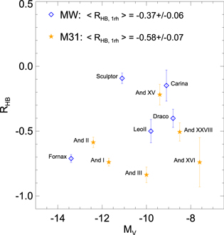
Figure 7. RHB index vs. the luminosity of the host galaxy, MV, for the ISLAndS targets (orange filled stars) and a sample of MW satellites (blue open diamonds). The values have been calculated within one rh, except for And I and II (red stars), since the field of view of the ACS is not large enough. The mean value for M31 satellites supports a redder HB morphology than for MW satellites.
Download figure:
Standard image High-resolution imageIt is worth mentioning that the present analysis presents several improvements over previous analyses (Harbeck et al. 2001; Martin et al. 2017): (i) the better photometric precision at the HB level, and the filter combination, which provides a better color discriminating power. This allows us to clearly separate the red HB from the blue edge of the RGB, even in the case of And I. (ii) The larger field of view of ACS compared to WFPC2 provided a larger sample. (iii) The up-to-date wide-field homogeneous data available for the MW companions allowed us to perform the comparison in a more homogeneous manner. (iv) Finally, the better phase coverage allowed us to derive better-defined mean colors of RRL stars.
The current data do not allow us to fully explore whether the HB morphology presents significant variation as a function of galactocentric distance, i.e., distance from the center of each galaxy. Nevertheless, when considering the parallel WFC3 field for And I and And II, we derive higher values of the RHB index, and therefore an indication that the HB morphology becomes bluer when moving to an external region. This is in agreement with what has been found for other LG galaxies (e.g., Harbeck et al. 2001; Tolstoy et al. 2004; Cole et al. 2017), and more in general, with the population gradients commonly found in dwarf galaxies (Hidalgo et al. 2013, and references therein). In fact, when considering the area within two rh, the six galaxies tend to have bluer HB. Unfortunately, a straight comparison between the two satellite systems is complicated by the fraction of area covered. This leaves open the question whether the HB morphology remains different at larger galactocentric distances, or if M31 and MW satellites tend to be more similar when their global properties are taken into account. More wide-field variability studies, particularly for the M31 satellites, would help solve this problem.
5.2. Global Properties of RRL Stars
In Section 4 we presented the Bailey diagram of the ISLAndS galaxies and discussed their properties in terms of Oosterhoff classification. Despite the intermediate mean-period, stars in the Bailey diagram still tend to clump around the Oo-type lines, with a predominance of Oo-I-like stars, rather than in between. Therefore, the period distribution provides a more detailed description than the mean period alone (Fiorentino et al. 2015, 2017). In the previous subsection, we have presented evidence that M31 and MW satellites present a slightly different HB morphology. We now focus on the properties of the RRL stars alone.
Table 6 lists the properties of the RRL in a sample of 41 dwarf galaxies (39 LG dwarfs plus 2 Sculptor group dwarfs) of different morphological type within 2 Mpc (column 1): the number of RRab stars (column 2), the percent of Oo-I type and Oo-II type RRab stars (column 3 and 4), the number of RRcd stars (column 5), the fraction of RRcd stars over the total of the RRL (column 6), and the median and mean period of the RRab and RRcd stars (column 7, 8, 9, and 10) derived from the literature (references in column 11).
The left panel of Figure 8 shows the mean period of RRab-type stars,  , as a function of the mean metallicity of the host galaxy (left panel), for 16 satellites of M31 (filled orange stars) and 15 MW dwarfs (blue open diamonds). Galaxies with at least 5 known RRab stars have been included. The plot discloses that the mean period of RRab-type stars decreases for increasing mean metallicity of the host system (Sandage et al. 1981), for both the MW and the M31 satellites. The trend presents some scatter, but interestingly, a linear fit to the data provides a very similar slope (0.040 ± 0.008 and 0.038 ± 0.008, respectively), thus suggesting an overall similar behavior in the two satellite systems.
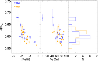
Figure 8. Left and middle panel: mean period of the RRab stars of the sample of MW (blue) and M31 (orange) satellites vs. the mean metallicity and the percentage of Oo-I type stars in the system. There is no obvious difference between the two subgroups. Right panel: mean period distribution of the sample of MW (blue histogram) and M31 dwarf galaxies (orange histogram). The peaks of the two distribution are very close to each other.
Download figure:
Standard image High-resolution imageThe decreasing mean period for increasing metallicity can be related to the early chemical evolution of the sample galaxies. On the one hand, the distribution of stars in the Bailey diagram suggests that galaxies tend to progressively populate the RRab short-period range for increasing metallicity (and mass). This translates into a shorter mean period. It may appear intriguing that a property of a purely old stellar tracer correlates with the present-day mean metallicity of the host galaxy. This suggests that galaxies that today are more massive and more metal-rich on average also experienced faster early chemical evolution, which is imprinted in the properties of their RRL stars. This implies that the mass–metallicity relation (e.g., Kirby et al. 2013) was in place at early epoch (Martínez-Vázquez et al. 2016b).
The central panel of Figure 8 shows the mean period as a function of the fraction of Oo-I type stars, as defined in Section 4. While there is no clear correlation for either satellite system, we find that the vast majority of galaxies host a larger fraction of Oo-I type stars, between 60% and 90% of the total amount of RRab stars. Nevertheless, the mean period of fundamental pulsators would classify them as Oo-intermediate system. Again, this suggests that the RRL stars in complex systems such as galaxies are not properly represented by a single parameter.
Finally, the right panel of Figure 8 shows the mean period distribution for the RRab in MW satellites (blue) and in M31 satellites (orange). Apparently, the two are similar, and their peaks agree within 1σ.
This analysis reveals that if we limit the comparison to strictly old and well-defined populations such as that of RRL stars, there are no obvious differences between the RRL populations of the satellite systems of M31 and the MW.
Figure 9 shows the behavior of  versus [Fe/H], but comparing a sample of 41 galaxies (black circles, including MW and M31 satellites, isolated dwarfs, and 2 galaxies in the Sculptor group) with GCs (magenta bowtie symbols). We use here the compilation from Catelan (2009), including all the GCs with more than 10 RRL stars. Galactic GCs are shown together with clusters from the LMC and the Fornax dSph galaxy. The plot shows that a few Oo-intermediate clusters overlap with galaxies in the Oosterhoff gap, but most of the Oo-I clusters (i.e., with
  ) occupy a region of the parameter space where no galaxies are present—this holds even when we restrict the GC sample to those with 30 RRL or more. This is even more evident in the right panel of Figure 9, which shows the mean period distributions of the two samples. It clearly shows that the peak for the galaxy distribution occurs at a period typical of Oo-intermediate systems, while the peak of the GCs occurs in the Oo-I regime.
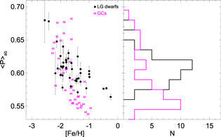
Figure 9. Left panel:  for a sample of 41 dwarf galaxies reported in Table 6 (black dots) as a function of [Fe/H], compared to that of GCs (purple bowties). Right panel: period distribution of the sample of dwarf galaxies and GCs. The peak of the former occurs at a period typical of the Oo-intermediate system, while the latter peaks in the short-period regime, populated by Oo-I systems, which is devoid of galaxies.
Download figure:
Standard image High-resolution image6. Distance Moduli
In the following, we use four independent methods to derive the distances to the six ISLAndS galaxies, the first three based on the properties of the RRL stars: (i) the reddening-free PWRs (Marconi et al. 2015); (ii) the luminosity–metallicity (MV versus [Fe/H]) relation (LMR, Bono et al. 2003; Clementini et al. 2003); and (iii) the first-overtone blue-edge (FOBE) relation (Caputo et al. 2000); these are supplemented by (iv) the TRGB method.
All these relations require an assumption for the metal abundance. In particular, in the case of the PWR, LMR, and FOBE relation, we need to assume a metallicity corresponding to the old population (representative of the RRL stars). On the other hand, the TRGB method uses the metallicity of the RGB stars to obtain the expected mean color value of the TRGB. In complex systems like dwarf galaxies, the metallicity of the global population may range over ∼2 dex, and in many systems, a mix of old and intermediate-age populations is present. However, the metallicity adopted for the methods based on RRL stars must be representative of the old stellar population. In the next section, we discuss the choice of the metallicity in detail in order to determine the distance to the six galaxies.
6.1. The Choice of the Metallicity
The metallicity estimates available in the literature for the ISLAndS galaxies are all based on CaT spectroscopy of bright RGB stars.22 As the RGB can be populated by stars of any age older than ∼1 Gyr, the derived metallicity distribution may not be representative of the RRL stars, since relatively young and/or more metal-rich populations may exist on the RGB, but may not have counterparts among RRL stars (Martínez-Vázquez et al. 2016a). As a consequence, assuming a mean metallicity that may be too high by 1.0 dex for the RRL stars would introduce a systematic error in the distance modulus estimates at the level of ∼0.2 mag.
Table 7 lists literature values for the mean metallicity (column 2) of ISLAndS galaxies, the σ of the metallicity distribution (column 3), and the number of RGB stars (column 4) used in these studies (references in column 5). Relatively low values were found for And III, And XV, And XVI, and And XXVIII, on average close to [Fe/H] ∼ −1.8 or lower. On the other hand, in the case of And I and And II, different authors (Kalirai et al. 2010; Ho et al. 2012) agree on a much higher mean metallicity ([Fe/H] ∼ −1.4), and a relatively large metallicity spread ( dex,
dex,  dex). Nevertheless, the small number of HASP stars (see Section 4) suggests that even if the tail of the RRL metallicity distribution reaches such relatively high values, the bulk of the RRL stars must have a lower metallicity ([Fe/H] < –1.5, Fiorentino et al. 2015). Therefore, as representative values of the metallicity for the RRL population, we adopted—in agreement with their SFHs (Skillman et al. 2017)—[Fe/H] = –1.8 for And I and And II, while for the rest of the galaxies, we assumed that the metallicity of the old population must be quite similar to that obtained by the spectroscopic studies (see column 8).
Table 7. Metallicity Studies with the Largest Samples of RGB Stars
| RGB stars | RRL Stars | ||||||
|---|---|---|---|---|---|---|---|
| Galaxy |
![$\langle [\mathrm{Fe}/{\rm{H}}]\rangle $](https://content.cld.iop.org/journals/0004-637X/850/2/137/revision1/apjaa9381ieqn229.gif)
|
![${\sigma }_{\langle [\mathrm{Fe}/{\rm{H}}]}\rangle $](https://content.cld.iop.org/journals/0004-637X/850/2/137/revision1/apjaa9381ieqn230.gif)
|
Nstars | References | Metallicity Scalea |
![$\langle [\mathrm{Fe}/{\rm{H}}]{\rangle }_{{\rm{C}}09}$](https://content.cld.iop.org/journals/0004-637X/850/2/137/revision1/apjaa9381ieqn231.gif) b
b
|
![${[\mathrm{Fe}/{\rm{H}}]}_{\mathrm{old}\mathrm{pop}.}$](https://content.cld.iop.org/journals/0004-637X/850/2/137/revision1/apjaa9381ieqn232.gif)
|
| And I | −1.45 ± 0.04 | 0.37 | 80 | Kalirai et al. (2010) | ZW84 | −1.44 | −1.8 |
| And II | −1.39 ± 0.03 | 0.72 | 477 | Ho et al. (2012) | G07 | −1.30 | −1.8 |
| And III | −1.78 ± 0.04 | 0.27 | 43 | Kalirai et al. (2010) | ZW84 | −1.81 | −1.8 |
| And XV | −1.80 ± 0.20 | ⋯c | 13 | Letarte et al. (2009) | C09 | −1.80 | −1.8 |
| And XVI | −2.00 ± 0.10 | ⋯d | 12 | Collins et al. (2015) | G07 | −1.91 | −2.0 |
| And XXVIII | −1.84 ± 0.15 | 0.65e | 13 | Slater et al. (2015) | C09 | −1.84 | −1.8 |
Notes.
aMetallicity scales: ZW84—Zinn & West (1984), G07—Grevesse et al. (2007), and C09—Carretta et al. (2009). bWe have either converted the metallicity into the C09 scale when possible or shifted the metallicity value assuming the same solar iron abundance (log(Fe) = 7.54). The C09 scale was chosen as the homogeneous scale because it is the most recent scale.
cLetarte et al. (2009) did not publish ![${\sigma }_{[\mathrm{Fe}/{\rm{H}}]}$](https://content.cld.iop.org/journals/0004-637X/850/2/137/revision1/apjaa9381ieqn233.gif) . Instead, they provide an interquartile range of 0.08, with a median metallicity of [Fe/H] = –1.58 dex.
dCollins et al. (2015) did not publish
. Instead, they provide an interquartile range of 0.08, with a median metallicity of [Fe/H] = –1.58 dex.
dCollins et al. (2015) did not publish ![${\sigma }_{[\mathrm{Fe}/{\rm{H}}]}$](https://content.cld.iop.org/journals/0004-637X/850/2/137/revision1/apjaa9381ieqn234.gif) . However, Letarte et al. (2009) published for And XVI an interquartile range of 0.12, with a median of [Fe/H] = –2.23 dex. By stacking the spectra of the member stars (eight, in this case), they found [Fe/H] = –2.1 with an uncertainty of ∼0.2 dex. This value agrees with that obtained by Collins et al. (2015) (shown in the table).
eAs this σ is obtained from a small number of individual measurements, it may not be representative of the actual distribution.
. However, Letarte et al. (2009) published for And XVI an interquartile range of 0.12, with a median of [Fe/H] = –2.23 dex. By stacking the spectra of the member stars (eight, in this case), they found [Fe/H] = –2.1 with an uncertainty of ∼0.2 dex. This value agrees with that obtained by Collins et al. (2015) (shown in the table).
eAs this σ is obtained from a small number of individual measurements, it may not be representative of the actual distribution.
Download table as: ASCIITypeset image
The adopted mean metallicities for each ISLAndS galaxy are summarized in the penultimate column of Table 7. We note that the values have been homogenized to the scale of Carretta et al. (2009). Column 2 reports the value in the original scale, which is specified in column 6. In the cases that are based on theoretical spectra, we applied a correction to take into account the different solar iron abundance (from  to 7.54), which translates into a distance modulus change between 0.01 mag in the case of the FOBE and 0.04 in the case of the LMR.
6.2. The Period-Wesenheit Relations
PWRs are a powerful tool for distance determination, because they are reddening-free by construction and are only marginally metallicity dependent. They are theoretically described by

where X and Y are magnitudes and W( –Y) denotes the reddening-free Wesenheit magnitude (Madore 1982) obtained as W(
 ) = X–R(X–Y), where R is the ratio of total-to-selective absorption, R = AX/E(X–Y).
An updated and very detailed analysis of the framework of the PWRs is provided by Marconi et al. (2015). Their Tables 7 and 8 give a broad range of optical, optical-NIR, and NIR PWRs, along with their corresponding uncertainties. In particular, in this work, we use their PWR in the ( ) filter combinations23
:
) filter combinations23
:
which has an intrinsic dispersion of σ = 0.04 mag. For this relation, a metallicity change of 0.2 dex translates into a change in the distance on the order of 0.03 mag.
The theoretical W( –I) was obtained from the individual stars assuming a metallicity for the old population (see column 8 in Table 7 and the discussion of Section 6.1). We next calculated the individual apparent Wesenheit magnitude as: w(
 –I) = I–0.78(B–I). We report the distance moduli obtained by averaging individual estimates for the global sample (RRab + fundamentalized RRc: log Pfund = log PRRc + 0.127; Bono et al. 2001) in columnn 2 of Table 8. For comparison, if we independently use the sample of RRab and RRc, the values from the different determinations agree on average within ±0.04 mag. Column 2 of Table 8 reports the true distance moduli obtained for each galaxy using this method.
Table 8.
Summary of the Different True Distance Moduli ( ) Obtained Using Several Methods
| RRL Stars | RGB Stars | ||||||
|---|---|---|---|---|---|---|---|
| Galaxy | PWR | LMRB03 | LMRC03 | FOBEa | TipR07 | TipB11 | TipBaSTI |
| And I | 24.49 ± 0.08(0.11) | 24.54 ± 0.16(0.10) | 24.50 ± 0.14(0.10) | 24.49 ± 0.10 | 24.52 ± 0.11(0.09) | 24.49 ± 0.12(0.09) | 24.56 ± 0.04(0.09) |
| And II | 24.16 ± 0.08(0.10) | 24.15 ± 0.16(0.09) | 24.11 ± 0.14(0.09) | 23.95 ± 0.10 | 24.10 ± 0.11(0.12) | 24.08 ± 0.12(0.12) | 24.17 ± 0.04(0.12) |
| And III | 24.36 ± 0.08(0.08) | 24.44 ± 0.16(0.08) | 24.41 ± 0.14(0.08) | 24.48 ± 0.10 | 24.35 ± 0.11(0.19) | 24.30 ± 0.12(0.19) | 24.37 ± 0.04(0.19) |
| And XV | 24.42 ± 0.08(0.09) | 24.50 ± 0.16(0.07) | 24.47 ± 0.14(0.07) | 24.45 ± 0.10 | ⋯ | ⋯ | ⋯ |
| And XVI | 23.70 ± 0.08(0.09) | 23.73 ± 0.16(0.07) | 23.70 ± 0.14(0.07) | 23.75 ± 0.10 | ⋯ | ⋯ | ⋯ |
| And XXVIII | 24.43 ± 0.08(0.07) | 24.45 ± 0.16(0.08) | 24.42 ± 0.14(0.08) | 24.41 ± 0.10 | ⋯ | ⋯ | ⋯ |
Notes. Systematic uncertainties of each estimation are given without parenthesis, while the random uncertainties are bracketed. The uncertainties include the contribution from a possible metallicity dispersion of 0.3 dex.
aThe FOBE method is based on only one RRc star, for this reason, the values in this column do not have a standard deviation.Download table as: ASCIITypeset image
6.3. The Luminosity–Metallicity Relation
The LMR is another simple, widely used approach to determine distances, in this case, using the mean V magnitude of RRL stars. Although both theoretical and empirical calibrations suggest that the relation is not linear (it is steeper in the more metal-rich regime (see e.g., Caputo et al. 2000; Sandage & Tammann 2006; Cassisi & Salaris 2013 and references therein)), most examples in the literature use one of the different linear relations proposed.
In the present work, we adopted the following relations:

from Clementini et al. (2003) and

The latter is valid only for a metallicity lower than [Fe/H] = –1.6, which is appropriate for the six ISLAndS galaxies (where the metallicity of the old population is considered to be [Fe/H] = –1.8 or lower). Columns 3 and 4 of Table 8 show the true distance moduli obtained using the two relations. They are in excellent agreement with each other and with those derived previously using the PWR.
6.4. The FOBE Method
Another method that can be used to estimate the distance is based on the predicted period–luminosity–metallicity relation for pulsators located along the FOBE of the IS (see Caputo et al. 2000):
which has an intrinsic dispersion of  mag.
mag.
This is considered a particularly robust technique for stellar systems with significant numbers of first-overtone RRL (RRc) stars, especially if the blue side of the IS is well populated. Thus, it can be applied safely to five of our six galaxies25 (see Figure 6). The distance modulus is derived by matching the observed distribution of RRc stars to Equation (5). That is, for a given metallicity and a mass corresponding to the typical effective temperature for RRL stars, we shift the relation until the FOBE matches the observed distribution of RRc stars.
For the adopted metallicity listed in Table 7 and using the evolutionary models from BaSTI (Pietrinferni et al. 2004), we obtain masses at log  of M ∼ 0.7
  . True distance moduli obtained for each galaxy using this method are shown in column 5 of Table 8, and are in good agreement with those described in the previous section.
6.5. The Tip of the RGB
It is well established that the TRGB is a good standard candle thanks to its weak dependence on age (Salaris et al. 2002), and in the I band in particular, on the metallicity (at least for relatively metal-poor systems; Da Costa & Armandroff 1990; Lee et al. 1993). The TRGB is frequently used to obtain reliable distance estimates to galaxies of all morphological types in the LG and beyond (e.g., Rizzi et al. 2007; Bellazzini et al. 2011; Wu et al. 2014). However, determining the cutoff in the luminosity function at the bright end of the RGB is not straightforward in low-mass systems because more than about 100 stars populating the top magnitude of the RGB are required to reliably derive the location of the tip (Madore & Freedman 1995; Bellazzini et al. 2002; Bellazzini 2008). This condition is fulfilled only in And I (>200), And II (>150), and nearly so in And III (∼90). The low number of stars in the other three galaxies prevents us from deriving a reliable measurement of the apparent magnitude of the TRGB.
We applied the same method from Bernard et al. (2013) to determine the magnitude of the TRGB. We convolved the  luminosity functions with a Sobel kernel of the form [1, 2, 0, 2, 1]. From the filter response function, we obtain the center of the peak corresponding to the TRGB of each galaxy:
  ,
,  , and
, and  mag, where the uncertainty is the Gaussian rms width of the peak of the Sobel filter response.
The distances were obtained from the TRGB magnitudes using three calibrations:
(i) the empirical calibrations in the HST flight bands from Rizzi et al. (2007, R07):
(ii) the empirical calibration reported in Bellazzini (2011, B11), derived by Bellazzini (2008) from the original calibration as a function of [Fe/H] obtained in Bellazzini et al. (2001) and revised in Bellazzini et al. (2004):
(iii) the theoretical calibration  , as a function of the color (
 –
– )0, obtained in this work by fitting the BaSTI predictions (Pietrinferni et al. 2004, 2006) for the TRGB brightness for an old (∼12 Gyr) stellar population, a wide metallicity range, and an α-enhanced heavy-element distribution:26
In the case of the Rizzi et al. (2007) calibration, we considered that  –
– ∼V–I.27
In fact, for both this calibration and that of Bellazzini et al. (2011), we used the following equation to determine the expected (V–I)0 color: (V–I)
∼V–I.27
In fact, for both this calibration and that of Bellazzini et al. (2011), we used the following equation to determine the expected (V–I)0 color: (V–I) [Fe/H]2+2.472[Fe/H]+4.013 (Bellazzini et al. 2001). Since this last equation is based on the Zinn & West (1984, ZW84) scale, in order to use it properly, we have to apply the conversion scales provided by Carretta et al. (2009): [Fe/H]ZW84 = ([Fe/H]C09–0.160)/1.105. Columns 6, 7, and 8 in Table 8 give the values of the true distance moduli calculated using the previous relations for And I, And II, and And III. All three calibrations lead to distances that are in good agreement with each other and with the previously calculated RRL-based distances.
6.6. On the Consistency of the Different Methods
As show in Table 8, all the distances obtained from the different methods are in agreement within less than 1σ with each other. The inclusion of the TRGB method in this study was mainly to check the distances we obtained using the properties of the RRL stars with those assessed with this method. In fact, it is worth mentioning that since the TRGBs of these galaxies are not densely populated (we have ≳200 only for And I), this technique is secondary in our study, but it serves to show that the metallicity we have assumed for the old population is robust. The good sampling of our LCs together with the large amount of RRL stars in all these galaxies (with exception of And XVI) make them the best distance indicators that we have in these galaxies so far.
We adopt the distances obtained with the PWR as preferred because (i) they are obtained with the RRL stars, (ii) the PWR used to derive them come from the most recently updated study (Marconi et al. 2015), and (iii) the systematic uncertainties are the smallest (see Table 8).
Figure 10 summarizes the distance determinations derived in this work. In particular, the filled circles together with the dotted line show the adopted final distance measurement coming from the PWR (Section 6.2). Open circles show the results from the RRL-based methods presented in previous sections (see Table 8), while the open squares show the TRGB distances. The plot shows that the agreement between the different methods presented here is remarkably good, as most of the derived distances agree within 1σ. Taking as reference the PWR distance, some general trends can be noted for the results of the different methods we adopted. The distance derived using the LMR with the Bono et al. (2003) calibration provides marginally larger distances with respect to both the Clementini et al. (2003) calibration (in agreement with the difference in the zero-point) and the distance obtained from the PWR. The FOBE distance is larger than the PWR distance in three cases (And III, XV, and XVI) and is shorter for And II. Nevertheless, this method is the most sensitive to the sampling of the IS, and in particular, the lack of RRL close to the blue edge of the IS introduces a bias toward larger distances. The TRGB technique could only be applied to the three most massive systems. Interestingly, in the case of And II and And III, the derived distance seems to be, on average, marginally smaller, independent of the calibration adopted. We note that in the case of And I, the agreement between different indicators and methods is remarkably good. This is possibly linked to the fact that it presents the largest sample of RRL stars and the most populated TRGB region, thus suggesting that statistical fluctuations have a minimal effect.
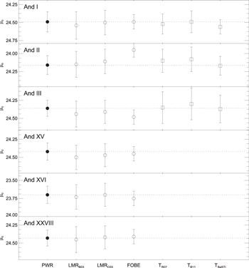
Figure 10. Summary of our derived distances. Circles report values based on RRL stars, while squares are based on the TRGB (provided only for the most massive galaxies, for which the TRGB could be reliably estimated). The filled circles and the dotted lines show the measurements based on the PWR, which are the final adopted distances. Open symbols show values obtained with the other methods for comparison.
Download figure:
Standard image High-resolution image6.7. Comparison with Previous Works
Figure 11 displays a comparison with distance estimates available in the literature and derived with different techniques: RRL stars (open triangles: Pritzl et al. 2004, 2005), the HB luminosity (open diamonds: Da Costa et al. 1996, 2000; Slater et al. 2015), and the TRGB (open stars: Mould & Kristian 1990; Koenig et al. 1993; McConnachie et al. 2004, 2005; Letarte et al. 2009; Conn et al. 2012). This figure shows an overall good agreement with our estimates within the uncertainties. We note that the TRGB tends to provide closer distances than the RRL and the HB luminosity, although it is still compatible within 1.5σ. Several discrepant cases (And XV and XVI from Conn et al. 2012) can be ascribed to the sparsely populated bright portion of the RGB in these galaxies.
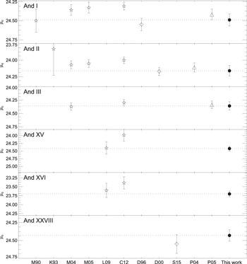
Figure 11. Comparison of our adopted distance moduli (based on the PWR, filled circles and dotted lines) with the literature values (open symbols). In particular, we report values based on the TRGB (stars: Mould & Kristian 1990; Koenig et al. 1993; McConnachie et al. 2004, 2005; Letarte et al. 2009; Conn et al. 2012), HB luminosity (diamond: Da Costa et al. 1996, 2000; Slater et al. 2015), and RRL stars (triangles: Pritzl et al. 2004, 2005).
Download figure:
Standard image High-resolution image7. Other Variables
7.1. Anomalous Cepheid Stars
AC stars are variable stars in the core He-burning evolutionary phase at a luminosity that is higher than that of RRL stars. Their periods range from ∼0.5 to ∼2.0 days and their masses are thought to be higher than 1  . In order to have ACs with such masses, two different channels are likely (Bono et al. 1997; Gallart et al. 2004; Cassisi & Salaris 2013). They can be the progeny of coalesced binary stars, that is, evolved blue straggler stars (BSS) tracing the old population (Renzini et al. 1977; Hirshfeld 1980; Sills et al. 2009). Alternatively, they can be an evolutionary stage of single stars with mass between ∼1.2 and ∼2.2
  and age between 1 and 6 Gyr (Demarque & Hirshfeld 1975; Norris & Zinn 1975; Castellani & Degl'Innocenti 1995; Caputo et al. 1999; Dolphin et al. 2002; Fiorentino et al. 2006). In both scenarios, they trace the existence of a metal-poor (Z < 0.0006) stellar population, thus providing sound constraints to the metal enrichment of the galaxy.
Typically, purely old (age  Gyr) nearby LG dwarf galaxies host a few ACs. However, they are very rare in GCs; so far, only one candidate has been confirmed in the metal-poor ([Fe/H] ∼ −2 dex) cluster NGC 5466 (Zinn & Dahn 1976), and a few others have been suggested (Corwin et al. 1999; Arellano Ferro et al. 2008; Kuehn et al. 2011; Walker et al. 2017). On the other hand, large samples of ACs have been collected in the LMC (141) and in the SMC (109) in the framework of the OGLE-IV project (Soszyński et al. 2015). In this context, it is worth mentioning that the work of Mateo et al. (1995)—updated by Fiorentino & Monelli (2012), who collected data from nearby dwarf galaxies with an established SFH and in which ACs have been found (see their Figure 7)—noted a correlation between the frequency of ACs and the total luminosity of the host galaxy; the frequency of ACs decreases for increasing luminosity of the host galaxy. Another parameter that seems to impact the ACs frequency is the SFH of the host system, with primarily old systems, or fast galaxies (as defined by Gallart et al. 2015) having a lower specific frequency of ACs than systems containing many intermediate-age and young populations (slow galaxies).
Figure 1 shows the presence of a few variable stars located 1 to 2 mag above the HB. Given their pulsation properties, their position in the period-Wesenheit diagram (see e.g., Figure 1 in Fiorentino & Monelli 2012), and the shape of their LCs, we classify them as ACs. In particular, a total of 15 ACs have been detected in the ACS field of And II, III, XV, and XXVIII. No ACs have been detected in And I, in agreement with Pritzl et al. (2005), or in And XVI. The lack of ACs in And I can be a hint of the fast chemical enrichment of this galaxy. This is supported by the high metallicity of this galaxy when compared with the remaining ISLAndS galaxies. On the other hand, And XVI has the proper mean low metallicity, but its low total mass is the most probable cause for the lack of ACs. Interestingly, And XVI shows active star formation until about 6 Gyr ago, thus not extended enough to produce ACs through the single-star channel.
As none of the four ISLAndS galaxies where ACs have been detected shows evidence of star formation younger than 2 Gyr (Skillman et al. 2017), it is unlikely that ACs come from the evolution of a young metal-poor star. The sequence of blue objects between the oldest MSTO and the HB are most likely BSS descending from primordial binary stars of the old population, in agreement with the SFHs obtained by Skillman et al. (2017). Therefore we assume that the AC we detected here are the progeny of coalesced binary stars (evolved BSS), thus tracing the old population (Renzini et al. 1977; Hirshfeld 1980; Sills et al. 2009).
From our sample, only four ACs were previously known28 : AndII-V083 (V14 by Pritzl et al. 2004), AndIII-V073, AndIII-V075, and AndIII-V105 (V01, V07, and V06 by Pritzl et al. 2005). The LCs of all the detected ACs are shown in Figure 12. The different shapes are an indication of different pulsational modes. However, the classification of the pulsation mode of ACs is not trivial and cannot be easily determined from the morphology of the LCs alone (Marconi et al. 2004).
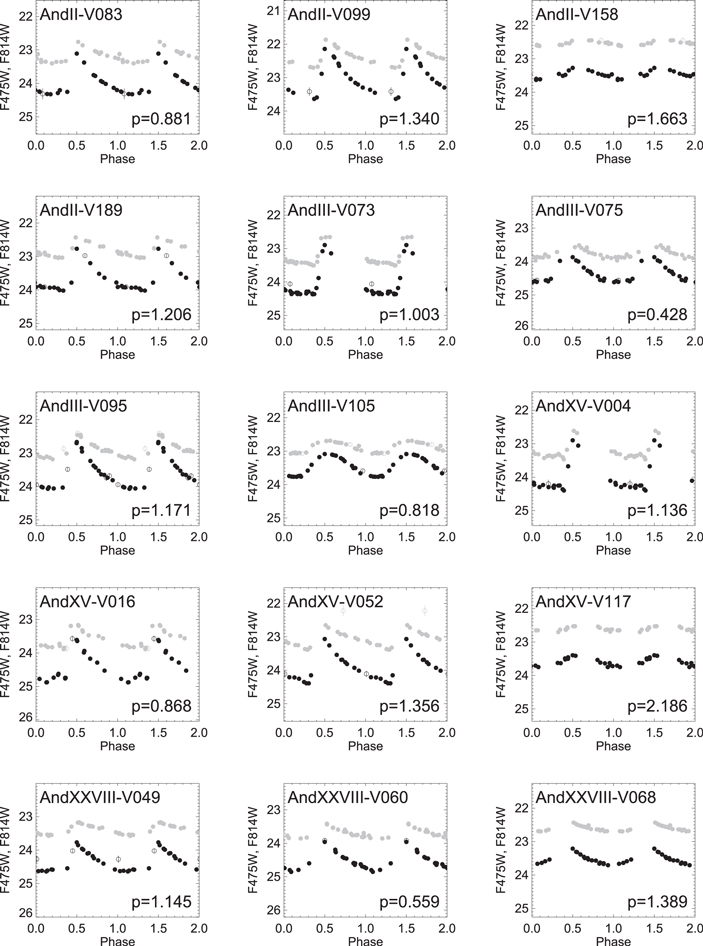
Figure 12. Light curves of member AC stars for four of the six ISLAndS galaxies in the  (black) and
  (gray) bands. Periods (in days) are given in the lower right corner, while the name of the variable is displayed at the top of each panel. Open symbols show the data for which the uncertainties are larger than 3σ above the mean error of a given star; these data were not used in period and mean-magnitude calculations.
Download figure:
Standard image High-resolution imageFigure 13 shows the period-Wesenheit plane for the reddening-free index W( –I)—which reduces the scatter due to the interstellar reddening and the intrinsic width of the IS—for the ACs of the LMC (open symbols) published by the OGLE collaboration (Soszyński et al. 2015). This plot shows a clear separation between fundamental (F, black dots) and first-overtone (FO, open circles) pulsators for ACs. Therefore, ACs are defined by different PL relations, and fundamental and first-overtone pulsation can also be distinguished in this way. We therefore overplot the 15 ACs found in this work with the aim of checking their nature and identifying their pulsation modes. The four ACs found in And II are represented by red circles, the four in And III by green squares, the four in And XV by orange diamonds, and the three in And XXVIII by blue triangles. First, Figure 13 supports their classification as ACs. We note that only one star (And XXVIII-V068) is somewhat distant from the bulk of the F mode ACs of the LMC. From an inspection of the LC of this star (see Figure 12), the lack of phase points close to the maximum light is evident. Therefore, the measurement of the mean magnitude of this star may be biased to brighter magnitude, as the fit with templates tends to overestimate the amplitude. Figure 13 indicates that the majority of the ACs (12) are pulsating in the F mode, and only three of them (And III-V075, And III-V105, and And XXVIII-V060) are FO pulsators.
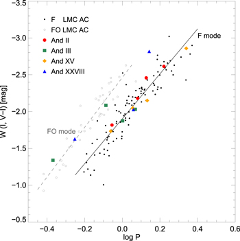
Figure 13. Period-Wesenheit diagram for ACs. Black dots (F pulsators) and gray circles (FO pulsators) represent the ACs of the LMC from the OGLE-IV release (Soszyński et al. 2015). ACs discovered in our galaxies are represented by red circles (And II), green squares (And III), orange diamonds (And XV), and blue triangles (And XXVIII). The solid and dashed lines are the empirical period–luminosity relations obtained by Soszyński et al. (2015) for ACs in the LMC for the F and FO mode, respectively.
Download figure:
Standard image High-resolution image7.2. Eclipsing Binary Candidates
For the sake of completeness, we report the detection of three EBs, one in And I and two in And II. Figure 14 shows their LCs, which in all cases show a minimum. For the three candidates, the minimum occurs at the same phase in the two bands. This feature, together with the flat bright part of the LCs, the periods, and their position in the CMD, supports the classification as EBs.
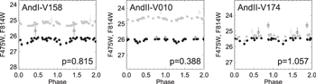
Figure 14. Light curves of the three EB candidates detected in the field of And I and And II in the  (black) and
  (gray) bands. Periods (in days) are given in the lower right corner, while the name of the variable is displayed at the top of each panel. Open symbols show the data for which the uncertainties are larger than 3σ above the mean error of a given star; these data were not used in period and mean-magnitude calculations.
Download figure:
Standard image High-resolution imageThe fact that only such a small number of candidate EBs was detected is due to both the relatively small number of points per LC taken, the non-optimal time sampling for this type of variable, and the limited region of the CMD that was searched for variables.
8. Summary and Final Remarks
In this paper we have analyzed multi-epoch HST data for six dSphs satellites of M31 in order to study their population of variable stars. The main findings of the current study are listed below.
- 1.We have detected 895 variable stars in And I, II, III, XV, XVI, and XXVIII: 678 of them are new discoveries. In particular, we classified 870 RRL stars, 15 ACs, 3 EB, and 7 field variable stars (5 of them probably belonging to the GSS of M31). Interestingly, no ACs were found in And I, although it is the second most massive dwarf in our sample; we interpret this as a hint of the fast chemical enrichment of this galaxy.
- 2.Pulsational properties (period, amplitude, and mean magnitude) were derived for all detected variables. Moreover, we provide all the LCs and time-series photometry.
- 3.Using the properties of RRL stars, we derived new homogeneous distances to the six galaxies using three different methods: the PWR, the metallicity–luminosity relation, and the first-overtone blue-edge method. A fourth independent estimate was derived using the tip of the RGB for the three most populated systems. We find a satisfactory agreement both between different methods and with most of the estimates available in the literature. It is worth noting that the values obtained using the RRL stars are more accurate and precise. For these reasons, we adopted as final distance moduli those that were obtained through the PWR, which are the most precise values and based on the most recently updated relation for RRLs to date.
- 4.We have shown that similar to MW satellites, the mean period of RRab variables of the six ISLAndS is close to 0.6 day, a value that is typical of Oo-intermediate objects. On the other hand, the distribution of RRL stars in the Bailey diagram is such that the majority of stars (∼80%) are distributed close to the locus of Oo-I type. And XXVIII appears to be a peculiar object, both because the RRab stars do not follow any Oosterhoff relation in particular, and because the fraction of RRc-type stars is the largest among nearby galaxies.
- 5.In spite of the slight difference in the HB morphology parameter (RHB), when we restrict the comparison between M31 and MW systems to the properties of RRL stars alone, we do not find significant differences between the two groups of galaxies. In particular, based on a sample of 16 satellites of M31 and 15 of MW, we find a similar trend between the mean period and the mean metallicity. This suggests overall similar characteristics of the oldest (>10 Gyr) population in the two systems, in agreement with what is discussed by Monelli et al. (2017) using the global period distributions of thousands of RRL stars belonging to faint and bright satellites of M31 and the MW.
To date, none of the known LG dwarf galaxies has a complete census of their entire population of variable stars. However, we are at the dawn of a new era for variability studies. Current and future surveys are about to bring an unprecedented amount of information on the variable stars populating the surroundings of the MW and of the LG. Gaia will enable the discovery of thousands of new RRL stars ( mag) in the MW Halo (Clementini et al. 2016, DR1), and will in particular help us to complete the census of RRL stars in some MW satellites (Antoja et al. 2015). Additionally, the LSST will produce a flood of data that will enable the discovery of a highly complete sample of RRL stars out to hundreds of kpc.
Finally, regarding RRL stars in the M31 satellites, the large number of dwarf galaxies discovered in this system during the last few years remain largely unexplored. The advent of the wide-field imaging capability of telescopes, such as WFIRST (with a field of view roughly 100 times greater than that of HST), could substantially accelerate these studies and offer us the possibility to understand the similarities and differences between the two systems of the LG: MW and M31 satellites.
The authors thank the anonymous referee for the useful comments that helped to improve the manuscript. This research made extensive use of NASA's Astrophysics Data System Bibliographic Services and the NASA/IPAC Extragalactic Database (NED), which is operated by the Jet Propulsion Laboratory, California Institute of Technology, under contract with the National Aeronautics and Space Administration. Support for this work was provided by NASA through grants GO-13028 and GO-13749 from the Space Telescope Science Institute, which is operated by AURA, Inc., under NASA contract NAS5-26555. This work has also been supported by the Spanish Ministry of Economy and Competitiveness (MINECO) under the grant (project reference AYA2014-56795-P). EJB acknowledges support from the CNES postdoctoral fellowship program. G.F. has been supported by the Futuro in Ricerca 2013 (grant RBFR13J716). Support for D.R.W. is provided by NASA through Hubble Fellowship grants HST-HF-51331.01 awarded by the Space Telescope Science Institute.
Facility: HST - Hubble Space Telescope satellite(ACS, WFC3).
Software: IDL, DAOPHOT/ALLFRAME.
Appendix A: Observing Logs for ISLAnds Galaxies
This work is based on observations obtained with the ACS and WFC3 on board the HST. These data were collected in different runs for each galaxy over about 2 and 5.3 consecutive days between 2013 October 4 to 2015 September 6 as part of a large HST proposal (GO-13028 and GO-13749, P.I.: E. Skillman). The observing sequence consisted of alternating ∼1100 s exposures in F475W and F814W for an optimal sampling of the LCs. The complete observing logs for And I, II, III, XV, XVI, and XXVIII are given in Table 9. Individual galaxy tables are available in the online version of this article. These tables collect the name of the image (column 1) as it appears in the HST archive (http://archive.stsci.edu/), the date (column 2), and the UT start of each exposure (column 3), the filter used (column 4), and the exposure time (column 5).
Table 9. Observing Log for the ISLAndS Galaxies
| Image Name | Date | UT Start | Filter | Exp. Time |
|---|---|---|---|---|
| (YYYY-MM-DD) | (hh:mm:ss) | name | (s) | |
| And I | ||||
| ACS (R.A. = 00:45:42.8, decl. = +38:02:22.8) | ||||
| jcnb01lyq_flc.fits | 2015 Sep 01 | 09:56:05 | F475W | 1264 |
| jcnb01m1q_flc.fits | 2015 Sep 01 | 10:20:06 | F814W | 1002 |
| WFC3 (R.A. = 00:45:14.2, decl. = +38:00:03.0) | ||||
| icnb01lzq_flc.fits | 2015 Sep 01 | 09:55:10 | F475W | 1308 |
| icnb01m0q_flc.fits | 2015 Sep 01 | 10:19:26 | F814W | 1046 |
| And II | ||||
| ACS (R.A. = 01:16:23.8, decl. = +33:26:05.5) | ||||
| jc1d01wfq_flc.fits | 2013 Oct 04 | 03:50:09 | F475W | 1280 |
| jc1d01whq_flc.fits | 2013 Oct 04 | 04:14:26 | F814W | 987 |
| WFC3 (R.A. = 01:16:04.4, decl. = +33:21:31.7) | ||||
| ic1d01wgq_flc.fits | 2013 Oct 04 | 03:49:14 | F475W | 1350 |
| ic1d01wiq_flc.fits | 2013 Oct 04 | 04:14:12 | F814W | 1122 |
| And III | ||||
| ACS (R.A. = 00:35:30.7, decl. = +36:30:14.2) | ||||
| jcnb12c4q_flc.fits | 2014 Nov 24 | 05:33:55 | F475W | 1264 |
| jcnb12c7q_flc.fits | 2014 Nov 24 | 05:57:56 | F814W | 1002 |
| WFC3 (R.A. = 00:35:51.5, decl. = +36:25:48.5) | ||||
| icnb12c5q_flc.fits | 2014 Nov 24 | 05:33:00 | F475W | 1308 |
| icnb12c6q_flc.fits | 2014 Nov 24 | 05:57:16 | F814W | 1046 |
| And XV | ||||
| ACS (R.A. = 01:14:18.7, decl. = +38:07:03.0) | ||||
| jcnb23w3q_flc.fits | 2014 Sep 17 | 11:23:38 | F475W | 1264 |
| jcnb23w6q_flc.fits | 2014 Sep 17 | 11:47:39 | F814W | 1002 |
| WFC3 (R.A. = 01:13:50.3, decl. = +38:04:37.3) | ||||
| icnb23w4q_flc.fits | 2014 Sep 17 | 11:22:43 | F475W | 1308 |
| icnb23w5q_flc.fits | 2014 Sep 17 | 11:46:59 | F814W | 1046 |
| And XVI | ||||
| ACS (R.A. = 00:59:32.3, decl. = +32:23:38.9) | ||||
| jc1d09upq_1.fits | 2013 Nov 20 | 12:46:13 | F475W | 1280 |
| jc1d09urq_1.fits | 2013 Nov 20 | 13:10:30 | F814W | 987 |
| WFC3 (R.A. = 00:59:48.6, decl. = +32:18:37.2) | ||||
| ic1d09uqq_flc.fits | 2013 Nov 20 | 12:45:18 | F475W | 1350 |
| ic1d09usq_flc.fits | 2013 Nov 20 | 13:10:16 | F814W | 1122 |
| And XXVIII | ||||
| ACS (R.A. = 22:32:41.2, decl. = +31:12:58.2) | ||||
| jcnb31psq_flc.fits | 2015 Jan 20 | 23:57:41 | F475W | 1264 |
| jcnb31pvq_flc.fits | 2015 Jan 21 | 00:21:42 | F814W | 1002 |
| WFC3 (R.A. = 22:33:09.6, decl. = +31:13:31.0) | ||||
| icnb31ptq_flc.fits | 2015 Jan 20 | 23:56:46 | F475W | 1308 |
| icnb31puq_flc.fits | 2015 Jan 21 | 00:21:02 | F814W | 1046 |
Only a portion of this table is shown here to demonstrate its form and content. A machine-readable version of the full table is available.
Download table as: DataTypeset image
Appendix B: Time Series of Variable Stars in ISLAndS Galaxies
The individual  and
and  measurements for all of the variables found in each galaxy of this work are listed in Table 10. Individual galaxy tables are available in the online version of this article.
Table 10. Photometry of the Variable Stars in the ISLAndS Galaxies
| Star | MHJD* |

|

|
MHJDa |

|

|
|---|---|---|---|---|---|---|
| And I | ||||||
| AndI-V001 | 57266.425781 | 25.254 | 0.089 | 57266.441406 | 24.713 | 0.090 |
| AndI-V001 | 57266.500000 | 25.523 | 0.056 | 57266.484375 | 24.417 | 0.119 |
| AndI-V001 | 57266.691406 | 25.801 | 0.041 | 57266.707031 | 24.953 | 0.067 |
| AndI-V001 | 57266.765625 | 25.917 | 0.064 | 57266.750000 | 25.028 | 0.093 |
| AndI-V001 | 57267.417969 | 25.175 | 0.036 | 57267.433594 | 24.364 | 0.043 |
| AndI-V001 | 57267.496094 | 25.118 | 0.036 | 57267.480469 | 24.549 | 0.064 |
| AndI-V001 | 57267.683594 | 25.733 | 0.062 | 57267.699219 | 24.876 | 0.054 |
| AndI-V001 | 57267.761719 | 25.863 | 0.052 | 57267.746094 | 25.007 | 0.127 |
| And II | ||||||
| AndII-V001 | 56569.171875 | 24.838 | 0.031 | 56569.187500 | 24.319 | 0.047 |
| AndII-V001 | 56569.253906 | 24.822 | 0.051 | 56569.234375 | 24.196 | 0.047 |
| AndII-V001 | 56569.437500 | 25.382 | 0.041 | 56569.453125 | 24.654 | 0.061 |
| AndII-V001 | 56569.519531 | 24.785 | 0.069 | 56569.500000 | 24.326 | 0.059 |
| AndII-V001 | 56570.101562 | 25.326 | 0.042 | 56570.117188 | 24.509 | 0.058 |
| AndII-V001 | 56570.183594 | 24.775 | 0.048 | 56570.164062 | 24.268 | 0.047 |
| AndII-V001 | 56570.500000 | 24.833 | 0.036 | 56570.515625 | 24.399 | 0.051 |
| And III | ||||||
| AndIII-V001 | 56985.244721 | 25.181 | 0.034 | 56985.259883 | 24.593 | 0.036 |
| AndIII-V001 | 56985.317071 | 25.254 | 0.021 | 56985.300786 | 24.459 | 0.035 |
| AndIII-V001 | 56985.443750 | 25.538 | 0.047 | 56985.458912 | 24.765 | 0.038 |
| AndIII-V001 | 56985.516204 | 25.525 | 0.048 | 56985.499919 | 24.701 | 0.062 |
| AndIII-V001 | 56985.642767 | 25.035 | 0.040 | 56985.657929 | 24.488 | 0.048 |
| AndIII-V001 | 56985.721413 | 24.881 | 0.149 | 56985.705128 | 24.540 | 0.038 |
| AndIII-V001 | 56986.239807 | 25.663 | 0.046 | 56986.254969 | 24.688 | 0.059 |
| And XV | ||||||
| AndXV-V001 | 56917.486432 | 24.553 | 0.033 | 56917.501594 | 24.281 | 0.036 |
| AndXV-V001 | 56917.564258 | 25.095 | 0.039 | 56917.547973 | 24.378 | 0.030 |
| AndXV-V001 | 56918.682087 | 25.631 | 0.055 | 56918.697250 | 24.707 | 0.048 |
| AndXV-V001 | 56918.758837 | 25.772 | 0.053 | 56918.742552 | 24.872 | 0.067 |
| AndXV-V001 | 56918.881259 | 25.826 | 0.056 | 56918.896422 | 24.939 | 0.064 |
| AndXV-V001 | 56918.957951 | 25.254 | 0.098 | 56918.941666 | 24.810 | 0.057 |
| AndXV-V001 | 56919.476714 | 24.797 | 0.034 | 56919.491877 | 24.240 | 0.038 |
| And XVI | ||||||
| AndXVI-V001 | 56616.545139 | 25.496 | 0.025 | 56616.560301 | 24.366 | 0.153 |
| AndXVI-V001 | 56616.621076 | 25.675 | 0.034 | 56616.604792 | 24.668 | 0.042 |
| AndXVI-V001 | 56617.010037 | 25.030 | 0.024 | 56617.025199 | 24.462 | 0.056 |
| AndXVI-V001 | 56617.085986 | 25.392 | 0.022 | 56617.069701 | 24.566 | 0.029 |
| AndXVI-V001 | 56617.408499 | 25.885 | 0.050 | 56617.423673 | 24.846 | 0.054 |
| AndXVI-V001 | 56617.484483 | 25.923 | 0.063 | 56617.468199 | 24.823 | 0.057 |
| AndXVI-V001 | 56617.674172 | 25.619 | 0.043 | 56617.689334 | 24.660 | 0.054 |
| And XXVIII | ||||||
| AndXXVIII-V001 | 57043.010749 | 25.951 | 0.110 | 57043.025911 | 24.779 | 0.060 |
| AndXXVIII-V001 | 57043.082797 | 25.813 | 0.054 | 57043.066513 | 24.845 | 0.031 |
| AndXXVIII-V001 | 57043.209741 | 25.053 | 0.062 | 57043.224903 | 24.318 | 0.052 |
| AndXXVIII-V001 | 57043.281893 | 24.992 | 0.038 | 57043.265608 | 24.327 | 0.039 |
| AndXXVIII-V001 | 57044.204663 | 25.908 | 0.053 | 57044.219825 | 24.515 | 0.075 |
| AndXXVIII-V001 | 57044.277290 | 25.903 | 0.043 | 57044.261005 | 24.683 | 0.175 |
| AndXXVIII-V001 | 57044.337289 | 25.878 | 0.077 | 57044.352451 | 24.875 | 0.046 |
Note.
aModified Heliocentric Julian Date of mid-exposure: HJD—2,400,000.Only a portion of this table is shown here to demonstrate its form and content. A machine-readable version of the full table is available.
Download table as: DataTypeset image
Appendix C: Comparison with the Literature
Figure 15 compares the periods of variable stars in common between our work and the published period for the three galaxies that have been studied in the literature (And I, And II, and And III; Pritzl et al. 2004, 2005), according to the labeled symbols. Pritzl's data for each galaxy consist of two data sets separated by 4–5 days. In each data set, they first started observing all the  and then all the
  images. The cadence of the data depends on the individual case. For And I, the strategy was
  (
( ) and
) and  (
( ) in the first (second) set, with one image per orbit. For And II, the data were collected as
  (
( ) and
) and  (
( ) in the first (second) set, with two images per orbit. For And III, the strategy was similar to that for And II, but collecting
  and
and  in each data set.
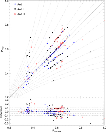
Figure 15. Current period vs. the period (top) and period difference (bottom) found by Pritzl et al. (2004, 2005) for the 94, 69, and 54 stars matched in And I (black circles), And II (blue plusses), and And III (red open squares), respectively. The dotted curves in the top panel are the aliasing lines (see text). We have taken the HST orbital period (96 minutes) as fsampling and ![$| N| =[1,3,6,9,15,18]$](https://content.cld.iop.org/journals/0004-637X/850/2/137/revision1/apjaa9381ieqn290.gif) to obtain these curves (aliasing lines). Note that the outliers follow the aliasing lines in most cases. This indicates the high probability that the offsets are due to aliasing.
to obtain these curves (aliasing lines). Note that the outliers follow the aliasing lines in most cases. This indicates the high probability that the offsets are due to aliasing.
Download figure:
Standard image High-resolution imageA total of 94, 69, and 54 stars (out of 100, 73, and 56 in their catalogs) were recovered for And I, And II, and And III, respectively. The cross-identifications made between our catalogs and Pritzl's are shown in Table 11. Individual galaxy tables are available in the online version of this article. The small fraction of stars that were not recovered either appear as non-variable in our data or fall in the ACS gap (see the column "Notes" of Table 11). We note that the matching was complicated by the fact that the coordinates listed in the Pritzl catalogs were significantly offset, with different offsets for each WFPC2 chip, in particular in the case of And III.
Table 11. Cross-identification with the Pritzl et al. Catalogs of Variable Stars in And I, And II, and And III
| IDPritzl | PeriodPritzl | ID
|
Period
|
Notes |
|---|---|---|---|---|
| And I | ||||
| V1 | 1.630 | ⋯ | ⋯ | near to the BSS region; affected by |
| near saturated field star; not variable in our data | ||||
| V2 | 0.348 | And I-V185 | 0.349 | |
| V3 | 0.412 | And I-V182 | 0.386 | |
| V4 | 9.999 | And I-V172 | 0.607 | |
| V5 | 0.654 | And I-V154 | 0.746 | |
| V6 | 0.430 | And I-V186 | 0.429 | |
| ⋯ | ⋯ | ⋯ | ⋯ | ⋯ |
| V44 | 0.748 | ⋯ | ⋯ | minor variation in F814; not variable in our data |
| V45 | 0.772 | ⋯ | ⋯ | not variable in our data |
| ⋯ | ⋯ | ⋯ | ⋯ | ⋯ |
| V89 | 0.523 | ⋯ | ⋯ | in ACS gap |
| ⋯ | ⋯ | ⋯ | ⋯ | ⋯ |
| V98 | 0.625 | ⋯ | ⋯ | in ACS gap |
| V99 | 0.716 | AndI-V237 | 0.630 | |
| V100 | 0.782 | ⋯ | ⋯ | not variable in our data |
| And II | ||||
| V01 | 0.407 | AndII-V080 | 0.370 | |
| V02 | 0.546 | AndII-V071 | 0.543 | |
| V03 | 0.520 | AndII-V098 | 0.516 | |
| V04 | 0.540 | AndII-V064 | 0.692 | |
| V05 | 0.583 | AndII-V081 | 0.580 | |
| ⋯ | ⋯ | ⋯ | ⋯ | ⋯ |
| V16 | 0.346 | ⋯ | ⋯ | not variable in our data |
| ⋯ | ⋯ | ⋯ | ⋯ | ⋯ |
| V37 | 0.751 | ⋯ | ⋯ | not variable in our data |
| ⋯ | ⋯ | ⋯ | ⋯ | ⋯ |
| V43 | 0.490 | ⋯ | ⋯ | in ACS gap |
| ⋯ | ⋯ | ⋯ | ⋯ | ⋯ |
| V70 | 0.707 | ⋯ | ⋯ | not variable in our data |
| V71 | 0.474 | AndII-V153 | 0.580 | |
| V72 | 0.469 | AndII-V087 | 0.592 | |
| V73 | 0.698 | AndII-V118 | 0.538 | |
| And III | ||||
| V01 | 0.834 | AndIII-V073 | 1.003 | |
| V02 | 0.590 | AndIII-V069 | 0.591 | |
| V03 | 0.773 | ⋯ | ⋯ | in ACS gap |
| V04 | 0.629 | AndIII-V065 | 0.559 | |
| V05 | 0.650 | AndIII-V067 | 0.632 | |
| V06 | 0.678 | AndIII-V105 | 0.818 | |
| V07 | 0.480 | AndIII-V075 | 0.428 | |
| V08 | 1.510 | ⋯ | ⋯ | not variable in our data |
| ... | ... | ... | ... | ... |
| V53 | 0.534 | AndIII-V039 | 0.533 | |
| V54 | 0.623 | AndIII-V041 | 0.625 | |
| V55 | 0.599 | AndIII-V031 | 0.596 | |
| V56 | 0.496 | AndIII-V046 | 0.640 | |
Only a portion of this table is shown here to demonstrate its form and content. A machine-readable version of the full table is available.
Download table as: DataTypeset image
The comparison discloses a general good agreement (53% of the stars within a difference of 0.05 days and 80% within 0.1 days), although with a few outliers for which the period is significantly discrepant (20% have a difference larger than 0.1 day). However, this effect can be easily explained by taking into account that HST observations may suffer from a strong aliasing introduced by the orbital time. By having more epochs and scheduling them to avoid redundant periods, our program strongly suppressed the effects of aliasing.
The aliasing effect is a very common error in signal treatment because it happens whenever the original periodic signal (in our case, the LC of the variable stars) is reconstructed using a discrete sampling. When a periodic signal of frequency ftrue is sampled with a frequency fsampling, the resulting number of cycles per sample is  (normalized frequency), and the samples are indistinguishable from those of another sinusoid (or periodic signal), called an alias, whose normalized frequency differs from
  by an integer (see e.g., VanderPlas 2017). Then, we can express the aliases of frequency as
  , where N is an integer. In this case, the calculation of the period can be affected by the HST orbital cadence of 96 minutes.
The curves overplotted on Figure 15 represent how the true period is affected by a cadence of 96 minutes. Interestingly, most if not all the discrepant points are explained by this aliasing effect. Taking into account the limited number of phase points in previous studies and the optimized strategy of our observations, we suggest that this has resulted in more precise period determinations. Nevertheless, this comparison also supports the quality of the previous analyses, given the observational material available.
Appendix D: Pulsation Properties of Variable Stars in ISLAndS Galaxies
The properties of the variable stars found in this work for And I, II, III, XV, XVI, and XXVIII are detailed in Table 12. Individual galaxy tables are available in the online version of this article. The first columns give the identification number, and the next two list the equatorial coordinates (J2000.0). Column 4 give the period of the variable in days, while columns 5 to 14 list the intensity-averaged magnitudes and amplitude in the filters  , and I, respectively. The last column displays the variable type.
Table 12. Pulsation Parameters of the Variable Stars in the ISLAndS Galaxies
| ID | R.A. | Decl. | Period |

|

|

|

|

|
AB |

|
AV |

|
AI | Type |
|---|---|---|---|---|---|---|---|---|---|---|---|---|---|---|
| Name | (J2000) | (J2000) | (Current) | |||||||||||
| And I | ||||||||||||||
| AndI-V001 | 0:45:09.233 | +37:58:47.19 | 0.569 | 25.532 | 1.038 | 24.692 | 0.574 | 25.657 | 1.137 | 25.266 | 0.915 | 24.677 | 0.580 | RRab |
| AndI-V002 | 0:45:09.646 | +37:59:48.86 | 0.567 | 25.505 | 0.590 | 24.737 | 0.358 | 25.613 | 0.669 | 25.251 | 0.436 | 24.719 | 0.360 | RRab |
| AndI-V003 | 0:45:09.819 | +37:59:32.31 | 0.296 | 25.329 | 0.336 | 24.831 | 0.091 | 25.398 | 0.392 | 25.159 | 0.207 | 24.819 | 0.097 | RRc |
| And II | ||||||||||||||
| AndII-V001 | 1:15:56.325 | +33:21:19.95 | 0.332 | 25.061 | 0.686 | 24.441 | 0.336 | 25.149 | 0.747 | 24.848 | 0.563 | 24.425 | 0.330 | RRc |
| AndII-V002 | 1:15:57.224 | +33:21:32.52 | 0.601 | 25.064 | 1.016 | 24.272 | 0.362 | 25.310 | 0.948 | 24.785 | 0.685 | 24.239 | 0.325 | RRab |
| AndII-V003 | 1:15:58.620 | +33:21:29.91 | 0.625 | 25.115 | 0.766 | 24.243 | 0.375 | 25.257 | 0.886 | 24.811 | 0.613 | 24.231 | 0.383 | RRab |
| And III | ||||||||||||||
| AndIII-V001 | 0:35:22.101 | +36:29:14.19 | 0.400 | 25.357 | 0.568 | 24.585 | 0.299 | 25.486 | 0.644 | 25.079 | 0.481 | 24.570 | 0.303 | RRd |
| AndIII-V002 | 0:35:22.192 | +36:29:30.74 | 0.645 | 25.410 | 0.710 | 24.493 | 0.467 | 25.551 | 0.781 | 25.107 | 0.591 | 24.490 | 0.445 | RRab |
| AndIII-V003 | 0:35:22.642 | +36:31:02.97 | 0.655 | 25.325 | 0.973 | 24.477 | 0.506 | 25.461 | 1.071 | 25.030 | 0.730 | 24.464 | 0.510 | RRab |
| And XV | ||||||||||||||
| AndXV-V001 | 1:14:10.037 | +38:06:34.23 | 0.503 | 25.366 | 1.443 | 24.657 | 0.761 | 25.469 | 1.552 | 25.128 | 1.215 | 24.643 | 0.760 | RRab |
| AndXV-V002 | 1:14:10.426 | +38:06:37.79 | 0.618 | 25.364 | 0.861 | 24.523 | 0.458 | 25.494 | 0.948 | 25.071 | 0.707 | 24.508 | 0.465 | RRab |
| AndXV-V003 | 1:14:10.438 | +38:06:38.32 | 0.587 | 25.312 | 1.015 | 24.541 | 0.633 | 25.429 | 1.089 | 25.047 | 0.876 | 24.524 | 0.640 | RRab |
| And XVI | ||||||||||||||
| AndXVI-V001 | 0:59:24.386 | +32:22:33.16 | 0.622 | 25.459 | 1.142 | 24.642 | 0.555 | 25.584 | 1.281 | 25.173 | 0.912 | 24.627 | 0.571 | M31 RRL |
| AndXVI-V002 | 0:59:25.335 | +32:22:16.10 | 0.358 | 24.563 | 0.624 | 23.877 | 0.402 | 24.671 | 0.692 | 24.306 | 0.484 | 23.857 | 0.394 | RRc |
| AndXVI-V003 | 0:59:27.972 | +32:22:57.58 | 0.389 | 24.560 | 0.552 | 23.791 | 0.374 | 24.667 | 0.612 | 24.313 | 0.445 | 23.774 | 0.375 | RRc |
| And XXVIII | ||||||||||||||
| AndXXVIII-V001 | 22:32:32.098 | +31:13:11.52 | 0.642 | 25.549 | 1.142 | 24.648 | 0.601 | 25.694 | 1.259 | 25.229 | 0.960 | 24.639 | 0.620 | RRab |
| AndXXVIII-V002 | 22:32:33.432 | +31:13:07.56 | 0.608 | 25.392 | 0.697 | 24.659 | 0.228 | 25.508 | 0.590 | 25.141 | 0.392 | 24.615 | 0.203 | RRL? |
| AndXXVIII-V003 | 22:32:35.539 | +31:12:15.41 | 0.407 | 25.414 | 0.460 | 24.603 | 0.217 | 25.536 | 0.517 | 25.131 | 0.366 | 24.587 | 0.222 | RRc |
Note. And I: Stars from "AndI-V001" to "AndI-V0038" were detected in the WFC3 field, while stars from "AndI-V039" to "AndI-V314" were detected in the ACS field. And II: Stars from "AndII-V001" to "AndII-V0035" were detected in the WFC3 field, while stars from "AndII-V036" to "AndII-V260" were detected in the ACS field. And III: Stars from "AndIII-V001" to "AndIII-V114" were detected in the ACS field, while stars from "AndIII-V115" to "AndIII-V118" were detected in the WFC3 field. And XV: All stars were detected in the ACS field. And XVI: All stars were detected in the ACS field. And XXVIII: All stars were detected in the ACS field.
Only a portion of this table is shown here to demonstrate its form and content. A machine-readable version of the full table is available.
Download table as: DataTypeset image
Footnotes
- ∗
Based on observations made with the NASA/ESA Hubble Space Telescope, obtained at the Space Telescope Science Institute, which is operated by the Association of Universities for Research in Astronomy, Inc., under NASA contract NAS 5-26555. These observations are associated with programs
 and 13739.
 - 16
Initial Star formation and Lifetimes of Andromeda Satellites.
- 17
Other types of variable stars, such as long-period RGB/AGB stars or very short-period stars such as δ-Scuti cannot be detected or properly characterized with the current data set, so we focused on the core helium-burning stars alone.
- 18
Excluding the RRL star AndXVI-V001 (V0 in Monelli et al. 2016) as it is a candidate M31 halo field star not belonging to And XVI.
- 19
- 20
The other two most likely belong to the M31 GSS, see Section 4.2 for further details.
- 21
RHB = (B − R)/(B+V+R), where B and R are the numbers of HB stars bluer and redder than the IS, respectively, and V is the number of RRL stars (Lee 1990).
- 22
In the case of And II, Kalirai et al. (2010) estimate both a photometric and a spectroscopic metallicity, concluding that with the data at hand, the former is less dependent on the low S/N of the measurements.
- 23
- 24
- 25
And XVI only has five RRc stars.
- 26
We note that the zero-point of this theoretical calibration has been corrected in order to account for the impact on the TRGB brightness of more accurate conductive opacity evaluations. Following the results obtained by Cassisi et al. (2007), we have corrected the
by adding +0.08 mag. - 27
We do not have
magnitudes for the ISLAndS dSphs, but the (–) color is very close to (V–I). - 28
Contrary to Pritzl et al. (2005; theirV9), the variable AndIII-V100 was classified as an RRL star as its location on the CMD is not compatible with an AC.


