


Abstract
We performed simultaneous observations with Suzaku and NuSTAR of the Galactic black hole binary 4U 1630−47 in the high/soft state (HSS) during the 2015 outburst. To compare our results with those observed in the HSS at lower luminosities, we reanalyze the Suzaku data taken during the 2006 outburst. The continuum can be well explained by thermal disk emission and a hard power-law tail. All spectra show strong iron-K absorption line features, suggesting that a disk wind is always developed in the HSS. We find that the degree of ionization of the wind dramatically increased at the brightest epoch in 2015, when the continuum became harder. Detailed XSTAR simulations show that this cannot be explained solely by an increase of the photoionization flux. Instead, we show that the observed behavior in the HSS is consistent with a theory of thermally driven disk winds, where the column density and the ionization parameter of the disk wind are proportional to the luminosity and the Compton temperature, respectively.
Export citation and abstract BibTeX RIS
1. Introduction
Modern X-ray spectroscopy has revealed that highly ionized disk winds are a ubiquitous feature in accreting black hole binaries (BHBs). Disk winds intercept X-ray photons emitted from the central source and produce absorption lines from highly ionized ions in the observed spectra (e.g., Ueda et al. 1998; Kotani et al. 2000; Miller et al. 2006b; Kubota et al. 2007; Ueda et al. 2009; Díaz Trigo et al. 2012). Since these absorption lines are mainly observed in high inclination angle systems, it is thought that these winds are aligned along the disk plane with an opening angle of a few tens of degrees (Ponti et al. 2012). While disk winds seem to always be present in the high/soft state (HSS), the absorption line features disappear in the low/hard state (Ponti et al. 2012) with a few exceptions (Shidatsu et al. 2013). Understanding of the nature of disk winds is indispensable to build the whole picture of accretion disk dynamics in BHBs since a huge amount of accreted matter is carried away by them (e.g., Kotani et al. 2000; Miller et al. 2006a; Ueda et al. 2009; Neilsen et al. 2011).
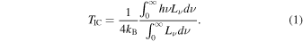
Three major theoretical models have been proposed as the origin of the disk wind in X-ray binaries; radiatively driven, thermally driven, and magnetically driven winds (see, e.g., Done et al. 2007). Radiatively driven winds can be produced when the radiation pressure is sufficiently large. As the source luminosity L approaches the Eddington limit Ledd, the "effective" gravity decreases by a factor of  Ueda et al. (2004) showed that a wind can be launched when a gas in Keplerian motion is exposed to the radiation with L > 0.5Ledd. Thermally driven winds can be launched at even lower luminosities. When X-rays from the central source heat up an upper layer of the accretion disk to the Compton temperature TIC that is higher than the gravitational binding potential at that radius, the gas will be released from the system by its thermal pressure (Begelman et al. 1983). Here, TIC is calculated from the X-ray spectra by considering the equilibrium of Compton-heating and Compton-cooling photons:
Finally, magnetically driven winds may be formed by magnetohydrodynamics effects, where magnetic field transports the angular momentum from the disk outward (Penna et al. 2010).
It is not clear whether or not all disk winds in BHBs have a common, unique origin. Previous studies suggested that most disk winds are consistent with thermally driven ones on the basis of their estimated locations (e.g., Kubota et al. 2007). By contrast, evidence for a magnetically driven wind was reported in GRO J1655−40 by Miller et al. (2006a), who found that the launching radius is much smaller than that expected from a thermally driven wind by using a diagnostic of the density sensitive lines. Uttley & Klein-Wolt (2015) demonstrated that this high-density wind appeared during a nonstandard accretion and variability state. The interpretation of this particular case is still under debate, however (e.g., Netzer 2006; Miller et al. 2008; Kallman et al. 2009; Neilsen et al. 2016; Shidatsu et al. 2016; Done et al. 2018). For instance, recent works suggest that the wind may be Compton-thick, shielding substantial intrinsic X-ray emission, and that radiative pressure may play a critical role to drive this wind. From analyses of the multi-wavelength spectral energy distribution, Neilsen et al. (2016) and Shidatsu et al. (2016) estimated the intrinsic luminosity to be several tens of times and ≳0.7 times the Eddington luminosity, assuming that the optical flux is dominated by the blackbody emission from the photosphere of the wind, and by the irradiated disk emission from the outer disk, respectively. Thus, it is very important to do more observational tests to identify the origin of disk winds.
4U 1630−47 is an ideal BHB to investigate the properties of the disk wind thanks to its brightness and frequent outbursts. Figure 1 shows the overall light curve of 4U 1630−47 obtained with the All Sky Monitor (ASM) on board the Rossi X-ray Timing Explorer (RXTE; Levine et al. 1996) and with the Gas Slit Camera (GSC) on board the Monitor of All-sky X-ray Image (MAXI; Matsuoka et al. 2009). Here the count rates of the RXTE/ASM light curve are converted to the energy fluxes by using Equation (A1) in Zdziarski et al. (2002), and those of the MAXI light curve in the 4–10 keV band are converted to the 3–12 keV fluxes by assuming the Crab spectra. As noticed, 4U 1630−47 exhibits quasi-periodic outbursts with a 600–700 day cycle. Kubota et al. (2007) detected H-like and He-like iron absorption lines from six observations in the HSS with Suzaku during the 2006 outburst (indicated by the down arrow in Figure 1). They found that these absorption lines became weaker with increasing luminosity, which is consistent with a photoionization scenario. King et al. (2014) also reported the highly ionized absorption lines during the 2012 outburst when the source was in a very similar state to those observed by Kubota et al. (2007). Hori et al. (2014) observed 4U 1630−47 in the very high state (VHS) around the peak of the 2012 outburst with Suzaku, and found that the iron-K absorption lines disappeared in this state. The absence of these features in the VHS was also reported by Díaz Trigo et al. (2014) by using the XMM-Newton data.

Figure 1. Long-term light curves of 4U 1630−47 in the 3–12 keV band obtained with RXTE/ASM (black) and MAXI/GSC (red). Two long outbursts occurred around MJD = 53,000 and MJD = 56,000. The 2006, 2012, and 2015 outbursts are indicated by the down arrows.
Download figure:
Standard image High-resolution imageIn this paper, we present the results of simultaneous observations of 4U 1630−47 with Suzaku and NuSTAR on three occasions during the 2015 outburst. A part of the preliminary results were reported in Hori et al. (2016), which should be superseded by this work. Combining with the Suzaku results in the 2007 outburst, we examine the evolution of the iron-K absorption lines in the HSS. Section 2 describes the observation and data reduction. The results of the spectral analysis are presented in Section 3. We discuss the origin of the disk wind by comparison with a theoretical model in Section 4, and summarize our conclusions in Section 5. For convenience of discussion, we always assume the distance of D = 10 kpc and inclination angle of i = 70° as reference values, which are all unknown for this target. Solar abundances by Anders & Grevesse (1989) are adopted. The errors in spectral parameters are given at 90% confidence limits for a single parameter of interest unless otherwise stated.
2. Observation and Data Reduction
Figure 2 shows blow-ups of the X-ray light curves of 4U 1630−47 during the 2006 (a), 2012 (b), and 2015 (c) outbursts. The top, middle, and bottom panels plot those in the 3–12 keV band obtained with RXTE/ASM (a) or with MAXI/GSC (b and c, converted from the 4–10 keV count rate by assuming the Crab spectrum), those in the 15–50 keV band obtained with the Burst Alert Telescope (BAT) on board Swift (Burrows et al. 2005), and their hardness ratio (3–12 keV/15–50 keV), respectively. Three ToO (Target of Opportunity) observations of 4U 1630−47 were performed with Suzaku on 2015 February 20, 24, and 27, simultaneously with NuSTAR (Harrison et al. 2013) for the first two epochs. The overall behavior of the 2015 outburst was quite complex, showing several spiky peaks around the maximum luminosity. Our ToO observations, whose epochs are indicated by the dotted lines in Figure 2(c), were made around the second peak of the outburst. The luminosity in the 2–6 keV band was the highest in the first epoch among the three, and those in the second and third ones were similar to each other (Table 1).

Figure 2. (Top) Expanded light curves of 4U 1630–47 in the 3–12 keV band during 2006 (a), 2012 (b), and 2015 (c) outburst, observed with RXTE/ASM for (a) and MAXI/GSC for (b) and (c). (Middle) Those in the 15–50 keV obtained with Swift/BAT. (Lower) The hardness ratio between the two bands. The dashed lines represent the epochs of the Suzaku observations.
Download figure:
Standard image High-resolution imageTable 1. Observation Log
| OBSID | Suzaku Observation Date | XIS Option | Exposure (ks) | Flux ( ) ) |
||||
|---|---|---|---|---|---|---|---|---|
| Start | End | Suzaku | NuSTAR | 2–6 keV | 12–30 keV | |||
| XIS | PIN | |||||||
| 6 | 2006 Feb 8 15:09 | Feb 9 3:20 | 1/4 window + 1s burst | 11.1 | 20.5 | ⋯ | 3.4 × 10⁻⁹ | 1.5 × 10⁻¹⁰ |
| 5 | 2006 Feb 15 23:29 | Feb 16 13:08 | 1/4 window + 1s burst | 10.7 | 16.0 | ⋯ | 2.5 × 10⁻⁹ | 1.2 × 10⁻¹⁰ |
| 4 | 2006 Feb 28 23:18 | Mar 1 16:43 | 1/4 window + 1s burst | 10.7 | 17.9 | ⋯ | 2.4 × 10⁻⁹ | 7.3 × 10⁻¹¹ |
| 3 | 2006 Mar 8 1:49 | Mar 8 17:31 | 1/4 window | 10.6 | 19.1 | ⋯ | 2.1 × 10⁻⁹ | 5.0 × 10⁻¹¹ |
| 2 | 2006 Mar 15 5:26 | Mar 15 17:51 | 1/4 window | 23.2 | 17.7 | ⋯ | 1.9 × 10⁻⁹ | 4.2 × 10⁻¹¹ |
| 1 | 2006 Mar 23 10:13 | Mar 23 22:21 | 1/4 window | 21.7 | 21.3 | ⋯ | 1.7 × 10⁻⁹ | 3.7 × 10⁻¹¹ |
| 8 | 2015 Feb 20 5:41 | Feb 21 9:52 | 1/4 window + 0.3s burst | 5.3 | ⋯ | 16.5a | 4.4 × 10⁻⁹ | 6.0 × 10⁻¹⁰ |
| 7 | 2015 Feb 24 1:30 | Feb 25 2:44 | 1/4 window + 0.3s burst | 5.5 | ⋯ | 16.1b | 3.7 × 10⁻⁹ | 1.4 × 10⁻¹⁰ |
| 0 | 2015 Feb 27 2:28 | Feb 28 3:42 | 1/4 window + 0.3s burst | 5.1 | ⋯ | ⋯ | 3.7 × 10⁻⁹ | ⋯ |
| α | 2012 Oct 2 0:24 | Oct 2 20:38 | 1/4 window + 1s burst | 2.9 | 39.5 | ⋯ | 6.6 × 10⁻⁹ | 3.5 × 10⁻⁹ |
Notes.
aObserved between 2015 Feb 20 11:36 and Feb 20 23:31. bObserved between 2015 Feb 24 10:46 and Feb 24 21:46.Download table as: ASCIITypeset image
Suzaku carried two types of detectors, the X-ray Imaging Spectrometer (XIS) and the Hard X-ray Detector (HXD). At the time of our observations, two front-side-illuminated XISs (FI-XISs) XIS0 and XIS3, and one back-side-illuminated XIS (BI-XIS), XIS1, were available, whereas the HXD was turned off due to the power shortage of the spacecraft. All XISs were operated with the one-fourth window mode and the 0.3 s burst option to avoid pileup effects. We utilized the "cleaned" event files reduced by the pipeline processing version 2.8.20.37 and analyzed them in a standard manner with HEASOFT version 6.16 and calibration database released on 2015 March 12. We estimated the fraction of piled-up events using the aepileupcheckup.py tool,5
and found that it could be reduced to <1% by excluding the central circular region with a radius of 0 3. Hence, the XIS spectra were integrated within an annular region with an inner and an outer radius of 03 and 13, respectively. Comparing with the spectra integrated with larger inner radii, we confirmed that the pileup effects were negligible in our spectra at energies up to 9 keV. The background spectra were taken from a circular region with a radius of 13 away from the source by 7'. Further details about these observations are listed in Table 1.
NuSTAR has two Focal Plane Modules (FPM), A and B. The NuSTAR data were reduced with the standard pipeline NUPIPELINE version 0.4.3 and were analyzed with NUSTARDAS software version 1.4.1 included in HEASOFT version 6.16. The source spectra were extracted from a central 100'' circular region around the target by using the standard tool NUPRODUCTS. We extracted the background spectra from an annular region with an inner and an outer radius of 240'' and 260'', respectively. The exposure times are listed in Table 1.
We found that the FI-XIS spectra were apparently harder than the BI-XIS spectra, most probably due to the cross-calibration error, as reported in recent Suzaku data (e.g., Shidatsu et al. 2013). Hence, these differences were approximately corrected by multiplying the FI-XIS spectra by a power-law function with a photon index of −0.10 in spectral fitting. This procedure made much better agreement of the FI spectra with the BI-XIS and NuSTAR spectra.
We reanalyzed the Suzaku archive data taken during the 2006 outburst (obsid = 400010010 through 400010060), which were analyzed and published by Kubota et al. (2007), to compare our results to those of previous Suzaku observations. The shape of the light curves (Figure 2(a)), characterized by a fast rise and a gradual decay, were less complex than that of the 2015 outburst. The right and left dashed lines in this figure represent the epochs of the first (obsid = 400010010) and the last (obsid = 400010060) observations, respectively. The details of these observations are also listed in Table 1. Because all observations in 2006 suffer from pileup effects, these spectra were extracted within an annular region with an inner and an outer radius of 1' and 17, respectively, so that the pileup fraction should be less than 1%.
Figure 3 shows the time-averaged spectra in the 2006 and 2015 outbursts. The overall spectral shapes are almost the same in these observations, except that in the brightest observation in the 2015 outburst (orange), which showed a stronger hard power-law tail. Hereafter, we refer to the first to sixth observations in 2006, the second observation in 2015, and the first one in 2015 as OBS 1 to 6, 7, and 8, respectively (in order of increasing luminosity). We refer to the third observation during the 2015 outburst as OBS 0 and treat it separately because no hard X-ray data above 10 keV are available. As an exception, the VHS observation in 2012 is referred to as OBS α. We note that the spectra in OBS 7 (blue) became slightly softer than that in OBS 6 (red). We note that the spectra of OBS 7 is very similar to the spectrum of OBS 6 taken 9 years before, except that the hard tail is slightly fainter.
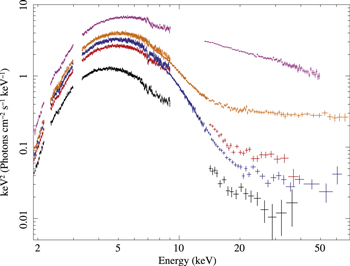
Figure 3. The broadband spectra of 4U 1630−47 in the 2006 (black and red—OBS 1 and 6), 2015 (blue and orange—OBS 7 and 8), and 2012 (magenta—OBS α) outbursts. We plot the time-averaged Suzaku/XIS1 and HXD spectra in the range of 2–9 keV and 12–40 keV, respectively. The HXD was not operated during the 2015 outburst. The NuSTAR/FMPA spectra in the 2015 outburst are also plotted, which cover the 7.5–70 keV range. The HXD was operated in the 2012 outburst (magenta) when the source was in the VHS.
Download figure:
Standard image High-resolution imageFor comparison, we also plot the VHS spectra (OBS α) observed in the 2012 outburst, which was published by Hori et al. (2014). The flux responsible for photoionization of iron ions (i.e., above ∼9 keV) in this observation was much higher than in the HSS. The spectrum did not show any iron-K absorption line feature that are ubiquitously detected in the HSS (OBS 1–8). Hori et al. (2014) showed that iron ions in the disk wind could not have been fully ionized only by the increase of photoionizing photons, if their physical parameters (location and density) had been the same as those in the HSS.
3. Spectral Analysis
3.1. Effect of Dust Scattering
Since 4U 1630−47 suffers from heavy absorption by the interstellar matter ( ), effects by the dust scattering are not negligible (Smith et al. 2002; Ueda et al. 2010). A part of the direct emission is "scattered-out" by interstellar dust in the line of sight, while photons emitted with slightly different angles from the line of sight are "scattered-in" toward the observer, producing a dust-scattering halo around the source. When the source flux and spectrum is constant, integrating all scattered-in photons will cancel the scattered-out ones, and therefore no correction is necessary. This is not the case in our data, however, because the spectrum extraction regions of Suzaku/XIS and NuSTAR/FMP do not fully cover the dust-scattering halo. Hence, we have to estimate the fraction of the dust-scattering-halo photons contained in the spectrum extraction region (hereafter "scattering fraction") and to correct for this effect in the spectral analysis.6
The situation becomes even more complex for a variable source because of the time delay between the direct and scattered-in components (see, e.g., Tiengo et al. 2010; Heinz et al. 2015, 2016).
), effects by the dust scattering are not negligible (Smith et al. 2002; Ueda et al. 2010). A part of the direct emission is "scattered-out" by interstellar dust in the line of sight, while photons emitted with slightly different angles from the line of sight are "scattered-in" toward the observer, producing a dust-scattering halo around the source. When the source flux and spectrum is constant, integrating all scattered-in photons will cancel the scattered-out ones, and therefore no correction is necessary. This is not the case in our data, however, because the spectrum extraction regions of Suzaku/XIS and NuSTAR/FMP do not fully cover the dust-scattering halo. Hence, we have to estimate the fraction of the dust-scattering-halo photons contained in the spectrum extraction region (hereafter "scattering fraction") and to correct for this effect in the spectral analysis.6
The situation becomes even more complex for a variable source because of the time delay between the direct and scattered-in components (see, e.g., Tiengo et al. 2010; Heinz et al. 2015, 2016).
In this paper, we follow the same procedures as those described in Hori et al. (2014). We estimate the scattering fraction to be 87% and 67% for the Suzaku/XIS spectra during the 2006 and 2015 outbursts, respectively, with the FTOOL xissimarfgen by assuming the image profile of the dust-scattering halo obtained by Smith et al. (2002).7
For the NuSTAR/FMP data, we approximately estimate it to be 66% by ignoring the point-spread function. Then, in the spectral fit, we utilize the Dscat model, which is a local model developed by Ueda et al. (2010), to take into account the effects of dust-scattering. We check effects by time variability of 4U 1630−47 during the 2015 observations. The maximum time delay at the outer integration radius 12 is estimated to be ∼1 day by assuming that the scatterers are located at the half distance of 10 kpc (see, e.g., Heinz et al. 2015 for the calculation). The source shows a flux decay of ∼20% around the Suzaku observations on this timescale (Figure 2(c)), which would lead to an enhancement of the scattering fraction by <4% in OBS 8. We confirm that it does not affect our final results (Section 4). Hence, for simplicity, we ignore time variability in estimating the scattering fraction in the following analysis.
3.2. Continuum Modeling
Spectral analysis is performed separately to the data of OBS 1 through 8. We use the spectra of Suzaku/XIS, Suzaku/PIN, and NuSTAR/FMP in the energy range of 1.9–9.0 keV, 12–40 keV, and 6–80 keV, respectively. Conservatively, the XIS data above 9.0 keV are not utilized to minimize pileup effects, and those in the 2.1–2.3 keV and 3.0–3.4 keV are also excluded to avoid calibration uncertainties. The spectra of the two FI-XISs (XIS0 and 3) are summed together. Spectral fitting is performed by using XSPEC version 12.8.2.
We apply a conventional model consisting of a multi-color disk (MCD) component and a power law with a low energy cutoff (diskbb and simpl in XSPEC terminology, respectively). The simpl model has two free parameters, the photon index Γ and the fraction of the seed photons fPL. To take into account adsorption by interstellar medium, we use the tbabs model with the Wilms et al. (2000) abundances and the Verner et al. (1996) cross section. To estimate the column density of iron ions in a simple manner, we utilize the "kabs" model (Ueda et al. 2004), an XSPEC local model calculating the Voigt profile from multiple fine-structure lines. The kabs model has three free parameters, the column density of each ion  , the velocity dispersion, which is fixed at 500 km s−1 in this analysis (Kubota et al. 2007), and the wind velocity v/c. The model is thus expressed as tbabs∗Dscat∗kabs∗kabs∗simpl∗diskbb in the XSPEC terminology, where the first and second kabs terms represent the absorption lines of H-like and He-like iron ions, respectively. We apply this model to all the XIS spectra in the 2006 and 2015 outbursts.
Table 2 summarizes the best-fit parameters and chi-squared value for each observation. Reasonably good fits are obtained with this model yielding the best-fit disk temperature of Tdisk ≈ 1.2–1.4 keV and photon index of Γ ≈ 2–3. For OBS 0, Γ and fPL are fixed to be 2.5 and 1.0%, respectively, because the spectrum only covered the energy range below 9 keV. During the 2006 outburst, the disk temperature and luminosity change together as expected in standard disk model to maintain a constant inner radius (Shakura & Sunyaev 1973). The inner disk radius (and column density) are slightly different in the 2015 outburst, most probably due to residual calibration uncertainties. The fraction fPL is also almost constant from OBS 1–7 at around 1%, but then increases significantly in OBS 8.
Table 2. Best-fit Parameters for Spectral Modeling
| Component | TBabs | diskbb | simpl | kabs | |||||
|---|---|---|---|---|---|---|---|---|---|
| Parameter | NHa |

|

|
Γ | fPL (%) |
 b
b
|
 b
b
|
 ) ) |
 dof dof |
| OBS 1 |

|

|

|

|

|

|

|

|
522/684 |
| OBS 2 |

|

|

|

|

|

|

|

|
539/699 |
| OBS 3 |

|

|

|

|

|

|

|

|
603/699 |
| OBS 4 |

|

|

|

|

|

|

|

|
557/696 |
| OBS 5 |

|

|

|

|

|

|

|

|
558/699 |
| OBS 6 |

|

|

|

|

|

|

|

|
576/713 |
| OBS 7 |

|

|

|

|

|

|

|

|
1422/1497 |
| OBS 8 |

|

|

|

|

|

|

|

|
1454/1497 |
| OBS 0 |

|

|

|
2.5(fixed) | 1.0(fixed) |

|

|

|
846/843 |
Notes.
aHydrogen column densities in the unit of .
bIon column densities in the unit of
.
bIon column densities in the unit of  .
.
Download table as: ASCIITypeset image
3.3. Long-term Variability of the Disk Wind
In this subsection, we focus on the iron-K absorption line features in OBS 1–8. No other line feature is significantly detected in the XIS spectra. Figure 4 shows the XIS unfolded spectra of OBS 1, 6, 7, and 8 in the 6–7.5 keV range together with the best-fit continuum model including the interstellar absorption and dust scattering. For comparison, we also plot the spectrum in the VHS (OBS α), which does not show any iron-K absorption line feature. Here we adopt the model D in Hori et al. (2014) for the continuum, which gives the best description of the Suzaku spectra. This model properly takes into account Comptonization of the inner disk emission with energetic coupling between the disk and corona, and the reflection of the Comptonized component from the accretion disk with general relativistic smearing effects. For further details, see Hori et al. (2014).

Figure 4. The unfolded spectra in the energy range of 6–7.5 keV during the 2006 (black and red), 2012 (magenta), and 2015 outbursts (blue and orange). Data of all XISs (XIS0, 1, and 3) are summed. The solid lines show the best-fit continuum model, excluding the kabs models (see the text). We also show the residuals between the data and best-fit models.
Download figure:
Standard image High-resolution imageFigure 5 plots the column density of He-like and H-like irons against the 2–6 keV flux in the HSS during the 2006 (black) and 2015 outbursts (red). OBS 1 and OBS 6 are the faintest and brightest observations in the 2006 outburst, while OBS 7 and OBS 8 are the faintest and brightest observations in the 2015 outburst, respectively. The degree of ionization of the disk wind can be traced by the ratio of the column density in H-like to He-like iron. This gradually increases with 2–6 keV luminosity in the 2006 outburst, and then increases much more rapidly in the 2015 outburst, especially in the brightest observation, OBS 8. This result might be explained by photoionization of the disk wind because the observed X-ray spectrum shows significant hardening in the brightest observation owning to the increase of the hard tail component; we will quantitatively examine this possibility in the next section. We also note that the absorption lines in OBS 6 are weaker than those in OBS 7 as expected from the harder spectrum in OBS 6.
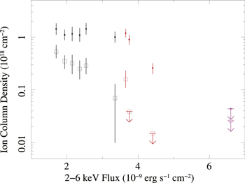
Figure 5. Correlation between the 2–6 keV flux and the column densities of iron ions obtained from the HSS spectra in the 2006 (black), 2012 (magenta), and 2015 (red) outbursts. The filled and squared dots represent the column densities of H-like and He-like iron ions, respectively.
Download figure:
Standard image High-resolution image4. Discussions
Our Suzaku and NuSTAR observations of 4U 1630−47 during the 2015 outburst confirm the presence of absorption line features of highly ionized iron ions in the HSS spectra, which were reported by previous observations in the HSS during the 2006 outburst (Kubota et al. 2007). This strongly suggests that a highly (but not fully) ionized disk wind is always present in the HSS. These data enables us to investigate the evolution of the disk wind according to the change of luminosity and spectrum from a single source in detail.
4.1. A Simple Photoionized Simulation
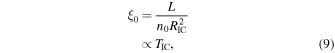
We find that the ratio between the column densities of H-like and He-like iron ions increased at fluxes above  where their spectra became harder with increasing contribution from the hard tail (Figure 3). In order to examine whether an increase of photoionizing photons solely explains the observed increase of the ionization degree or not, we perform simulations of a photoionized gas, using XSTAR version 2.3. In XSTAR simulations, the ionization parameter of the absorber at the nearest point (i.e., the launching radius for a disk wind), ξ0, is defined as
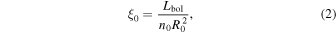
where Lbol is the luminosity in the 0.0136–13.6 keV band, R0 is the distance of the absorber from the central source, and n0 is the density. We use the observed continuum corrected for absorption and dust scattering in the 0.01–1000 keV range as the input of the source spectrum. To consider a self-similarly expanding wind with a constant velocity (Begelman et al. 1983), we assume a density (n) profile with respect to radius  as
as  , which gives an almost constant ionization parameter profile (
 ).8
The turbulent velocity is set to be
).8
The turbulent velocity is set to be  in this simulation as a representative value, which has not been measured in this source (but not less than
  Kubota et al. 2007). To directly apply the simulation results to the Suzaku/XIS spectra, we make a grid XSPEC model of absorption by utilizing the XSTAR2XSPEC tool. Through the fitting, we are able to obtain the column density
  and the ionization parameter ξ0.
We find that the higher ionization degree in OBS 8 than in the other HSS observations cannot be explained solely by the change of the source spectrum luminosity if we assume that the wind launching radius and density were the same as in the other epochs. This fact is found for the first time from 4U 1630–47, whereas similar results (i.e., that photoionization alone cannot explain changes of the ionization degree of a disk wind) were reported from other sources (Yamaoka et al. 2001 and Neilsen & Homan 2012 for GRO J1655–40, Neilsen et al. 2012 for GRS 1915+105). In OBS 8, we are able to obtain only lower limits for ξ0 and  because of the nondetection of He-like iron absorption line and of strong coupling between ξ0 and
  . If we fix the column density at
  , which is obtained in OBS 7 showing the closest luminosity to that in OBS 8 (see Table 3), the ionization parameter in OBS 8 becomes
  . This is significantly higher at a >90% confidence level than the value expected from the photoionization effect alone (i.e., the
  , which is converted from the result of OBS 7 by replacing the luminosity with that of OBS 8). This result indicates that other physical parameters of the wind, such as wind launching radius R0 and/or density at the launching radius n0, must have changed from OBS 7 to OBS 8.
4.2. Simulations of Photoionized Disk Wind
In the following, we show that these results can be explained by a theory of thermally driven winds. The Compton temperature TIC and the wind escape velocity Vwind depend on the wind launching radius (or Compton radius, RIC) as

and

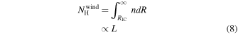
Here, k, G, and MBH are the Boltzmann constant, the gravitational constant, and the mass of the BH, respectively. From numerical simulations, Woods et al. (1996) showed that the mass flux per unit area of an isothermal disk wind,  , is given by
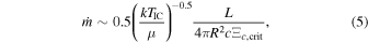
where μ, c, and Ξc,crit are the mean mass per particle, the light speed, and the critical pressure ionization parameter determined by the spectrum, respectively. The mass-loss rate of the disk wind  and the density at the base of the wind n0 given as the following equations (Done et al. 2018)
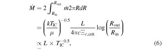
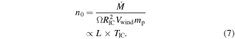
Here, Rin (Rout) is the inner (outer) disk radius, mp is the proton mass, and Ω is the solid angle of the disk wind, which is assumed to be constant against the distance from the BH. The n0 value in the OBS 1 is set to be  , which yields the mean number density of
  estimated by Kubota et al. (2007). In the following XSTAR simulations, n0 for each observation is calculated from Equation (7) (see Table 3). From these equations, we finally obtain the dependence of the column density
  and the ionization parameter at the base of wind ξ0 on luminosity and Compton temperature as
and
respectively.
Table 3. Fitting Results
| Parameter | OBS 1 | OBS 2 | OBS 3 | OBS 4 | OBS 5 | OBS 6 | OBS 7 | OBS 8 |
|---|---|---|---|---|---|---|---|---|
 a
a
|
1.20 | 1.34 | 1.48 | 1.61 | 1.63 | 2.13 | 2.61 | 3.14 |
 b
b
|
0.70 | 1.37 | 0.92 | 0.99 | 0.95 | 1.38 | 0.83 | 3.25 |
 c
c
|
1.0 | 2.1 | 1.6 | 1.9 | 1.8 | 3.5 | 2.6 | 12.0 |
log( ) ) |

|

|

|

|

|

|

|

|
|

|

|

|

|

|

|

|

|

|

|

|

|

|

|

|

|

|
Notes.
aUnabsorbed luminosities in the range of 0.0136–13.6 keV assuming isotropic emission. bCalculated by Equation (1) with the integration range of 0.01–1000 keV. cCalculated by Equation (7). n0 in OBS 1 is set to be .
.
Download table as: ASCIITypeset image
The spectral fitting results (the best-fit values and 1σ errors of  ,
,  , and Vwind) are summarized in Table 3 along with the luminosity L, Compton temperature kTIC, and the density n0 assumed in the XSTAR simulations. Figures 6(a) and (b) plots NHwind against L, and ξ0 against kTIC, respectively. Only lower limits of
  and ξ0 are obtained in OBS 8 (orange arrows).

Figure 6. (a) The Lbol dependence of the ion column density  and (b) the TIC dependence of the ionization parameter ξ0. The black, red, and blue points represent the spectral fitting results (with 1σ errors) for OBS 1–5, 6, and 7, respectively. We only obtain the lower limit with OBS 8 (orange) due to the nondetection of the He-like iron absorption line. The green solid lines in (a) and (b) show the best-fit relation of Equations (8) and (9), respectively. The light green regions correspond to the 90% confidence interval. The orange dashed curve plots the best-fit ionization parameter by assuming a column density of
  . The magenta dashed arrows represent the lower limits for the VHS spectra in 2012 with an assumption of
  .
.
Download figure:
Standard image High-resolution imageWe have confirmed that correlation between  and L is significant at a 95% confidence level, by performing an F-test between the cases when we fit those data with a constant and with a linear function. The linear fit yields a slope of 0.67 ± 0.25 and a y-intercept of 0.23 ± 0.39, which is consistent with zero. Accordingly, we fit the data again by assuming Equation (8) (i.e., proportional relation). The best-fit line with the 90% confidence interval is plotted in Figure 6(a), showing that all the data in OBS 1 through 8 are consistent with the theoretical relation. On the basis of our disk wind model, we are able to estimate the ionization parameter in OBS 8 to be
  through the spectral fit, by adopting
  predicted from Equation (8). This result is plotted in the orange dotted line in Figure 6(b). By including this data point, correlation between ξ0 and TIC is also confirmed at a 91% confidence level via an F-test. The best-fit relation of Equation (9) is plotted in Figure 6(b), with which all the data are consistent. We note that the possible increase of the scattering fraction in OBS 8 (discussed in Section 3.1) does not affect our final results. The maximum increase of the scattering fraction (4%) leads to an only ∼1% luminosity decrease and a ∼2% Compton temperature increase.
The nondetection of the iron-K absorption lines in the VHS during the 2012 outburst does not contradict this theory. The column density and ionization parameter are predicted to be  and
and  by using
  and
and  with Equations (8) and (9). Analyzing the VHS spectra in the same way as for the HSS data, we obtain a lower limit of the ionization parameter of ξ0 > 5.38 at a 99% confidence level. This is still consistent with the theoretical prediction (see Figure 6(b)). We do not rule out, however, the possibility that the geometrical configuration between the central source and outer disk might have changed in the VHS, leading to a more efficient ionization of the disk wind in the VHS than in the HSS. We note that runaway ionization of the wind via thermodynamical instability is unlikely to occur in the VHS (Chakravorty et al. 2013).
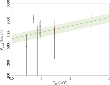
Figure 7 plots the relation between the wind velocity Vwind and the Compton temperature TIC in the 2006 outburst. We find that the correlation is not statistically significant in our data, which are subject to large uncertainties. Nevertheless, the green line, representing the best-fit relation of  (see Equation (4)), is consistent with the observed data except for OBS 7. We note that Vwind has a systematic error of ∼200 km s−1 due to a possible energy-gain uncertainty of Suzaku/XIS, which became larger in the 2015 observations (OBS 7 and 8).9
Figure 7. Relation between the best-fit wind velocity Vwind (with 1σ errors) and the Compton temperature TIC. The black, red, blue, and orange points show that of OBS 1 to 5, 6, 7, and 8, respectively. The green line shows the best-fit relation of Equation (4) with the 90% confidence interval. We note that there are systematic errors of ≳200 km s−1 in Vwind due to calibration uncertainties.
Download figure:
Standard image High-resolution image
From these results, we conclude that the evolution of the observed iron-K absorption line features in the spectra of 4U 1630–47 are consistent with a simple theory of thermally driven disk winds. We have shown that it is important to consider the dependence of the launching radius of a disk wind on the Compton temperature TIC, which is determined by the shape of the continuum. Further observational studies with high-resolution spectroscopy that enable us to more accurately determine the outflow velocity would be useful to confirm our scenario.
Although the data and model agree fairly well, there are potential uncertainties in our calculation; here we assumed very simple velocity/density structures to predict the observable of thermally driven wind. Also we ignored the reduction of RIC by radiation pressure, which becomes significant above ∼0.3LEdd (Done et al. 2018). Hydrodynamic simulations and radiation transfer calculation based on their results would be required for more accurate discussion, which we left for future work.
5. Conclusions
We performed three observations of 4U 1630−47 with Suzaku during the 2015 outburst, simultaneously with NuSTAR in the first two epochs. For comparison, we also reanalyze the Suzaku data taken during the 2006 and 2012 outburst. The conclusions are summarized below.
- 1.The continuum in the HSS is well described by thermal disk emission and a weak power-law tail produced by Comptonization of the disk photons. The K absorption lines from highly ionized iron ions are detected in all observations in the HSS during the 2006 and 2015 outbursts.
- 2.We investigate the evolution of the disk wind parameters as a function of luminosity and spectrum. The degree of ionization dramatically increased at the brightest state during the 2015 outburst. The XSTAR simulations show that this change cannot be explained solely by photoionization effects if we assume constant launching radius and density of the wind.
- 3.We find that a simple theory of thermally driven winds can explain our observational results. We point out that the thermal disk winds respond to changes in the illuminating source flux and spectral shape. These parameters change the launch radius and density of the wind, which also affect its photoionization state.
We thank Fiona Harrison for approving our request for ToO observations of NuSTAR and the Suzaku and NuSTAR operation teams for scheduling the simultaneous observations. Part of this work was financially supported by the Grant-in-Aid for JSPS Fellows for young researchers (T.H.) and for Scientific Research 17K05384 (Y.U.). C.D. acknowledges STFC funding under grant ST/L00075X/1 and a JSPS long-term fellowship L16581. M.S. acknowledges support by the Special Postdoctoral Researchers Program at RIKEN.
Footnotes
- 5
- 6
In reality, the effect of the point-spread function must also be taken into account for both direct and halo components.
- 7
We have confirmed that our results on the disk wind parameters do not change beyond the errors by adopting a different halo profile presented in Smith et al. (2016).
- 8
Here we adopt an index of −1.9 instead of −2.0 for the density profile because XSTAR calculations do not converge if we set n ∝ R−2 due to technical reasons. We have confirmed that our results are little affected by its choice within a range between −1.5 and −1.9.
- 9