


Abstract
The velocity oscillations observed in the chromosphere of sunspot umbrae resemble a resonance in that their power spectra are sharply peaked around a period of about three minutes. In order to describe the resonance that leads to the observed 3-minute oscillations, we propose the photospheric resonator model of acoustic waves in the solar atmosphere. The acoustic waves are driven by the motion of a piston at the lower boundary, and propagate in a nonisothermal atmosphere that consists of the lower layer (photosphere), where temperature rapidly decreases with height, and the upper layer (chromosphere), where temperature slowly increases with height. We have obtained the following results: (1) The lower layer (photosphere) acts as a leaky resonator of acoustic waves. The bottom end is established by the piston, and the top end by the reflection at the interface between the two layers. (2) The temperature minimum region partially reflects and partially transmits acoustic waves of frequencies around the acoustic cutoff frequency at the temperature minimum. (3) The resonance occurs in the photospheric layer at one frequency around this cutoff frequency. (4) The waves escaping the photospheric layer appear as upward-propagating waves in the chromosphere. The power spectrum of the velocity oscillation observed in the chromosphere can be fairly well reproduced by this model. The photospheric resonator model was compared with the chromospheric resonator model and the propagating wave model.
Export citation and abstract BibTeX RIS
1. Introduction
Three-minute oscillations of intensity and velocity are commonly noticeable in the chromosphere of sunspot umbrae. Even though these three-minute umbral oscillations have mostly been observed through chromospheric lines such as the Ca ii H and K lines (e.g., Beckers & Tallant 1969), Hα (e.g., Giovanelli 1972), the Ca ii IR triplet (e.g., Lites et al. 1982), Na i D1 and D2 (e.g., Kneer et al. 1982), the He i λ10830 line (e.g., Lites 1986), and the Mg ii h and k lines (Gurman 1987), the oscillations have been identified from photospheric lines as well (Lites & Thomas 1985; Stangalini et al. 2012; Chae et al. 2017). There has been increasing evidence that the three-minute oscillations observed in the chromosphere represent the slow magnetoacoustic waves that propagate upward in the gravitationally stratified medium (e.g., Brynildsen et al. 2004; Centeno et al. 2006; Felipe et al. 2010; Tian et al. 2014; Cho et al. 2015). Khomenko & Collados (2015) presented a comprehensive review of the relevant observations, analytical theories, and numerical simulations of the oscillations and waves in sunspots, providing an updated picture for understanding sunspot oscillations.
The most important property of the three-minute oscillations is the presence of peaks in the power spectrum of the velocity or intensity. The spatiotemporally averaged spectrum usually displays multiple peaks that are closely spaced in frequency, but when they are spatially and temporally well resolved, each power spectrum has a single peak (e.g., Brynildsen et al. 2003; Centeno et al. 2006; Chae et al. 2017, 2018). The physical origin of this peak is not yet resolved, even though a great number of theoretical models have been put forward. The proposed models may be categorized as the model of internally excited acoustic waves, the propagating wave model, and the resonator model. We briefly review these models below.
Acoustic waves in an atmosphere are subject to the acoustic cutoff arising from gravitational stratification (Lamb 1932). The concept of the acoustic cutoff is unambiguously established in an isothermal atmosphere, where the acoustic waves of frequencies higher than the acoustic cutoff frequency, which is often called Lamb frequency, can propagate, carrying wave energy, while the waves of lower frequencies cannot propagate. Acoustic waves may be internally excited by a localized disturbance inside the atmosphere (Lamb 1909; Kalkofen et al. 1994; Chae & Goode 2015). Chae & Goode (2015) showed that the waves of frequencies above the cutoff are generated with higher frequency waves moving out of the source region at faster group speeds, while lower frequency waves linger there for a while because of slow group speeds. After a while, the region oscillates with frequencies that are very close to the cutoff frequency, which is often called a wake. The power spectrum of the oscillation becomes sharply peaked around the cutoff if the spatial extent of the impulsive disturbance is large enough. This model of acoustic waves that are internally excited in an isothermal atmosphere, however, may not be applicable to the three-minute oscillations that are commonly observed in the solar atmosphere. Even though the impulsive disturbances that lead to 3-minute oscillations were reported by Kwak et al. (2016) and by Song et al. (2017), there is no observational evidence that such events occur inside the atmosphere frequently enough to explain the observed predominant oscillations.
Recent observations (Chae et al. 2017; Cho et al. 2019; Kang et al. 2019) rather support the notion that the sources of excitation are located below the atmosphere, as has commonly been modeled by the piston motion at the bottom of the atmosphere in previous theoretical studies (e.g., Fleck & Schmitz 1991; Kalkofen et al. 1994; Sutmann & Ulmschneider 1995). These studies found that regardless of the specific form of the piston driving, the oscillations with a frequency close to the cutoff prevail in high altitudes of the atmosphere. This oscillation frequency has often been regarded as the natural frequency of the atmosphere resulting from a resonant response or free atmospheric oscillations (Fleck & Schmitz 1991; Kalkofen et al. 1994). Chae & Goode (2015), however, made it clear that this "resonant" response is not like the resonance in a resonant cavity, but is simply due to the combined effect of the acoustic cutoff and the driving power spectrum. If the driving power spectrum is peaked at a frequency below the cutoff and decreases with frequency above the cutoff, only the waves with a frequency above the cutoff become propagating waves, and the waves with a lower frequency become evanescent waves that cannot carry wave energy. As a result, the oscillation spectrum at a high altitude is found to be peaked around the cutoff. This is the propagating wave model. This propagating wave model can provide another explanation of the peak frequency in the observed three-minute oscillations. Note that this model has originally been developed for an isothermal atmosphere, and was applied to real observations by Centeno et al. (2006). The real solar atmosphere, however, is not isothermal, which poses a problem in the propagating wave model.
The nonisothermal nature introduces further complexity in the acoustic waves in the solar atmosphere. Even though there have been studies of its effect on the propagation of waves (e.g., Sutmann & Ulmschneider 1995), its full understanding requires a careful investigation of the properties of acoustic waves. In a nonisothermal atmosphere, the acoustic cutoff frequency is not even uniquely defined, and its physical interpretation is not so simple as in an isothermal atmosphere. Chae & Litvinenko (2018) defined the acoustic cutoff frequency of a nonisothermal atmosphere as the lower limit of the frequencies where both pressure fluctuation and velocity fluctuation become oscillatory with height. The cutoff frequency of a temperature-decreasing layer is then found to be equal to the Lamb frequency at the bottom, and that of a temperature-decreasing layer is determined not only by the Lamb frequency at the bottom, but also by the temperature gradient. They also found that the acoustic cutoff frequency in a nonisothermal layer does not sharply separate the propagating wave solution and the nonpropagating wave solution, but marks the center of the frequency band where the transition from low acoustic transmission to high transmission takes place.
A real solar atmosphere is more complex than either the temperature-increasing layer or the temperature-decreasing layer, being characterized by the presence of a temperature minimum region. Typically, temperature decreases with height in the photosphere and reaches the minimum in the temperature minimum region, and increases with height in the chromosphere. This temperature structure together with density stratification may introduce wave reflection inside the atmosphere, and hence may cause resonance to occur, which has motivated the investigators to devise various models of resonant cavities or resonators in order to account for the resonant periods in the umbral oscillations. They include the Alfvén wave atmospheric resonator (Uchida & Sakurai 1975), the fast-wave photospheric resonator (Scheuer & Thomas 1981; Thomas & Scheuer 1982), the slow-wave atmospheric resonator (Leibacher & Stein 1981), the slow-wave chromospheric resonator (Zhugzhda & Locans 1981; Zhugzhda et al. 1983; Gurman & Leibacher 1984; Settele et al. 2001), the fast-wave subphotospheric resonator (Zhugzhda 1984), and the slow-wave subphotospheric resonator (Zhugzhda 1984).
The chromospheric resonator model has received much more attention than the other resonator models. It predicts a series of peaks in the power spectrum that are closely spaced (about 1 mHz interval) in frequency. According to Zhugzhda (2007), the lowest frequency originates from the temperature plateau, and the next lowest frequency from the cutoff frequency of the temperature minimum. The higher frequency peaks originates from the temperature structure of the atmosphere.
Staude et al. (1985) calculated the oscillations using the chromospheric resonator model, and showed that the observed spectrum of resonant peaks in the velocity and intensity of transition region lines observed by the Solar Maximum Mission (SMM) spacecraft can be well explained by a gradient model of the umbral chromosphere. From the SMM observations of the Mg ii k and h lines, Gurman (1987) detected the intensity oscillations that are characterized by three distinct peaks in the power spectra averaged over sunspot umbrae. He showed that the frequencies of these peaks agree well with the first three peaks predicted by the chromospheric resonator model. Christopoulou et al. (2003) detected three oscillating modes in the umbral oscillations that were simultaneously observed in the Hα and the Fe i λ5576 line and suggested that the lowest frequency peaks are due to the photospheric resonator, while the two higher frequency peaks are due to the chromospheric resonator.
Botha et al. (2011) presented the results of numerical simulation of slow magnetoacoustic waves in an umbral model atmosphere that was excited by a velocity pulse beneath the photosphere. The chromosphere acts as a leaky resonator and the power spectrum of the velocity in the chromosphere has multiple peaks—at the frequency that corresponds to the acoustic cutoff of the temperature minimum at the higher frequencies. This finding supports the chromospheric resonator model.
Brynildsen et al. (2003, 2004), however, found that the power spectra of extreme ultraviolet (EUV) intensity above each sunspot umbra are characterized by one dominant peak that corresponds to a period of three minutes, and concluded that there is no indication of resonance frequencies that would be equally spaced (1 mHz), as predicted by the chromospheric resonator model. Meanwhile, Zhugzhda & Sych (2014) analyzed the 6 hr run of He ii λ304 intensity over a sunspot umbra and obtained a very complex power spectrum with a dozen peaks. The problem posed by this observation is that the peaks are too numerous to be explained by the chromospheric resonator model. This model gives rise to only a few peaks, not a dozen. Thus it was concluded by Zhugzhda & Sych (2014) and Zhugzhda (2018) that in addition to the chromospheric resonator, a subphotospheric resonator is needed to explain the observation.
Khomenko & Collados (2015) noted that granting that a power spectrum has multiple peaks as seen in spatiotemporally averaged data, explaining these peaks using a resonator model is not easy. Primarily, the precise positions of the peaks change significantly from one observation to another, and even in time within the same observational sequence. This led Khomenko & Collados (2015) to conclude that there is no strong observational support for an umbral resonance cavity model of any kind. By employing numerical simulations of wave propagation, Felipe (2019) investigated the propagating wave model and the chromospheric resonator model together, and concluded that the propagating wave model can explain the dominant period of the three-minute oscillations even without the chromospheric resonator, but the chromospheric resonator strongly enhances the power of the three-minute oscillations if it exists.
In this paper, we propose an alternative model as the physical origin of the peak frequency in the umbral oscillations. It is the photospheric resonator model of acoustic waves. This model is similar to the chromospheric resonator model and the subphotospheric resonator model in that the temperature minimum region plays an important role as a reflecting interface. The temperature minimum region reflects the waves of lower frequencies and transmits the waves of higher frequencies. Because wave driving is very likely to occur below the temperature minimum, a frequency-depending resonator cannot but be formed between the temperature minimum and the driving position. We set the wave driving near the bottom of the atmosphere. Thus the resonator basically spans the photosphere, having a thickness of a few hundred kilometers, being much smaller than the thickness of the subphotospheric resonator (Zhugzhda 1984), which is a few thousand kilometers.
The photospheric resonator is a leaky resonator in that the resonant oscillations escape it. In the chromosphere, the photospheric resonator model is very like the model of simple propagating waves because waves propagate upward there in both the models. An idea similar to our photospheric resonator was previously proposed by Taroyan & Erdélyi (2008), but a detailed investigation of its physical concept and the comparison with specific observations was not reported.
We show that the photospheric resonator can successfully reproduce the oscillation power spectrum that is characterized by a single peak. We also compare the photospheric resonator model with the chromospheric resonator model and the propagating wave model.
2. The Physical Picture of the Photospheric Resonator
Figure 1 presents an example of velocity oscillations that are observed in the Na i D2 line, which forms in the low chromosphere above a point inside a sunspot. The detailed description and the first analysis of the data were presented by Chae et al. (2017). The figure indicates that the three-minute velocity oscillation in the low chromosphere seen through the Na i line is characterized by the presence of a single dominant peak in the power spectrum. In this case, the frequency is around 6.1 mHz, which corresponds to a peak period of 2.7 minutes.
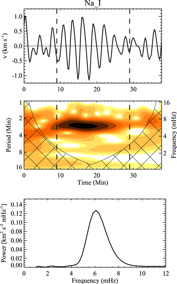
Figure 1. Plots of velocity oscillations measured inside a sunspot from the Na i D2 line, and its wavelet power spectrum and global wavelet power spectrum. The two vertical dashed lines indicate the start and end of the wave duration. The temporal average of the wavelet power spectrum over the wave duration yields the global wavelet power spectrum.
Download figure:
Standard image High-resolution imageFigure 2 presents the graphical illustration of the model of a photospheric resonator. In this model, the atmosphere consists of two nonisothermal layers: the photospheric layer, and the chromospheric layer. Temperature rapidly decreases with height in the photosphere, and slowly increases with height in the chromosphere. The interface between the two layers is the temperature minimum.

Figure 2. Illustration of the photospheric resonator. The waves of frequencies around ω1 are partially reflected by the interface at the temperature minimum.
Download figure:
Standard image High-resolution imageIn our previous work (Chae & Litvinenko 2018, hereafter Paper I), we have defined the acoustic cutoff frequency in a nonisothermal atmosphere as the frequency separating the spatially oscillatory waves and the nonoscillatory waves. The acoustic waves of the cutoff frequency are partially transmitted and partially reflected. In a temperature-decreasing layer like the photospheric layer, the acoustic cutoff frequency is equal to the Lamb frequency specified by the sound speed c0 at its bottom,

where γ is the specific heat ratio, and g is the gravitational acceleration. In contrast, in a temperature-increasing layer like the chromospheric layer, the acoustic cutoff frequency is affected by the temperature gradient as well; it is slightly higher than the Lamb frequency specified by the sound speed c1 at its bottom,

Note that the acoustic cutoff frequency of the chromosphere is close to ω1 because the chromospheric layer in our model is close to an isothermal layer.
Our model implies ω0 < ω1. Therefore it is expected that the waves of ω ≪ ω0 exist only in the interior because the bottom of the photospheric layer does not transmit them into the photospheric layer. The interface, i.e., the temperature minimum region, plays the role of the reflecting top of the photospheric layer. It fully reflects back the low-frequency waves of ω ≪ ω1. The waves of ω ∼ ω1 are partially reflected back, which causes the interference of the progressive waves and the regressive waves, and the resonance with the waves driving at frequencies near ω1. As a result, both the progressive waves and regressive waves are amplified, and the progressive waves leaking out of the interface contain large power at frequencies near ω1. Note that because the reflection is partial, the power of the progressive waves should be larger than that of the regressive waves, and a net upward flux of wave energy exists even inside the photospheric resonator. In contrast, the interface little reflects the waves of ω ≫ ω1 so that resonance does not take place. Consequently, the power of the progressive waves in the chromosphere may be small at ω ≫ ω1 unless the power of wave driving in the photosphere is strong at these frequencies.
An important assumption of the photospheric resonator we propose is that there exists a lower boundary where the velocity is no longer determined by the internal dynamics of the resonator, but is externally controlled, being prescribed by a piston motion. The location of the wave driving can be parameterized by its temperature T0 because the temperature monotonically increases with depth in the photosphere and in the interior.
3. Multilayer Modeling of Acoustic Waves in a Nonisothermal Atmosphere
3.1. Equilibrium Model
We consider an atmosphere that is in hydrostatic equilibrium,

and consists of several layers. The gravitational acceleration g is assumed to be constant. As is well known, the sound speed c is related to pressure p, density ρ, and temperature T,

with  , where kB is the Boltzmann constant, μ is the mean molecular weight, and mH is the hydrogen mass.
One can freely choose the reference pressure pr that specifies the reference atmospheric level, and the corresponding sound speed cr at the reference level. By introducing the scale length

which is equal to twice the local pressure scale height at the reference level, we define the reduced height,

which is measured from the reference level. Note that we measure the geometrical height z from this reference level as well. In the special case of an isothermal atmosphere, h is equal to z.
In Paper I we have considered the wave solution in a simple layer where dc2/dh is constant. We generalize this condition to the multilayer atmosphere. We require that it is constant in each layer indexed by l and is specified by the dimensionless parameter κl, which is defined as

for hl ≤ h < hl + 1, where hl refers to the bottom of the lth layer, and cl is the sound speed there. This equation is integrated to give

By combining Equations (3), (5), (6), and (8), we obtain the relationship between h and z:
which is integrated to give
and, after inversion
3.2. Wave Solution in Each Layer
The general solution for the linear acoustic waves can be easily constructed using the principle of superposition. We express pressure fluctuation and velocity fluctuation for each layer indexed by l as


using the complex wave functions ψω (h; l) and φω (h; l) that are written as


where fω (h; l) and gω(h; l) in general represent the progressive components of pressure fluctuation and velocity fluctuation, respectively, and their conjugates  and
and  , the regressive components. The reflection coefficient rω,l is the coefficient ratio of the regressive component to the progressive component.
Note that Equations (12) and (13) are similar to Equations (18) and (19) of Paper I, but are different from these in that Equations (12) and (13) are the full Fourier transform representation, while Equations (18) and (19) of Paper I are a simple summation representation. This difference mostly accounts for the difference in the formulae and expressions between the current work and our previous one in Paper I.
According to Paper I, in the lth layer, the coefficients Cl and Dl are related to each other as

Following Paper I, we change the independent variable h in the lth layer into a new dimensionless variable ζ that is related to ω, h and l,

with the Lamb frequency at the bottom of the lth layer

and a dimensionless parameter al defined as
where sl is the sign of κl. Note that al depends on ω as well as κl and ωl. It is obvious that the value of ζ at the bottom of the lth layer (h = hl) is given by
and after some arrangements, one can show that ζ at the top of the same layer is given by
Note that h is continuous across the interface between the lth layer and l + 1th layer, but ζ is not in general:  unless al = al + 1.
It has been shown in Paper I that the equation describing the function f(ζ) = fω(h; l) is given by

and the progressive solution representing the waves propagating upwards is given by

with two real function fJ and fY that can be expressed in terms of Bessel functions and modified functions. These two functions can also be expressed in terms of the Airy functions:


Note that fJ is a real function that behaves like a sine function at ζ > 0, and fY is a real function that behaves like a negative cosine function (see Figure 4 of Paper I). Once f(ζ) is determined, gω(h; l) = g(ζ) can be determined from fω using the equation

The behavior of the functions f(ζ) and g(ζ) at three different regimes can be conveniently investigated using the asymptotic expressions
and

with

3.3. Interface and Boundary Conditions
We consider the atmosphere composed of L layers. At the interface h = hl+1 between the lth layer and the l + 1th layer, both ψω and φω should be continuous:
for l = 0, .., L − 2. We also impose the top boundary condition that only progressive waves exist in the top layer indexed by l = L − 1:

and the bottom boundary condition that the velocity at the bottom is given by

where φω (h0; 0) is related to v (h0, t; 0) by the equation

which has been derived from Equation (13).
In order to model a pulse of finite duration, we consider the propagation of the wave packet produced by the vertical displacement of the form
corresponding to the velocity of a piston
at the low boundary. According to this velocity model, the piston is at rest at  , is accelerated downward, and reaches the maximum displacement ξ0 at t = t0 with zero velocity. After this, the piston is accelerated upward, and reaches the original equilibrium position at
  . The disturbance is characterized by the maximum displacement ξ0 and the dynamic timescale of the pulse tp.
By inserting this model into Equation (34), we obtain the expression of φω (h0; 0)
4. Theoretical Results from a Two-layer Model
4.1. A Two-layer Model Approximation
Figure 3 presents the plot of  versus h/Hr constructed from the values of pressure and density in the mean umbral model of Maltby et al. (1986). Here we set the reference level of h = z = 0 at the surface where the optical depth at 500 nm is unity. The normalizing parameters cr and Hr were calculated with pressure and density at this reference level.

Figure 3. Plots of sound speed square c2 (i.e., proportional to temperature) vs. reduced height h constructed from the umbral model of Maltby et al. (1986).
Download figure:
Standard image High-resolution imageThe figure clearly indicates that c2 rapidly decreases with h in the photosphere, and then very slowly increases with h in the chromosphere. We find that this variation can be fairly well approximated by a two-layer model K0 = −1.44 and K1 = 0.04 with the interface of  being at h1/ Hr = 0.2, where Kl is the dimensionless gradient in the lth layer, defined by
From Equations (7) and (38), we obtain the relationship
which indicates κ1 = K1/0.8 = 0.05.
The bottom of the photospheric layer is regarded as a free parameter of the model. To specify it, we introduce the dimensionless parameter
which is equal to the ratio of temperature T0/T1 when γ R is constant. Once τ is known, we can calculate c0, and hence κ0 using Equation (39). Then by inserting l = 0, c = c1, and h = h1 into Equation (8) and by solving it for h0, we obtain

In addition, by inserting l = 0, h = z = 0 into Equation (10) and by solving it for z0, we obtain the expression

and by inserting l = 0, h = h1, z = z1 into Equation (10) and by solving it for z1, we obtain the expression

4.2. Acoustic Cutoff and Transmission Efficiency of the Chromospheric Layer
In our two-layer model, the chromospheric layer is a simple nonisothermal layer where waves propagate upward. There are no regressive waves in this layer. In Paper I we have considered the acoustic transmission efficiency of a simple nonisothermal layer where only progressive waves exist. The transmission efficiency Tω of such a layer was defined by the ratio of the wave flux to the maximum value that can be realized when pressure and velocity fluctuations are perfectly correlated. Because the upper chromospheric layer indexed by l = 1 is a temperature-increasing layer where only progressive waves exist, its acoustic cutoff frequency is given by

which is equal to 1.03ω1. According to Paper I, the transmission efficiency of this layer is given by

Figure 4 presents the plot of Tω versus ω. We find from the figure that there is a smooth transition of Tω from zero to unity at frequencies around ωac and the waves transport energy even at frequencies lower than ωac. This is the property of the acoustic cutoff in a nonisothermal layer, which was reported in Paper I.

Figure 4. Plot of the transmission efficiency Tω of the upper layer. The vertical blue dashed line refers to the Lamb frequency ω1, which corresponds to c1, and the vertical red dotted line refers to the acoustic cutoff frequency ωac. Note that Tω is above zero even at frequencies below ω1 and ωac, which is a characteristic of the nonisothermal layer.
Download figure:
Standard image High-resolution imageNote that Tω is the property of the layer. It is wholly determined by the parameters ω1 and κ1 of the upper layer, and is not at all affected by the parameters of the lower layer. In contrast, the reflection coefficient to be discussed in the following is the property of the interface, characterized by the difference in the parameters between the lower layer and the upper layer.
4.3. Reflection at the Interface
In the case of the two-layer model with L = 2, one can derive from Equations (30)–(32) the expression of the reflection coefficient rω,0 in the lower layer:
with the magnitude and phase defined by

Figure 5 presents the plots of rω,0 computed using Equation (46) as a function of ω. The plots indicate that  rapidly decreases with ω at frequencies around ω1. We find from the figure that
  is anticorrelated with Tω. Note that rω,0 depends on the parameters of the lower layer but Tω does not. Thus, the strong anticorrelation between
  and Tω may be understood only if they are very sensitive to the parameters that commonly affect both. The comparison of Figures 4 and 5 suggests that both the parameters are very much affected by the acoustic cutoff frequency of the chromospheric layer ωac , which is practically determined by the minimum temperature of the atmosphere.

Figure 5. Plots of the absolute value (solid black curve) and phase (dashed curve) of the reflection coefficient rω,0 as functions of ω. The vertical blue dashed line refers to the Lamb frequency ω1, which corresponds to c1, and the vertical red dotted line refers to the acoustic cutoff frequency ωac.
Download figure:
Standard image High-resolution imageTo understand how rω,0 depends on the parameters of the two layers, we examine Equation (46) in the special case of ω = ω1. This choice leads to the following expressions: ζ(ω1, h1; 0) = ζ(ω1, h1; 1) = 0,  , and
, and  . It then follows that fω1 (h1; 0) = 1.2299i, fω1 (h1; 1) = −1.2299i,
  , and
, and  . After some algebra, we obtain the expression

with the parameter

Figure 6 presents the plots of the magnitude  and phase θr of c calculated with ω = ω1 is calculated as functions of q using Equation (48). The figure clearly indicates that both
  and θr decrease with q. The lower the value of q, the stronger the reflection. This means that for a fixed K1, a high value of
  causes strong reflection at the interface. Namely, the more rapidly the temperature decreases with height in the photosphere, the more strongly are the waves reflected at the temperature minimum.

Figure 6. Plots of the amplitude  and phase θr of the reflection coefficient as functions of the atmospheric model parameter q at the frequency ω = ω1.
Download figure:
Standard image High-resolution imageAn important point is that q only weakly depends on K1/K0. In the specific model we consider, K0 = −1.44 and K1 = 0.04, so that we have q = 0.30. Even if K1/K0 were to increase or decrease by a factor of 2, the range of q would be confined to the range from 0.24 to 0.38, in which case  would be still in the range from 0.63 to 0.73, little deviating from the value of 0.68 calculated with the specific model. Therefore we conclude that the reflection coefficient is only weakly affected by the specific structure of the atmospheric model. It is primarily determined by ω1.
It is interesting that the reflection coefficient  is completely determined by one parameter q or by the ratio K1/K0. From this result we expect that rω,0 at other frequencies is also controlled by K1/K0. This can be explicitly demonstrated for ω close to ω1 when the asymptotic formula for f(ζ) yields a correction to the reflection coefficient rω,0, which is on the order of
  . Thus the dependence of rω,0 on
  and
and  is indeed relatively weak. It is somewhat simpler to analyze the dependence of rω,0 on ω if it is expressed in terms of the function f(ζ) and its derivatives:
This form makes it obvious, for instance, that  when q = 0, as expected physically.
4.4. Resonance in the Photospheric Layer
The reflection at the temperature minimum produces the regressive waves, and the interference between the regressive waves and the progressive waves at the bottom of the photospheric layer results in a resonance at a specific frequency. Thus the photospheric layer plays the role of a resonator. We assume that the bottom of the photospheric resonator is subject to a piston driving, and its velocity can be set to a prescribed complex function φω (h0; 0) as in Equation (37). Then from Equation (33), one can derive the amplitude coefficient D0:

where D0,0 is the value of D0 in the limiting case of no reflection given by

and θ0 is the phase angle of gω (h0; 0) defined by

Therefore
which indicates that if  is not zero and is constant over ω, the amplitude
  has a local peak at the frequency ωM satisfying the condition

with which it follows cos(θr − 2θ0) = −1. This peak represents the resonance of the waves resulting from the interference between the progressive waves and regressive waves. Note that because  in fact varies with ω, the resonance frequency of Equation (54), denoted by ωR, will actually differ from ωM.
Figure 7 presents the plots of  as a function of ω and indicates the values of ωR and ωM in the three different cases of τ. Each resonance frequency ωR lies lower than the corresponding ωM because
  decreases with ω. The figure clearly shows that the higher value of τ corresponds to a lower value of ωR and a sharper peak of
  . The values of ωR/ω1 are 1.32, 1.07, and 0.98 for τ = 2.0, 2.5, and 3.0, respectively. It also should be noted that the resonance frequency ωR has a value close to ω1 in all cases.

Figure 7. Plots of normalized amplitude coefficient square  in the photospheric layer as functions of frequency ω in the different cases of the model parameter τ. The symbols mark the resonance frequency ωR and the peak values. The vertical lines mark the value of ωM/ω1 satisfying Equation (55).
Download figure:
Standard image High-resolution image4.5. Energy Spectra and Flux Spectra
The time-averaged energy of the waves  at a height h is given by

where twv is the duration of the wave packet or the length of the time interval where the velocity fluctuation has an amplitude significantly above zero. In the same way, the time-averaged flux of the wave energy is given by

By applying Parseval's theorem and making use of the fact that the amplitude is an even function of ω, we obtain
and

These expressions lead us to define the energy spectrum, velocity power spectrum, and flux spectrum as follows:


By inserting Equations (14) and (15), and making use of Equation (16), we obtain the expressions


This formula for flux spectrum Fω is derived making use of the relationship3

which results from the Wronskian formulae for the Airy functions.
Note that Eω in Equation (63) depends on h and l. Figure 8 shows the plots of Eω calculated using Equation (63) at different heights in the specific case of τ = 2.5. We find from Figure 8 that a slight enhancement of Eω(h)/Eω(h0) over unity is detected around the resonance frequency ωR near the bottom of the photospheric resonator. The strength of the energy enhancement increases with height, and reaches a peak at the top of the resonator h/Hr = 0.20. The strength decreases with height at the upper heights h/Hr > 0.2. Thus the photospheric resonator has a node at its bottom end (h/Hr = −0.63), and an antinode at its top (h/Hr = 0.20). Figure 8 also shows that the energy spectra are affected by the acoustic cutoff. At low frequencies ω, Eω(h)/Eω(h0) decreases with height and becomes much smaller than unity at heights h/Hr > 0.20. As a consequence of this cutoff, the profile of Eω(h)/Eω(h0) at a large height, i.e., h/Hr = 2.52, appears asymmetric over ω, rapidly increasing with ω for ω ≲ ω1 and slowly decreasing with ω for ω > ω1.

Figure 8. Plots of normalized energy density spectra Eω(h)/Eω(h0) at different heights in the case of τ = 2.5 The energy density is enhanced near ω1. The enhancement increases with height and reaches maximum at the top of the photospheric resonator.
Download figure:
Standard image High-resolution imageFigure 9 presents the plots of Fω calculated using Equation (64). Note that Fω is constant over h in the lth layer. It is in fact independent of l as well, as expected from the principle of energy conservation. The reference flux spectrum Fω,0 used in the plots is the flux spectrum of acoustic waves in a homogeneous medium:


Figure 9. Plots of normalized wave energy flux spectra Fω/Fω,0 in the different cases of τ. The deeper the driving position, the sharper the energy flux spectrum.
Download figure:
Standard image High-resolution imageThe plot of Fω/Fω,0 in the case of τ = 2.5 is qualitatively similar to the plot of Eω(h)/Eω(h0) at the height (h−h1)/Hr = 2.52 (see Figure 8). We also find that the plots of Fω/Fω,0 in Figure 9 look similar to those of  in Figure 7, respectively, except for the low frequencies. These similarities support the notion that the peak of Fω/Fω,0 as well as that of Eω(h)/Eω(h0) results from the resonance in the photospheric layer and the effect of acoustic cutoff.
5. Modeling the Observations
5.1. Atmospheric Model
In this section, we fit the observed oscillations of the Na i line velocity presented in Figure 1. Note that the velocity data have been taken from a specific point inside the umbra of a sunspot—the point marked by P in Chae et al. (2017). This point is located in a region where numerous umbral dots exist. It is well known that umbral dots are hotter than the diffuse umbral background (Solanki 2003). Because the umbral model of Maltby et al. (1986) describes the darkest regions in large sunspot umbrae, we cannot directly use the structure of c2 in this model. Instead, to set the atmospheric model of the umbral dot region, we adopt the structure of  in the umbral model as presented in Figure 3 and multiply it by the value of cr2 that is suitable for the umbral dot region. The sound speed of the surface in the model is cr = 6.45 km s−1, which corresponds to the surface temperature of 4040 K, but we adopt cr = 7.0 km s−1, which corresponds to 4740 K for the umbral dot region, which is consistent with the reported observation that umbral dots are on average 700 K hotter than the umbral minimum (Tritschler & Schmidt 2002). In addition, we adopt the surface pressure pr = 2.7 × 10⁵ dyn cm−2 as in the umbral model. The specification of the two-layer model of the umbral dot region is thus completed by the adoption of the relationship between
  and h/Hr, and the choice of cr and pr. With this choice of cr, we obtain
  km s−1 and ωac = 0.038 rad s−1. This angular frequency corresponds to the normal cutoff frequency of 5.97 mHz or to the cutoff period of 2.79 minutes.
5.2. The Na i Line Formation Height
The formation height of the Na i line should be known for the observed velocity oscillations to be compared with the theory. Chae et al. (2017) estimated the formation height of the line at 680 km by analyzing the phase differences among the different spectral lines by making use of the progressive wave solution in the piecewise isothermal atmosphere. We now understand that the waves may not be fully progressive in the low atmosphere because of the reflection near the temperature minimum, and hence the above estimate may deviate from the real formation height. Nevertheless, we adopt zD = 680 km as an estimate of the formation height of the Na i line in the umbra because we have no other reference as yet. In this regard, this choice should be considered as a working hypothesis in the present work.
5.3. Model Fitting
At a given height zD in the two-layer atmosphere described in Section 4.1, one can calculate velocity v as a function of time t using the equations given in Section 3. The free parameters of the model to be specified are τ, ξ0, tp, t0, and twv. The calculated velocity time series can be compared with the observation of the Na i line presented in Figure 1. We have determined the optimal values of τ, ξ0, and tp by fitting the observed global wavelet power spectrum with the model, and that of t0 by comparing the velocity variation between the observation and the model. The global wavelet power spectra are the wavelet power spectra averaged over the time span from t0 to t0 + twv. We set twv to 20 minutes, which is used to obtain the observed global wavelet power shown in Figure 1.
Figure 10 shows the result of the model fitting of the observed global wavelet power spectrum. The fitting looks quite satisfactory. The determined parameters are τ = 2.77, ξ0 = 7.4 km, and tp = 66 s. The value of τ is used to determine the parameters at the lower boundary, namely c0, z0, h0, and p0. The values of the parameters are listed in Table 1.

Figure 10. Plots of global wavelet power spectra. The vertical blue dashed line refers to the Lamb frequency ω1/2π, which corresponds to c1, and the vertical red dotted refers to the acoustic cutoff frequency ωac/2π.
Download figure:
Standard image High-resolution imageTable 1. Parameters of the Theoretical Model Used to Interpret the Observations
| Category | Parameter | Value | Unit |
|---|---|---|---|
| Input | cr | 7.0 | km s−1 |
| pr | 105.43 | dyn cm−2 | |

|
0.8 | ||
| h1/Hr | 0.2 | ||
| K0 | −1.44 | ||
| K1 | 0.04 | ||
| zD | 680 | km | |
| twv | 20.0 | min | |
| Fitting | τ | 2.77 | |
| ξ0 | 7.4 | km | |
| tp | 66 | s | |
| t0 | 9.0 | min | |
| Calculated | Hr | 213 | km |
| h0 | −167 | km | |
| h1 | 42 | km | |
| hD | 778 | km | |
| z0 | −276 | km | |
| z1 | 40 | km | |
| c0 | 10.4 | km s−1 | |
| c1 | 6.2 | km s−1 | |
| cD | 6.8 | km s−1 | |
| κ0 | −0.65 | ||
| κ1 | 0.05 | ||
| p0 | 106.11 | dyn cm−2 | |
| p1 | 105.26 | dyn cm−2 | |
| pD | 102.26 | dyn cm−2 | |

|
5.97 | mHz | |
| vrms | 0.53 | km s−1 | |
| F | 0.45 | 106 erg cm−2 s−1 | |
Download table as: ASCIITypeset image
The figure also presents the scaled power spectrum of velocity of the driving motion we used as input. The scaling was made by multiplying the square root of the density ratio between z0 and zD. If the medium were to allow only progressive waves with height-invariant group velocity, then the power spectrum of the velocity at zD would be the same as the scaled input spectrum, which in fact is not the case, as can be seen from the figure. This discrepancy between the two power spectra is a clue to understanding how the medium affects the waves. First, we find that the velocity power at zD is much stronger than the input power spectrum at frequencies ∼ωac/2π. This results from the resonance in the photosphere. We also find that the velocity power at zD is significantly suppressed at low frequencies <ωac/2π, which is due to the acoustic cutoff. This implies that the velocity power at zD is insensitive to the input power spectrum at frequencies ≪ωac/2π. Finally, the two power spectra are similar to each other in that they both decrease with frequency at high frequencies.
Figure 11 illustrates the result of such a model calculation compared with the observed velocity profile with the choice of t0 in Table 1. We find that the model is very similar to the observation in period, phase, and amplitude modulation. This successful match supports the notion that each wave packet that is characterized by the amplitude modulation of 10 to 20 minutes results from a single event of wave excitation (Chae et al. 2017).

Figure 11. Comparison of the theoretical velocity variation with the observed one. The two vertical dashed lines indicate the start and end of the wave duration.
Download figure:
Standard image High-resolution imageFigure 12 presents the plot of the flux spectrum  with Fω calculated using Equation (62). The figure shows that the flux spectrum is sharply peaked at a frequency very close to the frequency ω1/2π, and has a more enhanced wing in the higher frequency side than in the lower frequency side. The total flux integrated over frequency is found to be F = 0.45 × 10⁶ erg cm−2 s−1.

Figure 12. Plots of the flux spectrum. The vertical blue dashed line refers to the Lamb frequency ω1/2π, which corresponds to c1, and the vertical red dotted line refers to the acoustic cutoff frequency ωac/2π.
Download figure:
Standard image High-resolution image
We have also examined the case of zD = 500 km instead of 680 km. We found that the fitting of the observed global wavelet power spectrum is as good as in the above case, with the new values τ = 2.82, ξ0 = 8.7 km, tp = 56 s, and t0 = 9.1 min, which are slightly different from the above values. The most noticeable change occurs in the values pD = 103.06 and F = 2.6 × 10⁶ erg cm−2 s−1. Thus we conclude that the uncertainty of zD does not affect the general validity of our model, but is critical in the determination of F.
6. Discussion
6.1. The Properties of the Model
In this paper, we have presented the photospheric resonator model of linear acoustic waves in a nonthermal atmosphere, with the goal of modeling three-minute oscillations in the chromosphere of sunspot umbrae. Specifically, we developed a new solution that describes the propagation of acoustic waves in a model atmosphere composed of two layers: one temperature-decreasing layer, and one temperature-increasing layer. Although a realistic description may demand a more detailed multilayer modeling, this simplest two-layer model already reveals a number of observationally significant features.
Our results indicate that when a wave driver is located just below the surface, the photosphere acts as a leaky resonator, bounded by the driver at the bottom and by the temperature minimum region at the top. The temperature minimum region becomes the interface between the two layers, which partially transmits and partially reflects the waves incident from below. The three-minute oscillations observed in the Na D2 line can be successfully explained as the progressive waves emitted by the photospheric resonator that is driven by a subphotospheric pulse of vertical displacement.
The most important outcome of our study is how the peak frequency of the velocity power spectrum νp is to be interpreted. We have shown that it is close to the Lamb frequency ω1/2π of the temperature minimum region. In the specific observation we analyzed, we obtained

with a factor k that is close to unity. In our experiment, k = 1.05 is a good choice. Assuming that this relation holds generally, we can determine from the observed value of νp the temperature of the temperature minimum region T1 using the formula
For instance, we have obtained νp = 6.1 mHz in an umbral region. The observation of Chae et al. (2018) produced an average peak period of 2.89 minutes or νp = 5.8 mHz from more Na i line data. By adopting γ = 1.67, μ = 1.25, and  , we obtain T1 = 3560 and 3940 K. Thus our study provides an independent constraint on the models of the sunspot atmosphere (e.g., Maltby et al. 1986).
We have investigated the photospheric resonator model in the low atmosphere composed of the photosphere and the low chromosphere by adopting the assumption that only progressive waves exist in the chromospheric layer. There are two reasons for this approach. First, our linear theory cannot be used to investigate the behavior of waves at high altitudes. In this upper atmosphere the waves may become highly nonlinear and develop into shock waves, so the linear theory is not applicable (e.g., Chae et al. 2017; Litvinenko & Chae 2017). Second, we wished to exclude the chromospheric resonator resulting from the reflection from the chromosphere-corona transition layer to focus on the photospheric resonator. The success of the simple two-layer model in explaining the Na D2 line observations supports the validity of this assumption and suggests that the regressive waves originating from the reflection at the chromosphere-corona transition region may have much less power than the progressive waves. This is in line with the observations (e.g., Cho et al. 2015).
Our model is directly applicable to sunspot umbrae where the magnetic field is very strong and vertical. Slow magnetoacoustic waves in such regions are practically acoustic waves that propagate along the field lines. The driving at the bottom of the atmosphere may be physically identified with the excitation of slow waves by the fast magnetoacoustic waves incident from below, which is often called the process of mode conversion (Cally 2001). Our model may be also applicable to the internetwork regions of the quiet Sun, a practically field-free medium, where acoustic waves are observationally manifest as the three-minute oscillations if the driving process occurs near the photosphere. Our model, however, may not be directly applicable to network regions and plage regions where plasma β may not be small in the low atmosphere. In these regions, a generalization of the model may be required to include the dependence on magnetic field strength.
6.2. Comparison with Other Models
The photospheric resonator model is not the only model that can explain the peak of the power spectrum around the acoustic cutoff frequency determined by the minimum temperature. The chromospheric resonator model as well as the propagating wave model also reproduce the peak.
The photospheric resonator model differs from the chromospheric resonator model in the number of peaks. The chromospheric resonator model predicts a few more peaks above the cutoff, closely spaced in frequency (1 mHz) in addition to the peak near the cutoff. We note that unless spatiotemporally averaged, the observed power spectrum of the chromospheric velocity oscillation is characterized by a single dominant peak around the acoustic cutoff of the temperature minimum, in agreement with our photospheric resonator model. The wavelet power spectrum given in Figure 1 is an example of spatially and temporally resolved power spectra. This power spectrum is characterized by a single peak. More wavelet power spectra of velocity determined from other spectral lines taken either from ground or from space are given in Figure 4 of Chae et al. (2017) and Figures 5 and 7 of Chae et al. (2018). These spectra indicate a successive occurrence of oscillation packets, each of which typically lasts 15 minutes. During the middle of each oscillation packet, the wavelet power spectrum usually has only one peak, which does not agree with the chromospheric resonator model. An exception occurs when the nonlinearity highly develops to be manifest as steepened oscillation profiles. In this case, the second harmonic and higher-order harmonics occur simultaneously with the fundamental peak.
The peak frequency is found to change slightly from packet to packet, so that the time-averaged wavelet power spectra (which are often called global wavelet power spectra and are equivalent to the Fourier power spectra) should be characterized by multiple peaks that are closely spaced in frequency. Because the temperature structure may differ from region to region, the power spectra that are further averaged over space may be found to have a larger number of peaks. This characteristic of the dependence on the spatiotemporal average was clearly illustrated by the observations of Christopoulou et al. (2003) as well.
The photospheric resonator model may explain the frequency variation from oscillation packet to oscillation packet. As clearly illustrated in Figure 11, the photospheric resonator model can successfully reproduce each oscillation packet. The frequency variation can be attributed either to the temporal change of temperature structure with a timescale of several tens of minutes, or to the transverse motion of fine structures of different temperature across the observing point. The first possibility has not been investigated yet, as far as we know, and the other possibility is quite likely because it is observationally well known that an umbra includes a number of fine inhomogeneous structures (such as umbral dots and umbral cores) that often move at significant speeds (e.g., Solanki 2003). Chae et al. (2018), for instance, reported a standard deviation of 0.3 minutes (0.6 mHz) and a mean of 2.89 minutes (5.8 mHz) in the peak period of the oscillation packet observed through Na i D2. With Equation (68), this variation of the peak frequency can be interpreted as the variation of the minimum temperature, with the mean being 3940 K and the standard deviation being 820 K. A temperature variation of this amount can be easily explained by the variation of the fine features.
The photospheric resonator model and the propagating wave model have subtle differences. In the chromosphere above the temperature minimum, there is no fundamental difference between the two models. In both, waves propagate without much reflection in the chromosphere, and their oscillation spectrum has a single peak. The two models differ from each other mainly in the photosphere, where the photospheric resonator is located. In the propagating wave model that does not take reflection at the temperature minimum into account, the wave power should be either constant or decrease with height. In contrast, in the photospheric resonator model, the wave power at frequencies around the cutoff is expected to increase with height because of the reflection at the temperature minimum (see Figure 8). In other words, the wave power can be accumulated and amplified in the photospheric layer. We can observationally distinguish between the propagating wave model and the photospheric resonator model when the waver power at frequencies around the cutoff is determined as a function of height.
We greatly appreciate the referee's constructive comments. This work was supported by the National Research Foundation of Korea (NRF-2017R1A2B4004466), and by the Korea Astronomy and Space Science Institute under the R&D program, Development of a Solar Coronagraph on International Space Station (Project No. 2017-1-851-00), supervised by the Ministry of Science and ICT.
Footnotes
- 3
This relationship is the same as Equation (65) of Paper I, in which the minus sign was erroneously omitted, however.