


Abstract
We present ALMA Band 6 (ν = 233 GHz, λ = 1.3 mm) continuum observations toward 68 "normal" star-forming galaxies within two Coma-like progenitor structures at z = 2.10 and 2.47, from which ISM masses are derived, providing the largest census of molecular gas mass in overdense environments at these redshifts. Our sample comprises galaxies with a stellar mass range of 1 × 10⁹ M⊙–4 × 10¹¹ M⊙ with a mean M⋆ ≈ 6 × 10¹⁰ M⊙. Combining these measurements with multiwavelength observations and spectral energy distribution modeling, we characterize the gas mass fraction and the star formation efficiency, and infer the impact of the environment on galaxies' evolution. Most of our detected galaxies (≳70%) have star formation efficiencies and gas fractions similar to those found for coeval field galaxies and in agreement with the field scaling relations. However, we do find that the protoclusters contain an increased fraction of massive, gas-poor galaxies, with low gas fractions (fgas ≲ 6%–10%) and red rest-frame ultraviolet/optical colors typical of post-starburst and passive galaxies. The relatively high abundance of passive galaxies suggests an accelerated evolution of massive galaxies in protocluster environments. The large fraction of quenched galaxies in these overdense structures also implies that environmental quenching takes place during the early phases of cluster assembly, even before virialization. From our data, we derive a quenching efficiency of  q ≈ 0.45 and an upper limit on the quenching timescale of τq < 1 Gyr.
Export citation and abstract BibTeX RIS
1. Introduction
"Nebulae of all types except the irregular are represented among its members, but elliptical nebulae and early spirals are relatively much more numerous than among the nebulae at large. The predominance of early types is a conspicuous feature of clusters in general [...]" (see page 60 of Hubble & Humason (1931)).
It has been nearly a century since the first pieces of evidence of galaxies' properties correlating with the environment arose. In the local universe, the higher the density of the local environment, the more likely a galaxy is to be red, massive, elliptical, and non-star-forming. Galaxy clusters, some of the densest structures in the universe, are indeed dominated by these early types (see the review by Dressler 1984).
Over the past two decades, studies of clusters beyond the local universe and up to high redshifts (z ∼ 1.5) have found a similar bimodality between galaxies' properties and density, such that the denser areas, corresponding to galaxy clusters, contain a higher fraction of quiescent massive elliptical galaxies than the less dense environments typical of the average field density (Balogh et al. 1999; Scoville et al. 2007a, 2013; Peng et al. 2010; McGee et al. 2011; Muzzin et al. 2012; Papovich et al. 2012; Newman et al. 2014; Socolovsky et al. 2018; Strazzullo et al. 2019). Therefore, in order to understand the physical origin of this dichotomy, a problem still under debate, observations of clusters at earlier epochs, particularly during the earliest phases of assembly, are required.
Protoclusters of galaxies at high redshifts (z ≳ 1.5) are hence ideal targets to study the influences of the environment in the formation and evolution of galaxies. Most of these structures, which extend over several megaparsec, are known to be undergoing an active epoch of star formation (e.g., Geach et al. 2005; Chapman et al. 2009; Tran et al. 2010; Dannerbauer et al. 2014; Casey 2016; Miller et al. 2018; Oteo et al. 2018), probing a critical transitional phase and revealing the expected "reversal" of the star formation-density relation required to explain the population of galaxies in mature clusters (e.g., Elbaz et al. 2007; Cooper et al. 2008).
A thorough characterization of the star formation activity requires a census of the molecular gas mass, the main ingredient from which stars are formed. While some pioneering studies on the gas content of (proto)cluster structures at z ≳ 1.5 have been carried out, they have focused on extreme, rare sources like dusty star-forming galaxies (DSFGs) or active galactic nuclei hosts (AGN), or on samples of a few targets (Aravena et al. 2012; Casasola et al. 2013; Dannerbauer et al. 2017; Noble et al. 2017; Rudnick et al. 2017; Stach et al. 2017; Wang et al. 2018). Despite these significant efforts, the physical properties of less extreme star-forming galaxies and the impact of the environment on their formation and evolution are still far from understood. This can only be addressed studying large statistical samples of "normal" star-forming galaxies in high density environments at different epochs.
This study focuses on two particularly unique rich protoclusters at z = 2.10 and z = 2.47 in the COSMOS field (Scoville et al. 2007b). These structures extend up to half a degree on the sky, in line with the expectations for a massive cluster in formation, according to cosmological simulations (Chiang et al. 2013). This active formation phase is further supported by the high number of extreme galaxies within the protoclusters. The z = 2.10 structure contains nine rare DSFGs and four AGNs, has a total star formation rate (SFR) of ∼5300  , a total stellar mass of ∼2 × 10¹² M⊙, a galaxy overdensity of δgal ∼ 8, and an estimated total halo mass of ∼2 × 10¹⁴ M⊙ (Spitler et al. 2012; Yuan et al. 2014; Casey 2016; Hung et al. 2016). Similarly, the z = 2.47 structure contains at least seven rare DSFGs and five AGNs, implying an overdensity of δgal ∼ 10, a total SFR of ∼4500
  , a total stellar mass of ∼1 × 10¹² M⊙, and a halo mass of ∼8 × 10¹³ M⊙ (Casey et al. 2015; Casey 2016). This protocluster might indeed be embedded in a larger structure including several overdensities within a redshift range of z = 2.42–2.51 (Chiang et al. 2015; Diener et al. 2015; Lee et al. 2016; Wang et al. 2016; Cucciati et al. 2018; Gómez-Guijarro et al. 2019). Both structures are predicted to exceed ≳1 × 10¹⁵ M⊙ by z = 0. The sources targeted in this work are "normal" star-forming galaxies with confirmed spectroscopic redshifts in these two structures. These rest-frame UV/optically selected systems are indeed expected to be more representative of the star-forming population than the extreme sources surveyed in previous studies, allowing for a detailed study on the environmental effects of star formation in a relatively large sample of 68 sources.
This paper is structured as follows: sample selection and observations are given in Section 2. In Section 3, we describe the methodology used to derive gas, stellar masses, and SFRs. The main results are presented in Section 4, where we compare the star formation efficiency and gas content of these sources to those estimated for coeval galaxies in normal density environments. Finally, we summarize our conclusions in Section 5. We assume a standard Planck cosmology throughout this paper, with H0 = 68 km s−1 Mpc−1 and ΩΛ = 0.69 (Planck Collaboration et al. 2016), and a Chabrier (2003) initial mass function (IMF) for SFR and M⋆ estimations.
2. Observations and Data Analysis
2.1. Target Selection and Control Sample
Previous studies probing the gas content of galaxies in high density environments suffer from small samples of extreme sources like DSFGs or AGN. In contrast, our study benefits from a relatively large sample of massive galaxies which are spectroscopically confirmed to be protocluster members (drawn from Casey et al. 2015; Casey 2016; and Hung et al. 2016). As described in detail in the aforementioned references, the targets were selected from several redshift surveys, which followed up cluster candidates from large near-infrared (NIR)-selected catalogs (mostly K-band selected galaxies) in the COSMOS field (e.g., Lilly et al. 2007, 2009; Muzzin et al. 2013; Yuan et al. 2014; Kriek et al. 2015; Tasca et al. 2017), with the exception of a few galaxies found serendipitously through other means.
Although some protocluster members were probably missed in those follow-up spectroscopic campaigns, there are no obvious biases related to the sample selection that might affect our results. At high stellar masses our sample comprises ∼70% of the known members with a stellar mass of M⋆ ≳ 1010 M⊙. The SFRs of the targets lie on (and below) the estimated star-forming main sequence (Figure 1), probing the typical star-forming galaxy population at this epoch. The fact that some of the most massive galaxies lie below the main sequence is attributed to environmental effects, as discussed in Section 4.3. Note that if any bias exists such that we systematically undersample galaxies with low SFRs, it would only reinforce our conclusion about the higher fraction of passive galaxies in the protocluster structures.
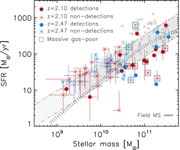
Figure 1. Distribution of our targets in the SFR–M* plane in comparison with the star-forming main sequence. Sources detected with ALMA are represented by the blue and red solid circles while nondetections are identified with the blue and red asterisks. Blue symbols correspond to those galaxies in the z = 2.47 protocluster while red symbols denote members of the z = 2.10 structure. The adopted control sample drawn from Scoville et al. (2016) is shown as gray asterisks. Additionally, two different parameterizations of the star-forming main sequence at the mean redshift of our sample are shown. The gray shaded area represents the relation derived by Speagle et al. (2014) and gray dashed line the one reported by Schreiber et al. (2015). Our sample spans a large range of SFR and stellar mass, representative of the main sequence population. Interestingly, at high stellar masses, an evolved population of galaxies with low SFRs seems to be manifested. Some of them (identified by the black squares) have indeed very low gas mass fractions (Section 4.2) and red colors (Section 4.3), supporting the environmental quenching scenario discussed in Section 4.3.
Download figure:
Standard image High-resolution imageIn summary, our final sample includes a total of 68 sources within the two structures, 27 in the z = 2.47 overdensity and 41 in the z = 2.10 structure. Although our work focuses on galaxies with M⋆ ≳ 1010 M⊙, we include several members with 109 M⊙ < M⋆ < 1010 M⊙ which lie within the ALMA primary beam (see Tables 1 and 2 and Figure 1). This is one of the largest samples of z ≳ 2 galaxies in dense environments for which gas masses have been derived, comprising sources representative of the "normal" star-forming galaxy population, and hence, ideal to test our understanding of gas fueling in protocluster environments.
This subsample of massive sources has a good analogous control sample, which allows for a direct comparison between the properties of the field and the protocluster galaxies and, consequently, a better understanding of the environmental effects. The adopted field scaling relations come from Scoville et al. (2016), who reported ALMA Band 7 (ν = 345 GHz) observations toward ∼55 targets at the same redshifts ( ), UV-luminosities, and masses (1010 M⊙ ≲ M⋆ < 4 × 10¹¹ M⊙; see Figure 1), yet residing in less dense environments (Darvish et al. 2018). These sources were drawn from the NIR-selected catalogs of Ilbert et al. (2013) and Laigle et al. (2016), similar to those used for the identification of the protocluster galaxies targeted in this work. Additionally, their gas masses were derived employing exactly the same methodology adopted here (see details in Section 3.1), and stellar masses and star formation rates were also estimated following similar procedures (see Section 3.2), allowing us to make a balanced comparison.
Given that the completeness of our sample drops at M⋆ ≲ 1010 M⊙ where, additionally, we lack a control sample, the conclusions from this work focus only on the most massive objects with M⋆ ≳ 1010 M⊙.
2.2. ALMA Observations and Detection of Dust Continuum
ALMA Band 6 observations were conducted on 2017 April 4 as part of the Cycle 4 program 2016.1.00646.S (PI: C. Casey), using the 12 m antennae in a relatively compact configuration (with the longest baselines at 0.46 km). These observations comprise a total of 46 pointings with an average on-source integration time of ∼5 minutes, encompassing a total of 68 spectroscopically confirmed galaxies within the two studied protocluster structures. The correlators were configured to maximize the bandwidth in order to increase the continuum sensitivity, providing a total bandwidth of 7.5 GHz centered at 233 GHz (≈1.3 mm).
Data reduction was individually performed following the ALMA reduction pipeline scripts in CASA (version 4.7.2). A few noisy channels in two different spectral windows were flagged for all the pointings before imaging. The continuum maps were obtained using a natural weighting of the visibilities in order to obtain the highest sensitivity, and using a pixel size of 0 12 (roughly seven times smaller than the beam size), yielding central noises between σ1.3 mm = 40–50 μJy/beam and a typical synthesized beam size of θFWHM ≈ 09.
These continuum images are used to search for dust emission for each individual galaxy within 1'' of their respective optical positions. This search radius accounts for any astrometry offset between the ALMA and the optical images (e.g., Dunlop et al. 2017) and for real misalignments between the dusty regions and the bulk of the stellar emission (e.g., Swinbank et al. 2010; Hodge et al. 2016). To derive the flux densities a simple peak-finding algorithm is implemented on the primary-beam corrected images. A source is considered detected only if it satisfies a detection threshold of ≥3σ, for which less than one spurious detection is expected given our positional priors. In this process, the local noise is computed to be the 68th percentile of the distribution of pixel values, which corresponds to ±1σ for a Gaussian distribution. The errors calculated with this method are consistent with those derived by measuring the standard deviation of small off-source apertures. From all the 68 protocluster galaxies which lie within our surveyed area, 19 sources were detected above our adopted threshold, implying a detection rate of ≈25%–30% in each structure. The derived flux density of the detected targets, and the 3σ upper limits of the nondetections, are reported in Tables 1 and 2 (Appendix B), while Hubble Space Telescope (HST)/ALMA cutouts are shown in Appendix C.
To derive better constraints on the average flux densities of the nondetections, a stacking analysis was performed. We extract small cutouts in the image plane centered at the position of each galaxy and then combine them in a weighted average. Weights are estimated as the squared inverse of the noise measured around each source. Finally, the adopted stacked flux density (or upper limit if <3σ) corresponds to the maximum value within 1'' of the center of the stacked image. This stacking procedure was performed for different subsamples defined by SFR, stellar mass, or redshift, which are reported in Table 3.
3. Derivation of Gas Masses, Stellar Masses, and Star Formation Rates
3.1. ISM Masses
Scoville et al. (2014, 2016) developed the physical and empirical bases for using the long wavelength Rayleigh–Jeans dust emission as a probe of the ISM gas content of galaxies, calibrating a ratio between the specific luminosity at rest-frame 850 μm to the total ISM mass. Our ALMA observations trace the rest-frame ∼410 and 350 μm emission for the z ∼ 2.10 and 2.47 protocluster galaxies, respectively, probing hence the Rayleigh–Jeans regime. Following Scoville et al. (2016) we derive the ISM masses using:
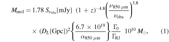
where α850 μm is the empirically calibrated ratio between long-wavelength dust luminosity and molecular gas (i.e.,  ), νobs = 233 GHz is the observed frequency, DL is the luminosity distance at the redshift z, and ΓRJ is the correction for the departure in the rest frame of the Planck function from Rayleigh–Jeans (i.e.,
  ) given by

with  . The uncertainties in the derived masses from this calibration are expected to be less than 25% (Scoville et al. 2016).
ISM masses were calculated for all the ALMA-detected galaxies and their associated errors were obtained by propagating the uncertainties on the flux densities. For those galaxies not detected in continuum emission, 3σ upper limits on the ISM were derived using the flux density upper limits. Additionally, the stacked fluxes described above were also used to derive stacked ISM masses (or upper limits in case of nondetections) for different subsamples divided by SFR or stellar mass. These results are summarized in Tables 1–3 (B).
3.2. Stellar Masses and Star Formation Rates
The large ancillary data available in the COSMOS field provide an exquisite set of photometric measurements in multiple bands for our sample of galaxies, which can be used to estimate stellar masses and star formation rates through spectral energy distribution (SED) modeling. We use the COSMOS2015 catalog (Laigle et al. 2016; the same used by Scoville et al. 2016, from which our control sample is extracted) to obtain the photometry of each of our targets by matching counterparts within a 1'' radius. The catalog includes YJHKs observations from the UltraVISTA survey, Y-band images from the Subaru telescope, infrared photometry from Spitzer, in addition to other data spanning from Galaxy Evolution Explorer near-ultraviolet to SPIRE/Herschel far-infrared, comprising more than 30 bands.
We perform our own SED fitting using all the available photometry, including our new ALMA data, using the MAGPHYS code (da Cunha et al. 2008, 2015), which adopts an energy balance technique between the stellar and dust emission. This approach implies that the stellar component is coupled to the dust-emitting region. While this does not necessarily apply for extreme DSFGs (e.g., Hodge et al. 2016), it usually does for less extreme star-forming galaxies like those studied in this work. The fitting was done with a fixed redshift according to the spectroscopic redshift of each source, using the spectral population synthesis models of Bruzual & Charlot (2003), with a Chabrier (2003) IMF, and a continuous delayed exponential star formation history, similar to the parameters adopted in the work by Laigle et al. (2016). The stellar masses derived for the galaxies presented here are in good agreement with those reported in the COSMOS2015 catalog with a mean ratio of  . All the estimated SFRs and M⋆ are also reported in Tables 1 and 2 and shown in Figure 1.
4. Results
4.1. The Star Formation Efficiency
The star formation efficiency, typically measured as the SFR per unit gas mass ( ), is an important quantity in the understanding of the star formation activity and stellar mass growth, which is directly linked to the gas depletion timescale (
 ). Testing its universality or dependence on other parameters, such as stellar mass, redshift, or environment, is required in order to have a complete view of the structure formation in the universe. Our observations and the measurements of the molecular gas content and SFR described above (see Section 3) allow us to study the SFE in one of the largest and most complete samples of protocluster galaxies at z > 2, shedding light on the influence of the environment on this quantity.
In Figure 2 we explore the SFE of these protocluster galaxies via the SFR–Mmol plane. Thirteen out of the 18 detected galaxies shown in this plot (∼70%) lie, within the error bars, on the field scaling relation. To quantitatively compare the SFEs of the protocluster galaxies with those of our control sample, we perform a Kolmogorov–Smirnov test between the two distributions, from which we derive a probability of p = 0.81 that both of them are drawn from the same parent distribution (when including only those detected galaxies with  , if we include all the detections the probability is p = 0.27).
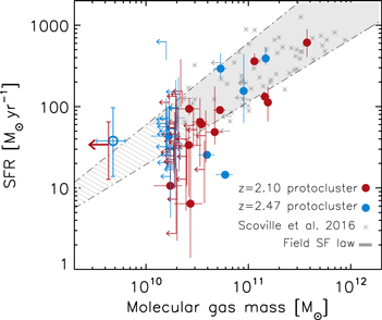
Figure 2. SFR–Mmol relation as a proxy for the SFE. The z = 2.10 and 2.47 protoclusters' member galaxies detected by ALMA are represented by the red and blue filled circles, respectively, while the individual nondetections are plotted as 3σ upper limits (small red and blue left arrows). The 3.3σ detection from the stacking of the nondetected galaxies with  in the z = 2.47 protocluster is illustrated by the large open blue circle, while the 3σ upper limit derived from the stacking of the analogous galaxies in the z = 2.10 protocluster is illustrated by the large red left arrow. Most of our detections and upper limits are consistent with the star formation law found for field galaxies at similar redshifts, represented by the gray shaded area and individual gray asterisks (Scoville et al. 2016). Those sources lying below the relation and those whose upper limits lie above it are discussed in the main text.
Download figure:
Standard image High-resolution imageAt the probed evolutionary stage of these protoclusters, the SFEs of the most massive galaxies show consistent values to those expected for coeval field galaxies. Although a nonnegligible fraction of the detected galaxies seems to lie below the field relation while some upper limits suggest galaxies lying above it. From the four detected sources that lie significantly below the field relation (or to the right of it), two are part of the z = 2.10 protocluster and two are from the z = 2.47 structure. The two sources from the z = 2.47 protocluster also lie below the star-forming main sequence (Figure 1), which implies that their low SFE is driven by the reduced SFR rather than by an excess of molecular gas. Indeed, these sources lie on the expected relation if their offset from the main sequence is taken into account, as shown in Appendix A. The two sources from the z = 2.10 structure show SFRs in agreement with main-sequence galaxies and their high SFEs seem to be caused by their enhanced molecular gas masses (see Appendix A). Interestingly, most of the results derived from the stacking of the nondetections, which probe—on average—galaxies with M* ∼ 1 × 10¹⁰  (see Table 3), seem also to be in agreement with the extrapolation of the field scaling relation with a few sources lying above it (see Appendix A).
Heterogeneous results regarding the SFEs of protocluster galaxies have been presented in the literature, including some in agreement with our results. For example, Lee et al. (2017) detected CO(3 − 2) line emission in seven star-forming galaxies associated with the protocluster 4C23.56 at z = 2.49 and derived a median SFE consistent with the reference sample (although different results have been reported in the same structure, as discussed below; Tadaki et al. 2019). Dannerbauer et al. (2017) detected an extended CO(1 − 0) emitting disk in a protocluster member galaxy at z ≈ 2.15, whose gas properties and SFR follow the same relation as normal field galaxies. Similarly, Darvish et al. (2018) used ALMA dust continuum observations to investigate the role of environmental density on the molecular gas content in a large sample of ∼400 massive (M⋆ ≳ 1010 M⊙) galaxies within z ≈ 0.5–3.5, where the density was estimated by the projected surface density of galaxies over different redshift slices, and concluded that the SFE is independent of galaxy overdensity. Wang et al. (2018) obtained CO(1 − 0) observations toward a concentrated group of 14 galaxies at z ≈ 2.51 which might be associated with the z ≈ 2.47 protocluster structure presented here (see also Cucciati et al. 2018; J. B. Champagne et al. 2019, in preparation). Their estimated SFEs show a large variety of values, although an interesting tentative trend suggests a high SFE toward the center of the small surveyed core. Gómez-Guijarro et al. (2019) reanalyzed the Wang et al. sample with deeper observations and present new CO observations in two new protoclusters at z = 2.13 and 2.60, finding rather similar SFEs to the field. Additionally, studies of more evolved (collapsed) clusters at z ∼ 1.6–2.1 targeting CO emission lines have found similar SFEs or depletion timescales (τ = 1/SFE) to the ones measured in field galaxies at similar redshifts (Rudnick et al. 2017).
On the other hand, Tadaki et al. (2019) presented CO(3 − 2) observations toward 66 Hα-selected galaxies in three protoclusters at z = 2.16, 2.49, and 2.53. Interestingly, in the stellar mass range of  they reported SFEs lower (i.e., longer depletion timescales) than expected from the scaling relation, although these galaxies only represent 30% of all the sources within this stellar mass range. The rest of the galaxies (including all those with
  ) are in agreement with the field relations. In line with these results, Noble et al. (2017) found depletion timescales systematically higher than the scaling relation for nine CO(3 − 2)-detected galaxies in a cluster at z ∼ 1.6, although most are within one standard deviation of the relation (plus several nondetections whose upper limits are in agreement with the field). Similarly, Hayashi et al. (2018) presented CO(3 − 2) observations in several cluster galaxies at z ∼ 1.5 finding again systematically longer depletion timescales, although ∼50% of their sample might be in agreement the expected relation for the field (when nondetections are taken into account).
Although our results suggest that most of the massive ( ) galaxies have SFEs similar to coeval field galaxies, it is clear that other works in the literature have revealed (proto)cluster galaxies with a large variety of properties, with some of them having SFEs similar to coeval field galaxies and others lying off the expected relations. Larger samples of high-redshift clusters and protoclusters, as well as deeper observations to mitigate nondetections, are hence required to fully understand the star formation activity and gas fueling in these overdense structures.
4.2. Gas Content and Gas Fraction
Figure 3 shows the combined gas mass function of the two protoclusters, which is formally a lower limit given the incompleteness of our follow-up survey (only a fraction of the known protocluster members were observed; see Section 2.1) and the possible existence of more unidentified member galaxies. This estimation assumes a volume of 15,000 cMpc3 for each structure, as estimated by Casey (2016). Note that this volume encompasses the z ≈ 2.47 overdensity studied here, but not the larger structure reported in the literature with a redshift range of z = 2.42–2.51 (Cucciati et al. 2018; although the volume would only increase by a factor of ∼2). The first bin of our gas mass function comes from the stacked detection of 20 galaxies (14 in the z = 2.10 structure and 6 in the 2.47; see Table 3), while the rest come directly from the individual detections.
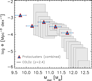
Figure 3. Comparison between the COLDz gas mass function derived from  observations at z ≈ 2.4 (gray squares, Riechers et al. 2019) and the gas mass function derived from our ALMA follow-up of protocluster galaxies at similar redshifts (colored triangles). As described in the text, our measurements are formally lower limits since only a fraction of the protocluster members were observed. Therefore, it is likely that, after taken into account the incompleteness effects, the protoclusters show an enhanced gas mass function (and hence gas volume density) compared to the field.
Download figure:
Standard image High-resolution imageThe derived lower limit of the protoclusters' gas mass function is of the same order of magnitude as the field gas mass function at these redshifts,12 as shown in Figure 3). Therefore, it is likely that these protoclusters have an enhanced gas mass function or a higher gas volume density than the one measured in the field, after taking into account all the incompleteness described above. Indeed, enhanced gas volume densities have been measured for other similar overdense structures (e.g., Lee et al. 2017).
In Figure 4 we plot the derived gas mass fraction,  , as a function of stellar mass for the protocluster galaxies, and other samples taken from the literature, including our reference sample. As can be seen, most of the ALMA-detected galaxies, represented by the blue and red filled circles in the figure, show gas fractions that resemble those estimated for coeval field galaxies and their scaling relations,13
which is illustrated by the gray shaded region (see also Appendix A). The individual upper limits derived from the ALMA nondetections for those galaxies with M⋆ ≲ 5 × 10¹⁰ M⊙ are also consistent with the field relation, but those of the most massive galaxies point toward reduced gas fractions when compared to the field (see also Appendix A).
, as a function of stellar mass for the protocluster galaxies, and other samples taken from the literature, including our reference sample. As can be seen, most of the ALMA-detected galaxies, represented by the blue and red filled circles in the figure, show gas fractions that resemble those estimated for coeval field galaxies and their scaling relations,13
which is illustrated by the gray shaded region (see also Appendix A). The individual upper limits derived from the ALMA nondetections for those galaxies with M⋆ ≲ 5 × 10¹⁰ M⊙ are also consistent with the field relation, but those of the most massive galaxies point toward reduced gas fractions when compared to the field (see also Appendix A).

Figure 4. Molecular gas fraction of the protocluster members as a function of stellar mass (blue and red for the z = 2.10 and 2.47 structures, respectively), along with other measurements from the literature. Solid circles represent the ALMA-detected galaxies while the small downward arrows are the respective upper limits for the individual nondetections. Large open circles and large downward arrows represent the results from the stacking of the nondetections of subsamples divided by stellar mass and redshift (see Table 3). The typical 3σ detection limit of our survey is illustrated by the dotted line. The derived gas mass fraction of most of the detected galaxies are in good agreement with those measured for field galaxies at similar redshifts and with the field scaling relation (gray shaded region, Scoville et al. 2016), implying that these sources do not show enhanced gas masses. For comparison, results from studies on other protoclusters are also included (gold, gray, and green triangles for Lee et al. 2017; Gómez-Guijarro et al. 2019, and Tadaki et al. 2019, respectively), showing both galaxies with enhanced gas fractions and galaxies in agreement with the field (in addition to several nondetections). Interestingly, in the systems studied in this work, there are several massive nondetected galaxies for which the estimated stacked upper limits on their gas mass lie significantly below the expected field relation (large blue and red downward arrows), resembling those measured for passive quiescent galaxies and suggesting that they are likely transitional galaxies soon-to-be quenched (see discussion in Section 4.3).
Download figure:
Standard image High-resolution imageDifferent works from the literature have also reported gas fractions in protocluster galaxies in agreement with the field. For example, Lee et al. (2017) found that most of the observed galaxies in a z = 2.49 protocluster show gas fractions comparable to those of field galaxies. Their detections are plotted in Figure 4 (gold triangles), where it can be seen that their values are in agreement with our measurements.
Figure 4 also shows the results from Tadaki et al. (2019) and Gómez-Guijarro et al. (2019) who observed galaxies in several overdensities within z = 2.17–2.60. Besides the longer gas depletion timescales found by Tadaki et al. (2019) for some galaxies with  , sources with high gas mass fractions were also found (although they represent ≲50% of all the galaxies within this stellar mass range). Most of the remaining sources, and all the galaxies with M⋆ ≳ 1010 M⊙, have gas fractions (or upper limits) in agreement with the field relation. Similarly, Gómez-Guijarro et al. (2019) found some galaxies with large gas fractions (all of them with M⋆ ≲ 6 × 10¹⁰ M⊙) despite showing SFEs consistent with the field. Nevertheless, most of these gas-rich galaxies lie above the main sequence, and therefore, might be more representative of the starburst population. Galaxies with enhanced gas fractions have also been reported in more evolved (collapsed) clusters at lower redshifts, like those reported by Noble et al. (2017) and Hayashi et al. (2018) at z ∼ 1.5.
While some protoclusters show most of their members with gas fractions in agreement with coeval field galaxies, as those presented in this work (see also Lee et al. 2017), there is clear evidence that other structures have individual systems with large gas masses (e.g., Gómez-Guijarro et al. 2019; Tadaki et al. 2019), as discussed above. Discriminating between if these gas-rich systems exist preferentially in overdense environments or if they represent only outliers of the general population (note that this kind of outlier also exists in the field) requires deeper observations of complete samples, even deeper than the ones presented here. For example, the results of Noble et al. (2017), who present one of the best lines of evidence for the existence of sources with enhanced gas masses, are based on the detection of only seven individual sources from a parent sample of 49 cluster members. Similarly, the gas-rich galaxies found by Hayashi et al. (2018) come from 18 detections out of a parent sample of 65 sources. Although cluster-to-cluster variations, reflecting different evolutionary stages (e.g., Shimakawa et al. 2018; Gómez-Guijarro et al. 2019) are expected, it is still unclear if the bulk of the population in the aforementioned cluster also have enhanced gas fractions. Unfortunately, deeper ALMA spectroscopic observations would require several hours of on-source time per target, making spectroscopic observations of larger samples prohibitive. Continuum observations as a proxy for gas masses (Scoville et al. 2016) will therefore play a determinant role in our understanding of the star formation activity during the early phases of cluster assembly.
4.3. Environmental Quenching
As shown in Figure 4, some of the most massive galaxies studied in this work show very low gas mass fractions, fgas ≲ 6%–10% (see also Wang et al. 2018), resembling those estimated for quiescent galaxies (note, however, that most of the constraints on the gas fraction of passive galaxies are limited to z < 2; e.g., Sargent et al. 2015; Gobat et al. 2018; Spilker et al. 2018; Bezanson et al. 2019). These massive gas-poor galaxies might be in a transitional phase toward a quiescent mode, and hence, they are ideal sources to study the quenching mechanisms, especially the effects of environmental quenching.
In Figure 1 we highlight the most massive gas-poor systems ( ) with black squares. As can be seen, most of them (seven out of nine) lie below the star-forming main sequence, supporting a possible quenching phase. The galaxy that lies above the main sequence is known to host an AGN (based on an X-ray detection; Laigle et al. 2016), and therefore it is likely that its SFR might be overestimated (note that only six of the whole sample are classified as AGN, as mentioned below).
To further explore their possible passive nature, Figure 5 shows the rest-frame U − V color of our sample of protocluster galaxies, which has been proven to be a good indicator to disentangle the quiescent and star-forming populations of galaxies via blue and red populations (e.g., Bell et al. 2004; Brown et al. 2007; Faber et al. 2007). This figure clearly shows that the most massive galaxies undetected by ALMA have red colors, as would be expected if they are in the quenching process.
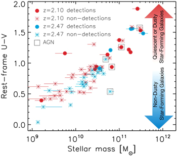
Figure 5. Rest-frame U − V color-stellar mass relation. Galaxies detected with ALMA are represented by the filled blue and red solid circles (for those in the z = 2.47 and 2.10 protoclusters, respectively), while the asterisks represents the nondetections. The most massive galaxies show redder colors than the less massive and include both dusty star-forming sources and quiescent evolved gas-poor systems. Those galaxies hosting an AGN -identified via X-ray detection- are indicated with a black open square.
Download figure:
Standard image High-resolution imageIn Figure 6 we show instead the rest-frame (U − V) versus (V − J) color–color diagram. This UVJ plot is commonly used to distinguish between dusty, star-forming galaxies and quenched galaxies since both populations usually have red colors (e.g., Wuyts et al. 2007; Williams et al. 2009). While it is true that the massive gas-poor galaxies described above are not entirely within the quiescent parameter space, they lie very close to it. Additionally, it as been shown that some passive galaxies remain outside of the UVJ selection area well after their actual quenching (up to almost 0.5 Gyr), particularly, for those in which the SFR decreases abruptly, called post-starburst galaxies (Merlin et al. 2018; Belli et al. 2019). To illustrate this, we plot in Figure 6 the expected path on the UVJ diagram of a galaxy with a fast quenching process described by a tau model with a short timescale of τ = 100 Myr (see details in Belli et al. 2019). The colors predicted by this scenario (see also Merlin et al. 2018 for similar results) are in agreement with those measured for some of the massive gas-poor galaxies in our sample. The well-studied post-starburst galaxy at z ≈ 3 reported by Marsan et al. (2015), has, actually, very similar colors (see Figure 6).
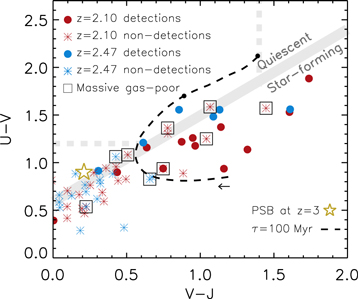
Figure 6. Rest-frame U − V vs. V − J color–color diagram (not corrected for dust attenuation). Protocluster galaxies within the z = 2.41 structure are represented by the blue symbols while those in the z = 2.10 are shown in red. Solid circles represent ALMA-detections while asterisks indicate nondetections. The cut proposed by Belli et al. (2019) to separate star-forming and quiescent galaxies is indicated by the gray diagonal solid line (dashed lines indicate additional constraints, e.g., Muzzin et al. 2013). The most massive ( ) gas-poor galaxies in our sample (illustrated with black squares) are thought to be post-starburst or transition galaxies (see the discussion in Section 4.3). As a reference, a well-studied post-starburst galaxy at z ≈ 3 (Marsan et al. 2015) is plotted as a gold star as well as the predicted color evolution for a fast quenching path described by a tau model with a short timescale of τ = 100 Myr (Belli et al. 2019).
Download figure:
Standard image High-resolution imageThese findings, combined with the ALMA nondetections, suggest that the massive gas-poor sources shown in Figure 4 are evolved galaxies, most likely post-starburst or in transition to a quiescent mode.
Is the evolution of these high-mass gas-poor transition galaxies driven by the overdense protocluster environment? Quiescent massive galaxies have been found in the field up to z ≳ 3 (e.g., Straatman et al. 2014; Glazebrook et al. 2017), and therefore a comparison between the field and these protocluster galaxies is necessary to understand the impact of the environment on the quenching process. In Figure 7, we compare the ALMA continuum detection fraction of our protocluster galaxies to the one derived for our control sample (Scoville et al. 2016) and also to those found in blind blank-field observations (Bouwens et al. 2016; Dunlop et al. 2017), limiting these samples to galaxies within z ≈ 2–3. Note that all the observations have similar depths,14 making the comparison appropriate.
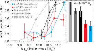
Figure 7. ALMA dust continuum detection fraction as a function of stellar mass for galaxies within z ≈ 2–3. Previous ALMA blank-field observations (Bouwens et al. 2016; Dunlop et al. 2017) and follow-ups of field galaxies (Scoville et al. 2016) show a higher detection fraction than the one achieved toward the protocluster galaxies studied here (colored in red and blue), despite having similar depths. The difference is clearly evidenced by the detection fraction of the most massive galaxies (M⋆ > 2 × 10¹⁰ M⊙), as shown in the right panel. This implies a higher fraction of quenched gas-poor galaxies in the protocluster structures than the one found in the field at the same cosmic epoch, suggesting that massive galaxies in dense environments undergo an accelerated evolution.
Download figure:
Standard image High-resolution imageInterestingly, the observations toward protocluster member galaxies show a lower detection fraction than those for the field samples, particularly for the high-mass galaxies (Figure 7). This is also true even if we only compare our results to those from the blind blank-field surveys, which have no biases due to selection effects. This difference is found in both the z = 2.10 and the z = 2.47 protocluster structures. These results imply that the most massive galaxies in protocluster environments experience an accelerated evolution compared to the field sources, given the higher fraction of quiescent gas-poor galaxies.
We also estimate an average environmental quenching efficiency, defined as  , which represents the fraction of field galaxies required to be quenched in order to match the observed quenching fraction in the protoclusters. For the two structures studied here, we estimate an average quenching efficiency of
  . This quenching efficiency is indeed in agreement with those found for more evolved clusters at z ≈ 1.0−1.6 (see the compilation by Nantais et al. 2016). All these results suggest that we are witnessing the first stages of the well-known environmental quenching found in lower redshift and/or more evolved clusters (e.g., Tran et al. 2009; Alberts et al. 2014; Newman et al. 2014; Nantais et al. 2016; Lee-Brown et al. 2017; Ji et al. 2018; Noirot et al. 2018; Paulino-Afonso et al. 2018; Shimakawa et al. 2018), which originates the excess of red sources in local galaxy clusters (Dressler 1984).
Understanding the mechanisms that drive this evolution requires further observations than are included here. However, it is clear that these mechanisms should involve gas consumption or removal, or at least a halting of gas accretion, given the small gas fractions derived for these red galaxies (see also Man et al. 2019). Note that counterexamples to this exist, i.e., passive galaxies with significant gas reservoirs (e.g., Rowlands et al. 2015; Suess et al. 2017; Gobat et al. 2018), although in a variety of galaxy environments from isolated systems to small groups. Some of the typically cited quenching processes in high-density environments are AGN feedback (e.g., Kauffmann et al. 2003; Fabian 2012; Shimakawa et al. 2018), major and minor mergers (e.g., Davis et al. 2019; Maltby et al. 2018), ram pressure stripping (meaning gas being removed from the galaxies by the IGM, e.g., Gunn & Gott 1972; Larson et al. 1980; Boselli & Gavazzi 2006; Foltz et al. 2018, although see Dannerbauer et al. 2017), and starvation (when gas accretion is stopped).
In Figure 5, we identify those galaxies that are likely to host an AGN based on their detection with Chandra X-ray Observatory (using the match reported by Laigle et al. 2016 to the Chandra COSMOS catalogs by Civano et al. 2016; Marchesi et al. 2016). Only a few galaxies are X-ray detected (all of them have M⋆ ≳ 3 × 10¹⁰ M⊙; see Tables 1 and 2), and there is not a clear trend between AGN activity and quenching since some of them are detected by ALMA while others are not. Nevertheless, we cannot rule out this mechanism as the main quenching processes given the incompleteness related to the AGN identification.
To shed light on other quenching mechanisms possibly involved, we estimate an upper limit on the quenching timescale adopting the average mass-weighted stellar age of the massive gas-poor galaxies derived from the SED fitting (see Section 3.2). Given that this quantity is related to the time since the onset of star formation,15
any quenching mechanism must have a shorter timescale. To be conservative, we adopt the longest age from the 97.5th percentile of the stellar age distribution, resulting in an upper limit on quenching timescale of  . Similar timescales have been reported for passive galaxies in lower redshift clusters (e.g., Muzzin et al. 2014; Davis et al. 2019; Socolovsky et al. 2018) and are usually associated with ram pressure stripping and/or mergers (e.g., Steinhauser et al. 2016). In line with these findings, Casey et al. (2015) and Hung et al. (2016) found slightly higher fractions of irregular and interacting galaxies in the z = 2.47 and 2.10 structures than in their control samples (although with a low statistical significance of ∼1.5σ), supporting the influence of galaxy mergers in the evolution of galaxies in overdense environments.
Given that the protocluster structures studied here are still in an assembly phase, these results indicate galaxy preprocessing, meaning the interactions between groups of galaxies prior to the settling in a cluster potential, might be also an important quenching mechanism (see also Zabludoff et al. 1996; Haines et al. 2015; Bianconi et al. 2018; Olave-Rojas et al. 2018).
Alternatively, the advanced evolutionary stage of some massive protocluster member galaxies can be explained by an earlier onset of the star formation activity (e.g., Steidel et al. 2005). Nevertheless, the mean stellar age of the red, massive gas-poor galaxies is consistent with the ages derived for the ALMA-detected galaxies (when using the same stellar mass threshold). Similarly, the stellar ages derived for the Scoville et al. (2016) sample, representative of the average field population, show values in agreement with the protocluster galaxies studied here. Although we cannot rule out specific sources with premature star formation, we conclude that environmental effects, as those discussed above, most likely nurture an accelerated evolution in these systems.
5. Conclusions
We have presented the largest census of molecular gas mass in protocluster member galaxies at z ≳ 2, which combined with multiwavelength observations and SED modeling, allowed us to characterize the gas mass fraction and star formation efficiency for these sources, and to inquire into the environmental quenching during the earliest phases of cluster assembly.
ALMA Band 6 (ν = 233 GHz) observations were obtained for a total of 68 spectroscopically confirmed galaxies within two large and massive overlapping protoclusters in the COSMOS field at z = 2.10 and 2.47, respectively, comprising most of the known massive galaxies with  in these structures, plus other less massive (
 ) galaxies that lie within the field of view. Given the low completeness level for the low-mass galaxies, our conclusions regard only to the most massive systems (
 ).
).
ISM masses were derived from the Rayleigh–Jeans dust continuum emission probed by the ALMA data, following the methodology developed by Scoville et al. (2014, 2016), while SFRs and stellar masses were estimated by fitting the photometric SED using MAGPHYS (da Cunha et al. 2008, 2015) and the rich multiwavelength photometry compiled by Laigle et al. (2016) (see Section 3). All the derived properties are reported in Tables 1–3.
Our analysis showed that, at the probed evolutionary stage of these systems, the star formation efficiency of most of the protocluster members are similar to those found for coeval field galaxies and are in agreement with the field scaling relations (see Figure 2), although, a nonnegligible fraction of the less massive systems might have enhanced efficiencies. Most of these protocluster galaxies have also gas fractions that resemble those estimated for coeval field galaxies (Figure 4), with the exception of a few of the most massive systems showing very low gas masses.
The effects of the environment are more evident when looking at the fraction of quenched galaxies. The larger number of massive gas-poor galaxies (ALMA nondetections) in the protoclusters in comparison to the field (Figures 4 and 7) suggests that these protocluster galaxies are undergoing an accelerated evolution (see also Hayashi et al. 2018; Shimakawa et al. 2018; Wang et al. 2018). These massive gas-poor systems have low gas mass fractions of fgas ≲ 6%–10% (Figure 4) and red colors (Figures 5 and 6) which are in agreement with those found for post-starburst and quiescent galaxies at lower redshifts (e.g., Sargent et al. 2015; Belli et al. 2019; Gobat et al. 2018).
Environmental quenching is therefore manifested during the early phases of cluster assembly and must involve rapid mechanisms (on a timescale of hundreds of megayears). From our observations, we derive an upper limit on the quenching timescale of τq < 1 Gyr and a quenching efficiency of  . Note that these estimations concern only galaxies with
  which are considered passive given their low gas content and red colors (see details in Section 4.3). Some of the processes typically cited in the literature with such timescales include AGN feedback, ram pressure stripping, and galaxy mergers. Regardless of their relative importance, it is clear that these mechanisms should involve gas consumption or removal, or at least to halt gas accretion, given the small gas fractions derived for these red galaxies, nevertheless, further observations than those analyzed here are required to draw further conclusions.
Given that the protoclusters studied here have not yet collapsed, our results suggest that quenching before virialization, also known in the literature as galaxy preprocessing, is an important mechanism related to the environmental quenching.
We thank Anthony Remijan and Jeremy Thorley from the North American ALMA Science Center (NAASC) for their help with data reduction and retrieval. J.A.Z. and C.M.C. thank the University of Texas at Austin College of Natural Sciences for support, in addition to NSF grant AST-1714528 and AST-1814034. E.T. acknowledges support from FONDECYT Regular 1160999, CONICYT PIA ACT172033 and Basal-CATA PFB-06/2007 and AFB170002 grants. H.D. acknowledges financial support from the Spanish Ministry of Science, Innovation and Universities (MICIU) under the 2014 Ramón y Cajal program RYC-2014-15686 and AYA2017-84061-P, the latter one cofinanced by FEDER (European Regional Development Funds). S.T. acknowledges support from the European Research Council (ERC) Consolidator Grant funding scheme (project ConTExt, grant No. 648179). The Cosmic Dawn Center is funded by the Danish National Research Foundation.
This paper makes use of the following ALMA data: ADS/JAO.ALMA#2016.1.00646.S. ALMA is a partnership of ESO (representing its member states), NSF (USA) and NINS (Japan), together with NRC (Canada) and NSC and ASIAA (Taiwan) and KASI (Republic of Korea), in cooperation with the Republic of Chile. The Joint ALMA Observatory is operated by ESO, AUI/NRAO, and NAOJ.
Appendix A: Comparison to Other Scaling Relations
The main results of this paper remain if we instead adopt the scaling relations derived by Tacconi et al. (2018), which take into account stellar masses and SFRs simultaneously. Figure 8 shows the SFE as a function of offset from the main sequence ( , left panel) for the protocluster and field galaxies. Almost 80% of the detected sources (14 out of 18) lie on the Tacconi et al. scaling relation. Interestingly, there is a nonnegligible fraction of galaxies whose lower limits on the SFEs place them above the field relation. However, most of these sources have stellar masses below
  , probing a stellar mass range that suffers from low completeness in our sample, which prevents us from investigating the relevance of these galaxies in comparison to the bulk of the population. As mentioned above, the conclusions from this work focus only on the most massive objects with
  . On the other hand, most of the gas fractions of the protocluster member galaxies (right panel) lie on or below the field relation. These results suggest that protocluster galaxies undergo an accelerated evolution, which produces an enhanced fraction of passive gas-poor galaxies than relative to the field.
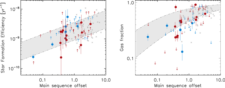
Figure 8. Left: distribution of SFEs (SFR/Mgas; left:) and gas fractions (right) as a function of main-sequence offset (SFR/SFRMS) for the protocluster member galaxies studied in this work. Those galaxies in the z = 2.47 overdensity detected by ALMA are represented by the blue solid circles while nondetections are illustrated by the blue asterisks. Those in the z = 2.10 are shown with red symbols (solid circles and asterisks for the detections and nondetections, respectively). Gray asterisks correspond the control sample adopted in our study (Scoville et al. 2016). The gray shaded area represents the Tacconi et al. (2018) field scaling relations for main-sequence galaxies at a redshift and stellar mass representative of our sample with ±0.3 dex scatter.
Download figure:
Standard image High-resolution imageAppendix B: Derived Properties
The derived properties for the galaxies studied in this work, including 1.3mm flux densities, stellar and gas masses, and SFRs, are reported in Tables 1–3.
Table 1. Properties of the z = 2.10 Protocluster Galaxies Observed with ALMA
| ID | zspec | SNR | S1.3 mm | M⋆a | SFRa | MISMb |
|---|---|---|---|---|---|---|
| (μJy) | (×1010 M⊙) | ( ) ) |
(×1010 M⊙) | |||
| J100031.84+021242.7 | 2.1043 | 51 | 2301 ± 45 |

|

|
37.3 ± 0.7 |
| J100041.25+021426.5 | 2.0880 | 21.8 | 954 ± 43 |

|

|
15.5 ± 0.7 |
| J100032.73+021331.1c | 2.0908 | 16.4 | 704 ± 42 |

|

|
11.4 ± 0.6 |
| J100018.24+021242.5 | 2.1021 | 8.9 | 892 ± 100 |

|

|
14.4 ± 1.6 |
| J100042.65+020850.9 | 2.0988 | 7.2 | 324 ± 45 |

|

|
5.2 ± 0.7 |
| J100046.65+021623.9 | 2.0981 | 6.0 | 208 ± 34 |

|

|
3.3 ± 0.5 |
| J095936.45+021614.5c | 2.0903 | 5.4 | 214 ± 39 |

|

|
3.4 ± 0.6 |
| J100016.01+021527.8 | 2.1019 | 5.2 | 289 ± 55 |

|

|
4.6 ± 0.8 |
| J100000.91+020902.6 | 2.0986 | 4.0 | 162 ± 41 |

|

|
2.6 ± 0.6 |
| J100015.02+021538.9 | 2.0922 | 3.2 | 167 ± 51 |

|

|
2.7 ± 0.8 |
| J100022.64+021434.6 | 2.0979 | 3.2 | 106 ± 32 |

|

|
1.7 ± 0.5 |
| J100018.06+021409.9 | 2.0951 | 3.1 | 161 ± 51 |

|

|
2.6 ± 0.8 |
| J100018.55+021817.2 | 2.0924 |

|

|

|

|

|
| J095949.58+022445.3 | 2.0850 |

|

|

|

|

|
| J100018.60+021257.7 | 2.0859 |

|

|

|

|

|
| J100040.82+021822.9 | 2.1001 |

|

|

|

|

|
| J100022.73+021423.6 | 2.1027 |

|
<194 |

|

|
<3.1 |
| J100015.74+021539.6 | 2.1040 | <3.0 | <114 |

|

|
<1.8 |
| J100023.69+021604.1 | 2.0920 | <3.0 | <121 |

|

|
<1.9 |
| J100028.14+021325.9 | 2.0857 | <3.0 | <117 |

|

|
<1.9 |
| J100022.53+021556.3 | 2.0978 | <3.0 | <229 |

|

|
<3.7 |
| J100015.56+022029.6 | 2.0900 | <3.0 | <126 |

|

|
<2.0 |
| J100029.98+021413.1 | 2.0985 | <3.0 | <109 |

|

|
<1.7 |
| J100023.02+021434.4 | 2.0961 | <3.0 | <116 |

|

|
<1.8 |
| J100022.33+021441.7 | 2.0986 | <3.0 | <154 |

|

|
<2.5 |
| J100025.04+021005.9 | 2.0962 | <3.0 | <103 |

|

|
<1.6 |
| J100023.61+021557.3 | 2.0893 | <3.0 | <152 |

|

|
<2.4 |
| J100017.90+021807.1c | 2.0937 | <3.0 | <134 |

|

|
<2.1 |
| J100022.99+021605.2 | 2.0943 | <3.0 | <124 |

|

|
<2.0 |
| J100044.05+021522.2 | 2.0914 | <3.0 | <119 |

|

|
<1.9 |
| J100022.19+021306.3 | 2.0978 | <3.0 | <121 |

|

|
<1.9 |
| J095955.88+022459.0 | 2.0899 | <3.0 | <115 |

|

|
<1.8 |
| J100019.19+021406.5 | 2.1014 | <3.0 | <127 |

|

|
<2.0 |
| J100015.89+021543.7 | 2.1090 | <3.0 | <129 |

|

|

|
| J100015.89+021547.2 | 2.0976 | <3.0 | <151 |

|

|

|
| J095950.32+022206.0 | 2.0902 |

|

|

|

|
<1.9 |
| J100046.37+021622.0 | 2.0891 | <3.0 | <118 |

|

|
<1.9 |
| J100023.30+021612.6 | 2.0950 | <3.0 | <161 |

|

|
<2.6 |
| J100023.38+021606.3 | 2.0917 | <3.0 | <122 |

|

|
<1.9 |
| J100018.53+021306.9 | 2.1056 | <3.0 |

|

|

|
<2.9 |
| J100022.86+021432.3 | 2.0973 | <3.0 | <107 |

|

|
<1.7 |
Notes.
aThe SFRs and stellar masses were derived through an SED-fitting precedure (see Section 3.2). bISM masses were estimated from dust-continuum emission (see Section 3.1). cX-ray detected sources. All the reported upper limits are 3σ values.Download table as: ASCIITypeset image
Table 2. Properties of the z = 2.47 Protocluster Galaxies Observed with ALMA
| ID | zspec | SNR | S1.3 mm | M⋆a | SFRa | MISMb |
|---|---|---|---|---|---|---|
| (μJy) | (×1010 M⊙) | ( ) ) |
(×1010 M⊙) | |||
| J100056.95+022017.2 | 2.4940 | 44.7 | 2095 ± 47 | ⋯ | ⋯ | 32.3 ± 0.7 |
| J100057.56+022011.1 | 2.5130 | 11.3 | 957 ± 84 |

|

|
14.7 ± 1.3 |
| J100057.26+022012.4 | 2.5040 | 10.0 | 583 ± 58 |

|

|
8.9 ± 0.8 |
| J100056.85+022008.8 | 2.5030 | 6.9 | 347 ± 51 |

|

|
5.3 ± 0.7 |
| J100115.18+022349.7 | 2.4710 | 5.5 | 254 ± 46 |

|

|
3.9 ± 0.7 |
| J100057.38+022010.5 | 2.5080 | 5.2 | 384 ± 74 |

|

|
5.9 ± 1.1 |
| J100025.28+022643.3 | 2.4750 | 3.1 | 108 ± 35 |

|

|
1.6 ± 0.5 |
| J100111.03+022043.3 | 2.4670 |

|

|

|

|
<1.6 |
| J100039.40+022155.4 | 2.4571 | <3.0 | <101 |

|

|
<1.5 |
| J100020.50+022421.4 | 2.4720 | <3.0 | <101 |

|

|
<1.5 |
| J100031.13+023103.3 | 2.4680 | <3.0 | <124 |

|

|
<1.9 |
| J100015.38+022448.2 | 2.4740 | <3.0 | <104 |

|

|
<1.6 |
| J100025.09+022500.3 | 2.4709 | <3.0 | <110 |

|

|
<1.6 |
| J100013.61+022604.8 | 2.4630 | <3.0 | <102 |

|

|
<1.5 |
| J100015.86+021939.5 | 2.4750 | <3.0 | <127 |

|

|
<1.9 |
| J100059.45+021957.4c | 2.4710 | <3.0 | <127 |

|

|
<1.9 |
| J100012.36+023707.5 | 2.4750 | <3.0 | <134 |

|

|
<2.0 |
| J100024.21+022741.3 | 2.4790 | <3.0 | <104 |

|

|
<1.6 |
| J100008.88+023044.0 | 2.4750 | <3.0 | <140 |

|

|
<2.1 |
| J100027.12+023253.8 | 2.4745 | <3.0 |

|

|

|
<1.8 |
| J100033.19+022225.0 | 2.4740 | <3.0 | <112 |

|

|
<1.7 |
| J100109.29+022221.5 | 2.4730 | <3.0 | <124 |

|

|
<1.9 |
| J100018.03+021808.5 | 2.4720 | <3.0 | <134 |

|

|
<2.0 |
| J100050.73+021922.4 | 2.4660 | <3.0 | <109 |

|

|
<1.6 |
| J100014.23+022516.7 | 2.4710 | <3.0 | <127 |

|

|
<1.9 |
| J100054.06+022104.3c | 2.4780 | <3.0 | <112 |

|

|
<1.7 |
| J100021.97+022356.5c | 2.4730 | <3.0 | <102 |

|

|
<1.5 |
Notes.
aThe SFRs and stellar masses were derived through an SED-fitting precedure (see Section 3.2). bISM masses were estimated from dust-continuum emission (see Section 3.1). cX-ray detected sources. All the reported upper limits are 3σ values.Download table as: ASCIITypeset image
Table 3. Properties of the Stacked Subsamples
| Subsample | N |

|
 a
a
|
 a
a
|
 b
b
|
|---|---|---|---|---|---|
| (M⊙) | ( ) ) |
(M⊙) | |||
Galaxies with  in the z = 2.10 protocluster in the z = 2.10 protocluster |
11 | 2.0959 |

|

|
<7.6 × 10⁹ |
Galaxies with  in the z = 2.10 protocluster in the z = 2.10 protocluster |
14 | 2.0950 |

|

|
9.0 ± 1.9 × 10⁹ |
Galaxies with  in the z = 2.10 protocluster in the z = 2.10 protocluster |
4 | 2.0931 |

|

|

|
Galaxies with  in the z = 2.47 protocluster in the z = 2.47 protocluster |
6 | 2.4694 |

|

|
8.2 ± 2.5 × 10⁹ |
Galaxies with  in the z = 2.47 protocluster in the z = 2.47 protocluster |
14 | 2.4723 |

|

|

|
Galaxies with  in the z = 2.10 protocluster in the z = 2.10 protocluster |
18 | 2.0957 |

|

|
<4.3 × 10⁹ |
Galaxies with  in the z = 2.47 protocluster in the z = 2.47 protocluster |
23 | 2.4711 |

|

|
4.8 ± 1.4 × 10⁹ |
Notes.
aThe quoted uncertainties on the SFRs and stellar masses actually represent the width of the bins. bThe stacked ISM masses were estimated from the upper limits on the dust continuum using an inverse variance weighting. All the reported upper limits are 3σ values.Download table as: ASCIITypeset image
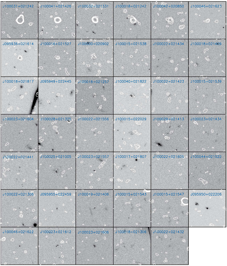
Figure 9. 10'' × 10'' postage stamps in the HST/ACS I-band for all the targets in the z = 2.10 protocluster observed with ALMA. All the cutouts are centered at the optical position of each galaxy. The white contours show the 2, 3, 4.5, 6, and 10σ of ALMA Band 6 (ν = 233 GHz, λ ≈ 1.3 mm) observations. The ID of each source is on the top of each panel.
Download figure:
Standard image High-resolution imageAppendix C: HST/ALMA Cutouts
HST postage stamps and ALMA contours for all the galaxies in the sample are shown in Figures 9 and 10.
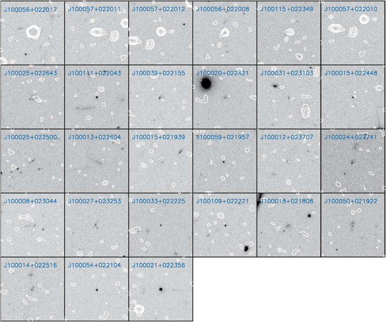
Figure 10. 10'' × 10'' postage stamps in the HST/ACS I-band for all the targets in the z = 2.47 protocluster observed with ALMA. All the cutouts are centered at the optical position of each galaxy. The white contours show the 2, 3, 4.5, 6, and 10σ of ALMA Band 6 (ν = 233 GHz, λ ≈ 1.3 mm) observations. The ID of each source is on the top of each panel.
Download figure:
Standard image High-resolution imageFootnotes
- 12
- 13
- 14
The average depth of σ ≈ 150 μJy at 870 μm of the observations used by Scoville et al. (2016) scales to ∼50 μJy at the wavelength used in this work, assuming the Rayleigh–Jeans relation and an emissivity index of β = 1.5. Similarly, the depth of the map presented in Dunlop et al. (2017) corresponds to ∼45 μJy These values are in good agreement with the depth of our observations (see Section 2.2). The work by Bouwens et al. (2016) is, however, based on observations a factor of ∼3× deeper.
- 15
Note that the mass-weighted age estimated by MAGPHYS depends not only on the time since the onset of star formation, but also on the shape of the star formation history. In the model, this quantity is typically ∼1.2× larger than the R-band light-weighted ages, the ages of the stars dominating the rest-frame R-band light (see details in da Cunha et al. 2015).
