Exploring the Galactic Warp through Asymmetries in the Kinematics of the Galactic Disk

Disk warps are common features of spiral galaxies (Bosma 1978; Binney 1992), and the presence of a warp in the outer Milky Way disk has long been established, as seen in its H i (e.g., Kerr 1957; Westerhout 1957; Weaver 1974; Levine et al. 2006; Voskes & Butler Burton 2006), dust (Freudenreich et al. 1994), star-forming regions (Wouterloot et al. 1990), and stellar disk components (e.g., Amôres et al. 2017 and references therein). The ubiquity of warps suggests that they are either repeatedly regenerated or long-lived phenomena in the lives of galaxy disks (Sellwood 2013).

While the origin of the Galactic warp still invites controversy, the fact that the stellar warp follows the same topology as the gaseous one is evidence that the warp is gravitationally induced (e.g., Miyamoto et al. 1988; Drimmel et al. 2000). Interactions with massive satellite galaxies can also affect the outskirts of galaxy disks, where the most likely candidates to create a warped outer disk in the Milky Way are the Sagittarius (Sgr) dwarf spheroidal (dSph) galaxy (Ibata & Razoumov 1998; Laporte et al. 2019) and the Magellanic Clouds (Weinberg & Blitz 2006; Garavito-Camargo et al. 2019). External torques on galaxy disks have also been identified with the accretion of intergalactic matter (Ostriker & Binney 1989; Wang et al. 2020), intergalactic magnetic fields (Battaner et al. 1990; Guijarro et al. 2010), and misaligned dark halos (Sparke & Casertano 1988; Widrow et al. 2014; Amôres et al. 2017). Moreover, disk instability has also been attributed to the cause of the warp. For instance, Chen et al. (2019) probed line-of-node twisting of the Galactic warp with classical Cepheids and suggested that the warp originated from the torques from the massive inner Galactic disk.

While the origin of the Galactic warp understandably remains a complex puzzle, simply defining the geometry of the warp is a problem that is also far from resolved, with a variety of potential models posited for its shape (Romero-Gómez et al. 2019). Even something as seemingly straightforward as the radius of the onset of the Galactic warp is still under debate. For example, Drimmel & Spergel (2001) found the onset of the warp to lie ∼1 kpc inside the solar circle using a three-dimensional model for the Milky Way fitted to the far-infrared (FIR) and near-infrared (NIR) data from the COBE/DIRBE instrument, a result supported by Huang et al. (2018) using stars from TGAS-LAMOST. Schönrich & Dehnen (2018), using the Tycho–Gaia Astrometric Solutions (TGAS) data set, also claimed that the warp begins inside the solar circle. On the other hand, population synthesis models from Derriere & Robin (2001) and Reylé et al. (2009) placed the onset of the Galactic warp at or outside the solar circle (see also Romero-Gómez et al. 2019, discussed further below).

In addition, the precession rate of Galactic warp is also unsettled. Drimmel et al. (2000) claimed that the warp is precessing rapidly (about 25 km s⁻¹ kpc⁻¹) in the direction of Galactic rotation, though the authors also acknowledge that the biased photometric distance caused the observed vertical motion to be smaller than their true values, mimicking the signal of precession. On the other hand, Bobylev (2010) analyzed the three-dimensional kinematics of about 82,000 Tycho-2 stars belonging to the red giant clump (RGC) and claimed that no significant precession of the warp is detected in the solar neighborhood. Most recently, Poggio et al. (2020) applied the precessing warp model from Drimmel et al. (2000) to Gaia DR2 data with the warp starting radius, height, and shape (R_w, h_w, and α) fixed to values in previous studies and reported that the warp is precessing at 10.46 km s⁻¹ kpc⁻¹, i.e., roughly half the rate found by Drimmel et al. Yet still more complicated are the definition of warp parameter dependencies as a function of stellar age, which may bear on the evolution of the warp or on the relative responses of different stellar populations to perturbations. For example, Amôres et al. (2017), using 2-Micron All Sky Survey (2MASS; Skrutskie et al. 2006) data and the Besançon Galaxy Model (Czekaj et al. 2014), identified a clear dependence of the thin-disk scale length as well as the warp and flare shapes with age. Meanwhile, the recent availability of enormous samples of Milky Way stars with precise 3D kinematics coming from the second data release of Gaia (Gaia DR2; Gaia Collaboration et al. 2018) has enabled much more comprehensive analyses of Galaxy dynamics over large ranges of Galactocentric radius, with the added means to estimate ages for field stars and with much greater statistical robustness for both. For instance, Poggio et al. (2018), using a combined sample of Gaia DR2 and 2MASS photometry, found the presence of a warp signal in two stellar samples having different typical ages and suggested that this means the warp is a gravitationally induced phenomenon. Shortly thereafter, Romero-Gómez et al. (2019) used two populations of different ages—young (OB-type) stars and intermediate-old age (red giant branch, RGB) stars—selected from Gaia DR2 and reported different onset radii for the Galactic warp for each, namely 12–13 kpc for the young sample versus 10–11 kpc for the older sample. These authors also report that the older sample reveals a slightly lopsided warp, i.e., the warp is not symmetric in shape about the plane, with a possibly twisted line of nodes.

One of the significant outcomes of this new capability in Galactic astronomy is the mapping of stellar motions—and asymmetries in those motions—across the Milky Way disk (e.g., Kawata et al. 2018; Poggio et al. 2018; López-Corredoira et al. 2020). Such kinematical asymmetries would be expected in the presence of a warp, but they can also explain smaller-scale features. For example, Bennett & Bovy (2019) and Carrillo et al. (2019) each reported a combination of bending and breathing modes using stellar kinematics derived from Gaia astrometry and confirmed that the Galactic disk is undergoing a wave-like oscillation with a dynamically perturbed local vertical structure within the solar neighborhood.

Such oscillatory motions may also explain various low-latitude substructures that reside in the outer Galactic disk, like the Monoceros ring (Newberg et al. 2002), Triangulum-Andromeda (TriAnd; Rocha-Pinto et al. 2004; Majewski et al. 2004), A13 (Sharma et al. 2010; Li et al. 2017), and other ring-like overdensities (Peñarrubia et al. 2005), whose origins have long been debated. For example, Monoceros and TriAnd were originally thought to be low-latitude tidal debris from dwarf galaxies (Chou et al. 2010; Sollima et al. 2011; Sheffield et al. 2014). However, there is now mounting chemical and kinematical evidence that some of these overdensities belong to the disk of the Milky Way (Bergemann et al. 2018; Hayes et al. 2018; Sales Silva et al. 2019; J. V. Sales Silva et al. 2020, in preparation) and represent concentrations of stars at the crests or troughs of ripple-like density waves in the Galactic disk or vertical oscillations of the Milky Way midplane at large Galactocentric radii that are excited by orbiting dwarf galaxies (e.g., Kazantzidis et al. 2008; Newberg & Xu 2017; Laporte et al. 2018; Bland-Hawthorne et al. 2019). If these overdensities are related to the local vertical structure of the Milky Way disk, they may therefore provide further constraining power on the source of these perturbations.

In this study, we use Gaia DR2 and APOGEE together with the StarHorse distance solutions (Anders et al. 2019) to explore vertical and radial velocity patterns and structures in the kinematics of the Galactic disk and to use these features to characterize the onset radius and precession rate of the warp. In Section 2, we describe the sources of our data, the distances adopted, and the conversion to the Galactocentric reference frame. In Section 3, we present several detected kinematical signatures in vertical and radial velocity, and in Section 4, we apply a simple model, based on the Jeans equation, to characterize these findings. In Section 5, we compare the responses to the galactic warp in four different age populations. In Section 6, we present the main conclusions from our analysis and outline prospects for building on the present work.

The data in this paper come primarily from Gaia DR2 (Gaia Collaboration et al. 2016, 2018) and the Apache Point Observatory Galactic Evolution Experiment (APOGEE & APOGEE-2; Majewski et al. 2017), part of SDSS-III (Eisenstein et al. 2011) and SDSS-IV (Blanton et al. 2017). We use these two primary sources to generate two different data sets for our analysis of the Galactic warp.

The first data set uses information for the 7,224,631 stars down to G ≃ 13 for which Gaia DR2 provides full six-dimensional phase-space coordinates: positions (α, δ), parallaxes (ϖ), proper motions (${\mu }_{\alpha }^{* }={\mu }_{\alpha }\cos \delta$, μ_δ), and radial line-of-sight velocities (v_los; Cropper et al. 2018). From that catalog, stars with suspect photometry and stars where the v_los measurement is based on fewer than four Gaia transits are removed. In addition, we decontaminate our sample of stars from the Large Magellanic Cloud (LMC) and Small Magellanic Cloud (SMC) by removing any sources within 5° of the center of these systems.

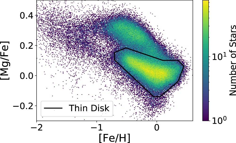
Our second data set is smaller, combining the proper motion, parallax and photometric information from Gaia DR2 with the chemical and radial velocity information from the latest public release of data from the APOGEE-2 survey, as contained in Sloan Digital Sky Survey (SDSS) Data Release 16 (DR16 Ahumada et al. 2020). DR16 contains high-resolution spectroscopic observations from both the Northern and Southern Hemispheres taken with the twin APOGEE instruments (Wilson et al. 2019) on the Sloan 2.5 m (Gunn et al. 2006) and the du Pont 2.5 m (Bowen & Vaughan 1973) telescopes, respectively. Individual stellar atmospheric parameters and chemical abundances are derived from the APOGEE Stellar Parameter and Chemical Abundance Pipeline (ASPCAP; García Pérez et al. 2016). For SDSS DR16, ASPCAP has been updated to use a grid of MARCS stellar atmospheres (Jönsson et al. 2020) and a new H-band line list from V. V. Smith et al. (2020, in preparation), all of which are used to generate a grid of synthetic spectra against which the target spectra are compared to find the best match (e.g., Zamora et al. 2015). From the full APOGEE sample, we require all sources to have the APOGEE STARFLAG and ASCAPFLAG set to "0" and to have an effective temperature between 3700 and 5500 K. A further restriction in [Fe/H] and [Mg/Fe] was made to only keep stars having chemistry characteristic of stars in the thin disk (see e.g., Bensby et al. 2014; Hayes et al. 2018), as illustrated and defined in Figure 1. The adopted thin-disk selection criterion is defined very conservatively, to limit contamination by non-thin-disk stars.

Zoom In Zoom Out Reset image size

In this study, we use distances derived through Bayesian inference using the StarHorse code (Queiroz et al. 2018). StarHorse combines precise parallaxes and optical photometry delivered by Gaia DR2 with the photometric catalogs of Pan-STARRS1 (Chambers et al. 2016), 2MASS (Skrutskie et al. 2006), and AllWISE (Wright et al. 2010), aided by the use of informative Galactic priors (Santiago et al. 2016; Queiroz et al. 2018). For the APOGEE data set, we use the StarHorse distances and extinctions from the APOGEE-2 DR16 StarHorse Value Added Catalog (Queiroz et al. 2020). The latter combines high-resolution spectroscopic data from APOGEE DR16 with the broad-band photometric data from the above sources and the Gaia DR2 parallaxes. Following the recommendation in Queiroz et al. (2020), we adopt the combination of SH_GAIAFLAG==''000'' and SH_OUTFLAG==''00000'' to filter out stars that have a problematic Gaia photometric or astrometric solution or a troublesome StarHorse data reduction.

The mean distance uncertainties for stars in our Gaia/Gaia–APOGEE samples are 0.24/0.42 kpc, and the mean relative uncertainties of distance are ∼8/10%. The mean uncertainty for the proper motions are 0.06/0.06 mas yr⁻¹ for the R.A. and decl. directions, respectively. Meanwhile, the mean uncertainties for the radial velocities are 1.69 km s⁻¹ for those coming from Gaia, and 0.21 km s⁻¹ for those from APOGEE. The total number of stars in the Gaia and Gaia–APOGEE data sets are 5,460,265 and 179,571, respectively.

The Galactocentric coordinate system adopted in this paper is right-handed, with the Sun at (X, Y, Z) = (−8.12, 0, 0.02) kpc (Gravity Collaboration et al. 2018; Bennett & Bovy 2019), a local standard of rest (LSR) velocity V_LSR = 233.4 km s⁻¹ (Reid & Brunthaler 2004; Gravity Collaboration et al. 2018), and a solar velocity relative to the LSR of V_⊙ = (12.9, 12.24, 7.78) km s⁻¹ (Drimmel & Poggio 2018). Note that in this adopted Galactocentric Cartesian coordinate system, Galactic rotation converts to a negative azimuthal velocity (v_ϕ) when expressed in cylindrical coordinates. For this reason, in many of the figures presented below, we adopt  − L_z for the abscissa.

Under this coordinate system, the spatial distribution of stars in our samples is shown in Figure 2. As may be seen, both of our samples have kinematical information extending to ∼10 kpc from the Sun, although most of the stars are concentrated in the disk, within Z = ±3 kpc of the Galactic plane. The presence of the Galactic bar and bulge starts becoming evident at X ≲ −4 kpc. The presence of the Galactic bar and bulge starts becoming evident at X < −4 kpc in our data, as already reported by Anders et al. (2019), Queiroz et al. (2020), and A. B. A. Queiroz et al. (2020, in preparation) using the StarHorse distance solution. As expected, the all-sky Gaia sample is more smoothly and completely distributed, while the Gaia–APOGEE sample shows the pencil-beam spikes corresponding to the field-by-field coverage of the APOGEE and APOGEE-2 surveys, as well as the more limited coverage in the Southern Hemisphere, where APOGEE only began observing more recently in APOGEE-2.

Zoom In Zoom Out Reset image size

3.1. The General Trend and Ripples in Vertical Velocity

The warp and its kinematical signature are expected to be more prominent toward the Galactic anticenter and evident by large-scale systemic stellar motions perpendicular to the plane (e.g., Binney 1992; Drimmel et al. 2000). Our Gaia and Gaia–APOGEE samples, in combination with the StarHorse distances, allow us to characterize the stellar vertical motion over a large range of Galactocentric radius, where we are able to explore to R_GC ∼ 18 kpc. Here we study the kinematical signature of the Galactic warp in our two stellar samples, specifically by exploring the vertical velocity v_z in the disk as a function of angular momentum (L_z) and Galactocentric radius (R), as was done previously by Schönrich & Dehnen (2018) and Huang et al. (2018). In addition, we look for any azimuthal asymmetries in these trends.

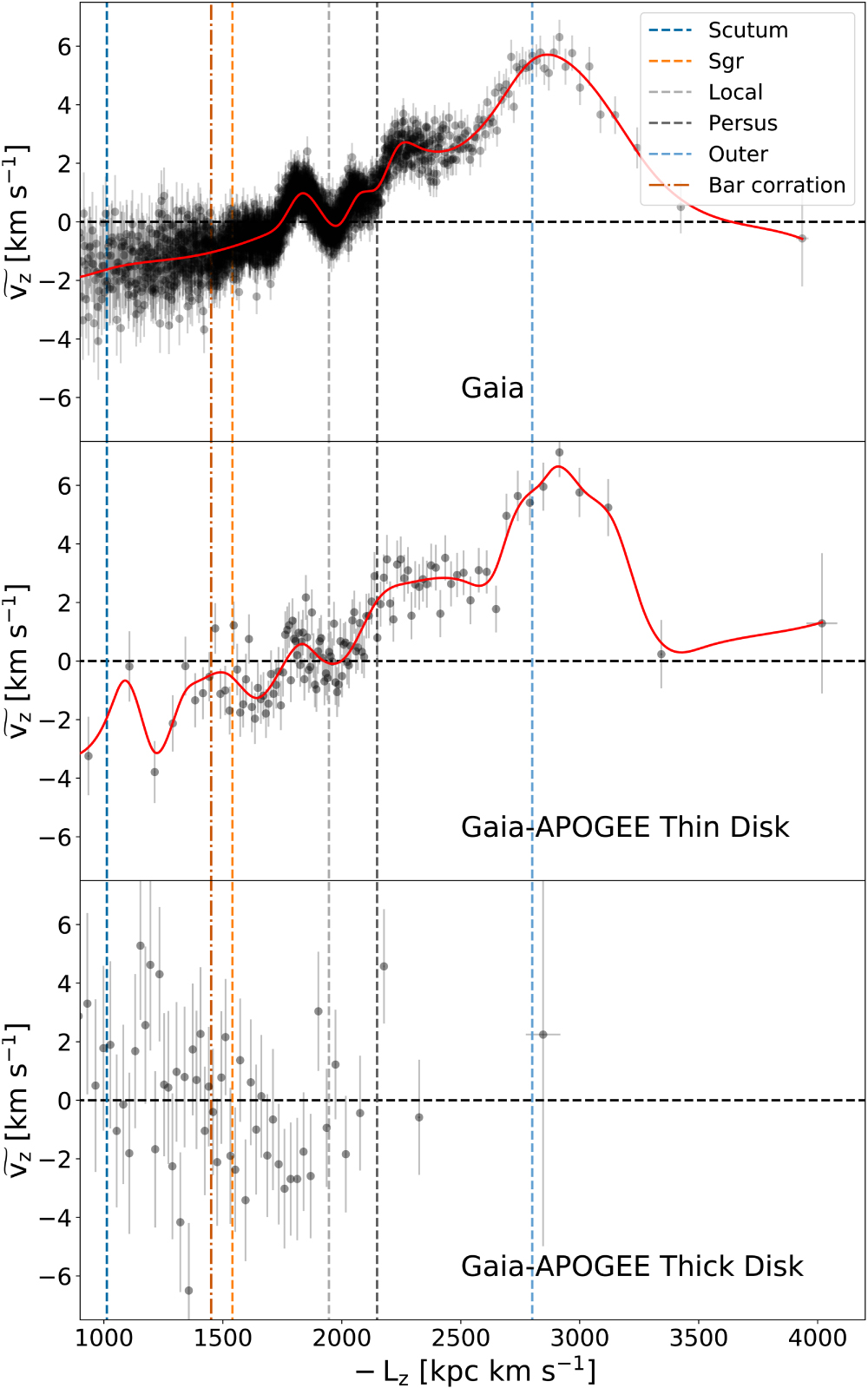
Figure 3 shows the run of $\widetilde{{v}_{z}}$ with L_z for the Gaia data set (in the left panel) and the chemically selected thin-disk stars from the Gaia–APOGEE sample (in the right panel). Stars in Figure 3 are sorted and binned by angular momentum, with each point representing 2000 stars for the former data set, and, because the parent sample is smaller, each point represents 1000 stars for the Gaia–APOGEE sample. The error bars represent the uncertainty of the median value, which have been estimated through bootstrapping: 1000 subsamples containing 80% of the stars in each bin were randomly drawn and the standard deviation of the median of these subsamples were taken as the error of the median.

Zoom In Zoom Out Reset image size

The trend of the Gaia sample (top panel of Figure 3) strongly resembles that of the Gaia–APOGEE sample (middle panel). Because the latter was deliberately chosen via chemistry (Figure 1) to select thin-disk stars, we can conclude that the features shown in the larger Gaia sample are driven by thin-disk stars. This conclusion is reinforced by the trend of the thick-disk stars (bottom panel), which does not at all resemble the trend of the Gaia stars.

Figure 3 shows that over a large range of L_z, the overall mean vertical velocity increases with L_z, starting at −2 km s⁻¹ and peaking at around +6 km s⁻¹. This velocity increase is more pronounced for values larger than L_z > 1800 kpc km s⁻¹ and continues until L_z ∼ 2800 kpc km s⁻¹, after which $\widetilde{{v}_{z}}$ sharply declines. A general increasing trend of $\widetilde{{v}_{z}}$ with L_z was also noted by Schönrich & Dehnen (2018) and Huang et al. (2018). However, while these previous studies reported that the correlation between $\widetilde{{v}_{z}}$ and L_z can be approximated by a rising linear fit over their entire sample, our more extensive radial coverage of disk kinematics reveals that the increasing trend is limited to L_z ≲ 1800 kpc km s⁻¹, beyond which $\widetilde{{v}_{z}}$ actually declines. We believe that this entire global trend in $\widetilde{{v}_{z}}$ is the signature of the Galactic warp, and we further characterize it and model it as such in Section 4.

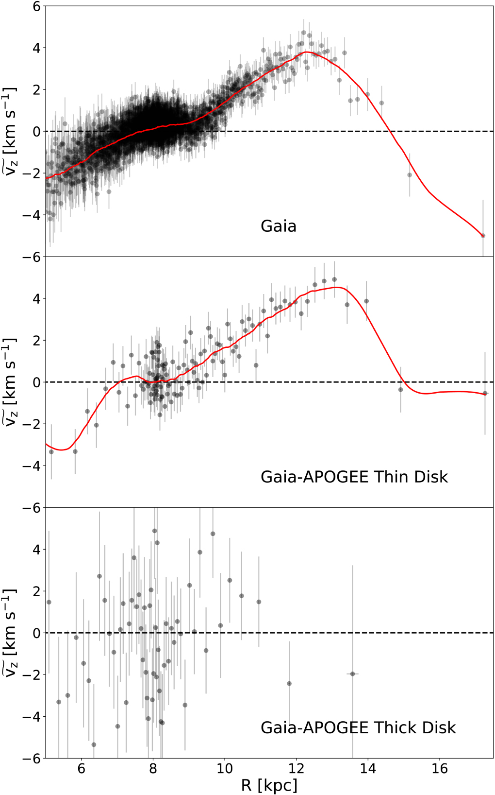
Figure 3 also reveals, superposed on top of this general trend, higher frequency, wave-like ripples in $\widetilde{{v}_{z}}$ as a function of L_z. The source of these $\widetilde{{v}_{z}}$ ripples is more elusive (and will be explored after examination of similar trends in radial velocity, discussed in Section 3.2). However, these ripples are less prominent in the vertical velocity versus Galactocentric radius plot (Figure 4): although the general trend of vertical velocity first increasing and then decreasing as Galactocentric radius increases is still evident, the ripples, especially those at solar radius, are smeared out in this representation. We argue that the reason the ripples are present in Figure 3 but not in Figure 4 is because angular momentum is conserved for stars but for a given present-day radius, you have a mix of stars at different phases in their orbits. Therefore, after stars have made a few revolutions around the Galactic center, any initial spatial patterns would smear out when binned in Galactocentric radius, even while L_z is preserved.

Zoom In Zoom Out Reset image size

An asymmetry in the Galactic H I warp has been extensively studied (Burke 1957; Baldwin et al. 1980; Henderson et al. 1982; Richter & Sancisi 1994), but whether there is a similar effect on the stellar disk is less understood. Recently, Romero-Gómez et al. (2019) reported asymmetry in the mean vertical distance of the stars from the Galactic plane about the warp line of nodes at ϕ ≈ 180°, with the warp-down amplitude (at ϕ ≳ 180°) being larger than the warp-up amplitude (at ϕ ≲ 180°), i.e., that the warp is lopsided. Such differences in the amplitude of the spatial distribution may correlate to an asymmetry in the azimuthal variation of the vertical velocity between the up and down sides of the warp. Furthermore, previous research also probed the possibility that the peak maximum vertical velocity is not in the anticenter direction (Yusifov et al. 2004; Skowron et al. 2019; Li et al. 2020). To verify these presumptions, we plot the median vertical velocity as a function of Galactocentric azimuth angle, ϕ, for different radial annuli in Figure 5. At Galactocentric radii around the solar neighborhood, we see that the vertical velocity is relatively constant as a function of azimuthal angle, but at larger radii, we begin to see substantial differences in the vertical velocities at different azimuths. In particular, the vertical velocity first increases as ϕ increases, reaches a maximum vertical velocity peak or plateau around ϕ ≈ 170°, and then decreases with increasing ϕ. Furthermore, the increasing and decreasing slopes of the vertical velocity with ϕ appear to be asymmetric about this peak or plateau, with a steeper decline in vertical velocity at ϕ > 170° than the increase at ϕ < 170°. For a warp with an equal warp-up and warp-down amplitude, the vertical velocity should be symmetric about the longitude of peak vertical velocity; that this is not seen further indicates that the warp is lopsided, as previous studies have identified using the altitude with respect to the Galactic plane at a given Galactocentric radius (e.g., Marshall et al. 2006; Romero-Gómez et al. 2019).

Zoom In Zoom Out Reset image size

To illustrate further the kinematical lopsidedness of the Galactic warp, we directly measure the velocity asymmetry by subtracting the median vertical velocity of stars on one side of ϕ_peak from its complement on the other side at the same azimuthal separation for each radial annulus (Figure 6), and ϕ_peak is estimated within each radial annulus by using a wider bin (10°) between 160° < ϕ < 200°. For every radial annulus, except the one with R > 13.5 kpc, we find a steadily increasing difference in vertical velocity when moving away from the peak, which is expected from a lopsided warp.

Zoom In Zoom Out Reset image size

3.2. Ripples in Radial Velocity and Their Potential Origin

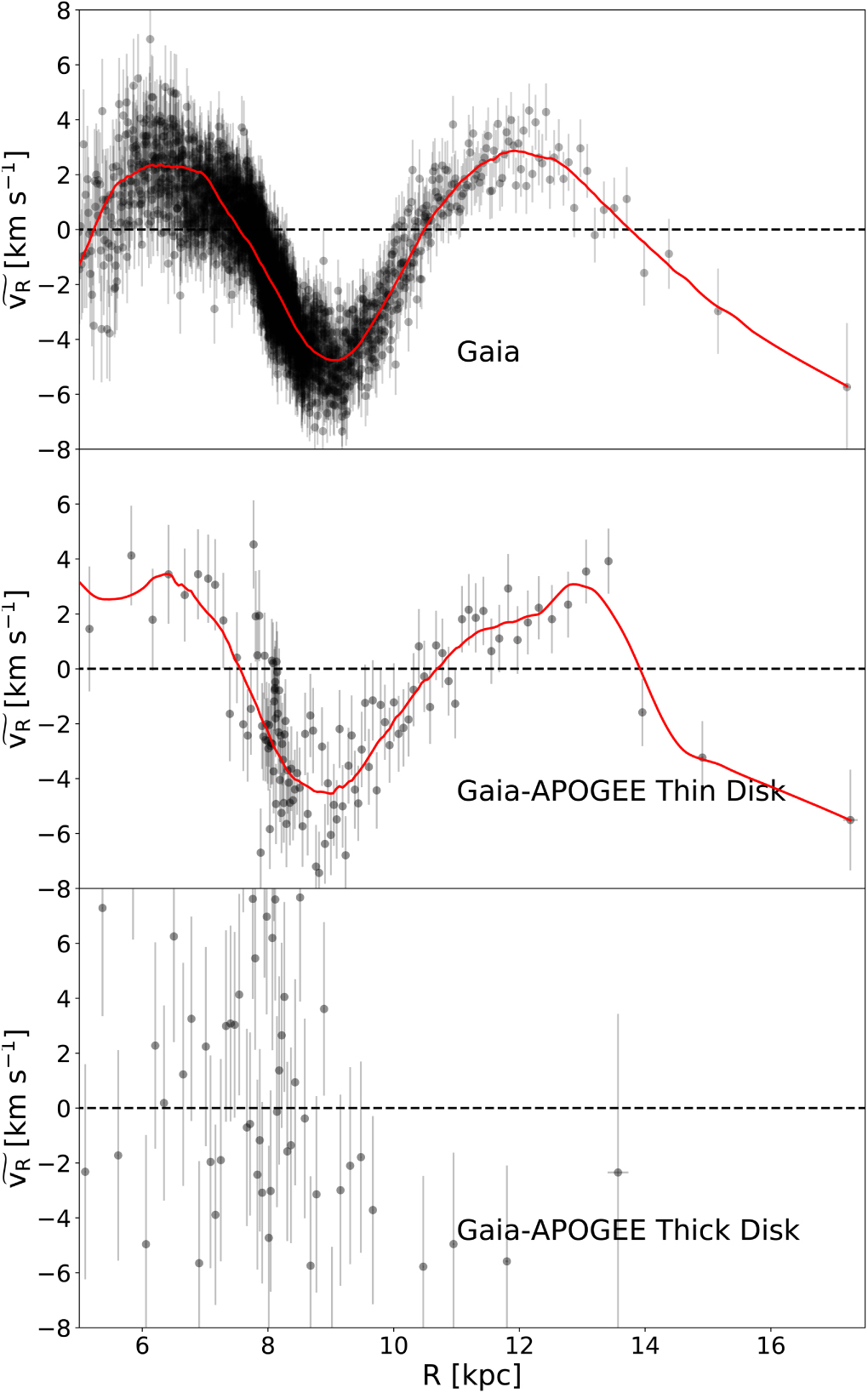
Figures 7 and 8 show the complementary stellar radial motions with respect to L_z and R, respectively. Here, again, a pattern of ripples is seen, and they are even more dramatic, reaching more extreme velocity amplitudes. As was observed with the v_z trends (i.e., Figures 3 and 4), (a) the trends of the Gaia sample are best matched by the Gaia–APOGEE thin-disk sample rather than the thick-disk sample, and (b) the v_R ripples seen when plotted as a function of L_z are smeared out when plotted as a function of Galactocentric radius. Such a kinematical pattern for v_R was also reported for very young OB stars alone when viewed with respect to Galactocentric radius (Cheng et al. 2019).

Zoom In Zoom Out Reset image size

Zoom In Zoom Out Reset image size

Two possible mechanisms have previously been proposed to lead to such observed ripples. One explanation for these localized features is that they may be related to spiral arm perturbations, where the mass enhancements associated with spiral density waves can gravitationally scatter stars (e.g., Jenkins & Binney 1990). To illustrate the potential connection of these oscillations to spiral arms, in Figure 3 we indicate the angular momentum values of the known Milky Way spiral arms, calculated as follows: first, we take the parameters that characterize these spiral arms from Reid et al. (2014). Then, a number of equally spaced points were generated within the Galactocentric radius and azimuthal angle range of each spiral arm. The standard rotation curve from Bovy (2015) is assumed and used to calculate the azimuthal velocity. The angular momentum for each point is then computed and a variety of statistics (median, standard deviation, min/max values) generated to describe each spiral arm (see Table 1). We also show the L_z position corresponding to the Galactic bar, where we assume a pattern speed of Ω = 39.0 km s⁻¹ kpc⁻¹ (Portail et al. 2017).

Table 1.  Summary of the Vertical Angular Momentum Properties for Different known Milky Way Spiral Arms, Calculated as Described in Section 3.1

Spiral arm	$\widetilde{{L}_{z}}$ (kpc km s−1)	${\sigma }_{{L}_{z}}$ (kpc km s−1)	Minimum Lz (kpc km s−1)	Maximum Lz (kpc km s−1)
Scutum	1012	202	661	1427
Sagittarius	1540	85	1374	1705
Local	1945	98	1755	2136
Perseus	2148	191	1783	2541
Outer	2800	225	2364	3264

Note. The second and third columns are the median angular momentum and corresponding standard deviation for each spiral arm. The fourth and fifth columns are the minimum and maximum angular momenta of the points associated with each spiral arm.

Download table as:  ASCIITypeset image

After performing this simple exercise, we find (Figure 3) that even though the nominal Perseus and Outer Arms correspond to the local maximum of the vertical ripples, the Scutum, Sgr, and Local Arms do not. In terms of radial motion (Figure 7), there are many v_R features that appear to be matched to corresponding v_z features at the same L_z, and some correlations between the L_z positions of some ripples and those characteristic of spiral arms can be seen—in particular, once again, between the L_z ∼ 1950 kpc km s⁻¹ valley and the Local Spiral Arm and the peak at L_z ∼ 2150 kpc km s⁻¹ with the Perseus Spiral Arm, but in this case no correlation between the Outer Spiral Arm and a v_R feature is seen. We expect spiral arms to couple more tightly with the radial motions of stars, making the radial velocity dispersion significantly greater than the velocity dispersion perpendicular to the plane (e.g., Jenkins & Binney 1990; Aumer et al. 2016). However, while most spiral arms correspond to maximum positive velocity, the Local Arm is at the point of maximum negative velocity. It is also apparent that some ripples visible in these figures do not correlate with known spiral arm patterns, while some spiral arms (in particular, those at smaller L_z) do not match observed ripples. While these discrepancies might suggest that the ripples are not (or not entirely) generated by spiral arms, such lack of one-to-one correlation may also reflect shortcomings of the above illustrative exercise and the many uncertainties and simple assumptions used to generate it.

Another mechanism to produce the ripples that has been proposed is perturbations of the disk caused by satellite galaxies. It has been suggested that the Galactic disk oscillates vertically due to radially propagating waves—i.e., bending waves caused by the passing of orbiting Milky Way satellites (Hunter & Toomre 1969), such as the Sgr dSph (Ibata & Razoumov 1998; Laporte et al. 2018; Darling & Widrow 2019). Some success in modeling these features in the stellar disk (but for more limited empirical mappings of Milky Way features than presented here) has been shown by Widrow et al. (2014) and Laporte et al. (2019), who invoke a semianalytical prescription and N-body simulation of the Sgr dwarf galaxy interacting with the Galactic disk to explain the oscillatory disk star patterns. In both cases, regardless of the mass of the impactor, changes in vertical velocity on the scale of 5 km s⁻¹ within R < 20 kpc in the anticenter direction are observed, especially in Laporte et al. (2019), where their model L2 exhibits a strikingly similar overall trend to that of the observations, with vertical velocity increasing with Galactocentric radius over 5 < R < 10 kpc to a maximum value of ∼5 km s⁻¹, and then decreasing with Galacocentric radius over radii 13 < R < 20 kpc.

Meanwhile, in N-body simulations of passages of massive satellite galaxies around a Milky Way–like disk galaxy, D'Onghia et al. (2016) find an increasing vertical velocity over 5 < R < 10 kpc and decreasing vertical velocity for 13 < R < 20 kpc, as well as some smaller ripples within 7 < R < 10 kpc. Ripples in the radial dimension as large as 20 km s⁻¹ have been detected in the D'Onghia et al. (2016) simulations that are attributable to the Galactic warp itself.

At present, we offer no definitive explanation for the fine structure seen in the kinematical trends in Figures 3 and 7. Like Schönrich & Dehnen (2018), Huang et al. (2018), and Friske & Schönrich (2019), we point out these high-frequency kinematical features but do not offer a physical model to explain them. On the other hand, we find that either (or both) the spiral arm and/or satellite perturbation scenario seems viable. For the remainder of the analysis here, we focus on attempting to describe the more global trends visible in Figures 3–8)—in particular, the large-scale trends one might expect to be produced by a large disk warp.

We can treat stars as a collisionless fluid and apply the first Jeans equation to link the kinematics of Galactic stars to their number density through the collisionless Boltzmann equation (CBE hereafter; Jeans 1915; Henon 1982). A simple analytical model for the Galactic warp can be derived using the CBE (e.g., Equation (11) in Drimmel et al. 2000), after adopting several simplifying assumptions. Here we follow the Drimmel et al. (2000) approach, but without making as many simplifications. For example, Drimmel et al. assume there are no net radial motions, i.e., v_R = 0. However, our data sets binned in vertical angular momentum, L_z, and Galactocentric radius, R (see Figures 7 and 8, respectively), show an even larger velocity range in the radial direction (from −5 to 7 km s⁻¹) than in the vertical direction (from −4 to 4 km s⁻¹) at R > 6 kpc. Therefore, we build a similar model to that of Drimmel et al. (2000), but one that accounts for a nonzero radial motion, v_R. While our model attempts to take another step in the degree of sophistication, it is still very simple and does not capture all of the possible physics. In particular, it does not include warp lopsidedness.

The essence of the model is to treat the Galactic warp as a perturbation in the Milky Way disk. For an unperturbed (nonwarped) disk, one can assume perfect axisymmetry for simplicity, eliminating the dependence of the unperturbed parameters on the Galactocentric azimuthal angle, ϕ. Moreover, one can assume that the unperturbed number density is a separable function with respect to Galactocentric radius R and distance from the Galactic plane z:

$$\begin{eqnarray}&&n(R,z)=f(R)g(z).\end{eqnarray} \tag{ 1 }$$

In this circumstance, the addition of a Galactic warp perturbation would only have an effect on the vertical direction. Namely, stars that reside at a given position (R, ϕ, z) are deviated by z₀(R, ϕ, t). Therefore, the perturbed number density of stars can be written as

$$\begin{eqnarray}&&n^{\prime} (R,\phi ,z)=n(R,z-{z}_{0})=f(R)g(z-{z}_{0}).\end{eqnarray} \tag{ 2 }$$

Accounting for the warp, according to Drimmel et al. (2000), one could write z₀ as

$$\begin{eqnarray}&&{z}_{0}=h(R)\sin (\phi -{\phi }_{w}+{\omega }_{p}t),\end{eqnarray} \tag{ 3 }$$

where h(R) is the deviation from the Galactic midplane at a given Galactocentric radius R, ϕ is the Galactocentric azimuthal angle, ϕ_w is the line of nodes at present day (t = 0)—i.e., where there is no vertical displacement (z₀ = 0)—and ω_p is the precession rate of the warp.

An analytical form of h(R) is given in Drimmel et al. (2000), but Romero-Gómez et al. (2019) pointed out that a model with an ending radius of the Galactic warp and flexible exponents in h(R) would reproduce observed kinematical patterns better. Thus, we adopt a new analytical form of h(R) by merging the models from these two above-mentioned sources:

$$\begin{eqnarray}h(R)=\left\{\begin{array}{ll}0 & R\leqslant {R}_{1}\\ \tfrac{{R}_{w}}{{R}_{2}-{R}_{1}}{\left(R-{R}_{1}\right)}^{\alpha } & {R}_{1}\lt R\leqslant {R}_{2}\\ h({R}_{2})+\tfrac{{dh}}{{dR}}{| }_{R={R}_{2}}(R-{R}_{2}) & R\gt {R}_{2}\end{array}\right.,\end{eqnarray} \tag{ 4 }$$

where R₁ is the starting radius of the warp, R₂ is the ending radius of the warp, R_w is a scale factor for the warp height, and the exponent α characterizes the shape of the warp. We can write the first Jeans equation in cylindrical coordinates as

$$\begin{eqnarray}&&\displaystyle \frac{\partial n^{\prime} }{\partial t}+\displaystyle \frac{\partial (n^{\prime} \overline{{v}_{R}})}{\partial R}+\displaystyle \frac{1}{R}\displaystyle \frac{\partial (n^{\prime} \overline{{v}_{\phi }})}{\partial \phi }+\displaystyle \frac{\partial (n^{\prime} \overline{{v}_{z}})}{\partial z}=0.\end{eqnarray} \tag{ 5 }$$

However, because v_ϕ is not perturbed by the warp, one can still apply the axisymmetric condition, so that ${\rm{\partial }}\bar{{v}_{\phi }}/{\rm{\partial }}\phi =0$. We also adopted the assumption ${\rm{\partial }}\bar{{v}_{z}}/{\rm{\partial }}z=0$ made by Drimmel et al. (2000) for simplicity. After using the product rule of derivatives and applying the above assumptions, one finds

$$\begin{eqnarray}&&\begin{array}{l}[\overline{{v}_{z}}-\left(\displaystyle \frac{\overline{{v}_{\phi }}}{R}+{\omega }_{p}\right)h(R)\cos (\phi -{\phi }_{w}+{\omega }_{p}t)\\ \quad -\,\overline{{v}_{R}}\displaystyle \frac{{dh}}{{dR}}\sin (\phi -{\phi }_{w}+{\omega }_{p}t)]f(R)\displaystyle \frac{{dg}}{{dz}}\\ \quad +\,\overline{{v}_{R}}\displaystyle \frac{{df}}{{dR}}g(z-h(R)\sin (\phi -{\phi }_{w}+{\omega }_{p}t))\\ \quad +\,\displaystyle \frac{\partial \overline{{v}_{R}}}{\partial R}n^{\prime} =0.\end{array}\end{eqnarray} \tag{ 6 }$$

Unlike the more simplified treatment in Drimmel et al. (2000), here the factors $n^{\prime}$, f(R), and g(z) do not cancel out. We assume the initial mass function is a constant across the entire galaxy, so that the number density of stars is directly proportional to the mass density of the stellar disk. From the similarity in behavior displayed between the Gaia versus Gaia–APOGEE samples in Figure 3, we conclude that the outer disk, where the warp happens and which is the focus of our interest, is dominated by thin-disk stars; thus, we can safely assume the mass density follows a double-exponential potential like that followed by thin-disk stars. Thus, we assume

$$\begin{eqnarray}&&n(R,z)={n}_{0}\exp \left(-\displaystyle \frac{| z| }{{z}_{h}}-\displaystyle \frac{R}{{R}_{h}}\right),\end{eqnarray} \tag{ 7 }$$

where R_h is the scale length and z_h is the scale height of the thin disk.

Adopting this as the density and the assumption that ϕ_w = 180°, one then obtains a final equation that links together the different components of velocity:

$$\begin{eqnarray}\begin{array}{rcl}\displaystyle \frac{\partial \overline{{v}_{R}}}{\partial R} & = & \displaystyle \frac{\overline{{v}_{R}}}{{R}_{h}}+\displaystyle \frac{{sign}[z-{z}_{0}]}{{z}_{h}}\left[\overline{{v}_{z}}-\left(\displaystyle \frac{\overline{{v}_{\phi }}}{R}+{\omega }_{p}\right)h(R)\cos \theta \right.\\ & & \left.-\,\overline{{v}_{R}}\displaystyle \frac{{dh}}{{dR}}\sin \theta \right],\end{array}\end{eqnarray} \tag{ 8 }$$

where θ = ϕ − ϕ_w + ω_p t. Because we assume the distribution of the stellar population is symmetric about z₀, the final observed vertical velocity is the average of those with z > z₀ (where sign[z − z₀] = 1) and z < z₀ (where sign[z − z₀] = − 1), yielding

$$\begin{eqnarray}&&\overline{{v}_{z}}=\left(\displaystyle \frac{\overline{{v}_{\phi }}}{R}+{\omega }_{p}\right)h(R)\cos \theta +\overline{{v}_{R}}\displaystyle \frac{{dh}}{{dR}}\sin \theta .\end{eqnarray} \tag{ 9 }$$

The free parameters in our model are the Galactocentric radius where the warp starts and ends (R₁ and R₂, respectively), the scale height of the warp (R_h), and the precession speed of the warp (ω_p). This is in contrast to those of Poggio et al. (2020), where the only allowed free parameter is the precession rate of the warp. One finds that the best fit to the trend of vertical velocity with Galactocentric radius, as derived via a Markov Chain Monte Carlo method (MCMC), is described by

$$\begin{eqnarray*}&&\left\{\begin{array}{l}{\omega }_{p}=-{13.57}_{-0.18}^{+0.20}\ \mathrm{km}\ {{\rm{s}}}^{-1}\ {\mathrm{kpc}}^{-1}\\ {R}_{1}={8.87}_{-0.09}^{+0.08}\ \mathrm{kpc}\\ {R}_{2}={17.78}_{-1.86}^{+1.56}\ \mathrm{kpc}\\ {R}_{w}={1.20}_{-0.26}^{+0.28}\ {\mathrm{kpc}}^{2-\alpha }\\ \alpha ={1.53}_{-0.09}^{+0.10}.\end{array}\right.\end{eqnarray*}$$

The best fit is shown in Figure 9 in red, and the corner plot for MCMC fitting is shown in Figure 10. Notice that the model does not match well in the inner part of the Galaxy. This is expected for several reasons: first, we are only fitting our model for R > 8 kpc. Moreover, the Galactic warp would have a very limited effect in the inner (more massive) part of the Galaxy, rendering our model inappropriate there. Figure 10 also shows that the model is not sensitive to the ending radius of the warp R₂. We attribute that insensitivity to the low number of stars beyond R > 16 kpc.

Zoom In Zoom Out Reset image size

Zoom In Zoom Out Reset image size

Our result for ω_p is consistent with that of Poggio et al. (2020; again, for them, ω_p is the only free parameter, and we adopt an opposite sign convention for the direction of the precession term). While our model is very crude in construction, it illustrates the possibility of explaining the decline in vertical velocity as due to a warp precessing in the direction of Galactic rotation.

Even though such a decline was also observed by Drimmel et al. (2000), they attributed it to the extremely large uncertainty in distance for stars beyond the solar neighborhood. However, that does not appear to be the case here as the number of stars within each of our binned data points is significantly higher, which greatly reduces the uncertainty of the mean value.

Our result for the Galactocentric radius where the warp begins agrees well with previously reported values. A comparison of existing models, with trends in z with R shown at the maximum vertical distance from the Galactic midplane for each, is provided in Figure 11. However, while the latter figure shows that there is good agreement on R₁, there is also a large spread in the amplitude of the warp among the various models. Moreover, our model agrees better with those exhibiting a stronger warp. It is worth noting that the set of models by Amôres et al. (2017), to which we show the most agreement, has included more physics (e.g., flaring, disk truncation, star formation history, etc.) than the other models, including ours, which is a reassuring check on our model.

Zoom In Zoom Out Reset image size

In the past few years, there have been several lines of evidence suggesting that the parameters of the warp in the Milky Way disk change with the average age of the tracing stellar population (e.g., Drimmel et al. 2000; Amôres et al. 2017; Romero-Gómez et al. 2019; Poggio et al. 2020). In this section, we use the stellar age catalog provided by Sanders & Das (2018) to explore how different aged populations are warped differently. This catalog contains the ages of ∼3 million Gaia stars, derived using a Bayesian framework to characterize the probability density functions of age for giant stars with combined photometric, spectroscopic, and astrometric information, supplemented with spectroscopic masses, where available. We only include stars for which Sanders & Das set "flag = 0"; according to these authors, stars were assigned nonzero flags when (a) the isochrone fitting failed completely, (b) the isochrone overlapped with the data at only one point, (c) the spectroscopic or photometric input data are problematic, or (d) the derived ages are unreasonably small (<100 Myr).

We acknowledge one caveat is that these ages were derived from extrapolating the relation C/N with age at the solar vicinity. Although individual stars in the Sanders & Das (2018) catalog may have a large uncertainty in their estimated age (see Figure 12), these estimates are of sufficient quality to sort stars broadly by age and serve as a general indicator of the average age of a population when averaging over a significant number of stars. We selected stars in four age bins: those stars with ages 0–3 Gyr as a "young population," those with ages 3–6 Gyr as an "intermediate age population," those 6–9 Gyr in age as an "old population," and finally, those dated at >9 Gyr as an "ancient population."

Zoom In Zoom Out Reset image size

The mean vertical velocity versus angular momentum for each of these age groups is shown in Figure 13. It is clear that there are major differences in this particular kinematical trend between different aged populations. The young population (orange points in Figure 13) shows the largest increase in vertical velocity, and the maximum median v_z declines with increasing population age through the intermediate- and old-aged populations. The abrupt decline in median v_z is evident in all three populations with age <9 Gyr, albeit with slightly differing starting L_z for the beginning of the drop-off. For the ancient stars (brown points in Figure 13) the effect of the warp is less evident; this is likely due to the large number of halo stars within the ancient population. This conclusion is based on the character of the rotation curve exhibited by this population, which, unlike the younger star groups, shows a rapid decline beyond the solar circle Figure 15.

Zoom In Zoom Out Reset image size

We applied our simple analytical model to fit and track the changes of parameters of the warp with stellar age in Figure 14. However, because our model is limited in its complexity, it cannot account for ripples not associated with the Galactic warp or non-thin-disk stellar kinematics. As a result, fitting results are not reported for the youngest population, for which prominent substructures not related to the Galactic warp are attributable to the higher frequency ripples. Nor do we report a fit for the ancient population, where, as we have shown Figure 15, a substantial fraction of the sample is contaminated by halo stars.

Zoom In Zoom Out Reset image size

Zoom In Zoom Out Reset image size

On the other hand, for the 3–6 Gyr population, our fit yields a precession rate of $-{11.59}_{-0.25}^{+0.30}\ \mathrm{km}\ {{\rm{s}}}^{-1}\ {\mathrm{kpc}}^{-1}$, while for the 6–9 Gyr population, we obtain $-{12.19}_{-0.39}^{+0.49}\ \mathrm{km}\ {{\rm{s}}}^{-1}\ {\mathrm{kpc}}^{-1}$. The lack of any significant difference between these two populations suggests that the response to the warp in at least these two populations is similar. However, from Figure 13, a clear difference in the size of the vertical velocity is present between different age populations, with the older population being slower. This difference in amplitude could be consistent with the warp being a recent event (that is, within the past 3 Gyr), but where different aged populations respond differently in bulk: presumably, the older population, which is also the kinematically hotter population, would have a weaker response to dynamical perturbations.

Apart from differences in the amplitude of the warp in different populations, we also find that the peaks of vertical velocity are at different Galactocentric radius for different age populations (Figure 14). The peak vertical velocity is moving closer to the Galactic Center as the population grows older. One explanation for this is suggested by Figure 15, where a decrease in azimuthal velocity correlates to older populations; according to the factor (${v}_{\phi }/R+{\omega }_{p}$) in Equation (9), when the precession rate is similar between two populations, the population with smaller azimuthal velocity will have a peak closer to the Galactic Center. However, we also notice, curiously, that the fractional decrease in azimuthal velocity (that is, from ∼220 km s⁻¹ for the 3–6 Gyr population to ∼210 km s⁻¹ for the 6–9 Gyr population) is about a factor of 2 smaller than the fractional decrease in where the peak vertical velocity is located (∼13 kpc for the 3–6 Gyr population, ∼12 kpc for the 6–9 Gyr population), when these decreases should be proportional.

With no age-variable signatures in the precession of the warp but some differences in the velocity amplitude, it is worth testing whether there may be age-variable signatures in the lopsidedness of the warp that we previously found across the entire sample (Section 3.1). Figure 16 shows the azimuthal distribution of median vertical velocity in different age populations for different radial annuli. The lopsidedness is prominent in all age groups for radii beyond R > 7.5 kpc. Moreover, the lopsidedness remains similar, with the vertical velocity increasing when ϕ < 180° and decreasing when ϕ > 180°. The slope of the increase and decrease is also similar across the different age populations. This further supports that the different age population has a similar response to the Galactic warp, thus suggesting a possible gravitational origin.

Zoom In Zoom Out Reset image size

In the end, our consideration of potential age differences in the characteristics of the warp reveals them to be consistent with a model whereby the intermediate and older populations are both responding to a single gravitational perturbation happening less than 3 Gyr ago.

In this study, we combine the precise stellar abundances from the APOGEE survey with the astrometry from Gaia DR2 and the StarHorse distance computed by Queiroz et al. (2020) to study the vertical and radial velocity components of stars with respect to the Galactocentric radius and angular momentum. We take advantage of the detailed and accurate chemical abundances available in the smaller APOGEE–Gaia sample (Figure 1) as a guide to the interpretation of the much larger Gaia-only sample. Our analysis probes disk kinematics to a greater Galactocentric radius (R ∼ 18 kpc) than has been explored previously (Figure 2). From these combined data, we find evidence for the Galactic warp and characterize its onset radius and precession rate. Interestingly, a number of high spatial frequency kinematical features are also found, as has been reported by previous authors at smaller Galactocentric radii (Figures 3 and 7).

We find that over a large range of L_z, the overall median stellar vertical velocity ${\widetilde{v}}_{z}$ increases with L_z. Moreover, the increase of the mean vertical velocity is more pronounced for L_z > 1800 kpc km s⁻¹ and continues until L_z ∼ 2800 kpc km s⁻¹ or R = 13 kpc, after which the vertical velocity sharply declines (Figures 3 and 4). This abrupt decrease in $\widetilde{{v}_{z}}$ is reported for the first time. We associate this entire global trend in $\widetilde{{v}_{z}}$ as a signature of the Galactic warp. We also study the vertical velocity as a function of the Galactocentric azimuthal angle for the Gaia sample and found differences in this parameter with respect to the Galactocentric azimuthal angle for ϕ < 180◦ and ϕ > 180◦, evidence consistent with a warp line of nodes toward this anticenter direction (Figure 5). However, the velocity trends with ϕ in our data appear to be asymmetric about ϕ ∼ 180° (Figure 6), which is evidence suggesting that the Galactic warp may be lopsided.

An analytical model using the Jeans equation with consideration of a nonzero radial motion is constructed to explain the observed phenomena, and shows that the declining trend in vertical velocity can be explained as a manifestation of the Galactic warp. We find that the warp has a starting radius of ${8.87}_{-0.09}^{+0.08}\,\mathrm{kpc}$ and a precession rate of $-{13.57}_{-0.18}^{+0.20}\ \mathrm{km}\ {{\rm{s}}}^{-1}\ {\mathrm{kpc}}^{-1}$ (Figures 9 and 10), a value slightly higher than the 10.86 km s⁻¹ kpc⁻¹ reported recently in Poggio et al. (2020; accounting for the opposite sign convention we adopt for the direction of the precession term compared to Poggio et al. 2020). Note that the parameters related to the warp itself, namely the Galactocentric radius where the warp starts and ends (R1 and R2, respectively), the scale height of the warp (r_h), and the precession speed of the warp (ω_p) are free parameters in our fitting procedure, whereas Poggio et al. (2020) only allowed as a free parameter the precession rate of the warp. Furthermore, our model illustrates that the reported decline in vertical velocity can be explained due to a warp precessing in the direction of the Galactic rotation.

We compare the spatial amplitude of our model with those of other existing models, for which there is a large spread in values (Figure 11). Our model agrees better with others exhibiting a stronger warp, with best match to those by Amôres et al. (2017), for which markedly additional physics are considered (e.g., flaring, disk truncation, star formation history, etc.) than typical for other studies, including our own.

Using two stellar populations of different ages, young (OB-type) stars, and intermediate-old age (red giant branch, RGB) stars, several authors have reported that the parameters of the warp in the Milky Way disk change with the average age of the tracing stellar population (e.g., Drimmel et al. 2000; Romero-Gómez et al. 2019; Poggio et al. 2020). Here we used the stellar age catalog provided by Sanders & Das (2018) to explore how different aged populations are warped differently. We find that different aged populations show similar warp characteristics, except for velocity amplitude. The young population (0–3 Gyr) shows the largest increase in vertical velocity, and the maximum median v_z declines with increasing population age through intermediate (3–6 Gyr) and old (6–9 Gyr) populations (Figure 13). We also find that the abrupt decline in median v_z is present in all three populations with age <9 Gyr, albeit with slightly differing starting L_z for the beginning of the drop-off. The effect of the warp for the ancient stars (>9 Gyr) is less evident; this is likely due to the large number of halo stars within the ancient population (Figure 15).

We also applied our simple analytical model to track the changes of other warp parameters with stellar age. For example, for the 3–6 Gyr population, our model fit yields a precession rate of $-{11.59}_{-0.25}^{+0.30}\ \mathrm{km}\ {{\rm{s}}}^{-1}\ {\mathrm{kpc}}^{-1}$, while for the 6–9 Gyr population, we obtain $-{12.19}_{-0.39}^{+0.49}\ \mathrm{km}\ {{\rm{s}}}^{-1}\ {\mathrm{kpc}}^{-1}$ (Figure 14). Meanwhile, the vertical velocity as a function of Galactocentric azimuthal angle for different age populations and radial annuli shows that the lopsidedness remains similar for these two populations (Figure 16).

Taken together, our study of the warp characteristics with stellar age shows similarities (precession rate and lopsidedness) and differences (velocity amplitude) that are consistent with a scenario where the Galactic warp seen in 3–9 Gyr aged stars reflects their response to a more recent (<3 Gyr) gravitational interaction, for example, a perturbation in the disk incited by a satellite galaxy.

We thank the anonymous referee for a thorough review of the paper that both led to the correction of an oversight in our original draft and improved the overall quality of the presentation.

This work has made use of data from the European Space Agency (ESA) mission Gaia (https://www.cosmos.esa.int/gaia), processed by the Gaia Data Processing and Analysis Consortium (DPAC, https://www.cosmos.esa.int/web/gaia/dpac/consortium). Funding for the DPAC has been provided by national institutions, in particular the institutions participating in the Gaia Multilateral Agreement.

Funding for the Sloan Digital Sky Survey IV has been provided by the Alfred P. Sloan Foundation, the US Department of Energy Office of Science, and the Participating Institutions.

SDSS-IV acknowledges support and resources from the Center for High-Performance Computing at the University of Utah. The SDSS website is www.sdss.org.

SDSS-IV is managed by the Astrophysical Research Consortium for the Participating Institutions of the SDSS Collaboration including the Brazilian Participation Group, the Carnegie Institution for Science, Carnegie Mellon University, Center for Astrophysics, Harvard & Smithsonian, the Chilean Participation Group, the French Participation Group, Instituto de Astrofísica de Canarias, The Johns Hopkins University, Kavli Institute for the Physics and Mathematics of the Universe (IPMU)/University of Tokyo, the Korean Participation Group, Lawrence Berkeley National Laboratory, Leibniz Institut für Astrophysik Potsdam (AIP), Max-Planck-Institut für Astronomie (MPIA Heidelberg), Max-Planck-Institut für Astrophysik (MPA Garching), Max-Planck-Institut für Extraterrestrische Physik (MPE), National Astronomical Observatories of China, New Mexico State University, New York University, University of Notre Dame, Observatório Nacional/MCTI, The Ohio State University, Pennsylvania State University, Shanghai Astronomical Observatory, United Kingdom Participation Group, Universidad Nacional Autónoma de México, University of Arizona, University of Colorado Boulder, University of Oxford, University of Portsmouth, University of Utah, University of Virginia, University of Washington, University of Wisconsin, Vanderbilt University, and Yale University.

Software: astropy (Astropy Collaboration et al. 2013), corner.py (Foreman-Mackey 2016), emcee (Foreman-Mackey et al. 2013), topcat (Taylor 2005).

To examine the effect of distance uncertainties and small star sample size on the vertical motion observed, we made use of the Gaia DR2 mock catalog from Rybizki et al. (2018) and applied the same selection criteria as described in Section 2. The mock catalog was divided into bins of size 40,000 stars, and the uncertainty in distance for stars in the mock catalog was estimated from counterpart stars in the observed catalog in the same distance bin. The uncertainties for each star in the observed catalog were calculated from the StarHorse (Queiroz et al. 2018) distance distribution parameters for the 84th percentile and the 16th percentile, which was adopted to be 2σ. The error distribution of the distances was assumed to have a log-normal distribution.

With this simple model, we find that the effect on the observed vertical motion is negligible when R < 12 kpc. The offset reaches 2 km s⁻¹ at R ∼ 16 kpc and then becomes significant beyond that (Figure 17). Because the vertical velocity reaches its peak at R ∼ 13 kpc (Figure 4), where the effect is still small compared to the changes in vertical velocity, we conclude that the observed decrease in vertical velocity does not come from either distance uncertainties or low numbers of stars in the outer part of the Galaxy. This mock catalog test also shows that the observed velocity will be larger than the real velocity, as shown in Figure 17. Thus, it is possible that the warp is either precessing even faster or has an even larger amplitude.

Zoom In Zoom Out Reset image size