


Abstract
In this contribution, we achieve the primary goal of the active galactic nucleus (AGN) STORM campaign by recovering velocity–delay maps for the prominent broad emission lines (Lyα, C iv, He ii, and Hβ) in the spectrum of NGC 5548. These are the most detailed velocity–delay maps ever obtained for an AGN, providing unprecedented information on the geometry, ionization structure, and kinematics of the broad-line region. Virial envelopes enclosing the emission-line responses show that the reverberating gas is bound to the black hole. A stratified ionization structure is evident. The He ii response inside 5–10 lt-day has a broad single-peaked velocity profile. The Lyα, C iv, and Hβ responses extend from inside 2 to outside 20 lt-day, with double peaks at ±2500 km s−1 in the 10–20 lt-day delay range. An incomplete ellipse in the velocity–delay plane is evident in Hβ. We interpret the maps in terms of a Keplerian disk with a well-defined outer rim at R = 20 lt-day. The far-side response is weaker than that from the near side. The line-center delay  days gives the inclination i ≈ 45°. The inferred black hole mass is MBH ≈ 7 × 10⁷ M⊙. In addition to reverberations, the fit residuals confirm that emission-line fluxes are depressed during the "BLR Holiday" identified in previous work. Moreover, a helical "Barber-Pole" pattern, with stripes moving from red to blue across the C iv and Lyα line profiles, suggests azimuthal structure rotating with a 2 yr period that may represent precession or orbital motion of inner-disk structures casting shadows on the emission-line region farther out.
Export citation and abstract BibTeX RIS
1. Introduction
Active galactic nuclei (AGNs) are understood to be powered by accretion onto supermassive black holes in the nuclei of their host galaxies. On account of angular momentum, the accreting gas forms a disk on scales of a few to a few hundred gravitational radii, Rg = G MBH/c2, where MBH is the mass of the central black hole. The accretion disk ionizes gas on scales of hundreds to thousands of Rg, which reprocesses the ionizing radiation into strong emission lines that are significantly Doppler-broadened by their motion in the deep gravitational potential of the black hole. However, the structure and kinematics of the "broad-line region" (BLR) remain among the long-standing unsolved problems in AGN astrophysics.
It is generally supposed that the BLR plays some role in the inflow and outflow processes that are known to occur on these spatial scales. There is evidence for disk structure in some cases (e.g., Wills & Browne 1986; Eracleous & Halpern 1994, 2003; Vestergaard et al. 2000; Strateva et al. 2003; Smith et al. 2004; Jarvis & McLure 2006; Gezari et al. 2007; Young et al. 2007; Lewis et al. 2010; Storchi-Bergmann et al. 2017), as well as evidence that gravity dominates the dynamics of the BLR (e.g., Peterson et al. 2004), although radiation pressure may also contribute (Marconi et al. 2008; Netzer & Marziani 2010). Perhaps the strongest evidence for a BLR with black-hole-dominated motions and a thick-disk geometry is the GRAVITY Collaboration's spectroastrometry results showing the red and blue wings of the Pα line spatially offset in opposite directions perpendicular to the jet in the nearest quasar, 3C 273 (Sturm et al. 2018).
The reverberation mapping (RM) technique (Blandford & McKee 1982; Peterson 1993, 2014) affords a means of highly constraining the BLR geometry and kinematics by measurement of the time-delayed response of the line flux to changes in the continuum flux as a function of Doppler velocity. The projection of the BLR velocity field and structure into the observables of Doppler velocity and time delay yields a "velocity–delay map." Velocity–delay maps provide detailed information on the BLR geometry, velocity field, and ionization structure and can be constructed by analyzing the reverberating velocity profiles (Horne et al. 2004). This requires sustained monitoring of the reverberating spectrum with high signal-to-noise ratio (S/N) and high cadence to record the subtle changes in the line profiles.
1.1. The 2014 STORM Campaign on NGC 5548
To secure data suitable for velocity–delay mapping, NGC 5548 was the focus of an intensive monitoring campaign in 2014, the AGN Space Telescope and Optical Reverberation Mapping (AGN STORM) program. Ultraviolet (UV) spectra were obtained almost daily for 6 months with the Cosmic Origins Spectrograph on the Hubble Space Telescope (HST), securing 171 UV spectra covering rest-frame wavelengths 1130–1720 Å, including the prominent Lyα λ1216 and C iv λ1549 emission lines and the weaker Si iv λ1397 and He ii λ1640 emission lines (De Rosa et al. 2015, hereafter Paper I). During the middle two-thirds of the campaign, observations with the Swift satellite provided longer-wavelength UV, 0.3–10 keV X-ray, and optical (UBV) continuum measurements (Edelson et al. 2015, hereafter Paper II). A major ground-based campaign secured imaging photometry (Fausnaugh et al. 2016, hereafter Paper III) with sub-diurnal cadence, including the UBV and Sloan ugriz bandpasses. Optical spectroscopic observations (Pei et al. 2017, hereafter Paper V) were also obtained, with 147 spectra covering the Balmer line Hβ λ4861 and He ii λ4686.
Anomalous behavior in the emission-line response, known colloquially as the BLR Holiday, is discussed by Goad et al. (2016, hereafter Paper IV). Dehghanian et al. (2019, hereafter Paper X) present photoionization modeling using the absorption lines to diagnose how the ionizing spectral energy distribution changed during the BLR Holiday. Detailed fitting of a reverberating disk model to the HST, Swift, and optical light curves was accomplished by Starkey et al. (2016, hereafter Paper VI). The X-ray observations are discussed by Mathur et al. (2017, hereafter Paper VII). A comprehensive analysis modeling of the variable emission and absorption features is presented by Kriss et al. (2019, hereafter Paper VIII). The present manuscript, presenting velocity–delay maps derived from the spectral variations, is Paper IX.
Analysis of the STORM data sets has provided several breakthroughs and surprises that challenge our previous understanding of AGN accretion flows. One major breakthrough is the first clear measurement of interband continuum lags (Papers II and III), which can serve as a probe of the accretion disk temperature profile (Collier et al. 2001; Cackett et al. 2007). This tests a key prediction of the standard Shakura & Sunyaev (1973) disk theory,  , where
  is the accretion rate. The STORM results are somewhat surprising, as follows:
- 1.From the continuum and broadband photometric light curves, cross-correlation analysis (Papers II and III), and detailed light-curve modeling (Paper VI), continuum lags and thus the disk size are larger than expected, by a factor of ∼3. Similarly, overlarge disks are inferred from microlensing effects in lensed quasar light curves (Poindexter et al. 2008; Morgan et al. 2010; Mosquera et al. 2013).
- 2.An excess lag in the U band, which samples the Balmer continuum, suggests that the long-lag problem may be an artifact of mixing short lags from the disk with longer lags from bound-free continuum emission reverberating in the larger BLR (Lawther et al. 2018; Chelouche et al. 2019; Korista & Goad 2019). More detailed modeling is needed to see whether this hypothesis can resolve the long-lag problem and rescue the standard disk theory. A more radical proposal invokes subluminal Alfvén-speed signals that trigger local viscosity enhancements at larger radii (Sun et al. 2020).
- 3.The time-delay spectrum is flatter than expected, τ ∝ λ1 rather than τ ∝ λ4/3. This implies a steeper temperature profile for the accretion disk, T ∝ r−1 rather than r−3/4. The best-fit power-law slope is −0.99 ± 0.03, some 7σ away from −3/4 (Paper VI). This might be evidence of nonzero stress at the innermost stable circular orbit, which can steepen the temperature profile to a slope of −7/8 (Mummery & Balbus 2020).
- 4.The accretion disk spectrum, inferred from the spectrum of the variable component of the light, is much fainter than predicted using the T(r) profile inferred from τ(λ) (Paper VI). The disk surface seems to have a higher color temperature, T(r) from the time-delay spectrum τ(λ), than its brightness temperature, T(r) from the flux spectrum Fν (λ). This low surface brightness and/or high color temperature is a further challenge to accretion disk theory. One possibility is large-grained gray dust obscuring the AGN, but that would produce a large mid-infrared excess that is not observed. Other possibilities are strong local temperature structures, or azimuthal structures in the disk thickness casting shadows on the irradiated disk surface.
- 5.The light curve needed to drive continuum reverberations in the UV and optical differs in detail from the X-ray light curve (Paper VI), being smoother and lacking the rapid variations seen in the X-rays. Gardner & Done (2017) have suggested that the observations imply that the standard inner disk is largely replaced by a geometrically thick Comptonized region. Another related possibility is tilting the inner disk to align with the black hole spin (Paper VI).
These continuum reverberation results pose serious challenges to the Shakura & Sunyaev (1973) accretion disk theory, sparking new thinking on the nature of black hole accretion disks. The emission-line variations also revealed some unexpected new phenomena, as follows:
- 1.There was a significant anomaly in the broad emission line behavior, the "BLR Holiday" (Paper IV). The emission lines track the continuum variations as expected in the first 1/3 of the STORM campaign, but then become fainter than expected in the latter 2/3, recovering just before the end. This anomalous period violates the expected behavior of emission lines reverberating with time delays relative to the continuum. There are also significant changes in line intensity ratios, suggesting partial covering of a structured BLR, and/or changes in the shape of the ionizing spectrum. A plausible interpretation of this BLR Holiday is that part of the BLR is temporarily obscured to our line of sight and/or shielded from the ionizing radiation by a wind outflow, launched from the inner disk, that can transition between transparent and translucent states (Dehghanian et al. 2019b).
- 2.Significant broad and narrow absorption lines are seen in the UV spectra (Paper VIII). The narrow absorption lines exhibit equivalent width variations that correlate with the continuum variations. Here the time delays reflect recombination times, there being no light-travel time delays since absorption occurs only along the line of sight. The inferred density of ∼105 cm−3 and location at ∼3 pc are compatible with clouds in the narrow-line region (NLR; Peterson et al. 2013).
The focus of this paper is an echo-mapping analysis of the emission-line variations recorded in the STORM data. Section 2 briefly describes the HST and MDM Observatory spectra and the PrepSpec analysis used to improve calibrations, and extract the mean and rms spectra and the continuum and emission-line light curves. Section 2.4 presents residuals to the PrepSpec fit, including a "Barber-Pole" pattern suggestive of a rotating structure. In Section 3, we discuss the linearized echo model and MEMEcho fit to the emission-line light curves as time-delayed echoes of the 1150 Å continuum light curve, recovering the one-dimensional delay maps Ψ(τ) for each line. To model the anomalous BLR Holiday, we extended the MEMEcho model to include slowly varying line fluxes in addition to the reverberations modeled as echoes of the driving light curve. Section 4 presents our velocity–delay maps from MEMEcho analysis of the reverberating emission-line profiles, exhibiting the clear signature of an inclined Keplerian disk with a defined outer rim and front/back asymmetry. Comparisons with previous results are discussed in Section 5, and Section 6 closes with a summary of the main conclusions.
2. PrepSpec Spectral Decomposition and Calibration Adjustments
Subtle features in the reverberating spectrum carry the information of interest; thus, echo-mapping analyses are sensitive to small calibration errors and inaccuracies in error bar estimates. The first stage of our analysis is therefore to fit a simple model decomposing the time-resolved spectra into a mean spectrum plus variable components each with their own rms spectrum and light curve. For the optical spectra, the narrow emission line components are then used to adjust the photometric calibration and wavelength scale and to equalize time-dependent spectral resolution. The PrepSpec code developed and used for this purpose has been helpful in several previous studies (e.g., Grier et al. 2013) and is available online. 106
2.1. PrepSpec Spectral Decomposition
The main results of our PrepSpec analysis are given in Figure 1 for the ultraviolet HST spectra and in Figure 2 for the optical MDM spectra, where the left column gives the mean and rms spectra and the right column gives the continuum and emission-line light curves. PrepSpec's model for spectral variations is

where A(λ) is the mean spectrum, B(λ, t) models the broad emission line variations, and C(λ, t) models continuum variations. We detail these components below.
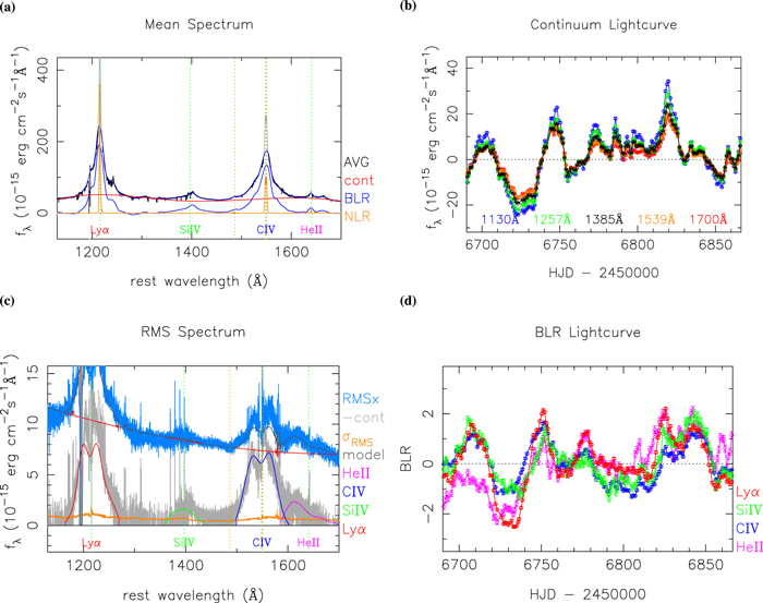
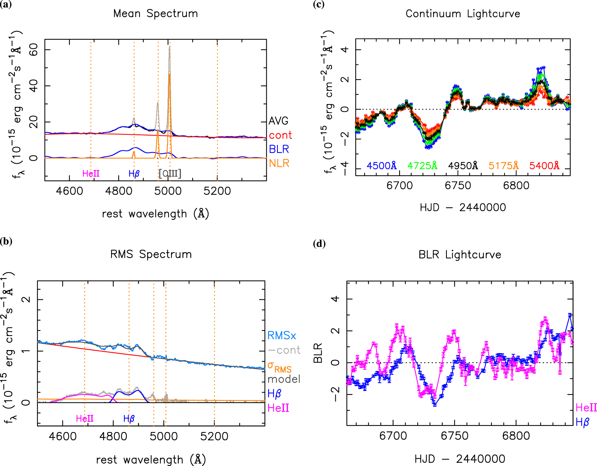
Figure 1. Results of the PrepSpec fit to the HST data. (a) The mean spectrum A(λ) (gray) is decomposed into the continuum  (red), the BLR spectrum
  (blue), and the NLR spectrum N(λ) (orange). (b) The continuum light curves, C(λ, t), evaluated at five wavelengths across the spectrum. The amplitude is larger on the blue end than on the red end of the spectrum. (c) rms spectra before and after subtracting the continuum variations (blue and gray, respectively), and the corresponding uncertainties (yellow). Also shown are rms spectra for the fitted model (black), for the continuum variations C(λ, t) (red), and for individual broad emission lines Bℓ
(λ) (color-coded as indicated). The blue slope of the continuum variations is evident. The strong Lyα and C iv lines have double-peaked profiles in their rms spectra. (d) BLR light curves Lℓ
(t), normalized to a median of 0 and a mean absolute deviation of 0.6745 (to match the MAD of an rms = 1 Gaussian).
(blue), and the NLR spectrum N(λ) (orange). (b) The continuum light curves, C(λ, t), evaluated at five wavelengths across the spectrum. The amplitude is larger on the blue end than on the red end of the spectrum. (c) rms spectra before and after subtracting the continuum variations (blue and gray, respectively), and the corresponding uncertainties (yellow). Also shown are rms spectra for the fitted model (black), for the continuum variations C(λ, t) (red), and for individual broad emission lines Bℓ
(λ) (color-coded as indicated). The blue slope of the continuum variations is evident. The strong Lyα and C iv lines have double-peaked profiles in their rms spectra. (d) BLR light curves Lℓ
(t), normalized to a median of 0 and a mean absolute deviation of 0.6745 (to match the MAD of an rms = 1 Gaussian).
Download figure:
Standard image High-resolution image
Figure 2. Same as in Figure 1, but here showing results of the PrepSpec fit to the MDM data covering the optical spectral region including the broad Hβ and He ii λ4686 and narrow [O iii] emission lines.
Download figure:
Standard image High-resolution imagePrepSpec decomposes the mean spectrum as

where N(λ) is the NLR spectrum,  is the BLR spectrum, and
  is the continuum. These components are modeled as piecewise-cubic spline functions with different degrees of flexibility: stiff for the continuum, more flexible for the BLR, and very loose for the NLR. The emission-line components are forced to vanish outside a range of velocities around the rest wavelength of each line. After some experimentation, we set the emission-line windows to ±1500 km s−1 for the NLR lines, ±10,000 km s−1 for most of the BLR lines, and ±6000 km s−1 for Hβ. This decomposition can be used to measure emission-line strengths, widths, and velocity profiles in the mean spectrum. However, here we use it mainly to isolate the NLR component N(λ), which PrepSpec uses to improve the flux and wavelength calibrations.
PrepSpec models the continuum variations as low-order polynomials in  ,
,

with Nc coefficients Ck (t) that depend on time. Here

interpolates linearly in  from −1 to +1 over the spectral range from λ1 to λ2. We adopt cubic polynomials, Nc
= 4, to represent the continuum variations in the HST spectra over the rest-frame wavelengths 1130–1720 Å and linear polynomials, Nc
= 2, for the optical MDM spectral range 4500–5400 Å. Lower values of Nc
leave evident fit residuals, and higher values do not significantly improve the fit. PrepSpec uses the full spectral range to define continuum variations relative to the mean spectrum, rather than fitting continua to individual spectra using defined relatively line-free continuum windows.
from −1 to +1 over the spectral range from λ1 to λ2. We adopt cubic polynomials, Nc
= 4, to represent the continuum variations in the HST spectra over the rest-frame wavelengths 1130–1720 Å and linear polynomials, Nc
= 2, for the optical MDM spectral range 4500–5400 Å. Lower values of Nc
leave evident fit residuals, and higher values do not significantly improve the fit. PrepSpec uses the full spectral range to define continuum variations relative to the mean spectrum, rather than fitting continua to individual spectra using defined relatively line-free continuum windows.
PrepSpec models the broad emission line variations as

thus representing the variable component of each line ℓ as a fixed line profile Bℓ
(λ) scaled by its light curve Lℓ
(t). The light curves are normalized to  and
and  . This constraint eliminates degeneracies between the model parameters and lets us interpret Bℓ
(λ) as the rms spectrum of the variations in line ℓ. In the same way as for the mean spectrum, the rms line profiles Bℓ
(λ) are modeled as piecewise-cubic spline functions and set to 0 outside the BLR window for that line. This separable model for the line variations assumes that each line has a fixed line profile that varies in strength with time. Residuals to the PrepSpec fit then reveal the evidence for any changes in the line profile. Such changes contain the information we seek on the velocity–delay structure of the reverberating emission-line region and can reveal other interesting phenomena such as the rotating pattern that we discuss in Section 2.4 below.
. This constraint eliminates degeneracies between the model parameters and lets us interpret Bℓ
(λ) as the rms spectrum of the variations in line ℓ. In the same way as for the mean spectrum, the rms line profiles Bℓ
(λ) are modeled as piecewise-cubic spline functions and set to 0 outside the BLR window for that line. This separable model for the line variations assumes that each line has a fixed line profile that varies in strength with time. Residuals to the PrepSpec fit then reveal the evidence for any changes in the line profile. Such changes contain the information we seek on the velocity–delay structure of the reverberating emission-line region and can reveal other interesting phenomena such as the rotating pattern that we discuss in Section 2.4 below.
2.2. UV Spectra from HST
The UV spectra are the same HST spectra discussed and analyzed with cross-correlation methods in Paper I. These spectra exhibit several narrow absorption systems that interfere with our analysis. We used the spectral modeling analysis in Paper VIII to identify wavelength regions affected by narrow absorption features and remove the narrow absorption effects. The fluxes and uncertainties in these regions are divided by the model transmission function, restoring to a good approximation the flux that would have been observed in the absence of the absorption while also expanding the error bars to appropriately reflect the lower number of detected photons.
Similarly, a Lorentzian optical depth profile provided an approximate fit to the broad wings of the geocoronal Lyα absorption. We divided the observed fluxes and their error bars by the model transmission, approximately compensating for the geocoronal Lyα absorption at moderate optical depths. The opaque core of the geocoronal line was beyond repair, and we omit those wavelengths (1214.3–1216.8 Å) from our analysis.
The main results of our PrepSpec fit to the HST spectra are shown in Figure 1, where the left and right columns show the spectral and temporal components of the model, respectively. In Figure 1(a), the mean spectrum A(λ) is decomposed into the NLR spectrum N(λ) (orange), the BLR spectrum  (blue), and the continuum
  (red). The BLR spectrum has very strong, broad Lyα and C iv emission extending to ±10,000 km s−1, with weaker counterparts in Si iv and He ii. As PrepSpec failed to robustly separate Lyα and N v, we opted to model the Lyα+N v blend as a single line. The NLR spectrum is dominated by Lyα and C iv with narrow emission peaks also at N v and He ii. A few narrow absorption features remain uncorrected that will not adversely affect our analysis. Figure 1(b) shows the continuum light curves, C(λ, t), evaluated at five wavelengths across the spectrum. Continuum variations with a median absolute deviation (MAD) of 16% relative to the continuum in the mean spectrum are detected with S/N ≈ 500. The amplitude is larger at 1130 Å on the blue end than at 1700 Å on the red end of the spectrum. Figure 1(c) shows the rms spectra and Figure 1(d) the corresponding BLR light curves. The blue slope of the continuum variations is again evident in the rms spectrum. The BLR variations are detected with high S/N, ∼400 for Lyα, ∼300 for C iv, ∼120 for He ii, and ∼80 for Si iv. The BLR light curves generally resemble those of the continuum, but with time delays and other systematic differences that are distinct for each line. The strong Lyα and C iv lines are single peaked in the mean spectrum but double peaked in the rms spectrum, suggesting that the variations arise from a disk-like BLR. Variations are detected in N v
λ1240 on the red wing of Lyα, in Si iv
λ1393, and in He ii
λ1640.
(red). The BLR spectrum has very strong, broad Lyα and C iv emission extending to ±10,000 km s−1, with weaker counterparts in Si iv and He ii. As PrepSpec failed to robustly separate Lyα and N v, we opted to model the Lyα+N v blend as a single line. The NLR spectrum is dominated by Lyα and C iv with narrow emission peaks also at N v and He ii. A few narrow absorption features remain uncorrected that will not adversely affect our analysis. Figure 1(b) shows the continuum light curves, C(λ, t), evaluated at five wavelengths across the spectrum. Continuum variations with a median absolute deviation (MAD) of 16% relative to the continuum in the mean spectrum are detected with S/N ≈ 500. The amplitude is larger at 1130 Å on the blue end than at 1700 Å on the red end of the spectrum. Figure 1(c) shows the rms spectra and Figure 1(d) the corresponding BLR light curves. The blue slope of the continuum variations is again evident in the rms spectrum. The BLR variations are detected with high S/N, ∼400 for Lyα, ∼300 for C iv, ∼120 for He ii, and ∼80 for Si iv. The BLR light curves generally resemble those of the continuum, but with time delays and other systematic differences that are distinct for each line. The strong Lyα and C iv lines are single peaked in the mean spectrum but double peaked in the rms spectrum, suggesting that the variations arise from a disk-like BLR. Variations are detected in N v
λ1240 on the red wing of Lyα, in Si iv
λ1393, and in He ii
λ1640.
2.3. Optical Spectra from MDM
Optical spectra from the MDM Observatory were presented and analyzed with a cross-correlation analysis in Paper V. Ground-based spectra taken at facilities other than MDM were excluded from this analysis in order to have a consistent and homogeneous data set taken with the same instrument, same spectral resolution, and so on. The ground-based MDM spectra were taken through a 5''-wide slit and extracted with a 15'' aperture, under variable observing conditions. As a result, each spectrum has a slightly different calibration of flux, wavelength, and spectral resolution. While these residual calibration errors are most evident in the regions around narrow emission lines, they contribute to a smaller extent throughout the spectrum.
To compensate for this, the PrepSpec model M(λ, t) includes small adjustments to the calibrations:

Here the calibration-adjusted model is F(λ, t), given by Equation (1), and the small time-dependent adjustments to the calibration are parameterized by p(t) to model imperfect photometry, Δλ(t) for small changes to the wavelength scale, and Δs(t) for small changes in the spectral resolution. PrepSpec models  to ensure that p(t) remains positive. The median of p(t) is set to unity, since typically a minority of the observed spectra are low owing to slit losses and imperfect pointing or variable atmospheric transparency. While PrepSpec can model
  , Δλ(t), and Δs(t) as low-order polynomials of
  , the wavelength dependence of these calibration adjustments was not needed over the relatively short wavelength span of the MDM data analyzed here.
The main results of our PrepSpec analysis of the MDM spectra are shown in Figure 2. This optical spectral region includes the broad Hβ and He ii λ4686 emission lines and narrow [O iii] emission lines. In the mean spectrum, Figure 2(a), Hβ and [O iii] are strong but He ii is very weak. Hβ also has a narrow component. In the rms spectrum, Figure 2(b), the continuum is bluer than in the mean spectrum, the He ii line is much stronger, and the [O iii] line is very weak (if well calibrated, this emission line should not vary at all and thus should not show a signal in the rms spectrum). Note that the profile of broad Hβ is single peaked in the mean but double peaked in the rms spectrum. The continuum and emission-line light curves are shown in Figures 2(c) and (d), respectively. Maxima and minima in the He ii light curve occur a few days earlier than their counterparts in the Hβ light curve.
2.4. Patterns in Residuals to the PrepSpec Fit
Figure 3 presents results of an analysis of the residuals of the PrepSpec fit to the UV HST (left) and optical MDM (right) spectra. The PrepSpec model assumes for each line a fixed line profile that changes in normalization only. The residuals to the PrepSpec fit thus present a visualization of the evidence for variations in the velocity profiles of the emission lines. They also serve as a check on the success of the absorption-line corrections, the calibration adjustments based on the narrow [O iii] emission lines, and the accuracy of the error estimates.

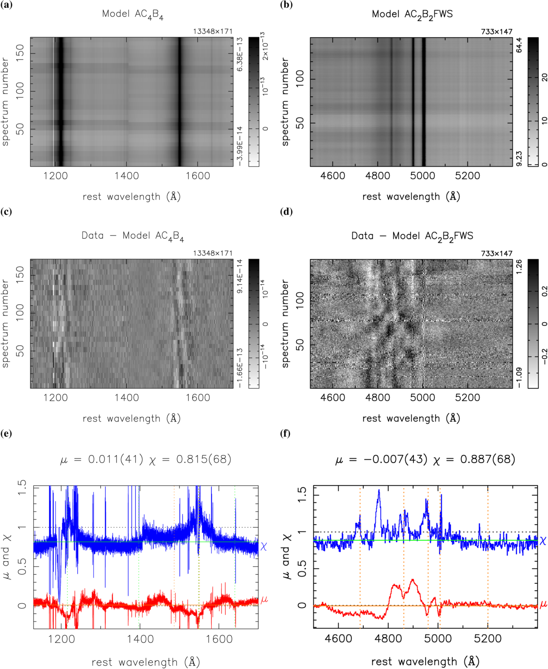
Figure 3. Model (a, b) and residuals (c, d) of the PrepSpec fit to the HST (left) and MDM (right) data. The bottom panels show the mean (red) and rms (blue) over time of the normalized residuals for (e) HST and (f) MDM. Note in panel (c) the helical "Barber-Pole" pattern of stripes moving from red to blue across the C iv and Lyα line profiles. The model specification key includes components A = average spectrum, Cn = continuum polynomial with n parameters, Bn = BLR for n emission lines, and for the MDM data the calibration adjustments F = flux, W = wavelength, and S = seeing.
Download figure:
Standard image High-resolution imageThe top panels, Figures 3(a) and (b), present the fitted PrepSpec model as a grayscale "trailed spectrogram," with wavelength increasing to the right and time upward. Here horizontal bands arise from the continuum variations, and vertical bands mark the locations of emission lines. The middle panels, Figures 3(c) and (d), show residuals after subtracting the PrepSpec model from the observed spectra. There are acceptably small fine-scale residuals near the strong narrow [O iii] lines at 4959 and 5007 Å, indicating the good quality of the calibrations. In Figure 3(d) the evident patterns moving toward the center of the Hβ line arise from reverberations affecting the line wings first and then moving toward the line center. We find below that these can be interpreted as reverberation of Hβ-emitting gas with a Keplerian velocity field. There are also stationary features near 4750, 4880, and 4970 Å that decrease over the 180-day span of the observations, indicating a gradual decrease in the emission-line flux with time.
In Figure 3(c) the dominant residuals near the C iv line exhibit an intriguing helical "Barber-Pole" pattern with stripes moving from red to blue across the line profile. This Barber-Pole pattern may be present also in the Lyα residuals, but less clearly so owing to higher levels of systematic problems created by the absorption-line corrections and blending with N v. We see no clear evidence of the Barber-Pole pattern in the Hβ residuals, where the reverberation signatures are stronger. The peak-to-trough amplitude of these features in C iv is ±8% of the continuum flux density—far too large to be ascribed to calibration errors in the HST spectra.
The bottom panels, Figures 3(e) and (f), show the mean μ(λ) and rms χ(λ) of the normalized residuals, scaled by the error bars. The χ(λ) curves (blue) rise near the emission lines, where significant line profile variations are being detected, and level off in the continuum to values below unity, 0.81 for the HST and 0.89 for the MDM spectra. These low values indicate that rms residuals are smaller than expected from the nominal error bars. For the MEMEcho analysis to follow, we multiply the nominal error bar spectra by these factors.
2.5. Interpretation of the Barber-Pole Pattern
The Barber-Pole pattern is a new phenomenon in AGNs. Manser et al. (2019) report a similar pattern of stripes moving from red to blue across the infrared Ca ii triplet line profiles arising from a thin ring or disk of gas orbiting a white dwarf. The 2 hr period is stable over several years, prompting its interpretation as due to an orbiting planetesimal perturbing the debris disk around the white dwarf.
We tentatively interpret the Barber-Pole pattern in NGC 5548 as evidence for azimuthal structure, perhaps caused by the shadows cast by the vertical structure associated with precessing spiral waves or orbiting material or streamlines near the base of a disk wind, which rotate around the black hole with a period of ∼2 yr. This 2 yr period is estimated based on the impression from Figure 3(c) that the stripes move halfway across the C iv profile during the 180-day campaign, so that 180 days is 1/4 of the period of the rotating pattern. This is clearly just a rough estimate. From the velocity–delay maps discussed in Section 4 below, we infer a black hole mass MBH ≈ 7 × 10⁷
M⊙ and a disk-like BLR geometry extending from 2 to 20 lt-day with an inclination i ≈ 45°. A 2 yr orbital period then occurs at R/c ≈ 4 days, or R ≈ 1000 G
MBH/c2, compatible with the inner region of the BLR. The corresponding Kepler velocity is  km s−1, and this projects to
  km s−1 for i ≈ 45°. These rough estimates are compatible with the observed velocity amplitude of the Barber-Pole stripes in the C iv residuals.
The effect must be stronger on the far side of the disk, to produce Barber-Pole features that move from red to blue across the line profile, and weaker on the near side, where they would be seen moving from blue to red. This front-to-back asymmetry might be due to a bowl-shaped BLR geometry, so that the near side of the BLR disk is strongly foreshortened. However, the velocity–delay maps discussed in Section 4 indicate that the response is stronger on the near side than on the far side of the disk. Alternatively, if the inner disk is tilted toward us, perhaps due to a misaligned black hole spin, then material orbiting there could rise above the outer-disk plane, to cast shadows on the far side of the outer disk, and then dip below the plane to avoid casting shadows on the near side of the outer disk.
Detailed modeling beyond the scope of this paper may test the viability of these and other interpretations. Further monitoring of NGC 5548 with HST may be helpful to determine whether the Barber-Pole phenomenon is stable or transient, whether its period is stable or changing, and whether the stripes always go from red to blue or sometimes from blue to red across the C iv profile.
3. MEMEcho Analysis: Velocity–Delay Mapping
Our echo-mapping analysis is performed with the MEMEcho code, which is described in some detail by Horne (1994). Its ability to recover velocity–delay maps from simulated HST data is demonstrated (Horne et al. 2004), and it has recently been subjected to blind tests (Mangham et al. 2019). We outline below the assumptions and methodology and then present and discuss the results of our MEMEcho analysis of the HST and MDM data on NGC 5548.
Echo mapping assumes that a compact source of ionizing radiation is located at or near the center of the accretion flow. Photons emitted here shine out into the surrounding region, causing local heating and ionization of gas, which then emits a spectrum characterized by emission lines as it cools and recombines. Reprocessing times are expected to be short and dynamical times long compared to light-travel times. As distant observers, we see the response from each reprocessing site with a time delay τ from the light-travel time and a Doppler shift v from the line-of-sight velocity. Thus, the reverberating emission-line spectrum encodes information about the geometry, kinematics, and ionization structure of the accretion flow—to be more specific, that part of the flow that emits the reverberating emission lines.
To decode this information, we interpret the observed spectral variations as time-delayed responses to a driving light curve. By fitting a model to the reverberating spectrum F(λ, t), we reconstruct a two-dimensional wavelength–delay map Ψ(λ, τ). This effectively slices up the accretion flow on isodelay surfaces, which are paraboloids coaxial with the line of sight with a focus at the compact source. Each delay slice gives the spectrum of the response, revealing the fluxes and Doppler profiles of emission lines from gas located on the corresponding isodelay paraboloid. The resulting velocity–delay maps Ψ(v, τ) provide two-dimensional images of the accretion flow, one for each emission line, resolved on isodelay and isovelocity surfaces.
3.1. Linearized Echo Model
The full spectrum of ionizing radiation is not observable, and so an observed continuum light curve, C(t), is adopted as a proxy. At each time delay τ, the responding emission-line light curve L(t) is then some nonlinear function of the continuum light curve C(t − τ) shifted to the earlier time t − τ. In addition, the observed line and continuum fluxes include constant or slowly varying background contributions from other light sources, such as narrow-line emission and starlight from the host galaxy. To model these backgrounds and account for the nonlinear BLR responses, MEMEcho employs a linearized echo model, with reference levels C0 for the continuum and L0 for the line flux, and a tangent-curve approximation to variations around these reference levels. Thus, the continuum light curve C(t) is decomposed as

and the emission-line light curve,

is a convolution of the continuum variations with a delay map Ψ(τ), giving the one-dimensional delay distribution of the emission-line response. We find that this linearized echo model fails to provide a good fit to the NGC 5548 data. We therefore generalize the model to allow a time-dependent echo background level, L0(t). This extension is straightforward .
3.2. Maximum Entropy Regularization
Maximum entropy regularization keeps the model light curves C(t) and L0(t) and the delay maps Ψ(τ) positive and "as smooth as possible" while fitting the data. Referring to these functions generically as p(t), the entropy is

measured with weights w(t) and relative to a default function q(t). We obtain q(t) by Gaussian smoothing of p(t), with an FWHM of 1, 2, and 4 days for the driving light curve, the delay map, and the echo background, respectively. These choices control the flexibility of the functions. The weights w(t) provide additional control on relative flexibility among the three functions.
For fits to reverberating spectra, the MEMEcho model simply adds a wavelength dimension to the echo light curve, L(t) → L(λ, t), to the response distribution, Ψ(τ) → Ψ(λ, τ), and to the background variations, L0(t) → L0(λ, t). These two-dimensional functions are then regularized with the entropy defined relative to default functions that average in both directions.
The MEMEcho fit is accomplished by iteratively adjusting the functions p to minimize

Here  quantifies the "badness of fit" to the N data D, assuming Gaussian noise with known error bars. The Lagrange multiplier α controls the trade-off between fitting the data (small χ2) and being simple (large S). In practice, α is initially large, and a series of converged fits is constructed with decreasing χ2 and increasing S, stopping when the fit is judged to be satisfactory (χ2/N ≈ 1) and the model not overly complex.
3.3. Delay Maps Ψ(τ) for NGC 5548
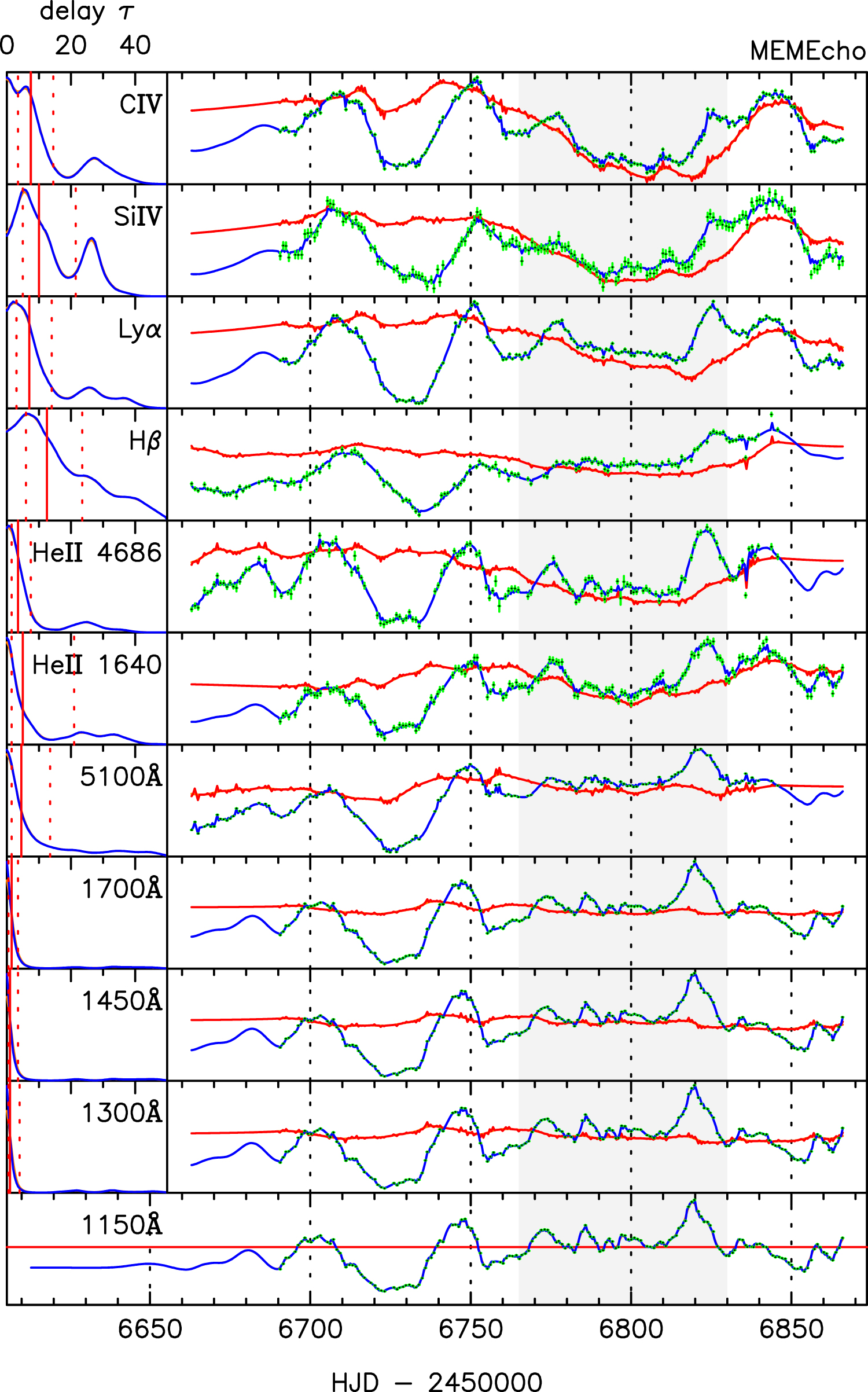
Figure 4 shows the results of our MEMEcho fit to five continuum and six emission-line light curves of NGC 5548. The light-curve data are from the PrepSpec analysis of the HST and MDM spectra, described in Section 2. MEMEcho fits all light curves simultaneously, recovering a model for the driving light curve C(t), and for each echo light curve a delay map Ψ(τ) and a background light curve L0(t). The driving light curve C(t) (bottom panel of Figure 4) is the 1150 Å continuum light curve, with the reference level C0 (red line) set at the median of the 1150 Å continuum data. Above this are 10 echo light curves (right) and corresponding delay maps (left), where the light-curve data (black points with green error bars) can be directly compared with the fitted model (blue curves). We model four continuum light curves, at 1300, 1450, and 1700 Å from the HST spectra and at 5100 Å from the MDM spectra, as echoes of the 1150 Å continuum. The reverberating emission lines are He ii λ1640 and He ii λ4686, then Hβ and Lyα, and finally Si iv and C iv. The MEMEcho fit accounts for much of the light-curve structure as echoes of the driving light curve but requires significant additional variations L0(t) (red curves), particularly during the BLR Holiday indicated by gray shading in Figure 4.
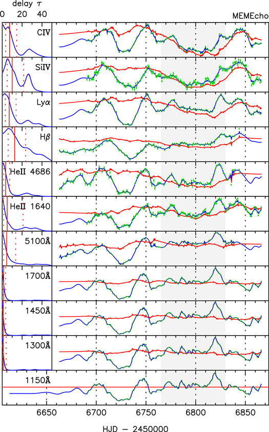
Figure 4. MEMEcho fits to five continuum and six emission-line light curves of NGC 5548. The driving light curve (bottom panel) is the 1150 Å continuum light curve with a reference level (red line) at the median of the 1150 Å continuum data. Above this are 10 echo light curves (right) and corresponding delay maps (left), comparing the light-curve data (the black points with green error bars) and the echo model (blue curves) with slow background variations (red curves). The echoes (bottom up) are four continuum light curves, at 1300, 1450, and 1700 Å from the HST spectra and at 5100 Å from the MDM spectra, then six reverberating emission lines (He ii λλ1640, 4686, Hβ, Lyα, Si iv, and C iv). On each delay map in the left column, the median delay is marked by a vertical line, flanked by vertical dashed lines for the quartiles of the delay distribution. The MEMEcho fit accounts for much of the light-curve structure as echoes of the driving light curve but requires significant additional variations (red curves). The gray shaded region indicates the time span of the "BLR Holiday" identified in Paper IV.
Download figure:
Standard image High-resolution imageThe fit shown in Figure 4 requires χ2/N = 1 separately for the driving light curve and for each of the echo light curves, where there are N = 171 and 147 data points for the HST and MDM light curves, respectively. The model light curves (delay maps) are evaluated on a uniform grid of times (delays) spaced by Δt = 0.5 days, linearly interpolated to the times of the observations. The delay maps span a delay range of 0–50 days.
The delay maps Ψ(τ) are of primary interest because they indicate the radial distributions from the central black hole over which the continuum and emission lines are responding to variations in the driving radiation. The continuum light curves exhibit highly correlated variations that are well fit by exponential delay distributions strongly peaked at τ = 0. The median delay, increasing with wavelength, is ∼1 day at 1700 Å and ∼5 days at 5100 Å. The echo background has only small variations, indicating that the linearized echo model is a very good approximation for the continuum light curves.
The emission-line light curves require more extended delay distributions and larger variations in their background levels. The background variations are similar, but not identical, for the six emission-line light curves. The two He ii light curves require tight delay distributions peaking at τ = 0, with half the response inside ∼5 days and 3/4 inside 10 days, and some low-level structure at 20–40 days. The background light curves have a "slow wave" with a 100-day timescale, somewhat different for the two lines, and smaller-amplitude 10-day structure. The slow-wave background for He ii λ1640 is rising from HJD 6690 to 6750 (really HJD−2,450,000), while that for He ii λ4686 is more constant. Both backgrounds then decline to minima around HJD 6800 and then rise until 6840. The constant background for He ii λ1640 prior to HJD 6690 and for He ii λ4686 after HJD 6850 is not significant since there are no data during these intervals.
The Hβ response exhibits the most extended delay distribution, with a peak at 7 days, half the response inside 14 days, 3/4 inside 23 days, minor bumps at 25 and 40 days, and falling to 0 at 50 days. The need for this extended delay map is evident in the Hβ light curve, for example, to explain the slow Hβ decline following peaks at HJD 6705 and 6745. The Lyα response is more confined than Hβ with a peak at 3 days, half the response inside 7 days, 3/4 inside 15 days, and bumps at 26 and 35 days. Si iv and C iv are similar, with peaks at 5 and 7 days, respectively.
The slow-wave backgrounds L0(t) for all these lines fall slowly from HJD 6740 to 6820 and then rise more rapidly to a peak at HJD 6840. This corresponds approximately to the anomalous BLR Holiday period discussed in Paper IV, indicated by gray shading in Figure 4, during which the emission lines became weak relative to the continuum. Note also a smaller dip from HJD 6715 to 6740 that serves to deepen the emission-line decline between the two peaks, particularly for C iv. A small peak near HJD 6810 accounts for emission-line peaks in C iv, Si iv, and He ii λ1640 that have no clear counterpart in the continuum light curves.
Note that the model and background light curves (blue and red curves in Figure 4) exhibit numerous small spikes in addition to smoother 100-day and 10-day structure. These spikes correspond to data points that are too high or too low, relative to their error bars, to be fit by the smooth default light curve that maximizes the entropy. The largest offender is a low point in the Hβ and He ii λ4686 light curves near HJD 6837, which likely represents a calibration error. These outliers could seriously damage the delay maps. The spikes are less prominent if we relax the fit to a higher χ2/N, but then the fit to the relatively low S/N Si iv light curve is less satisfactory. Fortunately, because our model has time-dependent backgrounds that can develop sharp spikes where required, the delay maps remain relatively smooth and insensitive to these outliers.
4. Velocity–Delay Maps
Velocity–delay maps project the information that is coded in the reverberating emission-line profile onto a two-dimensional map of the six-dimensional position–velocity phase space of the BLR gas. While this is incomplete information, an ordered velocity field can have an easily recognizable signature in the velocity–delay map; some examples are shown by Welsh & Horne (1991). A signature of inflowing gas is short delays on the red wing of the velocity profile and a wide range of delays on the blue side. Outflowing gas has a similar but reversed signature. An orbiting ring of gas at radius R maps into an ellipse on the velocity–delay plane, centered at τ = R/c and extending over  , allowing the identification of R and i. A Keplerian disk superimposes these ellipses to form a "virial envelope" that can be used to infer
  at each R. Assuming
  , this gives
  . Thus, a sufficiently crisp velocity–delay map can be read to infer the general nature of the flow in the BLR, and several specific parameters of the geometry and kinematics. With velocity–delay maps for several lines, the radial ionization structure in the BLR becomes manifest, and subtle structures such as spiral density waves may become evident (Horne et al. 2004). Constructing velocity–delay maps was therefore the principal motivation for undertaking the STORM campaign.
4.1. MEMEcho Fits to the Spectral Variations
Wavelength–delay maps Ψ(λ, τ) of the emission-line response in NGC 5548 are shown as two-dimensional false-color images in Figure 5 for the MEMEcho fit to the optical spectra from MDM and in Figure 6 for the UV spectra from HST.
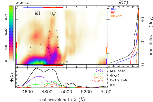
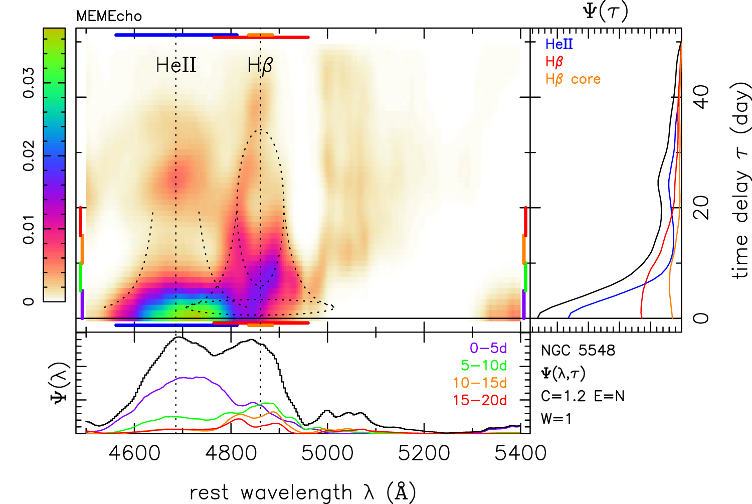
Figure 5. Two-dimensional wavelength–delay map Ψ(λ, τ) reconstructed from the MEMEcho fit to the optical spectra from MDM. Delays are measured relative to the 1150 Å continuum light curve. Panels below and to the right of the map give the projected responses Ψ(λ) and Ψ(τ). Here the black curve is the full response, and the colored curves are for the wavelength or delay ranges indicated by the correspondingly colored bars in the margins of the map. Dotted curves show the envelope around each line inside which emission can occur from a Keplerian disk inclined by i = 45° orbiting a black hole of mass MBH = 7 × 10⁷ M⊙. The ellipses shown for Hβ correspond to Keplerian disk orbits at R = 2 and 20 lt-day. The units of Ψ(λ, τ), indicated on the color bar, are 1/day.
Download figure:
Standard image High-resolution image
Figure 6. Same as in Figure 5, but showing the two-dimensional wavelength–delay map Ψ(λ, τ) reconstructed from the MEMEcho fit to the UV spectra from HST. The ellipses shown for Lyα and C iv correspond to Keplerian disk orbits at R = 2 and 20 lt-day.
Download figure:
Standard image High-resolution imageIn the panel to the right of the 2D map, the projections Ψ(τ) give delay maps for the full wavelength range (black) and for velocity ranges centered on the rest wavelengths of the emission lines, as indicated by the colored bars above and below the map. In the panel below, the projections Ψ(λ) give the spectrum of the full response (black) and of the response in four delay ranges, 0–5 days (purple), 5–10 days (green), 10–15 days (orange), and 15–20 days (red). Velocity–delay maps centered on the six emission lines are presented in Figure 7. These two-dimensional maps show that the emission-line response inhabits the interior of a virial envelope (dashed) and exhibit structure indicating a Keplerian disk inclined by i = 45° and with an outer rim at R/c = 20 days, as discussed below. These maps and their interpretation are the main results of interest emerging from our MEMEcho analysis.

Figure 7. Velocity–delay maps Ψ(v, τ) reconstructed from the MEMEcho fit to the HST and MDM spectra. Delays are measured relative to the 1150 Å continuum light curve. Velocities are measured relative to the rest wavelength of the indicated line. Dashed black curves show the virial envelope around each line inside which emission can occur from a Keplerian disk inclined by i = 45° orbiting a black hole of mass MBH = 7 × 10⁷ M⊙. The dashed ellipse corresponds to a circular Keplerian orbit at the outer-disk rim radius R/c = 20 days. Note that the red wing of Lyα is blended with N v and the blue wing of Hβ is blended with He ii λ4686. A scale bar corresponding to 10 μas is shown in each panel.
Download figure:
Standard image High-resolution imageDetails from the MEMEcho fit are shown in Figures 8 and 9 for the HST and MDM spectra, respectively, with the same format as in Figure 4. The fit models as echoes the same four continuum light curves (at 1350, 1450, 1700, and 5100 Å), and now as well the continuum-subtracted emission-line variations across the full wavelength range of the HST and MDM spectra. The PrepSpec model provided the variable continuum model that was subtracted to isolate the BLR spectra used in the MEMEcho fit. As before, the proxy driving light curve C(t) is the continuum light curve at 1150 Å. The model allows echo responses over a delay range of 0–50 days and includes a time-variable background spectrum L0(λ, t). This allows the model to account for the period of anomalous line response during the BLR Holiday (Paper IV) and any other features in the data, real or spurious, that are not easily interpretable in terms of the linearized echo model. Figure 10 presents a grayscale "trailed spectrogram" display of the slowly varying background L0(λ, t) for the MEMEcho fit to the HST and MDM spectra. The Barber-Pole pattern of residuals and the BLR Holiday features are evident here.
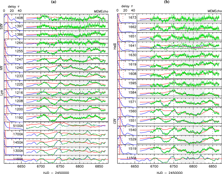
Figure 8. Details of the MEMEcho fit to the spectral variations in the HST data. Gray shading indicates the dates of the BLR Holiday. The light-curve data (black dots) with error bars (green) are compared with the fitted model (blue) and varying background (red). This global fit to N = 125,448 data points achieved a reduced χ2/N = 1.2. The bottom panel shows the driving light curve at 1150 Å. Above this are delay maps (left) and echo light curves (right). (a) Continuum echoes at 1300, 1450, 1700, and 5100 Å, and the continuum-subtracted emission at selected wavelengths, including Lyα λ1216, N v λ1240, and Si iv λ1393. (b) Echo maps and light curves for selected wavelengths, including C iv λ1549 and He ii λ1640.
Download figure:
Standard image High-resolution image
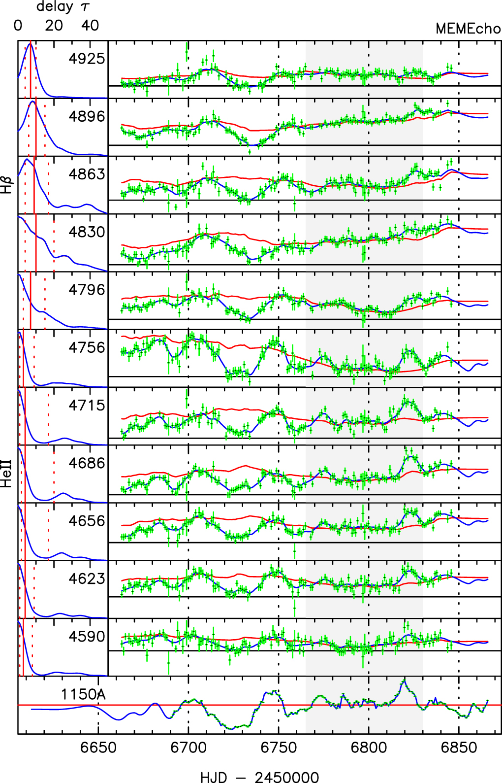
Figure 9. Details of the MEMEcho fit to the spectral variations in the MDM data. Gray shading indicates the dates of the BLR Holiday. The light-curve data (black dots) with error bars (green) are compared with the fitted model (blue) and the varying background (red). This global fit to N = 125,448 data points achieved a reduced χ2/N = 1.2. The bottom panel shows the driving light curve at 1150 Å. Above this are delay maps (left) and echo light curves (right) for continuum echoes at 1300, 1450, 1700, and 5100 Å, and for continuum-subtracted emission at selected wavelengths, including He ii λ1640 and Hβ λ4861.
Download figure:
Standard image High-resolution image
Figure 10. Slowly varying background component  of the MEMEcho model fitted to the HST data (left) and MDM data (right). The model's time-averaged spectrum has been subtracted to leave time-varying residuals. The right panels show the wavelength-averaged response, with gray shading indicating the BLR Holiday dates. The bottom panels show the mean (blue) and rms (red) of the time-dependent residuals at each wavelength. All lines show a depressed flux during the BLR Holiday. The helical Barber-Pole pattern, with stripes moving from red to blue across the line profile, is evident in the C iv and Lyα residuals. The Barber-Pole pattern is absent in He ii and may be present in Hβ but with a less clear pattern.
Download figure:
Standard image High-resolution image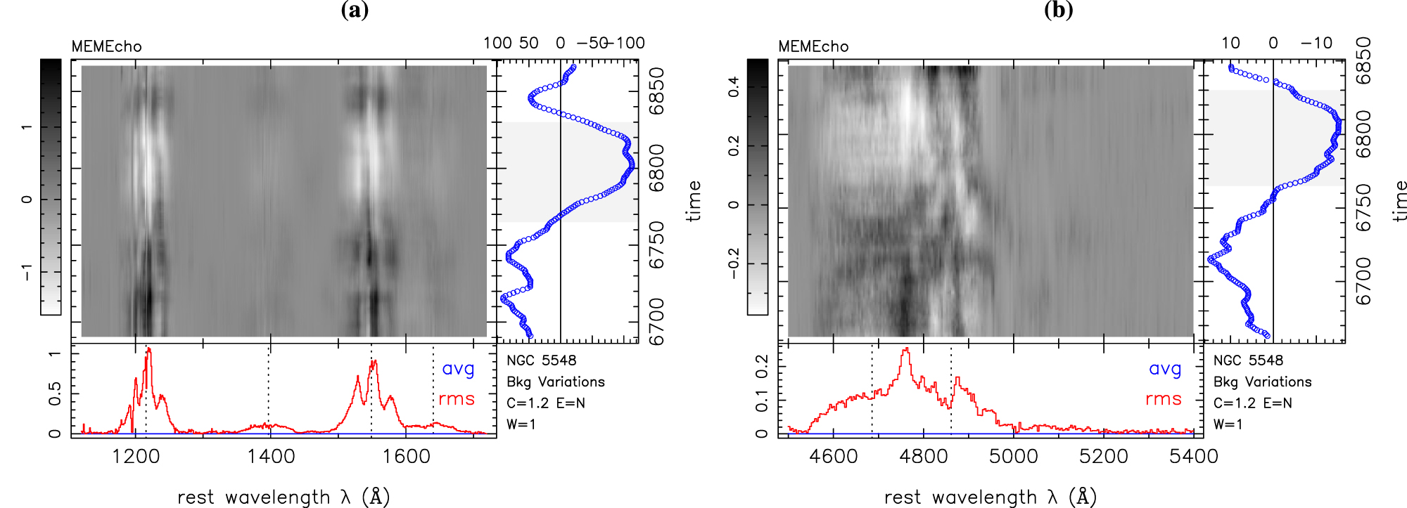
To regularize these fits, which include two-dimensional wavelength–delay maps Ψ(λ, τ) and varying background spectra L0(λ, t), the entropy now steers the fit toward models with smooth spectra, as well as smooth light curves and delay maps. We actually construct a series of MEMEcho maps that fit the data at different values of χ2/N, ranging from 5 to 1. At higher χ2, the fit to the data is poor and the maps are smooth. At lower χ2, the fit improves and the maps develop more detailed structure. When χ2 is too low, the fit becomes strained as the model strives to fit noise features (e.g., by introducing spikes in the gaps between data points in the driving light curve). The fits and maps shown here for a fit with χ2/N = 1.2 are a good compromise between noise and resolution. Our tests show that the main features interpreted here are robust to changes in the control parameters of the fit. These parameters adjust the relative "stiffness" of the driving light curve, the background light curve, the echo maps, and the aspect ratio of resolution in the velocity and delay directions.
4.2. Interpretation of the MEMEcho Maps
From Figures 5 and 6, the three strongest lines—Lyα, C iv, and Hβ—have a similar velocity–delay structure, with most of their response occurring between 5 and 15 days. To first order, the response in all three lines is red–blue symmetric. This indicates that radial motions are subdominant in the BLR, as a strong inflow (outflow) component would produce shorter delays on the red (blue) side of the velocity profile (Welsh & Horne 1991).
The He ii response is largely inside 5 days and extends to ±10,000 km s−1, compatible with expected radial ionization structure and virial motions. In Figure 5, we see that He ii response is broad and single peaked. He ii dominates the Hβ response in the delay slice of 0–5 days (purple), becomes subdominant at 5–10 days (green), and is almost negligible at larger delays. The He ii λ1640 and He ii λ4686 delay ranges and velocity structures are similar. There is no signature of a double-peaked structure in these two lines.
In Figure 5, the Hβ delay maps Ψ(τ) for the full profile (±6000 km s−1; red) and for the line core (±1500 km s−1; orange) are flat or rising from 0 to 10 days and then tail away. The Hβ response spectrum Ψ(λ) exhibits a double-peaked structure in the delay ranges of 10–15 days (orange) and 15–20 days (red), with the peaks separated by ∼5000 km s−1. In the slice of 5–10 days, the Hβ response has a central peak flanked by ledges that extend to ±5000 km s−1. Figure 6 shows similar double-peaked responses in Lyα and somewhat less clearly in C iv.
Clearly recognizable in the velocity–delay structure is the signature of an inclined Keplerian disk with a well-defined outer edge. The velocity–delay maps provide a plausible interpretation for the "M"-shaped variation in lag with velocity seen in the cross-correlation results (Papers I and V). The outer edges of the "M" arise from the virial envelope. The "U"-shaped interior of the "M" dips down from 20 to 5 days, and we interpret this as the lower half of an ellipse in the velocity–delay plane, which is the signature of a ring of gas orbiting the black hole at radius R = 20 lt-day.
The Hβ response exhibits the clearest signature of an ellipse in the velocity–delay plane, corresponding to an annulus in the Keplerian disk. The (stronger) near side of the annulus has a delay at  days, and the (weaker) far side extends to
  days. Assuming a thin disk, the ratio gives
  , or i ≈ 45°. The double-peaked velocity structure at τ ≈ 20 days then gives the black hole mass. The framework shown by dashed orange curves on Figures 8 and 9 was adjusted by eye to fit the main features. This provides rough estimates for the black hole mass MBH ≈ 7 × 10⁷
M⊙, the inclination i ≈ 45°, and the outer BLR radius Rout ≈ 20 lt-day. Note that the characteristic BLR response timescale, as measured by the mode or mean or median of Ψ(τ), is less than R/c at the outer edge of the BLR.
, or i ≈ 45°. The double-peaked velocity structure at τ ≈ 20 days then gives the black hole mass. The framework shown by dashed orange curves on Figures 8 and 9 was adjusted by eye to fit the main features. This provides rough estimates for the black hole mass MBH ≈ 7 × 10⁷
M⊙, the inclination i ≈ 45°, and the outer BLR radius Rout ≈ 20 lt-day. Note that the characteristic BLR response timescale, as measured by the mode or mean or median of Ψ(τ), is less than R/c at the outer edge of the BLR.
The velocity–delay structure also indicates a stronger response from the near side than from the far side of the inclined disk. We see the upper half of the ellipse only faintly in the velocity–delay map of Hβ and perhaps also for Lyα. The C iv map and the (less reliable) Si iv map show a faint response at 25–30 days that is not very clearly connected to the stronger response inside 10–15 days. If the response structure were azimuthally symmetric, the upper and lower halves of the ellipse would be more equally visible. The mean delay averaged around the ellipse would be R/c ≈ 20 days, and this is similar to typical Hβ lags seen in the past. The much shorter lags in the STORM data may be interpreted as due at least in part to an anisotropy present in 2014 that was usually much weaker or absent during previous monitoring campaigns. The near/far contrast ratio can be determined by more careful modeling.
5. Discussion
5.1. Parameter Uncertainties
The morphology of the velocity–delay maps indicates that the BLR in NGC 5548 is compatible with a disk-like geometry and kinematics, for a black hole mass MBH ≈ 7 × 10⁷ M⊙, an inclination angle i ≈ 45°, and a relatively sharp outer rim at R/c ≈ 20 days. Uncertainties in these parameters are difficult to quantify precisely because MEMEcho delivers the "smoothest positive" maps that fit the data at specified levels of χ2/N. This relatively model-independent approach does not aim to determine model-specific parameters. However, by comparing the velocity–delay maps with those of toy models, we estimate that MBH is uncertain by ∼20%, the inclination by ∼ 10°, and R/c by ∼10%.
Future and ongoing efforts to model the STORM data will incorporate more specific geometric and kinematic parameters and photoionization physics. These should allow for parameter estimates with better-quantified uncertainties. At this stage the value of the velocity–delay maps is to inform the dynamical modeling efforts by indicating what types of models are likely to succeed.
5.2. Comparison with 2008 Mass Estimates
NGC 5548 was one of 13 AGNs monitored during the Lick AGN Monitoring Project (LAMP) 2008 RM campaign (Bentz et al. 2009; Walsh et al. 2009). Using spectra from the 3 m Shane telescope at Lick Observatory and Johnson V and B broadband photometry from a number of ground-based telescopes, the LAMP 2008 campaign secured 57 V-band continuum and 51 Hβ line epochs on NGC 5548 over a 70-day span. The centroid Hβ lag measured by cross-correlation methods is  days. Combined with the Hβ line width σline = 4270 ± 290 km s−1 from the rms spectrum, the virial product is
  M⊙, giving the black hole mass as
  M⊙, where f is the adopted calibration factor, uncertain by ∼0.3 dex for individual AGNs.
Pancoast et al. (2014) present results of a dynamical modeling fit to the 2008 LAMP data on NGC 5548. The caramel code employs Markov Chain Monte Carlo methods to sample the parameters of a dynamical model of the Hβ-emitting region. Taking the V-band data as a proxy for the driving light curve, caramel fits the reverberating emission-line profile variations by adjusting the spatial and kinematic distribution of Hβ-emitting clouds. This model incorporates more detailed model-specific information than the MEMEcho mapping but is flexible enough to explore a variety of inflow and outflow as well as disk-like kinematic structures. The caramel fit to NGC 5548 in 2008 finds a mean delay of just 3 days, indicating a smaller Hβ emission-line region. The caramel model fitted to the 2008 data has a thick-disk geometry, with an opening angle  , a dominant Hβ response on the far side of the disk, and a strong inflow signature, with small delays on the red wing relative to those on the blue wing of Hβ. The inflow and far-side response in 2008 are quite different from the symmetric disk-like kinematics and near-side response evident in the MEMEcho velocity–delay maps. Despite these differences and the smaller size of the Hβ emission-line region in 2008, the inferred mass
  M⊙ and inclination
  are consistent, given their uncertainties, with the corresponding values, MBH ≈ 7 × 10⁷
M⊙ and i ≈ 45°, that we estimate from the structure of the Hβ velocity–delay maps from the 2014 STORM data. The mass estimate from the caramel fit may be too small owing to the Hβ response being measured relative to the optical continuum, which itself may have a delay of a few days. For example, in 2014 the V-band delay was 1.6 ± 0.5 days (Paper II), and that could boost the caramel mass estimate by ∼50%, bringing it into closer agreement with our estimate from the velocity–delay maps.
are consistent, given their uncertainties, with the corresponding values, MBH ≈ 7 × 10⁷
M⊙ and i ≈ 45°, that we estimate from the structure of the Hβ velocity–delay maps from the 2014 STORM data. The mass estimate from the caramel fit may be too small owing to the Hβ response being measured relative to the optical continuum, which itself may have a delay of a few days. For example, in 2014 the V-band delay was 1.6 ± 0.5 days (Paper II), and that could boost the caramel mass estimate by ∼50%, bringing it into closer agreement with our estimate from the velocity–delay maps.
5.3. Comparison with 2015 Velocity–Delay Maps
During 2015 January–July, a year after the STORM campaign, NGC 5548 was monitored with the Yunnan Faint Object Spectrograph and Camera on the 2.4 m telescope at Lijiang, China, resulting in 61 good spectra over 205 days that provide the basis for an MEM analysis yielding a velocity–delay map for Hβ (Xiao et al. 2018). This 2015 map exhibits structure remarkably similar to that seen in our 2014 map, including the virial envelope, the "M"-shaped structure with τ ≈ 10 days and V ≈ ± 2400 km s−1 at the peaks of the "M," and a well-defined ellipse extending out to τ ≈ 40 days.
Xiao et al. (2018) also present Hβ velocity–delay maps constructed from 13 annual AGNWatch campaigns during 1989–2001. While several of these maps show hints of a ring-like structure, the quality of these maps is much lower owing to less intensive time sampling, making it difficult to be confident about the information that they may be able to convey.
In combination, the high-fidelity 2014 and 2015 Hβ velocity–delay maps each show a clear virial envelope and distinct ellipse centered at 20 lt-day. Thus, at both epochs the Hβ response arises from a Keplerian disk with a relatively sharp outer rim at 20 lt-day that remained stable for an interval of at least a year. In 2014 the response is weak on the top of the velocity–delay ellipse. In 2015 the response is clearly visible on the blue side and over the top of the velocity–delay ellipse and relatively weak on the red side. This indicates significant azimuthal modulation of the response that evolves, perhaps rotates, on a timescale of a year. Future velocity–delay mapping experiments to monitor this structure could be interesting to elucidate its origin and implications.
5.4. Barber-Pole Patterns
The Barber-Pole pattern uncovered here in NGC 5548 may be related to intermittent periodic phenomena seen in the subclass of AGNs that have double-peaked Balmer emission lines. In these double-peaked emitters there is a clear separation between the narrow emission lines and the broad double-peaked lines. The double-peaked velocity profiles can be modeled by emission from a Keplerian disk, with relativistic effects making the blue peak stronger and sharper than the red one and redshifting the line center. Spectroscopic monitoring of Arp 102B during 1987–1996 detected Hβ profile variations (Newman et al. 1997). In particular, during 1991–1995, the Hβ red/blue flux ratio oscillates over nearly 2 cycles of a 2.2 yr period, suggesting a patch of enhanced emission on a circular orbit within the disk. Contemporaneous monitoring of Hα during 1992–1996 shows that its red/blue flux ratio also oscillates by ±10% with a 2 yr period (Sergeev et al. 2000). A trailed spectrogram display of the Hα residuals, after subtracting scaled mean line profiles, reveals a helical Barber-Pole pattern with two stripes that move from red to blue across the double-peaked Hα profile. This is strikingly similar to what we see in the C iv profile of NGC 5548. Similar phenomena are seen in other double-peaked emitters (Gezari et al. 2007; Lewis et al. 2010; Schimoia et al. 2015, 2017). Our discovery of the Barber-Pole pattern in NGC 5548 indicates that this phenomenon is not limited to the double-peaked emitters.
6. Summary
In this paper, we achieve the primary goal of the AGN STORM campaign by recovering velocity–delay maps for the prominent, broad, Lyα, C iv, He ii, and Hβ emission lines in NGC 5548. These are the most detailed velocity–delay maps yet obtained for an AGN, providing unprecedented information on the geometry, ionization structure, and kinematics of the broad-line region.
Our analysis interprets the ultraviolet HST spectra (Paper I) and optical MDM spectra (Paper V) secured in 2014 during the 6-month STORM campaign on NGC 5548. This data set provides spectrophotometric monitoring of NGC 5548 with unprecedented duration, cadence, and S/N suitable for interpretation in terms of reverberations in the BLRs surrounding the black hole. Assuming that the time delays arise from light-travel time, the velocity–delay maps we construct from the reverberating spectra provide two-dimensional projected images of the BLR, one for each line, resolved on isodelay paraboloids and line-of-sight velocity.
We used the absorption-line modeling results from Paper VIII to divide out absorption lines affecting the HST spectra. We used PrepSpec to recalibrate the flux, wavelength, and spectral resolution of the optical MDM spectra using the strong narrow emission lines as internal calibrators. Residuals from the PrepSpec fits indicate the success of the calibration adjustments.
The linearized echo model that we normally use for echo mapping is violated in the STORM data set by anomalous emission-line behavior, the BLR Holiday discussed in Paper IV. We model this adequately as a slowly varying background spectrum superimposed on which are the more rapid variations due to reverberations.
The residuals of the PrepSpec fits reveal significant emission-line profile changes. Features are evident moving inward from both red and blue wings toward the center of the Hβ line, interpretable as reverberations of a BLR with a Keplerian velocity field.
A helical "Barber-Pole" pattern with stripes moving from red to blue across line profile is evident in the C iv and possibly also the Lyα lines, suggesting an azimuthal structure rotating with a period of ∼2 yr around the far side of the accretion disk. This may be due to precession or orbital motion of disk structures. Similar behavior is seen in the double-peaked emitters, such as Arp 102B. Further HST observations of NGC 5548 over a multiyear time span, with a cadence of perhaps 10 days rather than 1 day, could be an efficient way to explore the persistence, transience, and nature of this new phenomenon in NGC 5548.
We use the PrepSpec fit to extract light curves for the lines and continua and use MEMEcho to fit these light curves using the 1150 Å continuum light curve as a proxy for the driving light curve. The MEMEcho fit determines a set of echo maps Ψ(τ) giving the delay distribution of each echo, effectively slicing up the reverberating region on isodelay paraboloids. The structure in these echo maps indicates radial stratification, with He ii responding from inside 5 lt-day and the Lyα C iv, and Hβ response extending out to or beyond 20 lt-day.
By using MEMEcho to fit reverberations in the emission-line profiles, we construct velocity–delay maps Ψ(v, τ) that resolve the BLR in time delay and line-of-sight velocity. The BLR response is confined within a virial envelope around each line, with double-peaked velocity profiles in the response in delay slices of 10–20 days. The "M"-shaped changes in delay with velocity, found using velocity-resolved cross-correlation lags in Papers I and V, are seen here to be the signature of a Keplerian disk. The outer legs of the "M" arise from the virial envelope between 5 and 20 days; the inner "U" of the "M" is the lower part of an ellipse extending from 5 to 35 days. This velocity–delay structure is most straightforwardly interpreted as arising from a Keplerian disk extending from R/c = 5 to 20 days, inclined by i ≈ 45°, and centered on a black hole of mass MBH ≈ 7 × 10⁷ M⊙. The BLR has a well-defined outer rim at R/c ≈ 20 days, but the far side of the rim may be obscured or less responsive than the near side.
Detailed modeling of the STORM data, guided by the features in the velocity–delay maps presented here, should be able to refine and quantify uncertainties on these features of the BLR, the inclination, and the black hole mass.
Support for HST program No. GO-13330 was provided by NASA through a grant from the Space Telescope Science Institute, which is operated by the Association of Universities for Research in Astronomy, Inc., under NASA contract NAS5-26555. K.H. acknowledges support from STFC grant ST/R000824/1. G.D.R., B.M.P., M.M.F, C.J.G., and R.W.P. are grateful for the support of the National Science Foundation (NSF) through grant AST-1008882 to The Ohio State University. Research at UC Irvine has been supported by NSF grants AST-1412693 and AST-1907290. M.C. Bentz gratefully acknowledges support through NSF CAREER grant AST-1253702 to Georgia State University. V.N.B. gratefully acknowledges assistance from National Science Foundation (NSF) Research at Undergraduate Institutions (RUI) grant AST-1909297. S.B. is supported by NASA through Chandra award AR7-18013X issued by the Chandra X-ray Observatory Center, operated by the Smithsonian Astrophysical Observatory for and on behalf of NASA under contract NAS8-03060. S.B. was also partially supported by grant HST-AR-13240.009. M.C. Bottorff acknowledges HHMI for support through an undergraduate science education grant to Southwestern University. E.M.C., E.D.B., L.M., and A.P. acknowledge support from Padua University through grants DOR1699945/16, DOR1715817/17, DOR1885254/18, and BIRD164402/16. G.F. and M. Dehghanian acknowledge support from the NSF (AST-1816537), NASA (ATP 17-0141), and STScI (HST-AR-13914, HST-AR-15018), and the Huffaker Scholarship. K.D.D. is supported by an NSF Fellowship awarded under grant AST-1302093. R.E. gratefully acknowledges support from NASA under ADAP award 80NSSC17K0126. P.A.E. acknowledges UKSA support. Support for A.V.F.'s group at UC Berkeley is provided by NSF grant AST-1211916, the TABASGO Foundation, the Christopher R. Redlich Fund, and the Miller Institute for Basic Research in Science. J.M.G. gratefully acknowledges support from NASA under awards NNX15AH49G and 80NSSC17K0126. P.B.H. is supported by NSERC. M.I. acknowledges support from the National Research Foundation of Korea (NRF) grant, No. 2020R1A2C3011091. M.D.J. acknowledges NSF grant AST-0618209. M.K. was supported by the National Research Foundation of Korea (NRF) grant funded by the Korea government (MSIT) (No. 2017R1C1B2002879). SRON is financially supported by NWO, the Netherlands Organization for Scientific Research. C.S.K. is supported by NSF grants AST-1515876 and AST-1814440. Y.K. acknowledges support from DGAPA-PAIIPIT grant IN106518. D.C.L. acknowledges support from NSF grants AST-1009571 and AST-1210311. P.L. acknowledges support from Fondecyt grant 1120328. A.P. is supported by NASA through Einstein Postdoctoral Fellowship grant No. PF5-160141 awarded by the Chandra X-ray Center, which is operated by the Smithsonian Astrophysical Observatory for NASA under contract NAS8-03060. J.S.S. acknowledges CNPq, National Council for Scientific and Technological Development (Brazil) for partial support and The Ohio State University for warm hospitality. T.T. has been supported by NSF grant AST-1412315. T.T. and B.C.K. acknowledge support from the Packard Foundation in the form of a Packard Research Fellowship to T.T. The American Academy in Rome and the Observatory of Monteporzio Catone are thanked by T.T. for kind hospitality. M.V. gratefully acknowledges support from the Independent Research Fund Denmark via grant Nos. DFF 4002-00275 and 8021-00130. J.-H.W. acknowledges support by the National Research Foundation of Korea (NRF) grant funded by the Korean government (No. 2010-0027910). This research has made use of the NASA/IPAC Extragalactic Database (NED), which is operated by the Jet Propulsion Laboratory, California Institute of Technology, under contract with the National Aeronautics and Space Administration. Research at Lick Observatory is partially supported by a generous gift from Google.