


Abstract
We study the carbon monoxide (CO) excitation, mean molecular gas density, and interstellar radiation field (ISRF) intensity in a comprehensive sample of 76 galaxies from local to high redshift (z ∼ 0–6), selected based on detections of their CO transitions J = 2 → 1 and 5 → 4 and their optical/infrared/(sub)millimeter spectral energy distributions (SEDs). We confirm the existence of a tight correlation between CO excitation as traced by the CO (5–4)/(2–1) line ratio R52 and the mean ISRF intensity  as derived from infrared SED fitting using dust SED templates. By modeling the molecular gas density probability distribution function (PDF) in galaxies and predicting CO line ratios with large velocity gradient radiative transfer calculations, we present a framework linking global CO line ratios to the mean molecular hydrogen gas density
  and kinetic temperature Tkin. Mapping in this way observed R52 ratios to
  and Tkin probability distributions, we obtain positive
  –
– and
and  –Tkin correlations, which imply a scenario in which the ISRF in galaxies is mainly regulated by Tkin and (nonlinearly) by
  . A small fraction of starburst galaxies showing enhanced
  could be due to merger-driven compaction. Our work demonstrates that ISRF and CO excitation are tightly coupled and that density–PDF modeling is a promising tool for probing detailed ISM properties inside galaxies.
Export citation and abstract BibTeX RIS
1. Introduction
Star formation in galaxies is regulated by their reservoir of molecular gas. Globally, the star formation rate (SFR) correlates with the total amount of molecular gas mass via the Kennicutt–Schmidt law (Schmidt 1959; Kennicutt 1998). Meanwhile, physical properties like density and temperature of the molecular gas also play an important role. For example, observations of different carbon monoxide (CO) rotational transition (J) lines reveal a relatively denser ( ), highly excited phase of molecular gas in addition to a more diffuse (
 ), less excited phase (e.g., Harris et al. 1991; Wild et al. 1992; Guesten et al. 1993; Mao et al. 2000; Weiß et al. 2001, 2005; Israel & Baas 2002, 2003; Bradford et al. 2003; Bayet et al. 2004, 2006; Israel 2005, 2009a, 2009b; Israel et al. 2006, 2014, 2015; Papadopoulos et al. 2007, 2010a, 2010b, 2012; Kamenetzky et al. 2011, 2012, 2014, 2016, 2017, 2018; Zhang et al. 2014; Liu et al. 2015, hereafter L15; Daddi et al. 2015; Saito et al. 2017), while observations of rotational transition lines of high dipole moment molecules like hydrogen cyanide (HCN) reveal the densest phase of the gas (
 e.g., Downes et al. 1992; Brouillet & Schilke 1993; Gao & Solomon 2004a, 2004b; Papadopoulos 2007; Shirley 2015).
In turbulent star formation theory, variations of molecular gas properties are naturally created by turbulence, which is ubiquitous in galaxies (e.g., Nordlund & Padoan 1999; Ostriker et al. 1999; Padoan & Nordlund 2002, 2011; Krumholz & McKee 2005; Krumholz & Thompson 2007; Feldmann et al. 2011; Hennebelle & Chabrier 2011; Padoan et al. 2012; Salim et al. 2015; Leroy et al. 2017; Elmegreen 2018). Turbulence generates certain gas density probability distribution functions (PDFs). At each gas density, CO molecules have different excitation conditions. By solving radiative transfer equations with the large velocity gradient (LVG) assumption (e.g., Goldreich & Kwan 1974), CO line fluxes can be calculated for each given state of gas volume density, column density, CO abundance, LVG velocity gradient, etc. The integrated CO line fluxes from all gas states give the total CO spectral line energy distribution (SLED) as observed. Therefore, CO SLED could be a powerful tracer of turbulence and of molecular gas properties.
Meanwhile, dust grains are also important ingredients of the interstellar medium (ISM), mixed with gas. They are exposed to and heated by the interstellar radiation field (ISRF), and their thermal emission dominates the (far-)infrared/(sub)millimeter part of galaxies' spectral energy distributions (SEDs). Like molecular gas, dust grains do not physically have a single state. Although observational studies sometimes approximate galaxies' dust SEDs by one or two components in modified-blackbody fitting, physical models based on assuming PDFs for the ISRF have been proposed and calculated by Dale et al. (2001), Dale & Helou (2002), Li & Draine (2002), and (Draine & Li 2007, hereafter DL07). See also subsequent applications in Draine et al. (2007, 2014), Aniano et al. (2012, 2020), Magdis et al. (2012), Daddi et al. (2015), Dale et al. (2017), and Schreiber et al. (2018).
Through the study of both CO excitation and dust SED traced mean ISRF intensity ( ) in about 20 galaxies, Daddi et al. (2015) found that the CO (5–4)/(2–1) line ratio, R52, is tightly correlated with
  . This indicates that CO excitation, or its related ISM properties, is indeed sensitive to the ISRF. However, how the underlying gas density and temperature correlate with ISRF, as well as how this relates to other known correlations like the Kennicutt–Schmidt law, is still unclear.
In this work, we study the CO excitation, molecular gas density, and ISRF in a large sample of 76 (unlensed) galaxies from local to high redshift. The sample is selected from a large compilation of local and high-redshift CO observations from the literature, where we require galaxies to have both CO (2–1) and CO (5–4) detections, together with well-sampled dust SEDs. This also includes CO (5–4) observations newly presented here, from the Institute de Radioastronomie Millimétrique (IRAM) Plateau de Bure Interferometer (PdBI; now upgraded to the NOrthern Extended Millimeter Array [NOEMA]) for six starburst (SB) type galaxies at z ∼ 1.6 in the COSMOS field, which have Atacama Large Millimeter/Submillimeter Array (ALMA) CO (2–1) from Silverman et al. (2015a).
To estimate gas density and temperature from observed line ratios, we model gas density PDFs following Leroy et al. (2017) but with a new approach incorporating assumptions based on the observed correlations between the gas volume density, column density, and velocity dispersion. We propose a conversion method from the line ratio to the mean molecular hydrogen gas density  and kinetic temperature Tkin for galaxies at global scale.
17
Our model-predicated Ju < 10 CO SLEDs also show good agreement with the current data.
and kinetic temperature Tkin for galaxies at global scale.
17
Our model-predicated Ju < 10 CO SLEDs also show good agreement with the current data.
The structure of this paper is as follows. Section 2 describes the sample and data. Section 3 describes the SED fitting technique for  and other galaxy properties. In Section 4, we present correlations between R52 and various galaxy properties. Then, in Section 5, we describe details of our gas modeling and the conversion from R52 to
  and Tkin, while the resulting correlations between
  , Tkin, and
  are presented in Section 6.2. We discuss the physical meaning of
  , the connection from the
  –and Tkin–
 correlations to the Kennicutt–Schmidt law, and the limitations and outlook of our study in Section 6. Finally, we summarize in Section 7.
Throughout this paper, line ratios for CO are expressed as flux-to-flux ratio, where fluxes are in units of Jy km s−1. We adopt a flat ΛCDM cosmology with H0 = 73 km s−1 Mpc−1, ΩM = 0.27, and a Chabrier (2003) initial mass function (IMF).
2. Sample and Data
We search the literature for CO observations of local and high-redshift galaxies and seek galaxies that have multiple CO line detections. This is not a complete search, but we have included 132 papers presenting CO observations from 1975 to 2020. 18 We require a galaxy to have one low-J CO line, CO (2–1), and one mid/high-J CO line, CO (5–4), for this work. This approach is chosen to maximize the sample size while covering most high-redshift main-sequence (MS) 19 galaxies' CO observations.
We also require multiwavelength coverage including optical, near-IR, far-infrared, and (sub)millimeter, in order to fit their panchromatic SEDs and obtain stellar and dust properties.
In this way, we build up a sample of 76 galaxies. They are divided into the following subsamples:
- 1.22 "local (U)LIRG": local (ultra)luminous infrared galaxies with IR luminosity LIR ≥ 1011 L⊙. Their high-J CO data are from the HerCULES (Rosenberg et al. 2015) and GOALS (Armus et al. 2009; Lu et al. 2014, 2015, 2017) surveys using the Spectral and Photometric Imaging Receiver (SPIRE; Griffin et al. 2010) Fourier Transform Spectrometer (FTS; Naylor et al. 2010) on board the Herschel Space Observatory (Pilbratt et al. 2010) and analyzed by L15. Their low-J CO data are from ground-based observations in the literature (see references in Table 1).
- 2.16 "local SFG": local star-forming galaxies, most of which have high-J CO from the KINGFISH (Kennicutt et al. 2011) and VNGS (PI: C. Wilson) surveys using Herschel SPIRE FTS, also analyzed by L15. Many of them have low-J CO mapping from the ground-based HERACLES survey (Leroy et al. 2009), while others have CO (2–1) single-pointing observations in the literature.
- 3.
- 4.
- 5.
- 6.8 "high-z MS V20": high-redshift MS galaxies from Valentino et al. (2020a), with SFR within 4× the MS SFR.
- 7.16 "high-z SB V20": high-redshift SB galaxies from Valentino et al. (2020a), with SFR greater than 4× the MS SFR.
Table 1. Sample of Galaxies Used in This Work with Measured and Derived Physical Properties
| Source | Subsample | z | R52 |

|

|

|

| Reference CO54 | Reference CO21 |
|---|---|---|---|---|---|---|---|---|---|
| Arp 193 | local (U)LIRG | 0.023 | 1.8 ± 0.3 | 2.4 ± 0.4 |

|

|

| L15 | P14 |
| Arp 220 | local (U)LIRG | 0.018 | 2.4 ± 0.5 | 2.7 ± 0.7 |

|

|

| L15 | K14/G09 |
| IRAS F17207–0014 | local (U)LIRG | 0.043 | 3.9 ± 1.0 | 3.5 ± 1.3 |

|

|

| L15 | K14/B08/W08/P12 |
| IRAS F18293–3413 | local (U)LIRG | 0.018 | 2.2 ± 0.1 | 2.6 ± 0.4 |

|

|

| L15 | G93 |
| M82 | local SFG | 0.001 | 1.7 ± 0.2 | 2.4 ± 0.3 |

|

|

| L15 | L09 |
| Mrk 231 | local (U)LIRG | 0.042 | 3.0 ± 0.9 | 2.9 ± 1.3 |

|

|

| L15 | K14/P12/A07 |
| Mrk 273 | local (U)LIRG | 0.038 | 3.4 ± 0.9 | 3.2 ± 1.3 |

|

|

| L15 | K14/P12 |
| NGC 0253 | local SFG | 0.001 | 2.9 ± 0.7 | 3.0 ± 1.0 |

|

|

| L15 | K14(43.5)/H99 |
| NGC 0828 | local (U)LIRG | 0.018 | 0.9 ± 0.4 | 2.1 ± 0.4 |

|

|

| L15 | P12(22) |
| NGC 1068 | local (U)LIRG | 0.004 | 0.8 ± 0.2 | 2.1 ± 0.2 |

|

|

| L15 | K14(43.5)/K11/B08 |
| NGC 1266 | local SFG | 0.00724 | 2.6 ± 0.7 | 2.8 ± 1.0 |

|

|

| L15 | K14(43.5)/A11/Y11 |
| NGC 1365 | local (U)LIRG | 0.005 | 1.5 ± 0.4 | 2.3 ± 0.5 |

|

|

| L15 | K14(43.5)/S95 |
| NGC 1614 | local (U)LIRG | 0.016 | 1.4 ± 0.3 | 2.3 ± 0.3 |

|

|

| L15 | A95(22) |
| NGC 2369 | local (U)LIRG | 0.011 | 2.0 ± 0.4 | 2.5 ± 0.5 |

|

|

| L15 | A95(22)/B08 |
| NGC 2623 | local (U)LIRG | 0.018 | 4.1 ± 0.8 | 3.6 ± 1.1 |

|

|

| L15 | P12/W08 |
| NGC 2798 | local SFG | 0.00576 | 1.9 ± 0.3 | 2.5 ± 0.4 |

|

|

| L15 | L09 |
| NGC 3256 | local (U)LIRG | 0.009 | 1.7 ± 0.2 | 2.4 ± 0.3 |

|

|

| L15 | A95(24)/B08/G93 |
| NGC 3351 | local SFG | 0.0026 | 0.9 ± 0.2 | 2.1 ± 0.2 |

|

|

| L15 | L09 |
| NGC 3627 | local SFG | 0.00243 | 1.8 ± 0.4 | 2.4 ± 0.6 |

|

|

| L15 | L09 |
| NGC 4321 | local SFG | 0.00524 | 0.8 ± 0.1 | 2.1 ± 0.2 |

|

|

| L15 | L09 |
| NGC 4536 | local SFG | 0.00603 | 1.7 ± 0.3 | 2.4 ± 0.4 |

|

|

| L15 | L09 |
| NGC 4569 | local SFG | −0.00078 | 1.1 ± 0.1 | 2.2 ± 0.2 |

|

|

| L15 | L09 |
| NGC 4631 | local SFG | 0.00202 | 0.9 ± 0.2 | 2.1 ± 0.3 |

|

|

| L15 | L09 |
| NGC 4736 | local SFG | 0.00103 | 0.6 ± 0.1 | 2.0 ± 0.1 |

|

|

| L15 | L09 |
| NGC 4826 | local SFG | 0.00136 | 1.6 ± 0.3 | 2.4 ± 0.4 |

|

|

| L15 | A95(28) |
| NGC 4945 | local (U)LIRG | 0.002 | 4.0 ± 0.8 | 3.6 ± 1.2 |

|

|

| L15 | W04/B08(22) |
| NGC 5135 | local (U)LIRG | 0.014 | 1.6 ± 0.4 | 2.4 ± 0.4 |

|

|

| L15 | P12(22) |
| NGC 5194 | local SFG | 0.002 | 0.7 ± 0.1 | 2.1 ± 0.1 |

|

|

| L15 | L09 |
| NGC 5713 | local SFG | 0.00633 | 1.0 ± 0.2 | 2.1 ± 0.2 |

|

|

| L15 | L09 |
| NGC 6240 | local (U)LIRG | 0.024 | 2.8 ± 0.8 | 2.9 ± 0.9 |

|

|

| L15 | G09 |
| NGC 6946 | local SFG | 0.00013 | 1.1 ± 0.1 | 2.2 ± 0.2 |

|

|

| L15 | L09 |
| NGC 7469 | local (U)LIRG | 0.016 | 1.1 ± 0.3 | 2.1 ± 0.2 |

|

|

| L15 | P12 |
| NGC 7552 | local (U)LIRG | 0.005 | 2.4 ± 0.5 | 2.7 ± 0.7 |

|

|

| L15 | A95 |
| NGC 7582 | local SFG | 0.005 | 1.5 ± 0.3 | 2.3 ± 0.4 |

|

|

| L15 | A95 |
| MCG +12-02-001 | local (U)LIRG | 0.016 | 1.6 ± 0.3 | 2.3 ± 0.3 |

|

|

| L15 | K16(43.5) |
| Mrk 331 | local (U)LIRG | 0.018 | 2.4 ± 0.4 | 2.7 ± 0.7 |

|

|

| L15 | K16(43.5) |
| NGC 7771 | local (U)LIRG | 0.014 | 1.3 ± 0.2 | 2.2 ± 0.3 |

|

|

| L15 | K16(43.5) |
| IC 1623 | local (U)LIRG | 0.02 | 1.8 ± 0.3 | 2.4 ± 0.5 |

|

|

| L15 | K16(43.5) |
| BzK 16000 | high-z MS BzK | 1.52 | 1.5 ± 0.3 | 2.3 ± 0.4 |

|

|

| D15 | D15/M12 |
| BzK 17999 | high-z MS BzK | 1.41 | 2.2 ± 0.2 | 2.6 ± 0.4 |

|

|

| D15 | D15/M12 |
| BzK 21000 | high-z MS BzK | 1.52 | 2.3 ± 0.2 | 2.6 ± 0.4 |

|

|

| D15 | D15/M12 |
| BzK 4171 | high-z MS BzK | 1.47 | 1.8 ± 0.2 | 2.4 ± 0.4 |

|

|

| D15 | D15/M12 |
| GN 20 | high-z SB SMG | 4.06 | 3.4 ± 0.4 | 3.2 ± 0.7 |

|

|

| C10 | D09 |
| AzTEC-3 | high-z SB SMG | 5.3 | 4.0 ± 0.2 | 3.6 ± 0.5 |

|

|

| R10 | R10 |
| COSBO-11 | high-z SB SMG | 1.83 | 3.7 ± 0.1 | 3.3 ± 0.5 |

|

|

| A08 | A08 |
| HFLS3 | high-z SB SMG | 6.34 | 5.9 ± 0.3 | 5.0 ± 0.4 |

|

|

| R13 | R13 |
| PACS-819 | high-z SB FMOS | 1.45 | 3.5 ± 0.2 | 3.2 ± 0.5 |

|

|

| THIS | S15 |
| PACS-830 | high-z SB FMOS | 1.46 | 1.6 ± 0.2 | 2.4 ± 0.4 |

|

|

| THIS | S15 |
| PACS-867 | high-z SB FMOS | 1.57 | 1.6 ± 0.3 | 2.4 ± 0.4 |

|

|

| THIS | S15 |
| PACS-299 | high-z SB FMOS | 1.65 | 2.6 ± 0.2 | 2.7 ± 0.4 |

|

|

| THIS | S15 |
| PACS-325 | high-z SB FMOS | 1.65 | 0.0 ± 3.4 | ⋯ |

|

|

| THIS | S15 |
| PACS-164 | high-z SB FMOS | 1.65 | 1.9 ± 0.4 | 2.4 ± 0.7 |

|

|

| THIS | S15 |
| V20-ID41458 | high-z SB V20 | 1.29 | 1.8 ± 0.2 | 2.4 ± 0.3 |

|

|

| V20 | V20 |
| V20-ID21060 | high-z SB V20 | 1.28 | 3.6 ± 0.9 | 3.4 ± 1.3 |

|

|

| V20 | V20 |
| V20-ID51599 | high-z SB V20 | 1.17 | 2.1 ± 0.2 | 2.5 ± 0.4 |

|

|

| V20 | V20 |
| V20-ID30694 | high-z MS V20 | 1.16 | 1.2 ± 0.2 | 2.2 ± 0.3 |

|

|

| V20 | V20 |
| V20-ID38053 | high-z SB V20 | 1.15 | 1.3 ± 0.4 | 2.3 ± 0.4 |

|

|

| V20 | V20 |
| V20-ID48881 | high-z SB V20 | 1.16 | 1.9 ± 0.5 | 2.5 ± 0.5 |

|

|

| V20 | V20 |
| V20-ID37250 | high-z SB V20 | 1.15 | 1.1 ± 0.1 | 2.2 ± 0.2 |

|

|

| V20 | V20 |
| V20-ID44641 | high-z MS V20 | 1.15 | 1.0 ± 0.3 | 2.2 ± 0.5 |

|

|

| V20 | V20 |
| V20-ID51936 | high-z SB V20 | 1.4 | 1.9 ± 0.3 | 2.4 ± 0.3 |

|

|

| V20 | V20 |
| V20-ID31880 | high-z SB V20 | 1.4 | 2.2 ± 0.4 | 2.6 ± 0.5 |

|

|

| V20 | V20 |
| V20-ID2299 | high-z SB V20 | 1.39 | 3.4 ± 0.3 | 3.2 ± 0.5 |

|

|

| V20 | V20 |
| V20-ID21820 | high-z MS V20 | 1.38 | 2.1 ± 0.4 | 2.5 ± 0.5 |

|

|

| V20 | V20 |
| V20-ID13205 | high-z SB V20 | 1.27 | 3.0 ± 0.7 | 3.1 ± 1.2 |

|

|

| V20 | V20 |
| V20-ID13854 | high-z MS V20 | 1.27 | 1.8 ± 0.3 | 2.5 ± 0.5 |

|

|

| V20 | V20 |
| V20-ID19021 | high-z SB V20 | 1.26 | 1.9 ± 0.3 | 2.4 ± 0.4 |

|

|

| V20 | V20 |
| V20-ID35349 | high-z MS V20 | 1.26 | 0.8 ± 0.2 | 2.1 ± 0.2 |

|

|

| V20 | V20 |
| V20-ID42925 | high-z SB V20 | 1.6 | 2.1 ± 0.4 | 2.5 ± 0.5 |

|

|

| V20 | V20 |
| V20-ID38986 | high-z MS V20 | 1.61 | 2.8 ± 0.9 | 2.8 ± 1.4 |

|

|

| V20 | V20 |
| V20-ID30122 | high-z MS V20 | 1.46 | 2.0 ± 0.4 | 2.6 ± 0.6 |

|

|

| V20 | V20 |
| V20-ID41210 | high-z SB V20 | 1.31 | 2.1 ± 0.2 | 2.5 ± 0.4 |

|

|

| V20 | V20 |
| V20-ID2993 | high-z SB V20 | 1.19 | 1.4 ± 0.3 | 2.3 ± 0.4 |

|

|

| V20 | V20 |
| V20-ID48136 | high-z MS V20 | 1.18 | 1.5 ± 0.2 | 2.3 ± 0.3 |

|

|

| V20 | V20 |
| V20-ID51650 | high-z SB V20 | 1.34 | 2.8 ± 0.4 | 2.9 ± 0.6 |

|

|

| V20 | V20 |
| V20-ID15069 | high-z SB V20 | 1.21 | 1.7 ± 0.6 | 2.4 ± 1.0 |

|

|

| V20 | V20 |
Note. Only a few selected key columns are shown here. The full sample table has more columns including galaxy properties of DL07 warm- and cold-dust luminosities, AGN luminosities, and offset from the MS, which are used in Figure 2. The full machine-readable table is available at 10.5281/zenodo.3958271.
References THIS = this work (see Appendix A); L15 = Liu et al. (2015); P14 = Papadopoulos et al. (2014); K14 = Kamenetzky et al. (2014); G09 = Greve et al. (2009); E90 = Eckart et al. (1990); I14 = Israel et al. (2014); B08 = Baan et al. (2008); W08 = Wilson et al. (2008); P12 = Papadopoulos et al. (2012); G93 = Garay et al. (1993); L09 = Leroy et al. (2009); B06 = Bayet et al. (2006); A07 = Albrecht et al. (2007); H99 = Harrison et al. (1999); B92 = Braine & Combes (1992); K11 = Kamenetzky et al. (2011); A11 = Alatalo et al. (2011); Y11 = Young et al. (2011); S95 = Sandqvist et al. (1995); A95 = Aalto et al. (1995); W04 = Wang et al. (2004); K16 = Kamenetzky et al. (2016); D15 = Daddi et al. (2015); M12 = Magnelli et al. (2012); D09 = Daddi et al. (2009); W12 = Walter et al. (2012); C10 = Carilli et al. (2010);R10 = Riechers et al. (2010); A08 = Aravena et al. (2008); R13 = Riechers et al. (2013); S15 = Silverman et al. (2015a); V20 = Valentino et al. (2020a).
Our sample is shown in Table 1, where references for the CO (2–1) and CO (5–4) observations are provided. We note that there are also additional interesting galaxies observed in these CO lines: for example, strongly lensed galaxies (e.g., Yang et al. 2017; Harrington et al. 2018), or galaxies that have observations of different CO lines (e.g., Boogaard et al. 2019). As the sample we compiled in this work already covers a large variety of galaxy types (e.g., MS/SB, local/high-redshift), we chose not to further include these data for simplicity and consistency. Applying our method to an extended sample of galaxies could be the subject of a future study.
In the following, we present more details about the CO and multiwavelength photometry data for subsamples.
2.1. Local (U)LIRGs and SFGs
For local galaxies, all high-J (Ju ∼ 4–13) CO observations are taken with Herschel SPIRE FTS. L15 explored the full public Herschel Science Archive and reduced the spectra for almost all (167) FTS-observed local galaxies. 21 Based on their sample, we select galaxies with CO (5–4) S/N > 3 and cross-match them with low-J (Ju ∼ 1 and 2) observations in the literature (i.e., 132 papers). There are about 40 galaxies that meet our criterion.
The FTS's spatial pixel ("spaxel") has a beam size of about 20''–40'' across its frequency range of 447–1568 GHz. As we attempt to recover the total flux from the finite beam size as reliably as possible, a few interacting galaxies (e.g., NGC 4038/39; Arp 299 A/B/C) and very nearby, large galaxies (e.g., Cen A, NGC 891, M83) have been excluded. This gives us a sample of 38 galaxies with both CO (2–1) and CO (5–4) detections, of which 22 are local (U)LIRGs whose CO (5–4) transitions were mainly observed by the HerCULES and GOALS surveys, while ground-based CO (2–1) was provided by various works in the literature (see Table 1). Meanwhile, 16 are local star-forming spiral galaxies, whose CO (5–4) data are mostly taken by the KINGFISH and VNGS surveys, and 12 of which have CO (2–1) mapping from the HERACLES survey (Leroy et al. 2009). 22
We provide some notes about galaxies that have multiple, possibly inconsistent CO measurements in the literature in Appendix B. In some cases these early observations do not fully agree with each other, even after accounting for the effect of different beam sizes. This could be due to absolute flux calibration or single-dish baseline issues. Thus, it is likely that the uncertainty in these CO fluxes could be quite high, e.g., a factor of two.
To correct for the fact that FTS spaxel beam sizes are smaller than entire galaxies, L15 measured the Herschel PACS 70–160 μm aperture photometries within each FTS CO line beam size, as well as for the entire galaxy, and calculated the ratio between the beam-aperture photometry and the entire galaxy photometry, namely, "BeamFrac," as listed in the full Table 1 (online version). This BeamFrac is then used to scale the measured CO line flux in the FTS central spaxel to the entire galaxy scale. This method is based on the assumption that PACS 70–160 μm luminosity linearly traces CO (5–4) luminosity and is also adopted by other works, e.g., Kamenetzky et al. (2014, 2016, 2017) and Lu et al. (2017).
For nearby galaxies that have CO (2–1) maps from HERACLES, we measure their CO (2–1) integrated fluxes using our own photometry method, as some of them do not have published line fluxes in Leroy et al. (2009). Because the signal-to-noise ratio is relatively poor when reaching galaxies' outer disks in the HERACLES data, aperture photometry can be strongly affected by the choice of aperture size. We thus perform a signal masking of the HERACLES moment-0 maps to distinguish pure noise pixels from signal pixels. The mask is iteratively generated, median filtered, and binary dilated based on pixels above 1σ, where σ is the rms noise iteratively determined on the pixels outside the signal mask. In this way, we obtain a Gaussian-distributed pixel value histogram outside the mask and a total CO (2–1) line flux from the sum of pixels within the mask. We compared our CO (2–1) line fluxes with those published in Leroy et al. (2009) for available galaxies, finding relative differences to be as small as 5%–10%.
To study the dust SED and ISRF of these galaxies, we further collected multiwavelength photometry data in the literature. In our sample, 22, 15, 7, and 6 galaxies have Herschel far-IR photometry from Chu et al. (2017), Dale et al. (2017), Clark et al. (2018), and Clements et al. (2018), respectively. Eight have SCUBA2 850 μm photometry from Lisenfeld et al. (2000). Note that Dale et al. (2017) provide the full UV/optical-to-infrared/submillimeter SEDs. 23 All of these local galaxies have Herschel PACS 70 or 100 μm and 160 μm photometry from L15. Fluxes are consistent among these works. For example, comparing L15 with Chu et al. (2017), we find 13 galaxies in common, and their median flux ratio in logarithm is −0.01 dex, with a scatter of 0.04 dex. For our SED fitting, we average all available fluxes for each band.
In addition, we cross-matched with Brown et al. (2014), Jarrett et al. (2003), Brauher et al. (2008), and the NASA Extra-galactic Database (NED) for missing optical to near-/mid-infrared photometry. All local galaxies have Two Micron All Sky Survey near-IR photometry from Jarrett et al. (2003) except for NGC 2369 and NGC 3256. For nine galaxies that do not have any optical photometry from Dale et al. (2017) and Brown et al. (2014), we use the optical/near-IR/mid-IR photometry from NED. 24
2.2. High-z SB FMOS Galaxies with New PdBI Observations
We observed the CO (5–4) line emission in six z ∼ 1.6 SB galaxies from the FMOS-COSMOS survey (Silverman et al. 2015b) with IRAM PdBI in the winter of 2014 (program ID W14DS). These galaxies have ALMA CO (2–1) observations presented in Silverman et al. (2015a). Our PdBI observations are at 1.3 mm. Phase centers are set to the ALMA CO (2–1) emission peak position for each galaxy, and the on-source integration time is 1.5–3.1 hr per source. Sensitivity is 0.6–0.7 mJy beam−1 over the expected line widths of 200–600 MHz, depending on the ALMA CO (2–1) line properties of each source. With robust weighting (robust factor 1), the cleaned images have synthesized beam FWHM of 2 0–33.
0–33.
As the ALMA CO (2–1) data have much higher S/N than the PdBI CO (5–4) data, we extract the CO (5–4) line fluxes in the u-v plane by Gaussian source fitting with fixed CO (2–1) positions and line widths (from Silverman et al. 2015a), using the GILDAS
25
MAPPING UV_FIT task. The achieved line flux S/Ns are 1.8–5.4 within the subsample. For two sources, PACS-819 and PACS-830, which are spatially resolved in ALMA CO (2–1) data, we also fix their CO (5–4) sizes to the measured CO (2–1) sizes (∼03–10, respectively) in the UV_FIT fitting, so as to account for the fact that they are marginally resolved in the PdBI data. For other galaxies with smaller ALMA CO (2–1) sizes, we consider them unresolved by the PdBI beam.
Furthermore, we partially observed their CO (1–0) line emission with the Very Large Array (VLA; project code 17A-233). The observing program is incomplete, and none have full integration (PACS-867, PACS-299, and PACS-164 each have about 90 minutes of on-source integration), but we provide face-value measurements obtained as for CO (2–1). We list the new CO (5–4) and CO (1–0) line fluxes and upper limits, together with the Silverman et al. (2015a) CO (2–1) line fluxes, in Table 2 in Appendix A.
Multiwavelength photometry is available from Laigle et al. (2016) and Jin et al. (2018), thanks to the rich observational data in the COSMOS deep field (see also McCracken et al. 2012; Ilbert et al. 2013; Muzzin et al. 2013; Liu et al. 2019a).
2.3. High-z MS BzK Galaxies
We include four BzK color-selected MS galaxies from Daddi et al. (2015) in our sample. They represent typical high-redshift star-forming MS galaxies and are consistent with having a disk-like morphology. Their CO (5–4) observations were taken with IRAM PdBI in 2009 and 2011 by Daddi et al. (2015), and CO (2–1) in 2007–2009 by Daddi et al. (2010a).
These galaxies have optical to near-IR photometry from Skelton et al. (2014) and far-IR to (sub)millimeter and radio photometry from Liu et al. (2018) based on the Herschel PEP (Lutz et al. 2011), HerMES (Roseboom et al. 2010), and GOODS-Herschel surveys (Elbaz et al. 2011) and ground-based SCUBA2 S2CLS (Geach et al. 2017) and AzTEC+MAMBO surveys (Greve et al. 2008; Perera et al. 2008; Penner et al. 2011).
Daddi et al. (2015) presented a similar panchromatic SED fitting to that in this work with the full DL07 dust models (see Section 3) to estimate ISRF  and other SED properties, but without including an active galactic nucleus (AGN) component in the modeling. Our SED fitting allows for the inclusion of a mid-IR AGN component, but we confirm that such an AGN component is not required, based on the chi-square statistics. Thus, we obtain similar results in terms of
  to those of Daddi et al. (2015).
2.4. High-z SB SMGs
We include four submillimeter-selected high-redshift galaxies in our study: GN20 (Daddi et al. 2009; Carilli et al. 2010; Tan et al. 2014), AzTEC-3 (Riechers et al. 2010), COSBO-11 (Aravena et al. 2008), and HFLS3 (Riechers et al. 2013; Cooray et al. 2014; Laporte et al. 2015). Due to their submillimeter selection, they usually have very high SFRs compared to MS galaxies with similar stellar masses; therefore, we consider them as SBs. We note that there are now more than 100 submillimeter-selected high-redshift (z ≳ 1) galaxies that have CO detections, but only a few tens have both CO (5–4) and (2–1) detections. We further excluded strongly lensed galaxies lacking optical/near-IR SEDs, for example, those from Cox et al. (2011), Yang et al. (2017), Bothwell et al. (2017), Cañameras et al. (2018), and Harrington et al. (2018, 2019), despite the fairly good sampling of their CO SLEDs. Their strong magnification (≳10) largely reduces the observing time (×1/100) for CO observations compared to unlensed targets, yet their optical to mid-IR SEDs are usually not well sampled. Harrington et al. (2021) present a study of CO excitation and far-IR/(sub)millimeter dust SED modeling in strongly lensed galaxies, based on a similar gas density PDF modeling.
Among our SMG subsample, GN20 is in the GOODS-North field, and AzTEC-3 and COSBO-11 are in the COSMOS field. They have rich multiwavelength photometry as mentioned earlier. Tan et al. (2014) fitted the GN20 SED with DL07 templates without an AGN component, and our new fitting to the same photometry data shows that a mid-IR AGN component is indistinguishable from the warm dust component in the DL07 models. The inclusion of the AGN component in this work, however, leads to more realistic uncertainties in the derived  parameter.
2.5. High-z MS and SB Galaxies from V20
We further include 8 MS and 16 SB galaxies from Valentino et al. (2020a) that have both CO (2–1) and CO (5–4) S/N > 3 detections and far-IR photometric data. Valentino et al. (2018, 2020a, 2020b) surveyed 123, 75, and 15 galaxies with ALMA through Cycles 3, 4, and 7, respectively. Cycle 3 and 4 observations targeted CO (5–4) and CO (2–1), respectively. Their sample is selected from the COSMOS field at z ≈ 1.1–1.7 based on predicted CO line luminosities, which are further based on the CO–IR luminosity correlation (Daddi et al. 2015). By this selection, this sample contains both MS and SB galaxies. We divide MS and SB galaxies into two subsamples for illustration in the later sections.
These galaxies have multiwavelength photometry similarly to the other COSMOS galaxies mentioned above, and most of them also have one or more ALMA dust continuum measurements from the public ALMA archive, reduced by Liu et al. (2019a, 2019b), and from line-free channels of CO observations in Valentino et al. (2020a). Valentino et al. (2020a) did multicomponent SED fitting including stellar, AGN, and DL07 warm- and cold-dust components following Magdis et al. (2012, 2017). They adopt a slightly different definition of ISRF,  , where their LIR also includes the AGN contribution. In this work, we assembled all available ALMA photometry and refitted their SEDs with our own code. To be consistent within this work, we still use the
  definition according to DL07 (their Equation (33)) and use only the star-forming dust components without the contribution of AGN torus. Because of the different definition and treatment of the AGN component, there are some noticeable differences in
  between Valentino et al. (2020a) and our study. However, if we were to adopt the same
  definition, the
  derivations would become fully consistent.
3. SED Fitting: The MiChi2 Code
The well-sampled SEDs from optical to far-IR/millimeter allow us to obtain accurate dust properties by fitting them with SED templates. Particularly, since dust grains do not have a single temperature in a galaxy, the mean ISRF intensity,  , has been considered to be a more physical proxy of dust emission properties (DL07). It represents the 0–13.6 eV intensity of interstellar UV radiation in units of the Mathis et al. (1983) ISRF intensity (see Draine et al. 2007).
The  parameter has advantages in describing mixture states of ISRF over using a single or several dust temperature values to describe galaxy dust SEDs. In DL07 dust models, the majority of dust grains are exposed to a minimum ambient ISRF with intensity
  , while the rest are exposed to the photon-dominated region (PDR) ISRF, with intensities ranging from
  to
to  in a power-law PDF (in mass). The mass fraction of the latter dust grain population ("warm dust" or "PDR dust") is expressed as fPDR in this work and is a free parameter in the fit.
  is another free parameter, while
  is empirically fixed, as well as the power-law index (see more detailed introduction in Draine et al. 2007, 2014; Aniano et al. 2012, 2020). As pointed out by Dale & Helou (2002), such a physically driven dust model actually fits the mass distribution of molecular clouds (Stutzki 2001; Shirley et al. 2002; Elmegreen 2002). Based on this model, DL07 generated SED templates that can then be used for fitting by other works using their own SED fitting code.
In this work, we use our own-developed SED fitting code, MiChi2, 26 providing us the flexibility in combining multiple SED components and choosing SED templates for each component. Comparing with popular panchromatic (UV-to-millimeter/radio) SED fitting codes, e.g., MAGPHYS (da Cunha et al. 2008, 2015), LePhare (Arnouts et al. 1999; Ilbert et al. 2006), and CIGALE (Noll et al. 2009; Ciesla et al. 2015; Boquien et al. 2019), our code fits SEDs well and produces similar best-fitting results (see Appendix C). Our code also performs χ2-based posterior probability distribution analysis and estimates reasonable (asymmetric) uncertainties for each free or derived parameter (e.g., Figure 1).
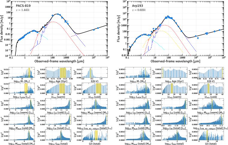
Figure 1. Two examples of our SED fitting for PACS-819 (left) and Arp 193 (right) with our MiChi2 code as described in Section 3. Upper panels show the best-fit SED (black line) and SED components, which are stellar (cyan dashed line), mid-IR AGN (yellow dashed line, optional if AGN is present), PDR dust (red dashed line), and cold/ambient dust (blue dashed line). Photometry data are shown by circles with error bars or downward-pointing arrows for upper limits if S/N < 3. Lower panels show 1/χ2 distributions for several galaxy properties from our SED fitting. In each subpanel, the height of the histogram indicates the highest 1/χ2 in each bin of the x-axis galaxy property. A higher 1/χ2 means a better fit. The 68% confidence level for our five SED component fitting is indicated by the yellow shading. (Figures for all sources are available at 10.5281/zenodo.3958271).
Download figure:
Standard image High-resolution imageOur code can also handle an arbitrary number of SED libraries as the components of the whole SED. For example, we use five SED libraries/components representing stellar, AGN, DL07 warm dust, DL07 cold dust, and radio emissions (see below). Our code samples their combinations in the five-dimensional space, then generates a composite SED (after multiplying the model with the filter curves), and then fits to the observed photometric data and obtains χ2 statistics. The post-processing of the χ2 distribution provides the best-fit and probability range of each physical parameter in the SED libraries (following Press et al. 1992, chapter 15.6).
Details of the five SED libraries/components are as follows:
- 1.Stellar component: for high-redshift (z > 1) SFGs, we use the Bruzual & Charlot (2003) code to generate solar metallicity, constant star formation history (SFH), and Chabrier (2003) IMF SED templates and then apply the Calzetti et al. (2000) attenuation law with a range of E(B − V) = 0.0−1.0 to construct our SED library. For local galaxies, we use the FSPS (Conroy et al. 2009; Conroy & Gunn 2010a, 2010b) code to generate solar -metallicity, τ-declining SFH, Chabrier (2003) IMF SED templates (also with the Calzetti et al. 2000 attenuation law), as this generates a larger variety of SED templates that fit local galaxies better.
- 2.
- 3.DL07 warm dust component for dust grains exposed to the PDR ISRF with intensity ranging from
 to in a power-law PDF with an index of −2 (updated version; see Draine et al. 2014; Aniano et al. 2020). The fraction of dust mass in polycyclic aromatic hydrocarbons (PAHs) is described by qPAH. The contribution of such warm dust to total ISM dust in mass is described by fPDR in this work (i.e., the γ in DL07). Free parameters are , qPAH, and fPDR.
 - 4.DL07 cold-dust component for dust grains exposed to the ambient ISRF with intensity of. The and qPAH of the cold dust are fixed to be the same as the warm dust in our fitting.
- 5.Radio component: a simple power-law with index −0.8 is assumed. Our code has the option to fix the normalization of the radio component at rest-frame 1.4 GHz to the total IR luminosity LIR(8–1000 μm) (integrating warm- and cold-dust components only) via assumptions about the IR−radio correlation (e.g., Condon et al. 1991; Yun et al. 2001; Ivison et al. 2010; Magnelli et al. 2015) when galaxies lack sufficient IR photometric data and display no obvious radio excess due to AGNs (e.g., Liu et al. 2018). As radio is not the focus of this work, we only use the simple power-law assumption for illustration purposes.


Note that we do not balance the dust-attenuated stellar light with the total dust emission. This has the advantage of allowing for optically thick dust emission that is only seen in the infrared. Our fitting then outputs χ2 distributions for the following parameters of interest (see bottom panels in Figure 1):
- 1.Stellar properties, including stellar mass M⋆, dust attenuation E(B − V), and light-weighted stellar age.
- 2.AGN luminosity LAGN, integrated over the AGN SED component.
- 3.IR luminosities for cold dust (LIR,cold dust), warm dust (LIR,PDR dust) and their sum (LIR,total dust).
- 4.Mean ISRF intensity, minimum ISRF intensity , and the mass fraction of warm/PDR-like dust in the DL07 model fPDR.


In Figure 1 we show two examples of our SED fitting. Best-fit parameters and their errors are also listed in our full sample table (Table 1 online version).
To verify our SED fitting, we also fit our high-z galaxies' SEDs with MAGPHYS and CIGALE (see more details in Appendix C). We find that for most high-z galaxies the stellar masses and IR luminosities agree within ∼0.2–0.3 dex. The IR luminosities are more consistent than stellar masses among the results of three fitting codes, with a scatter of ∼0.2 dex. In several outlier cases, our code produces more reasonable fitting to the data (e.g., AzTEC-3, Arp220, NGC 0253), which is likely because we do not have an energy balance constraint in the code. Our code has no systematic bias against CIGALE, but there is a noticeable trend that MAGPHYS fits slightly larger stellar masses than the other two. A possible reason is the use of the Charlot & Fall (2000) double attenuation law in MAGPHYS (see Lo Faro et al. 2017) rather than the Calzetti et al. (2000) attenuation law in our MiChi2 and CIGALE fitting.
Given the general agreement between our code and CIGALE/MAGPHYS, and to be consistent within this paper, we fit all SEDs with our MiChi2 SED fitting code with the five SED libraries as mentioned above.
4. ISRF Traces CO Excitation: The –R52 Correlation

We use our SED fitting results and the compiled CO data to study the empirical correlation between the CO (5–4)/CO (2–1) line ratio R52 and the mean ISRF intensity  . This correlation physically links molecular gas and dust properties together, supporting the idea that gas and dust are generally mixed together at large scales and exposed to the same local ISRF.
In Figure 2 we correlate R52 with various galaxy properties derived from our SED fitting. Panel (a) shows a tight correlation between R52 and the ambient ISRF intensity  , and panel (b) confirms the tight correlation between R52 and
  that was first reported by Daddi et al. (2015). Panels (c) and (d) show that CO excitation is also well correlated with galaxies' dust luminosities, but not with their stellar masses. In panels (e)−(g), we show that R52 exhibits no correlation with fPDR and mid-IR AGN fraction, while a very weak correlation seems to exist between R52 and the offset to the MS SFR, SFR/SFRMS. In each panel, the Pearson correlation coefficient P is computed and shown in the lower right corner. These correlations, or lack thereof, demonstrate that R52 or mid-J CO excitation is indeed mostly driven by dust-related quantities, i.e., LIR,
  , and
, and  .
.
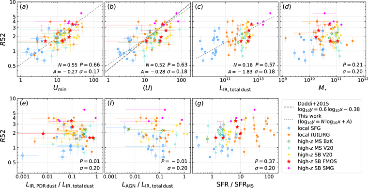
Figure 2. CO (5–4) to(2–1) line ratio R52 vs. various galaxy properties: (a) ambient ISRF intensity ( ); (b) mean ISRF intensity (
 ); (c) dust IR luminosity; (d) stellar mass; (e) luminosity fraction of dust exposed to warm/PDR-like ISRF to total dust in ISM (does not include AGN torus); (f) luminosity ratio between mid-IR AGN and total ISM dust (AGN luminosity is integrated over for all available wavelengths, while dust luminosity is integrated over rest-frame 8–1000 μm); and (g) the offset to the MS in terms of SFR. The Pearson coefficient P and scatter σ for each correlation are shown in the lower right corner. We performed orthogonal distance regression (ODR) linear regression fitting to the data points and their x and y errors in panels (a)–(c), where P > 0.5. Dotted lines are the best fits from this work, with slope N and intercept A shown at the bottom. The dashed line in panel (b) is the best-fit linear regression from Daddi et al. (2015).
Download figure:
Standard image High-resolution imageOur best-fitting R52– correlation is close to the one found by Daddi et al. (2015), yet somewhat shallower than that. Valentino et al. (2020a) also reported a shallower slope of the R52–
 correlation, given that the high-z V20 sample is used in both their and this work. Indeed, subsamples behave slightly differently in Figure 2. While local SFGs and local (U)LIRGs are scattered well around the average R52–
 correlation line, high-z MS and SB galaxies from the FMOS and V20 subsamples tend to lie below it. Given the varied S/N of IR data as reflected by the
  error bars, the majority of those high-z galaxies do not have a high-quality constraint on
  . High-z sample selections for CO observations are usually also biased to high-z IR-bright galaxies. Therefore, it is difficult to draw a conclusion about any redshift evolution of the R52–
 correlation with the current data set.
From panel (f) of Figure 2, we can see that there are several galaxies showing a high AGN-to-ISM dust luminosity ratio (note that the AGN luminosity is integrated over all wavelengths, while the IR luminosity is only DL07 warm+cold dust integrated over 8–1000 μm). The three galaxies with LAGN,allλ /LIR,8–1000μm ≳ 0.9 are V20-ID38986, V20-ID51936, and V20-ID19021, from high to low, respectively. They all clearly show power-law shape SEDs from the near-IR IRAC bands to mid-IR MIPS 24 μm and PACS 100 μm. 27 However, their R52 do not tend to be higher. This likely supports that these mid-J (Ju ∼ 5) CO lines are not overwhelmingly affected by AGNs.
We note that the correlations in Figure 2 are not the only ones worth exploring. R52 also correlates with dust mass in a way similar to  but with larger scatter, and
  can be considered as the ratio of LIR/Mdust; therefore, here we omit the correlation with Mdust. Daddi et al. (2015) also investigated how SFR surface density (ΣSFR), star formation efficiency (SFR/Mgas), gas-to-dust ratio (δGDR), and massive star-forming clumps affect
  and R52. Their results support the idea that a larger fraction of massive star-forming clumps with denser molecular gas compared to the diffuse, low-density molecular gas is the key for a high CO excitation (as proposed by the simulation work of Bournaud et al. 2015). Therefore, to understand the key physical drivers of CO excitation, information on molecular gas density distributions is likely the most urgently required.
5. Modeling of Molecular Gas Density Distribution in Galaxies
CO line emission in galaxies arises mainly from the cold molecular gas, and CO line ratios/SLEDs are sensitive to local molecular gas physical conditions, i.e., volume density  , column density
  , and kinetic temperature Tkin. These properties typically vary by one to three orders of magnitude within a galaxy, e.g., as seen in observations as reviewed by Young & Scoville (1991), Solomon & Vanden Bout (2005), Carilli & Walter (2013), and Combes (2018) and references therein, and also in modeling and simulations, e.g., by Krumholz & Thompson (2007), Glover & Clark (2012), Smith et al. (2014b), Narayanan & Krumholz (2014), Bournaud et al. (2015), Glover et al. (2015), Glover & Smith (2016), Popping et al. (2016, 2019), Renaud et al. (2019b, 2019a), and Tress et al. (2020).
In practice, studies of the CO SLED at a global galaxy scale or at subkiloparsec scales usually require the presence of a relatively dense gas component ( Tkin ≳ 50–100 K) in addition to a relatively diffuse gas (
 Tkin ∼ 20–100 K), via non-local thermodynamic equilibrium (non-LTE) LVG radiative transfer modeling (e.g., Israel et al. 1995; Mao et al. 2000; Israel & Baas 2001, 2002, 2003; Weiß et al. 2001, 2005; Bradford et al. 2003; Zhu et al. 2003; Bayet et al. 2004, 2006, 2009; Papadopoulos et al. 2007, 2008, 2010a, 2010b, 2012; Hailey-Dunsheath et al. 2008, 2012; Panuzzo et al. 2010; Rangwala et al. 2011; Papadopoulos et al. 2012; Spinoglio et al. 2012; Meijerink et al. 2013; Pereira-Santaella et al. 2013; Rigopoulou et al. 2013; Greve et al. 2014; Kamenetzky et al. 2014, 2016, 2017; Lu et al. 2014, 2017; Rosenberg et al. 2014a, 2014b; Schirm et al. 2014, 2017; Zhang et al. 2014; Israel et al. 2015; Liu et al. 2015; Mashian et al. 2015; Wu et al. 2015; Yang et al. 2017; Valentino et al. 2020a). A third state that is mostly responsible for Ju ≳ 10 CO lines is also found in the case of AGNs (e.g., van der Werf et al. 2010; Rangwala et al. 2011; Spinoglio et al. 2012) or mechanical heating (e.g., Rosenberg et al. 2014a). Therefore, a mid-J-to-low-J CO line ratio like R52 reflects not only the excitation condition of a single gas state but also the relative amount of the denser and warmer to the more diffuse gas component.
Leroy et al. (2017) have conducted pioneer modeling of the sub-beam gas density PDF to understand line ratios of CO isotopologue and dense gas tracers. The method includes constructing a series of one-zone clouds, performing non-LTE LVG calculation, and compositing line fluxes by the gas density PDF. They demonstrated that such modeling can successfully reproduce observed isotopologue or dense gas tracers to CO line ratios. Inspired by this work, we present in this section similar sub-beam density–PDF gas modeling to study the CO excitation and propose a useful conversion from R52 observations to  and Tkin for galaxies at global scales.
5.1. Observational Evidences of Gas Density PDF
Observation of gas density PDF at molecular cloud scale requires high angular resolution (e.g., sub-hundred-parsec scales) and full spatial information; therefore, it could only be obtained either with sensitive single-dish mapping in the Galaxy and nearest large galaxies or with sensitive interferometric plus total power observations. For external galaxies, the MAGMA survey by Pineda et al. (2009), Hughes et al. (2010), and Wong et al. (2011) mapped CO (1–0) in the LMC at 11 pc resolution with the Mopra 22 m single-dish telescope. Gardan et al. (2007), Gratier et al. (2010), and Druard et al. (2014) mapped M33 CO (2–1) emission at 50 pc scale with the IRAM 30 m single-dish telescope. The PAWS survey provides M51 CO maps at 40 pc obtained with the IRAM PdBI and with IRAM 30 m data (Hughes et al. 2013; Pety et al. 2013; Schinnerer et al. 2013; Leroy et al. 2016; Schinnerer et al. 2017). The ongoing PHANGS-ALMA survey 28 maps CO (2–1) at ∼60–100 pc scales in more than 70 nearby galaxies using ALMA with total power (A. Leroy et al. 2021, in preparation; see also Kreckel et al. 2018; Sun et al. 2018, 2020; Schinnerer et al. 2019; Chevance et al. 2020). Meanwhile, higher physical resolution observations are also available for Galactic clouds and filaments, e.g., Kainulainen & Tan (2013), Lombardi et al. (2014, 2015), Kainulainen & Federrath (2017), and Zhang et al. (2019), to name a few.
These observations at large scales reveal a smooth gas density PDF that can be described by a lognormal distribution plus a high-density power-law tail (e.g., Wong et al. 2011; Hughes et al. 2013; Druard et al. 2014). The width of the lognormal PDF and the slope of the power-law tail do slightly vary among galaxies, but the most prominent difference is seen for the mean of the lognormal PDF (hereafter  ), which changes by more than one order of magnitude (for a relatively small sample of <10 spiral galaxies; see Figure 7 of Leroy et al. 2016).
Interestingly, such a lognormal PDF is consistently predicted by isothermal homogeneous supersonic turbulent theories or diverse cloud models (e.g., Ostriker et al. 2001; Vázquez-Semadeni & García 2001; Padoan & Nordlund 2002; Padoan et al. 2004a, 2004b; Tassis et al. 2010; Padoan & Nordlund 2011; Padoan et al. 2012; Kritsuk et al. 2017; Raskutti et al. 2017; see also references in Raskutti et al. 2017), and the additional power-law PDF is also expected, e.g., for a multiphase ISM and/or due to the cloud evolution/star formation at late times (e.g., Klessen et al. 2000; Tassis et al. 2010; Kritsuk et al. 2017; Raskutti et al. 2017 and references therein). Therefore, modeling gas density PDFs assuming a lognormal distribution plus a power-law tail appears to be a very reasonable approach.
5.2. Sub-beam Gas Density PDF Modeling
We thus assume that the line-of-sight volume density of molecular gas in a galaxy follows a lognormal PDF, with a small portion of lines of sight following a power-law PDF at the high-density tail. Representative PDFs are shown in Figure 3. Each PDF samples the  from 1 to 107 cm−3 in 100 bins in logarithmic space. For each
  bin, the height of the PDF is thus proportional to the number of sight lines with a density of
  . We assume that the CO line emission surface brightness from each line of sight can be computed from an equivalent "one-zone" cloud with a single
  ,
,  , Tkin, velocity gradient, and CO abundance. Thus, the total CO line emission surface brightness is the sum of all sight lines in the PDF.
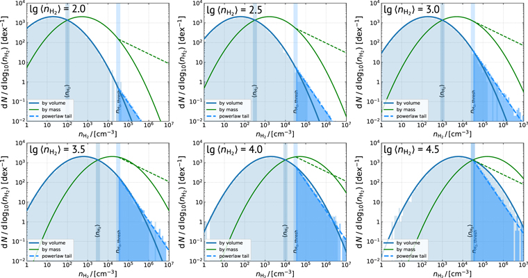
Figure 3. Example of composite gas density PDFs in our modeling with varied lognormal PDFs mean gas density  (from 2.0 to 4.5 in panels from left to right and top to bottom) and a fixed power-law tail threshold gas density
  . The
. The  and
and  are indicated by the vertical transparent bars and labels in each panel. The thick blue and thin green solid (dashed) lines represent the volume- and mass-weighted PDFs of the lognormal (power-law tail) gas component, respectively.
Download figure:
Standard image High-resolution imageThe shape of the gas density PDF is described by the following parameters: the mean gas density of the lognormal PDF  , the threshold density of the power-law tail
  , the width of the lognormal PDF, and the slope of the power-law tail. We model a series of PDFs by varying the
  from 102.0 to 105.0 cm−3 in steps of 0.25 dex and
  from 104.0 to 105.25 cm−3 in steps of 0.25 dex, to build our model grid, which can cover most situations observed in galaxies. The slope of the power-law tail is fixed to −1.5, which is an intermediate value as indicated by simulations (Federrath & Klessen 2013), also previously adopted by Leroy et al. (2017). The width of the lognormal PDF is physically characterized by the Mach number of the supersonic turbulent ISM (see Padoan & Nordlund 2002, 2011 and Equation (5) of Leroy et al. 2017):
  , which ranges typically from 4 to 20 in star-forming regions as shown by simulations (e.g., Krumholz & McKee 2005; Padoan & Nordlund 2011). Here we adopt a fiducial Mach number of 10, as done previously by Leroy et al. (2017). Note that a high Mach number of ∼80 is also found in merger systems and SB galaxies (e.g., Leroy et al. 2016). It corresponds to a lognormal PDF width 1.56× our fiducial value and marginally affects the CO excitation in a similar way to a higher
  . Thus, for simplicity in this work we fix the Mach number and allow
  to vary.
5.3. One-zone Gas Cloud Calculation
For a given gas density PDF, each  bin is composed of the same "one-zone" gas clouds for which we will compute the line surface brightness. A one-zone cloud has a single volume density
  , column density
  , gas kinetic temperature (Tkin), CO abundance [CO/H2], and velocity gradient dv/dr. Note that although an equivalent cloud size r is implied from the ratio of
  and
and  , given that the calculation is in 1D, r should not be taken as a physical cloud size. Also note that in our study we do not model the 3D distribution of one-zone models; therefore, any radiative coupling between one-zone models along the same line of sight cannot be accounted for. This is likely a minor issue for star-forming disk galaxies given their thin disks (a few hundred parsecs; Wilson et al. 2019) and systematic rotation that separates molecular clouds in the velocity space for inclined disks, but the actual effects need to be studied by detailed numerical simulations (e.g., Smith et al. 2020; Tress et al. 2020).
Here we use RADEX (van der Tak et al. 2007) to compute the 1D non-LTE radiative transfer. For a given  , we loop
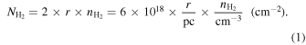
  from 1021 to 1024 cm−2, and r is then determined by
We also loop over Tkin values of 25, 50, and 100 K, while we fix [CO/H2] = 5 × 10⁻⁵, a reasonable guess for star-forming clouds (e.g., Leung & Liszt 1976; van Dishoeck & Black 1987, 1988), although it varies from cloud to cloud and depends on chemistry (e.g., Sheffer et al. 2008). Note that there is one additional free parameter to set, i.e., the LVG velocity gradient dv/dr, or the line width FWHM ΔV, or the velocity dispersion σV . They are related to each other by
To determine these quantities and effectively reduce the number of free parameters while being consistent with observations, we use an empirical correlation between  , r, σV
, and the virial parameter αvir. αvir describes the ratio of a cloud's kinetic energy and gravitational potential energy (e.g., Bertoldi & McKee 1992) and can be written as
, r, σV
, and the virial parameter αvir. αvir describes the ratio of a cloud's kinetic energy and gravitational potential energy (e.g., Bertoldi & McKee 1992) and can be written as  , where σV
and r are introduced above, G is the gravitational constant, M is the cloud mass, and f is a factor to account for the lack of balance between kinetic and gravitational potential (see Equation (6) of Sun et al. 2018). Observations show that clouds are not always virialized, i.e., αvir is not always unity. Based on ∼60 pc CO mapping of 11 galaxies in the PHANGS-ALMA sample, Sun et al. (2018) reported the following correlation in their Equation (13) (helium and other heavy elements are included; see also Equation (2) in the review by Heyer & Dame 2015):
, where σV
and r are introduced above, G is the gravitational constant, M is the cloud mass, and f is a factor to account for the lack of balance between kinetic and gravitational potential (see Equation (6) of Sun et al. 2018). Observations show that clouds are not always virialized, i.e., αvir is not always unity. Based on ∼60 pc CO mapping of 11 galaxies in the PHANGS-ALMA sample, Sun et al. (2018) reported the following correlation in their Equation (13) (helium and other heavy elements are included; see also Equation (2) in the review by Heyer & Dame 2015):
They find αvir ≈ 1.5–3.0 with a 1σ width of 0.4–0.65 dex. For simplicity and also with the idea of focusing primarily on the effect of gas density, we adopt a constant αvir of 2.3. As shown in later sections, this is already sufficient to explain the observed CO line ratios/SLEDs by our modeling. But note that more comprehensive descriptions of αvir can be achieved in simulations and can be compared with the results from this work to better understand how a changing αvir could affect CO line ratio prediction.
Figure 4 presents how R52 changes with the gas densities of one-zone cloud models for four representative redshifts where the cosmic microwave background (CMB) temperatures are different. We repeat our calculations for three representative Tkin as labeled in each panel. The comparison shows that Tkin significantly affects the R52 line ratio, especially at low densities and at low redshifts. Note that due to the constant αvir assumption, for a given  , Equation (3) implies that σV
∝ r and that dv/dr is not varying with
, Equation (3) implies that σV
∝ r and that dv/dr is not varying with  . Thus, the actual choices of
  (or r) for each single one-zone model will not affect the modeling of R52 (and of the optical depth τ).

Figure 4. CO (5–4)/CO (2–1) line ratio (R52) from single one-zone LVG calculation. The four panels show the calculations at four representative redshifts z = 0, 1.5, 4, and 6, from left to right, respectively. Solid, dashed, and long-dashed lines are for gas kinetic temperature Tkin = 25, 50, and 100 K, respectively. The gray lines in the second, third, and fourth panels are the corresponding z = 0 lines.
Download figure:
Standard image High-resolution imageIn addition, our modeling is also able to produce reasonable line optical depths (τ) and [C i]/CO line ratios, as presented in Appendix D.
5.4. Converting R52 to and Tkin with the Model Grid

We compute the global line surface brightness by summing one-zone line surface brightnesses at each  bin according to the gas density PDF. With our assumptions, there are only four free parameters: the mean gas density of the lognormal PDF
  , the threshold density of the power-law tail
  , gas kinetic temperature Tkin, and redshift. Their grids are described in Section 5.2.
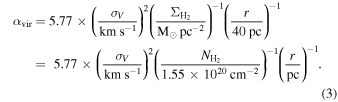
In Figure 5, we present the predicted R52 as a function of the four free parameters. R52 increases smoothly with  and Tkin, while
  does not substantially alter the R52 ratio, as indicated by the color-coding. The minimum R52 at the lowest density (
 ) is nearly doubled from redshift 0 to 6 owing to the increasing CMB temperature, but such a redshift effect is less prominent (<×1.5) both at higher density (
 ) and for higher Tkin.
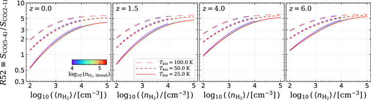
Figure 5.
R52 as functions of the mean gas density ( ) as predicted from our composite gas modeling. The four panels show the models at four different representative redshifts. In each panel, color indicates the threshold density of the power-law tail (
 which alters the line ratio only slightly), and three line styles are models at three representative kinetic temperatures (Tkin = 25, 50, and 100 K for solid, dashed, and long-dashed lines, respectively).
Download figure:
Standard image High-resolution imageIn Figure 6, we further show the full CO SLEDs at Ju = 1–9 from our model grid and compare them with a subsample of galaxies with multiple CO transitions at various redshifts. These galaxies are displayed in panels where the  is closest to their R52-derived
  (see below). Our modeling can generally match these CO SLEDs given certain choices of
  and Tkin. Yet we caution that this is not a thorough comparison, and our model grid might not fit entirely well the CO SLED shape owing to our simplifying assumptions of fixed Mach number and power-law tail slope or αvir. While this work only focuses on R52 with the simplest assumptions, the model predictions seem overall already quite promising for the whole CO SLEDs and can be further improved in future works.
Figure 6. Predicted CO SLEDs in Jansky units and normalized at CO (2–1). From top to bottom, CO SLEDs are at redshift z = 0, 1.5, 4, and 6, respectively. And from left to right, lognormal PDFs mean gas density  changes from 2.0 to 5.0 in steps of 0.5. In each panel, solid, dashed, and long-dashed lines represent Tkin = 25, 50, and 100 K models, respectively. Line color-coding indicates the threshold gas density of the power-law tail PDF,
  . Colored data points are CO line fluxes in the following galaxies, with references in parentheses: the Milky Way (Fixsen et al. 1999), local spiral M51 (Schirm et al. 2017), local ULIRGs Mrk 231, IRAS F18293–3413, and IRAS F17207–0014 (L15, Kamenetzky et al. 2014), z = 1.5 BzK galaxies (Daddi et al. 2015), z = 1.5 starburst galaxies (Silverman et al. 2015b and this work). z = 4.055 SMG GN20 (Daddi et al. 2009; Carilli et al. 2010; Tan et al. 2014), z = 4.755 SMG ALESS73.1 (Coppin et al. 2010; Zhao et al. 2020), z = 5.3 SMG AzTEC-3 (Riechers et al. 2010), and z = 6.3 SMG HFLS3 (Riechers et al. 2013).
Download figure:
Standard image High-resolution imageBased on the model grid, we describe below a method to determine the most probable  , Tkin, and
  ranges for a given R52 and its error in galaxies with known redshift. This is done with a Monte Carlo approach. We first interpolate our 4D model grid to the exact redshift of each galaxy using Python
scipy.interpolate.LinearNDInterpolator and then resample the 3D model grid to a finer grid, perturb the R52 given its error over a normal distribution for 300 realizations, and find the minimum χ2 best fits for each realization. Finally, we combine best fits to obtain posterior distributions of
ranges for a given R52 and its error in galaxies with known redshift. This is done with a Monte Carlo approach. We first interpolate our 4D model grid to the exact redshift of each galaxy using Python
scipy.interpolate.LinearNDInterpolator and then resample the 3D model grid to a finer grid, perturb the R52 given its error over a normal distribution for 300 realizations, and find the minimum χ2 best fits for each realization. Finally, we combine best fits to obtain posterior distributions of  , Tkin, and
  and determine their median, 16th percentile (L68), and 84th percentile (H68). This fitting method is coded in our Python package co-excitation-gas-modeling that is made publicly available.
We note that although there is a single input observation (R52) whereas there are three parameters to be determined ( , Tkin, and
  ), our method still produces reasonable results. In fact, our method is able to take into account the internal degeneracy between
  and Tkin inside model grids, thus obtaining reasonable probability ranges. Figure 7 shows the fitted
  and Tkin for our galaxy sample, resulting in a nonlinear trend between
  and Tkin. The galaxy-wide mean pressures of gas can also be calculated as
  and are found to agree with estimates in local galaxies (Kamenetzky et al. 2014).
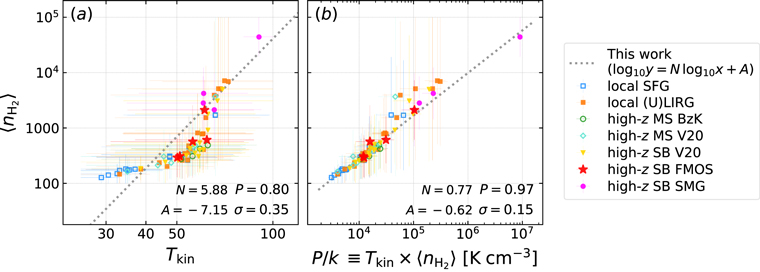
Figure 7. Fitted mean gas density  vs. fitted gas kinetic temperature Tkin (left panel) and gas pressure P/k (right panel; k is the Boltzmann constant) based on R52 and its errors in our galaxy sample. This reflects the internal degeneracy between
  and Tkin in our model grid. See fitting method in Section 5.4.
Download figure:
Standard image High-resolution imageIn Figures 8 and 9, we present correlations between the R52-fitted  and Tkin, respectively, and various galaxy properties, similarly to what is presented in Figure 2 for R52. We discuss them in detail in the next sections (Section 6.2).
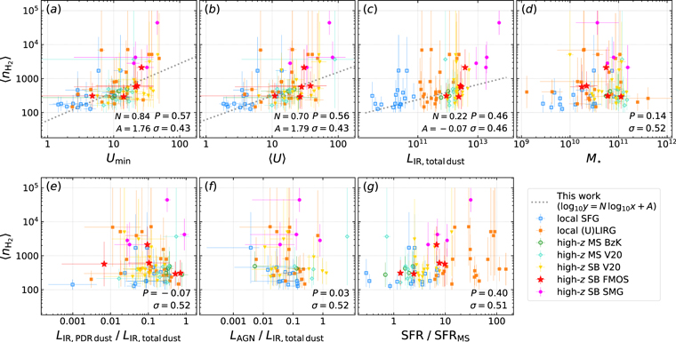
Figure 8. Fitted  vs. galaxy properties, as in Figure 2. Data points'
  and error bars are the median and 1σ ranges of the fitting using our model grid as presented in Section 5 to the observed R52.
Download figure:
Standard image High-resolution image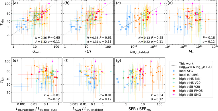
Figure 9. Fitted Tkin vs. galaxy properties, as in Figure 2. Tkin is shown as median and error bars representing the 1σ range of our model grid fitting to the observed R52 as presented in Section 5.
Download figure:
Standard image High-resolution image6. Results on ISM Physical Properties and Discussion
6.1. The Underlying Meaning of : A Mass-to-light Ratio for Dust

By definition,  is the mass-weighted ISRF intensity created by UV photons from stars in a galaxy. As indicated by the DL07 model and many of its applications, e.g., Draine et al. (2007, 2014), Aniano et al. (2012, 2020), Dale et al. (2012, 2017), Magdis et al. (2012, 2017), Ciesla et al. (2014) and Schreiber et al. (2018),
  is actually a mass-weighted, average mass-to-light ratio for the mixture of dust grains in a galaxy. It is driven by the young stars emitting most of the UV photons, but it also reflects the mean distance between young stars and interstellar dust and the efficiency of UV photons heating the dust. For a given DL07 ISRF distribution power-law index (=−2) and
  (=107; Draine et al. 2014),
  is proportional to the ratio between LIR and Mdust, with a coefficient P0 ≈ 138 from this work, where P0 represents the power absorbed per unit dust mass in a radiation field U = 1:
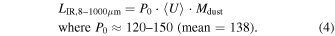
Note that the P0 factor is calibrated to be equal to 125 in Magdis et al. (2012) owing to a slightly different  , a small 10% systematic difference.
 is also positively linked to dust temperature, but it depends on how dust temperature is defined. For example, Draine et al. (2007) find that T ≈ 17 · U1/6 (K) for dust grains with sizes greater than 0.03 μm whose blackbody radiation peaks around 160 μm. Schreiber et al. (2018) calibrate the light-weighted dust temperature
  (and mass-weighted
  ) by fitting Wien's law to each elementary Galliano et al. (2011) template.
Studies of Tdust and  have shown that dust (ISRF) is warmer (stronger) for increasing IR luminosity from local SFGs to (U)LIRGs (e.g., Hwang et al. 2010; Symeonidis et al. 2013; Herrero-Illana et al. 2019) and increases with redshift for the majority of MS galaxies (e.g., Magdis et al. 2012; Magnelli et al. 2014; Béthermin et al. 2015; Schreiber et al. 2018). Some observations show colder dust temperatures in a few among the most extreme SB systems (e.g., Lisenfeld et al. 2000; Jin et al. 2019; Cortzen et al. 2020). These are likely due to the presence of high dust opacity at shorter wavelengths, which makes the dust SED apparently colder. Observations of SMGs also show colder dust temperatures in some of the less luminous ones. This phenomenon is likely driven by the fact that (sub)millimeter selection favors cold-dust galaxies whose SEDs peak closer to (sub)millimeter wavelengths (e.g., Chapman et al. 2005; Kovács et al. 2006; Symeonidis et al. 2009, 2011; Hwang et al. 2010; Magdis et al. 2010; Magnelli et al. 2010).
There is also an interesting finding that for extreme SB galaxies with SFR/SFRMS > 4 their  seem to not evolve with redshift (e.g., Béthermin et al. 2015), while
  in MS galaxies does evolve with redshift, and extrapolation. This suggests that
  in MS galaxies might become stronger than those in extreme SB galaxies at z > 2.5, which seems at odds with the expectation. Yet this finding might also be limited by sample size and selection method, templates used for SED fitting, and the dust optically thin assumption in DL07 templates (e.g., Jin et al. 2019; Cortzen et al. 2020).
Combining with the results from this work, the Tdust or  trends are easier to understand when correlating them with molecular gas mean density and temperature. We propose a picture in which the general increase of dust temperature and ISRF is mainly due to the increase in cold molecular gas temperature, due to either higher CMB temperature at higher redshifts or more intense star formation and feedback. While the mean molecular gas density has a weaker, nonlinear trend driving
  in most galaxies, merger-driven compaction could strongly increase gas density and hence boost
  , Tkin, and
  in a small number of SB galaxies. Such an increase in gas density creates more contrast at lower redshifts owing to the general decrease of the cosmic molecular gas density and CMB temperature. This could explain why
  is more different between MS and SB galaxies at lower redshifts.
6.2. Density- or Temperature-regulated Star Formation? The – and –Tkin Correlations


Figures 8 and 9 show that both  and Tkin positively correlate with U and LIR but not with other properties like stellar mass or AGN fraction in our sample. Yet
  correlates with U or LIR in a nonlinear way. Except for high-z SMGs and a few local galaxies with large error bars coming from their large R52 uncertainties, most galaxies are constrained within a narrow range of
  . Despite the large scatter in the data, we observe a trend with
  that seems to hold only within the intermediate
  range (
 ).
).
Meanwhile, Tkin has a tighter correlation (σ ∼ 0.11) with U and LIR. We find relations  and
and  . Note that by calculating the [Ci] 3
P2–3
P1 and 3
P1–3
P0 excitation temperatures as a probe of gas kinetic temperature under thermalized conditions, Jiao et al. (2017, 2019) and Valentino et al. (2020b) also found positive correlation between the gas kinetic temperature and dust temperature that is proportional to
. Note that by calculating the [Ci] 3
P2–3
P1 and 3
P1–3
P0 excitation temperatures as a probe of gas kinetic temperature under thermalized conditions, Jiao et al. (2017, 2019) and Valentino et al. (2020b) also found positive correlation between the gas kinetic temperature and dust temperature that is proportional to  . There is also a weak trend that Tkin increases with SFR/SFRMS (Pearson correlation coefficient P = 0.34), and the trend between
  and SFR/SFRMS is also marginal (P = 0.40).
Given these results, it is very reasonable that both mean gas density and temperature increase from less to more intensively SFGs. Yet based on the data sets in this work, it is difficult to statistically decouple  and Tkin and hence to measure well the shapes of
  –
– and
and  –Tkin correlations. However, the nonlinear or broken
  –
– correlation and the more smooth
  –Tkin might imply two scenarios, one for "normal" SFGs and one for merger-driven SBs. "Normal" galaxies may have a smooth density- and temperature-regulated star formation, whereas strong gas compression in major merger events can induce extraordinarily high
  with moderate Tkin and
  (e.g., Tacconi et al. 2008; Engel et al. 2010; Riechers et al. 2010; Cooray et al. 2014; Larson et al. 2016; Calabrò et al. 2019). Further insights will require higher-quality, multiple-transition CO SLEDs, as we briefly discuss below (Section 6.4).
6.3. Implication for Star Formation Law Slopes
The star formation law is known as the correlation between gas mass (or surface density) and SFR (or surface density) and can be expressed as
where A is the normalization and N is the slope. After the initial idea presented by Schmidt (1959), Kennicutt (1998) first systematically measured the star formation law to be  based on observations of nearby spiral and SB galaxies, where Σgas is the mass surface density of atomic plus molecular gas, and ΣSFR is the SFR surface density traced by Hα and/or LIR. This Kennicutt–Schmidt law with N ≈ 1.4 has been extensively studied in galaxies with Σgas ∼ 1–105
M⊙ pc−2 and is widely used in numerical simulations (see reviews by Kennicutt & Evans 2012; Carilli & Walter 2013).
based on observations of nearby spiral and SB galaxies, where Σgas is the mass surface density of atomic plus molecular gas, and ΣSFR is the SFR surface density traced by Hα and/or LIR. This Kennicutt–Schmidt law with N ≈ 1.4 has been extensively studied in galaxies with Σgas ∼ 1–105
M⊙ pc−2 and is widely used in numerical simulations (see reviews by Kennicutt & Evans 2012; Carilli & Walter 2013).
However, the actual slope N of the star formation law has been long debated. High-resolution (subkiloparsec-scale) observations in nearby spiral galaxies revealed that atomic gas does not correlate with SFR, whereas only molecular gas traces SFR, and N is close to unity in these galaxies (e.g., Wong & Blitz 2002; Bigiel et al. 2008; Leroy et al. 2008, 2013; Schruba et al. 2011). Meanwhile, from local SFGs to (U)LIRGs, observations suggest that N is superlinear, ranging from ∼1 to ∼2 (e.g., Kennicutt 1998; Yao et al. 2003; Gao & Solomon 2004a; Shetty et al. 2013, 2014b, 2014a; de los Reyes & Kennicutt 2019; Wilson et al. 2019). Furthermore, Daddi et al. (2010b) and Genzel et al. (2010) found that high-redshift MS and SB galaxies follow two parallel sequences in the star formation law ( –SFR) diagram, each with substantial breadth, and both with N ∼ 1.1–1.2 but with a 0.6 dex mean offset in normalization. Thus, why local SFG regions show a linear star formation law, while high-z SB galaxies have a much higher
  , is still to be understood.
Here we decompose the star formation law into  and
and  to gain some insights. First, it is known that the dust-obscured SFR can be traced by the IR luminosity (e.g., Kennicutt 1998; Kennicutt & Evans 2012) as SFR = LIR/CIR, where
 ![${C}_{\mathrm{IR}}\sim {10}^{10}\,[{L}_{\odot }\,{({M}_{\odot }{\mathrm{yr}}^{-1})}^{-1}]$](https://content.cld.iop.org/journals/0004-637X/909/1/56/revision2/apjabd801ieqn403.gif) assuming a Chabrier (2003) IMF. Second, as mentioned in the previous section,
assuming a Chabrier (2003) IMF. Second, as mentioned in the previous section,  . Third, we use the gas-to-dust ratio δGDR ≡ Mgas/Mdust to link gas to dust mass. This ratio varies with metallicity (e.g., Israel 1997; Leroy et al. 2007, 2011; Bolatto et al. 2013; Sandstrom et al. 2013; Rémy-Ruyer et al. 2014, 2015), and also note that the definition of gas in δGDR is atomic plus molecular gas. We include an additional molecular hydrogen fraction
  to the gas-to-dust ratio, having finally
  . Fourth, we consider MS galaxies to be disks with radius r and height h and assume that
  is the global mean gas density; thus, the molecular gas mass can be expressed as the product of the volume and the mean molecular gas density:
  . And fifth, we ignore atomic gas and only consider the molecular gas star formation law.
Then, we rewrite the star formation law equation as
Taking the logarithm of both sides, and assuming that  ,
,  , and
, and  are functions of
  , we have
Therefore, the star formation law slope N depends on how  ,
,  (metallicity), and r2
h (galaxy size) change with
(metallicity), and r2
h (galaxy size) change with  , which can further be described by the differentials
  ,
,  , and
, and  , respectively. These differentials strongly depend on galaxy samples. When studying subkiloparsec regions in local SFGs, if the ISRF, metallicity, and galaxy size are similar among these SFGs, N is close to 1. When studying a sample including both SFGs and (U)LIRGs,
  increases by a factor of a few tens with
  changing from 102 to 104 cm−3, and r decreases by a factor of a few with
  , as (U)LIRGs are usually smaller and more compact (while the scale height h seems constant; e.g., Wilson et al. 2019). As for the
  term, because
  increases with metallicity while δGDR decreases with it, their product
  likely does not change much. Therefore, N can be much higher than 1. The overall effect is that the star formation law does not have a single slope, yet the overall N is about 1–2.
6.4. Limitations and Outlook
We discuss three limitations of this work: the overall quality of current data sets, the assumptions in the gas modeling, and the contamination from AGNs. First, CO line ratio or SLED studies require two or more CO line observations. These observations have different observing conditions, beam sizes, flux calibrations, etc.; thus, uncertainties are very likely underestimated even when the S/Ns of the line measurements are formally large (e.g., >3). For example, for our local SFG subsample, CO (5–4) data are from the Herschel FTS with a certain beam size of ∼40'', which does not match the mapping area of CO (2–1) from ground-based telescopes. The correction from the FTS beam to the entire galaxy can have a factor of two difference, which is reflected in the scatter of our data points although not fully reflected in their error bars. The absolute flux calibration uncertainty of the observations in the literature can also be as high as ∼30%, which is much poorer than current IRAM 30 m and ALMA (total power) observations (<10%). This also increases the scatter in our plots and necessarily makes observed correlations less significant. As for high-redshift galaxies, we use an S/N of 3 in both CO lines to select our sample, which usually only reflects the quality of line measurements, while it does not include the absolute flux calibration uncertainty. Their dust SEDs are also much more poorly covered; thus, their  have fairly large uncertainties. Future ALMA Band 3–8 mapping of CO lines from Ju = 1 to 4 in local galaxies and VLA plus ALMA observations for suitable galaxies at high redshift with high-quality CO and continuum data will be the key to both spatially understand and statistically verify correlations between
  ,
,  , and Tkin, as well as to unveil any evolutionary trend with redshift.
Second, our assumptions in the gas modeling are also simplistic, in order to reflect only the effects of density and temperature on CO excitation. The constant αvir assumption does not reflect the real situation in galaxies, e.g., as shown in Sun et al. (2018). Doubling the αvir value from what we use in this work will result in a 20% lower R52 at  , Tkin = 25 K, and z = 0. The constant Tkin assumption for all one-zone clouds in a galaxy is also a simplified "toy model"-like condition. Adopting more realistic assumptions from observations (e.g., Sun et al. 2020) or from hydrodynamic+chemistry simulations (e.g., Smith et al. 2014a, 2014b, 2016, 2020; Tress et al. 2020) in our gas modeling would naturally be the next step.
Third, it is known that some galaxies host AGNs that significantly contribute to optical or mid-IR SEDs, as well as affect the CO excitation. Our SED fitting has already included a mid-IR AGN component that can dominate rest-frame 5–50 μm emission. This substantially improves the fitting χ2 for a number of galaxies showing mid-IR power-law SED features, which, however, also brings in larger uncertainties in  as reflected in the error bars in our plots. The used AGN SED templates could also slightly affect our results, although this effect should be well captured by the quoted uncertainties. Additional mid-IR photometry from future space telescopes like the James Webb Space Telescope (JWST) and the Origins Space Telescope (OST) will be key to solve this degeneracy and provide accurate AGN/ISRF decomposition. Meanwhile, an AGN can also boost highly excited CO lines within X-ray-dominated regions (XDRs) as shown by Ju ≳ 9 CO studies (e.g., van der Werf et al. 2010; Rangwala et al. 2011; Hailey-Dunsheath et al. 2012; Spinoglio et al. 2012; Meijerink et al. 2013; Pereira-Santaella et al. 2013; Rosenberg et al. 2014a). Decomposition of such AGN-dominated CO SLEDs usually requires three components, but the XDR component starts to dominate the CO SLED only at Ju ≳ 9. Thus, for this work, at CO (5–4) AGNs likely contribute less than 10% (e.g., see Figure 2 of van der Werf et al. 2010).
7. Summary
In this work, we compiled a comprehensive sample of galaxies from local to high redshift with CO (2–1) and CO (5–4) detections and well-sampled IR SEDs. This includes our new IRAM PdBI CO (5–4) observations of six z ∼ 1.5 COSMOS SB galaxies. With this large sample, we measure their mean ISRF intensity  from dust SED fitting (Section 3) and their mean molecular gas density
  converted from R52 = SCO(5-4)/SCO(2-1) line ratios based on our density–PDF gas modeling (Section 5). Our results can be summarized as follows.
- 1.
- 2.We conduct density–PDF gas modeling to connect the mean molecular gas density and kinetic temperature Tkin to the observable CO line ratio R52. Based on this, we provide a Monte Carlo method (and a Python package co-excitation-gas-modeling) to compute and Tkin's probability ranges using our model grid for any given Ju = 1–10 CO line ratio (and for CO SLED as the next step; see, e.g., Figure 6).
- 3.We find that both and Tkin increase with , with Tkin having a tighter correlation with .
- 4.Based on these correlations, we propose a scenario in which the ISRF in the majority of galaxies is more directly regulated by the gas temperature and nonlinearly by the gas density. A fraction of SB galaxies have gas densities larger by more than one order of magnitude with respect to MS galaxies and are possibly in a merger-driven compaction stage (Sections 6.2 and 6.1).
- 5.We link the– correlation to the Kennicutt–Schmidt star formation law and discuss how the star formation law slope N can be inferred from the – correlation slope and other galaxy properties versus correlations. We find that N ∼ 1–2 can be inferred from the trends of how and galaxy size change with in different galaxy samples (Section 6.3).


Our study demonstrates that ISRF and molecular gas are tightly linked to each other, and density–PDF gas modeling is a promising tool for probing detailed ISM physical quantities, i.e., molecular gas density and temperature, from observables like CO line ratios/SLEDs.
We thank the anonymous referee for helpful comments. D.L., E.S., and T.S. acknowledge funding from the European Research Council (ERC) under the European Union's Horizon 2020 research and innovation program (grant agreement No. 694343). F.V. acknowledges support from the Carlsberg Foundation Research Grant CF18-0388 "Galaxies: Rise and Death". G.E.M. and F.V. acknowledge the Villum Fonden research grant 13160 "Gas to stars, stars to dust: tracing star formation across cosmic time" and the Cosmic Dawn Center of Excellence funded by the Danish National Research Foundation under then grant No. 140. Y.G.'s research is supported by the National Key Basic Research and Development Program of China (grant No. 2017YFA0402700), National Natural Science Foundation of China (grant Nos. 11861131007, 11420101002), and Chinese Academy of Sciences Key Research Program of Frontier Sciences (grant No. QYZDJSSW-SLH008). S.J. acknowledges financial support from the Spanish Ministry of Science, Innovation and Universities (MICIU) under grant AYA2017-84061-P, co-financed by FEDER (European Regional Development Funds). A.P. gratefully acknowledges financial support from STFC through grants ST/T000244/1 and ST/P000541/1. We thank A. Weiss and C. Wilson for helpful discussions. This work used observations carried out under project No. W14DS with the IRAM Plateau de Bure Interferometer (PdBI). IRAM is supported by INSU/CNRS (France), MPG (Germany), and IGN (Spain). This work used observations carried out under project 17A-233 with the National Radio Astronomy Observatory's Karl G. Jansky Very Large Array (VLA). The National Radio Astronomy Observatory is a facility of the National Science Foundation operated under cooperative agreement by Associated Universities, Inc.
Data Availability
Our MiChi2 SED fitting code is publicly available at https://ascl.net/code/v/2533. Our Python package co-excitation-gas-modeling for computing  and Tkin from CO line ratios is publicly available at https://pypi.org/project/co-excitation-gas-modeling. And our SED fitting figures as shown in Figure 1 and the full Table 1 are publicly available at 10.5281/zenodo.3958271.
Appendix A: IRAM PdBI CO Observations of z ∼ 1.5 FMOS-COSMOS Galaxies
We present the sample table and CO (5–4) imaging of our PdBI observations in Table 2 and Figure 10. The observations are described in Section 2.2.
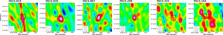
Figure 10. CO (5–4) line maps for PACS-819, PACS-830, PACS-867, PACS-299, PACS-325, and PACS-164, respectively. In the last two panels, PACS-325 and PACS-164 are undetected. The field of view is 12'' × 12'' in all panels. Contours have a spacing of 1σ noise in each panel. The cross-hair indicates the phase center, and the box indicates the ALMA CO (2–1) emission peak position, which is also the position where we extract the CO (5–4) line fluxes.
Download figure:
Standard image High-resolution imageTable 2. CO Observation Results
| Source | R.A.CO | Decl.CO | zCO | ΔVCO | CO Size | SCO(1−0) | SCO(2−1) | SCO(5−4) |
|---|---|---|---|---|---|---|---|---|
| (km s−1) | ('') | (Jy km s−1) | (Jy km s−1) | (Jy km s−1) | ||||
| (1) | (2) | (3) | (4) | (5) | (6) | (7) | (8) | (9) |
| PACS-819 | 09:59:55.552 | 02:15:11.70 | 1.4451 | 592 | 0.335 | ⋯ | 1.10 ± 0.07 | 3.850 ± 0.922 |
| PACS-830 | 10:00:08.746 | 02:19:01.87 | 1.4631 | 436 | 0.973 | ⋯ | 1.18 ± 0.10 | 1.876 ± 0.387 |
| PACS-867 | 09:59:38.078 | 02:28:56.73 | 1.5656 | 472 | ⋯ | 0.119 ± 0.064 | 0.46 ± 0.04 | 0.731 ± 0.218 |
| PACS-299 | 09:59:41.295 | 02:14:43.03 | 1.6483 | 590 | ⋯ | <0.210 a | 0.67 ± 0.08 | 1.758 ± 0.325 |
| PACS-325 | 10:00:05.475 | 02:19:42.61 | 1.6538 | 764 | ⋯ | ⋯ | 0.28 ± 0.06 | <0.942 a |
| PACS-164 | 10:01:30.530 | 01:54:12.96 | 1.6481 | 894 | ⋯ | <0.222 a | 0.61 ± 0.11 | 1.175 ± 0.465 |
Notes. Columns (1–6) and (8) are the ALMA CO (2–1) properties reported by Silverman et al. (2015b). Columns (7) and (9) show the results from this work for VLA CO (1–0) and IRAM PdBI CO (5–4), respectively.
a 3σ upper limits.Download table as: ASCIITypeset image
Appendix B: Some Notes on CO Observations of Individual Nearby Galaxies in the Literature
CenA. We excluded this galaxy because its CO (2–1) and CO (5–4) data only cover the center of the galaxy, and significant correction is needed for recovering the entire galaxy. For example, Kamenetzky et al. (2014) applied a correction factor of 1/0.48, where 0.48 is the beam-aperture-to-entire-galaxy fraction denoted as "BeamFrac" and reported in the full Table 1 (available online), to convert the CO (2–1) observed at the galaxy center with a beam of 22'' (Eckart et al. 1990) to a beam of 43'' for their study. They derived this factor based on SPIRE 250 μm image aperture photometry. Based on PACS 70–160 μm (as presented in L15), we obtain correction factors of 1/0.088 and 1/0.185 from a 22'' and 43'' beam to the entire galaxy, respectively. Thus, the 22''-to-43'' correction factors in two works fully agree (0.088/0.185 ≈ 0.48). Despite the good agreement in beam-related correction among these works, we caution that using far-infrared data to correct CO (2–1) is very uncertain, as low-J CO lines do not linearly correlate with far-infrared emission (L15).
M83. We excluded this galaxy in this work as well. Israel & Baas (2001) reported a CO (2–1) line flux of 261 ± 15 K km s−1 (5501 ± 316 Jy km s−1) within a 22'' beam (with SEST 15 m) at the M83 galaxy center, Lundgren et al. (2004) reported 98.1 ± 0.8 K km s−1 (2068 ± 17 Jy km s−1) within a 22'' aperture (with JCMT 15 m) at the same center, and Bayet et al. (2006) reported 67.4 ± 2.2 K km s−1 (2721 ± 88 Jy km s−1) within a 305 beam (with CSO 10.4 m) also at the center position. Kamenetzky et al. (2014) adopted the Bayet et al. (2006) line flux and applied a factor of 1/0.76 correction to obtain the line flux within a 43'' beam. This correction factor agrees with L15. However, if we want to obtain the entire flux for M83, we will need to correct the 43'' flux by a factor of 1/0.232 based on the Herschel PACS aperture photometry in L15. We caution that the uncertainty in such a correction is large, and the CO (2–1) line fluxes at the galaxy center in the literature are already inconsistent by a factor of two.
NGC 0253. At the galaxy center position, the reported CO (2–1) line fluxes are 6637 ± 996 Jy km s−1 within a 12'' beam (Bradford et al. 2003), 10,684 ± 1602 Jy km s−1 within a 15'' beam (Bradford et al. 2003), 17,757 ± 3551 Jy km s−1 within a 21'' beam (Bayet et al. 2004), 24,428 ± 2686 Jy km s−1 within a 23'' beam (Bayet et al. 2004), 33,800 ± 3200 Jy km s−1 within a 435 beam (Kamenetzky et al. 2014), and 34,300 ± 3600 Jy km s−1 within a 435 beam (Kamenetzky et al. 2014; corrected from the original beam in Harrison et al. 1999). The beam-to-entire-galaxy fraction, "BeamFrac," is 0.518 from 435 to the entire galaxy based on L15. These fluxes are roughly consistent, and the "BeamFrac"-based correction factor is only a factor of two; thus, we take the last 435 beam flux and obtain 66,216 ± 15010 Jy km s−1 as the CO (2–1) flux for the entire NGC 0253, where we added a 0.2 dex uncertainty to the 435 beam flux error. We caution that, even with the additional uncertainty, the flux error might still underestimate the true uncertainty, which includes original flux calibration and measurement error in Harrison et al. (1999), correction from original beam to 435 by Kamenetzky et al. (2014), and correction from 435 beam to entire galaxy by L15.
NGC 0891. We excluded this galaxy in this work. Braine & Combes (1992) reported a CO (2–1) line flux of 86 ± 6 K km s−1 (1974 ± 138 Jy km s−1) within a convolved 23'' beam at the galaxy center position. Baan et al. (2008) converted the same line brightness temperature from Braine & Combes (1992) to a flux of 381 ± 26 Jy km s−1, which, however, is lower than our converted value in parentheses and is possibly mistaking the original 12'' beam for calculation, while the brightness temperature that Braine & Combes (1992) reported has been convolved to 23'' beam as mentioned in their Table 1 caption. We note that the correction factor from 12'' or 23'' to the entire NGC 0891 is as large as ∼10, e.g., the "BeamFrac" from 169 to entire galaxy is 0.112 as measured by L15. Thus, it is too uncertain to consider this galaxy in this work.
As for CO (1–0), Braine & Combes (1992) reported a line flux of 96 ± 5 K km s−1 (551 ± 28 Jy km s−1) within a 23'' beam at the galaxy center position. This can be corrected to the entire galaxy scale as 3908 ± 204 Jy km s−1 based on L15. Gao & Solomon (2004a, 2004b) reported a line flux of 35.5 ± 5 K km s−1 (963 ± 136 Jy km s−1) within a 50'' beam (with FCRAO 14 m) and a global scale integrated flux of 3733.7 Jy km s−1. They are consistent within errors.
NGC 1068. Braine & Combes (1992) reported a CO (2–1) line flux of 240 ± 10 K km s−1 (5488 ± 229 Jy km s−1) within a convolved 23'' beam at the galaxy center position. Baan et al. (2008) converted the same line brightness temperature from Braine & Combes (1992) to a flux of 1967.2 ± 80 Jy km s−1, which is also inconsistent with our converted value (in parentheses) and possibly due to the mistaking of the original 12'' beam in their calculation. Papadopoulos et al. (2012) reported a CO (2–1) line flux of 11300 ± 2200 Jy km s−1 within the inner 40'' of NGC 1068 (originally from Papadopoulos & Seaquist 1999). Kamenetzky et al. (2011) reported a CO (2–1) line flux of 8366 ± 19 Jy km s−1 within a beam of 30'' (with CSO 10.4 m), which is then corrected to 43''-beam flux of 11,700 ± 1100 Jy km s−1 by Kamenetzky et al. (2014). Kamenetzky et al. (2014) also cited the Baan et al. (2008) flux and reported a 43''-beam flux of 12,600 ± 2500 Jy km s−1 converted from a 12'' beam. But note that Baan et al. (2008) might have mistaken a 12'' beam for the calculation. If we directly correct the Braine & Combes (1992) 23''-beam flux to a 43'' beam, it is 8669 Jy km s−1, which, however, is 30% smaller than that in Kamenetzky et al. (2014). Meanwhile, if we correct the Kamenetzky et al. (2011) flux from 30'' beam to 43'' beam, it is 10,542 Jy km s−1, consistent with both Kamenetzky et al. (2014) and Papadopoulos et al. (2012). Given that the difference is only about 30%, in this work we adopt the average of these fluxes, i.e., 10170 Jy km s−1 for a 43'' beam, or 15,551 Jy km s−1 corrected to the entire galaxy scale (based on L15 BeamFrac).
For CO (1–0), we perform our own photometry using the Nobeyama 45 m COAtlas Survey data (Kuno et al. 2007) and obtain a flux of 5228 Jy km s−1. This is 40% higher than the global scale line flux of 3651.1 Jy km s−1 measured by Gao & Solomon (2004b) using FCRAO mapping observations, but closer to the line flux of 4240 Jy km s−1 within a 43'' beam reported by Kamenetzky et al. (2014), which is citing Baan et al. (2008) and originally also from Gao & Solomon (2004b).
NGC 1365. NGC 1365 were observed at two positions by Herschel SPIRE FTS, one at northeast (NGC 1365-NE) and one at southwest (NGC 1365-SW). They have similar CO (5–4) within 10%, but the IR luminosities within each aperture differ by 25%. This means that our aperture-based beam-to-entire-galaxy correction has at least 25% uncertainty (same in the independent analysis of the similar method by Kamenetzky et al. 2014). For CO (2–1) we use the same Sandqvist et al. (1995) SEST 15 m (24'' beam) data as in Kamenetzky et al. (2014) and correct it to the entire galaxy scale to match our corrected CO (5–4).
NGC 1614. CO (2–1) is from Aalto et al. (1995), observed with SEST 15 m (22'' beam; ηmb = 0.5, ∫Tmb
dv = 56 ± 2 K km s−1 or line flux 1180 ± 42 Jy km s−1). We correct from 22'' beam to the entire galaxy with a BeamFrac of 0.792 (L15). Meanwhile, note that Wilson et al. (2008) reported an interferometric integrated CO (2–1) flux of 670 ± 7 Jy km s−1 (synthesized beam 37 × 33). The discrepancy of about 50% is likely due to the missing flux of the interferometry (see Wilson et al. 2008).
NGC 2369. CO (2–1) is from Aalto et al. (1995), observed with SEST 15 m (22'' beam; ηmb = 0.5, ∫Tmb dv = 74 ± 2.4 K km s−1, or line flux 1560 ± 51 Jy km s−1). Meanwhile, note that Baan et al. (2008) reported 959.4 ± 14.3 Jy km s−1, which is originally from Garay et al. (1993) also with SEST 15 m (∫Tmb dv = 46.8 ± 0.7 K km s−1, with ηmb = 0.54). The reason for this factor of two discrepancy is unclear. Here we take their average (1259.7 Jy km s−1) and correct from the 22'' beam to the entire galaxy with a BeamFrac of 0.808 (L15).
NGC 2623. Wilson et al. (2008) reported an interferometric integrated CO (2–1) flux of 267 ± 8 Jy km s−1 observed with SMA. Papadopoulos et al. (2012) cited this flux in their study and discussed that this flux is unlikely affected by missing flux.
NGC 3256. Aalto et al. (1995) reported a CO (2–1) flux of ∫Tmb dv = 314 ± 8 K km s−1 (6619 ± 169 Jy km s−1) observed with SEST 15 m (22'' beam; ηmb = 0.5). Meanwhile, Baan et al. (2008) reported 2980.7 ± 14.3 Jy km s−1, which is originally from Garay et al. (1993), also observed with SEST 15 m (∫Tmb dv = 145.5 ± 0.7 K km s−1, with ηmb = 0.7). Similar to NGC 2369, the reason for the factor of two to three discrepancy is unclear. We take their average (4799.85 Jy km s−1) and correct from the 22'' beam to the entire galaxy with a BeamFrac of 0.744 (L15).
NGC 3351. We obtain CO (2–1) and CO (1–0) line fluxes for the entire galaxy with our own photometry as 2681 and 1138 Jy km s−1, respectively, to the HERACLES data and the Nobeyama 45 m COAtlas Survey (Kuno et al. 2007) data. Uncertainties contributed by the noise in the moment-0 maps are about 6% of the measured fluxes. Note that Braine & Combes (1992) observed a CO (2–1) and CO (1–0) flux of about 642 and 97 Jy km s−1, respectively, convolved to a 23'' beam. Leroy et al. (2009) reported a CO (2–1) luminosity of  , or a line flux of 2808 Jy km s−1, for the entire galaxy, consistent with ours. Usero et al. (2015) reported a CO (1–0) flux of about 210 Jy km s−1 within a 213 beam at the central position.
NGC 3627. Similar to NGC 3351, we obtain the CO (2–1) and CO (1–0) line fluxes for the whole galaxy via our photometry using the HERACLES and the NRO45 m COAtlas data, respectively. We measured 9219 and 7366 Jy km s−1, respectively. Note that Gao & Solomon (2004b) reported a global CO (1–0) flux of 4477 Jy km s−1, which is about 40% lower than ours.
NGC 4321. Similar to NGC 3351 and NGC 3627, the global CO (2–1) and CO (1–0) line fluxes are obtained as 9088 and 2251 Jy km s−1, from the HERACLES and the NRO45 m COAtlas data, respectively. Note that Braine & Combes (1992) observed a CO (1–0) flux of 445 Jy km s−1 within a 23'' beam, which can be corrected to a consistent entire galaxy flux of 2280 Jy km s−1 by a BeamFrac of 0.195 (L15), while Komugi et al. (2008) observed a CO (1–0) flux of 174 Jy km s−1 within a 16'' beam, which is somehow lower than others.
NGC 4945. Wang et al. (2004) observed the central position of NGC 4945 with SEST 15 m and obtained a CO (2–1) flux of ∫Tmb dv = 920.9 ± 0.6 K km s−1 (19,412 ± 12.6 Jy km s−1, for point-source response in a 22'' beam). Baan et al. (2008) cited the same Wang et al. (2004) CO (2–1) flux as 18,878.5 ± 12.3 Jy km s−1, which is consistent with our conversion. Curran et al. (2001) also observed the central position of NGC 4945 with SEST 15 m. They reported a CO (2–1) flux of ∫Tmb dv = 740 ± 40 K km s−1, about 20% lower than that of Wang et al. (2004). As discussed in Wang et al. (2004), the reason for the discrepancy is unclear, but this shows that the uncertainty in the CO (2–1) flux at the galaxy center is at least 20%. We take the average (17,505 Jy km s−1) in this work and estimate the entire galaxy CO (2–1) flux to be 31,770 Jy km s−1 based on a BeamFrac of 0.551 (L15) from the 22'' beam.
NGC 6946. The global CO (2–1) and CO (1–0) line fluxes are obtained as 36,296 and 11,454 Jy km s−1, from the HERACLES and the NRO45 m COAtlas data, respectively. This is in good agreement with the global scale CO (1–0) flux of 11,400.5 Jy km s−1 reported by Gao & Solomon (2004b) using NRAO 12 m mapping data.
Appendix C: Comparison of SED Fitting Codes
We performed additional MAGPHYS (da Cunha et al. 2008, 2015; Battisti et al. 2019) and CIGALE (Burgarella et al. 2005; Noll et al. 2009; Ciesla et al. 2014, 2015; Boquien et al. 2019; Yang et al. 2020) SED fitting to verify our MiChi2 SED fitting results. We use the updated MAGPHYS version with high-z extension (http://www.iap.fr/magphys/download.html), and CIGALE version 2020.0 (2020 June 29) (https://cigale.lam.fr/download/). We modified the MAGPHYS FORTRAN source code to allow for longer photometry filter names and larger filter number. MAGPHYS and CIGALE require a list of preset filters, for which we choose the following list: GALEX FUV and NUV, KPNO MOSAIC1 u, CFHT MegaCam u band, SDSS ugriz, Subaru SuprimeCam BVriz, GTC griz, VISTA VIRCAM Y, J, H, Ks , HST ACS F435W/F606W/F755W/F814W and WFC3 F125W/F140W/F160W, Spitzer IRAC ch1/2/3/4, IRS PUI 16 μm and MIPS 24 μm, Herschel PACS 70/100/160 and SPIRE 250/350/500 μm, SCUBA2 450/850 μm, VLA 3/1.4 GHz, and pseudo-880/1100/1200/2000 μm filters. Other photometry data like submillimeter interferometry data (e.g., from ALMA) and some optical data are ignored. Note that in our MiChi2 fitting these bands without a known filter curve are automatically used with a pseudo-delta-function filter curve.
The current MAGPHYS code does not include the fitting of a mid-IR AGN SED component, although such an extension has been used nonpublicly in some studies (Chang et al. 2015). MAGPHYS has preset stellar libraries, dust attenuation laws, and dust libraries; therefore, there is no need to adjust any parameters, except that we run MAGPHYS only for z > 0.03 galaxies, as MAGPHYS computes the luminosity and mass properties with the luminosity distance, which does not match the physical distance at a very low z.
CIGALE has the capability of including a mid-IR AGN component, as does our MiChi2 code. The current version of CIGALE uses AGN emission models computed from physical modeling of AGN torus by Fritz et al. (2006). It has much more freedom than the observationally derived AGN templates by Mullaney et al. (2011) used by MiChi2. However, this can also easily overfit the data when there are only a few broadband photometry data points at mid-IR ∼8–100 μm. For our fitting with CIGALE, we fix several AGN parameters based on the fitting results of SB galaxies in Fritz et al. (2006), r_ratio = 60, beta = −1.0, gamma = 6.0, opening_angle = 140.0, and let the following parameters vary: tau = 1.0, 3.0, 6.0, psy = 0.001, 10.100, 20.100, 30.100, and fracAGN = 0.0, 0.2, 0.4, 0.6.
For the stellar component in our CIGALE fitting of high-redshift galaxies, we use a constant SFH as in our MiChi2 fitting. This is achieved by adding sfhperiodic into the CIGALE sed_modules and setting type_bursts = 2, delta_bursts = 200, tau_bursts = 200. To allow the fitting of a range of stellar ages, we set age = 200, 300, 400, 500, 600, 700, 800, 900, 1000, 2000 for the bc03 SED module. And we adopt the Calzetti et al. (2000) dust attenuation law as in our MiChi2 fitting by adding dustatt_modified_starburst to the SED modules and setting E_BV_lines to 0.0 to 2.0 in steps of 0.2. Meanwhile, for local galaxies (z < 0.03) in our sample whose stellar ages are generally older, a constant SFH stellar component cannot fit the stellar SED well. Thus, we adopt the exponentially declining SFH sfh2exp in CIGALE and set tau_main = 200, 500, 1000, 2000, 4000 and age = 200, 500, 1000, 2000, 4000, 6000, 8000, 10000. We turn off the burst model by setting f_burst = 0.0.
The dust template used in CIGALE fitting is also the same as used in our MiChi2 fitting, i.e., the Draine et al. (2014) updated DL07 templates.  (umin) is set to vary from 1.0 to 50, and fPDR (gamma) from 0.0 to 1.0. We also set lim_flag
=
True to allow CIGALE to analyze the photometry upper limits (to achieve this, we need to flip the sign of the flux errors for the photometry with an S/N < 3). Then, each galaxy has about 696,960 models fitted. In comparison, in MAGPHYS in general 13,933 optical models and 24,999 IR dust models are fitted for each galaxy.
(umin) is set to vary from 1.0 to 50, and fPDR (gamma) from 0.0 to 1.0. We also set lim_flag
=
True to allow CIGALE to analyze the photometry upper limits (to achieve this, we need to flip the sign of the flux errors for the photometry with an S/N < 3). Then, each galaxy has about 696,960 models fitted. In comparison, in MAGPHYS in general 13,933 optical models and 24,999 IR dust models are fitted for each galaxy.
In Figure 11, we compare the fitted dust 8–1000 μm luminosities and stellar masses from the three SED fitting codes. In the left panel of Figure 12 we compare the fitted  from MiChi2 and CIGALE, as MAGPHYS does not have the same Draine & Li (2007) library. Note that not all fittings show a reasonable χ2, as can be seen in the right panel of Figure 12, where the histograms of reduced-χ2 are shown for the three fitting codes. CIGALE fittings in general have a higher reduced-χ2, which means poorer fitting than MiChi2, whereas MAGPHYS produces slightly better fittings than MiChi2. However, both MAGPHYS and CIGALE have a number of very poor/failed fitting cases that have reduced-χ2 ≳ 10 and are the outlier data points in Figures 11. The threshold reduced-χ2 ∼ 8–10 is empirically estimated after visually examining the SED fitting results.
29
There are only two sources that exhibit reduced-χ2 > 10 in MiChi2 fitting, and their IR-to-millimeter are actually well fitted, leaving the stellar part poorly constrained (CenA and NGC 0253). In comparison, there are 12 poor/failed cases in CIGALE fitting, and 4 in MAGPHYS fitting. The main reason for these poor/failed cases is likely the energy balance forced in MAGPHYS and CIGALE. In these cases, the stellar part of the SED fitting gives a dust attenuation that cannot fully balance the far-IR/millimeter emission, and this is also mentioned in other studies of extremely dust-obscured high-redshift galaxies (e.g., Casey et al. 2017; Miettinen et al. 2017b, 2017a; Simpson et al. 2017). Except for these poor/failed fittings, the fitted IR luminosities and stellar masses reasonably agree within about 0.3 dex.
from MiChi2 and CIGALE, as MAGPHYS does not have the same Draine & Li (2007) library. Note that not all fittings show a reasonable χ2, as can be seen in the right panel of Figure 12, where the histograms of reduced-χ2 are shown for the three fitting codes. CIGALE fittings in general have a higher reduced-χ2, which means poorer fitting than MiChi2, whereas MAGPHYS produces slightly better fittings than MiChi2. However, both MAGPHYS and CIGALE have a number of very poor/failed fitting cases that have reduced-χ2 ≳ 10 and are the outlier data points in Figures 11. The threshold reduced-χ2 ∼ 8–10 is empirically estimated after visually examining the SED fitting results.
29
There are only two sources that exhibit reduced-χ2 > 10 in MiChi2 fitting, and their IR-to-millimeter are actually well fitted, leaving the stellar part poorly constrained (CenA and NGC 0253). In comparison, there are 12 poor/failed cases in CIGALE fitting, and 4 in MAGPHYS fitting. The main reason for these poor/failed cases is likely the energy balance forced in MAGPHYS and CIGALE. In these cases, the stellar part of the SED fitting gives a dust attenuation that cannot fully balance the far-IR/millimeter emission, and this is also mentioned in other studies of extremely dust-obscured high-redshift galaxies (e.g., Casey et al. 2017; Miettinen et al. 2017b, 2017a; Simpson et al. 2017). Except for these poor/failed fittings, the fitted IR luminosities and stellar masses reasonably agree within about 0.3 dex.
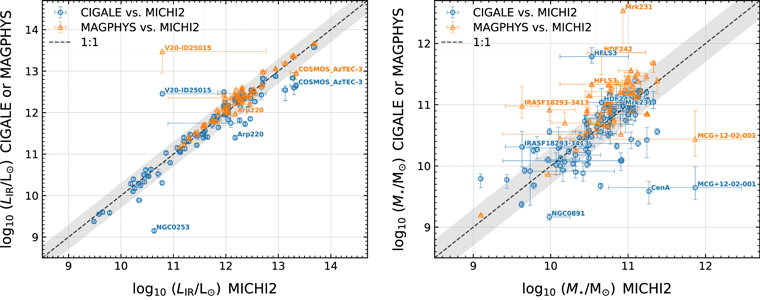
Figure 11. Comparison of the fitted 8–1000 μm dust luminosities (left panel) and stellar masses (right panel) from three SED fitting codes: MiChi2, CIGALE, and MAGPHYS. X-axes in both panels indicate the fitted parameters from the MiChi2, whereas Y-axes indicate those from either CIGALE (blue circles) or MAGPHYS (orange triangles). The dashed line is a one-to-one relation, and the gray shading indicates a ±0.3 dex range. Error bars show the fitted 16th and 84th percentiles, and symbols center at the minimum-χ2/highest-probability values.
Download figure:
Standard image High-resolution image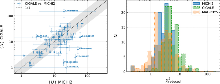
Figure 12. Left panel: comparison of the fitted  from MiChi2 and CIGALE. Symbols are similar to Figure 11, except that data points with reduced-χ2 > 10 are excluded. Right panel: histograms of the reduced-χ2 from MiChi2, CIGALE, and MAGPHYS SED fittings. Given that our fittings span from UV/optical to millimeter/radio wavelengths, a reduced-χ2 larger than unity is not unexpected. A value of a few still indicates a reasonable fitting in our cases, but >10 usually means poor or failed fitting.
Download figure:
Standard image High-resolution imageIn the comparison of  in Figure 12, we excluded the 12 sources with reduced-χ2 > 10 in CIGALE fitting. Although most sources have consistent
  , a small number of sources do not have consistent
  , and they mostly come from the V20 subsample. This is mainly because they have very poor IR photometry except for one or two submillimeter interferometry photometries. But we chose to skip these interferometry photometries in our CIGALE fitting tests owing to the filter setting. Adding a fake filter in CIGALE and rerunning the fitting for each of these sources are required in order to fit the submillimeter interferometry photometry, and then more consistent results are expected. Therefore, these comparisons show that for sources with good reduced-χ2 and photometry data MiChi2 and CIGALE have similar constraints on
  .
.
Appendix D: Gas Modeling Prediction on Line Optical Depth and [C i]/CO Line Ratio
We present the predicted [C i] (3
P1 − 3
P0) (hereafter [C i] (1–0)) and CO (1–0) line optical depths and the [C i] (1–0)/CO (1–0) line ratio in surface brightness unit ( ) in Figures 13–15. The optical depths shown in Figure 13 agree with normal conditions where CO (1–0) is optically thick, while [C i] (1–0) is roughly optically thin or has τ ∼ 1.
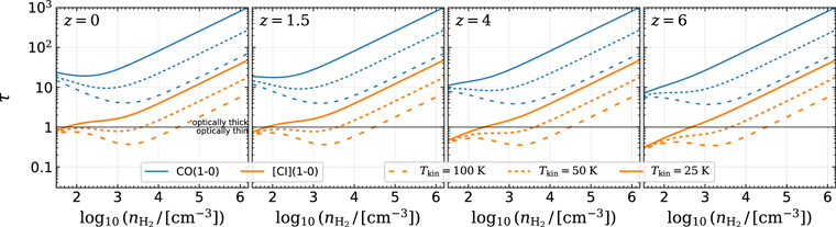
Figure 13. Optical depths (τ) of CO (1–0) and [C i] (1–0) as a function of the gas density of each single LVG (one-zone) model in four redshift panels. Blue lines are CO (1–0), and orange lines are [C i] (1–0). Line styles (solid, short-dashed, and long-dashed) represent different gas kinetic temperatures as labeled. These show that the derived optical depths from our models (Section 5) roughly agree with observations that usually show optically thin (τ ∼ 1) [C i] (1–0) and optically thick CO (1–0).
Download figure:
Standard image High-resolution image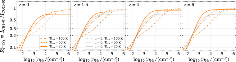
Figure 14. Ratio between [C i] (1–0) and CO (1–0) line surface brightness from our single LVG one-zone models. Lines and symbols are similar to those in Figure 4, but note that the ratio in Figure 4 is flux ratio while here we show the surface brightness ratio (}^{{\prime} }/{L}_{\mathrm{CO}(1-0)}^{{\prime} }$](https://content.cld.iop.org/journals/0004-637X/909/1/56/revision2/apjabd801ieqn457.gif) ).
).
Download figure:
Standard image High-resolution image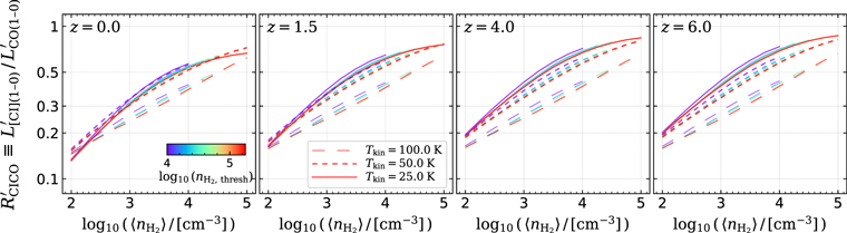
Figure 15. Ratio between [C i] (1–0) and CO (1–0) line surface brightness from our density–PDF gas modeling. Lines and symbols are similar to those in Figure 5 (see also the note about the different ratio definition in the caption of Figure 14).
Download figure:
Standard image High-resolution imageFigures 14 and 15 show  as a function of one-zone cloud molecular gas density and mean molecular gas density of the composite PDF, respectively. Similarly to Figures 4 and 5, we show our prediction at four redshifts, z = 0, 1.5, 4, and 6, and with three representative Tkin = 25, 50, and 100 K.
  increases with
  or
or  but strongly decreases with Tkin at intermediate
  . Future study of this line ratio with our gas modeling will shed light on how to better constrain Tkin and
  .
.
Footnotes
- 17
A Python package (co-excitation-gas-modeling) is provided with this paper for the calculation: https://pypi.org/project/co-excitation-gas-modeling. It fits an input line ratio with error to our model grid and determines the probable ranges of
and Tkin. - 18
A MySQL/MariaDB database is available for interested readers by request.
- 19
- 20
An SB galaxy is defined by its SFR being 4× greater than the MS SFR (e.g., the Speagle et al. 2014 equation) given its redshift and stellar mass. Vice versa, an MS galaxy is defined by its SFR being within 4× the MS SFR.
- 21
Their catalog is available at 10.5281/zenodo.3632388.
- 22
Their data are available at http://www.mpia.de/HERACLES/Overview.html.
- 23
Including Galaxy Evolution Explorer (GALEX) far-UV, near-UV, B, V, R, I, u, g, r, i, z, J, H, K, Spitzer/IRAC 3.6, 4.5, 5.8, 8.0 μm, Wide-field Infrared Survey Explorer 12 μm, Spitzer/MIPS 24 μm, Herschel/PACS 70, 100, 160 μm, Herschel/SPIRE 250, 350, 500 μm, and JCMT/SCUBA 850 μm. See their Table 2.
- 24
These are Mrk 231, NGC 0253, NGC 1365, NGC 2369, NGC 3256, NGC 4945, NGC 5135, NGC 7469, and NGC 7582. Note that we carefully selected photometric data with large-enough aperture to cover entire galaxies.
- 25
- 26
- 27
Their SED figures are accessible at the link mentioned in the caption of Figure 1. With high-S/N IRAC to MIPS 24 μm data, their mid-IR AGNs and any PAH feature if present can be well distinguished by our SED fitting. Yet we note that for galaxies with low-S/N IRAC to MIPS 24 μm data the uncertainty in AGN component identification could be high.
- 28
- 29
All SED fitting figures are available at 10.5281/zenodo.3958271.
