


Abstract
We report 1.2 mm polarized continuum emission observations carried out with the Atacama Large Millimeter/submillimeter Array toward the high-mass star formation region G5.89–0.39. The observations show a prominent 0.2 pc north–south filamentary structure. The ultracompact H ii region in G5.89–0.39 breaks the filament into two pieces. Its millimeter emission shows a dusty belt with a mass of 55–115 M⊙ and 4500 au in radius, surrounding an inner part comprising mostly ionized gas, with dust emission only accounting for about 30% of the total millimeter emission. We also found a lattice of convex arches that may be produced by dragged dust and gas from the explosive dispersal event involving the O5 Feldt's star. The north–south filament has a mass between 300 and 600 M⊙ and harbors a cluster of about 20 mm envelopes with a median size and mass of 1700 au and 1.5 M⊙, respectively, some of which are already forming protostars. We interpret the polarized emission in the filament as mainly coming from magnetically aligned dust grains. The polarization fraction is ∼4.4% in the filaments and 2.1% at the shell. The magnetic fields are along the North Filament and perpendicular to the South Filament. In the Central Shell, the magnetic fields are roughly radial in a ring surrounding the dusty belt between 4500 and 7500 au, similar to the pattern recently found in the surroundings of Orion BN/KL. This may be an independent observational signpost of explosive dispersal outflows and should be further investigated in other regions.
Export citation and abstract BibTeX RIS
1. Introduction
Similar to their low-mass counterparts, high-mass stars form inside molecular clouds that span across parsecs in size, typically adopt filamentary shapes, and can be seen as infrared dark clouds (IRDCs; Lis & Carlstrom 1994; Perault et al. 1996; Carey et al. 1998, 2000; Hill et al. 2005; Rathborne et al. 2006; Simon et al. 2006; Sanhueza et al. 2019). These filaments possibly originate by turbulence in the interstellar medium (ISM) imprinted at large scales by supernova explosions or high-speed massive-star winds (e.g., Inutsuka et al. 2015), among other phenomena (e.g., spiral density wave shocks, Parker and gravitational instabilities; Elmegreen 1990). Overdensities created within these structures fragment and collapse from dense cores down to 1000 au dusty envelope scales, which harbor the formation of freshly new stellar systems (e.g., Zhang et al. 2009; Bontemps et al. 2010; Zhang et al. 2015; Palau et al. 2020), most of which are multiple systems (e.g., Duchêne & Kraus 2013; Moe & Di Stefano 2017). It is well known that these young systems eject collimated winds or jets at velocities of 100–1000 km s−1, regulating the growth in the disk/envelope's angular momentum and allowing the accretion of gas and debris onto the protostars through rotating circumstellar disks (e.g., Cesaroni et al. 2007; Bally 2016). Some systems form objects several times more massive than the Sun and launch very powerful jets transferring huge amounts of kinetic energy into the environment via dragging and shocking the molecular material of the originally quiescent filamentary cloud (e.g., Beuther et al. 2002; Zhang et al. 2005; Qiu et al. 2008; López-Sepulcre et al. 2009; Fernández-López et al. 2013; Zapata et al. 2019a). Occasionally, gravitational interactions between the objects in these stellar systems can become chaotic. This occurs in systems with three or more objects orbiting each other. Some of these systems may end up with stars in very close orbits, which could contain colliding paths. In such occasions, it is plausible that the system is disintegrated, the individual disks tear into pieces, and, sometimes, even new objects could be formed from a violent merger (Bally & Zinnecker 2005; Bonnell & Bate 2005; Rodríguez et al. 2005).
The role played by the magnetic fields in each of the processes mentioned above is still not well understood because of the difficulty in their detection and measurement (but see Hull & Zhang 2019, for current ideas on this matter). The morphology of the field lines is also a difficult problem to solve since most of the time only a 2D projection in the plane of the sky can be inferred. Spinning grains preferentially align with their elongated dimension perpendicular to the field lines. Hence, the thermal millimeter and submillimeter emission from the grains is linearly polarized in a direction orthogonal to the magnetic field (see, e.g., Lazarian 1994; Cho & Lazarian 2007; Lazarian & Hoang 2007; Andersson et al. 2015). Specifically, the magnetic field inside interstellar medium (ISM) filaments has been studied at parsec scales using observations with the Planck satellite (e.g., Planck Collaboration et al. 2016a), revealing that in the densest filaments (like those forming the most massive stars in the Galaxy) the main direction of the magnetic field is generally perpendicular to their main direction (see also Pattle et al. 2017; Soam et al. 2019). Within the parsec-scale massive clumps where protoclusters are expected to form, spatially resolved observations revealed magnetic field configurations ranging from an hourglass-shaped morphology (e.g., G34.41+0.31, Girart et al. 2009; Beltrán et al. 2019; G240.31+0.07, Qiu et al. 2014) to a more random distribution (e.g., DR21(OH); Girart et al. 2013). However, a systematic submillimeter array (SMA) polarimetric study of 14 high-mass star-forming clumps found, on a statistical basis, that the magnetic field in dense cores tends to be aligned and perpendicular to the field of their parental clump (Zhang et al. 2014).
The ultracompact H ii region (UCHII) G5.89–0.39, also known as W28 A2, is a region that has probably formed (or it is forming) a new generation of massive stars (e.g., Zapata et al. 2019b, and references therein). Maser emission from several molecules has been spotted in the region (e.g., H2O, CH3OH, OH, NH3; Hofner & Churchwell 1996; Kurtz et al. 2004; Stark et al. 2007; Hunter et al. 2008). A huge amount of dense molecular material has been found surrounding the shell-like UCHII region, displaying hints of expansion motions (Gomez et al. 1991). Studying the ionized gas of the UCHII, Acord et al. (1998) derived that the H ii region is expanding at a velocity of 35 km s−1 and has a dynamical age of  yr. The gas in the UCHII region could be ionized by a young star with the luminosity of an O5V zero-age main-sequence star, identified by high angular resolution near-infrared observations, and lying at the northeast edge of the shell (Feldt et al. 2003). This star may have been at the center of the UCHII region 1000 yr ago if moving at about 10 km s−1. Puga et al. (2006) inferred the presence of a possible second young star in the northwest edge of the shell through the discovery of a possible Brγ ionized jet, but there is no direct evidence on the existence of such an object yet. Several extremely powerful outflows in different directions were reported in G5.89–0.39 (Harvey & Forveille 1988; Zijlstra et al. 1990; Sollins et al. 2004; Hunter et al. 2008). The kinetic energy of these ejections amounts to 1046–1048 erg, placing them among the most powerful outflows in the Galaxy. Very recently, tens of CO outflowing filaments have been found expanding from the center of the UCHII region, confirming the existence of a new explosive outflow (Zapata et al. 2019b, 2020). The discovery may imply that these kinds of events are much more frequent than previously thought (Zapata et al. 2020). In addition, possibly related to the event of an explosive outflow, G5.89–0.39 spatially matches with several high-energy sources from X-rays to TeV γ-rays, such as HESS J1800–240B (e.g., Gusdorf et al. 2015; Hampton et al. 2016). The TeV sources have been explained as the interaction between a population of cosmic rays accelerated in the supernova remnant W28 (located ∼1° north of G5.89–0.39) and the molecular envelope of the UCHII region (Montmerle 1979, 2017). However, shocks produced by the explosive event may be strong enough to accelerate particles up to the relativistic regime. Continuum millimeter and submillimeter observations carried out previously with the Submillimeter Array detected the dust associated with the edges of the UCHII region and the two north–south elongations (Sollins et al. 2004). These structures were later resolved into a dusty ring fitting the UCHII region and the emission from three additional sources to the north, east, and south (Hunter et al. 2008). Moreover, submillimeter polarized emission was detected toward a ridge of dust extending north–south across the western edge of the shell (Tang et al. 2009). These observations allowed us to set an upper limit to the magnetic field strength on the plane of the sky (<2–3 mG) and to conclude that the field-line morphologies are shaped by actors such as the radiation, pressure, and outflows of the region.
In this work we adopt a distance to G5.89–0.39 of  kpc estimated by Sato et al. (2014) after measuring the proper motions and infer the parallaxes of a group of 22 GHz H2O masers. However, a smaller distance of 1.28 kpc was obtained using the same technique (Motogi et al. 2011), and other works in the literature show a controversy with measurements between 1.3 and 7.0 kpc. In addition, the Gaia DR2 data inside a projected 3' ring centered at G5.89–0.39 show very large G-band extinctions (>1 mag at less than 1000 pc). This is possibly due to the proximity of this target with the direction of the Galactic center. Inspecting the Gaia DR2 data, it is not clear whether there are one or more clouds overlapped toward this line of sight. Actually, an analysis of the H i absorption line indicates a distance between 3 and 7 kpc (Zijlstra et al. 1990), and the stellar counting and extinction studies in red giants of Foster et al. (2012) both obtain distances between 3.5 and 4.5 kpc, closer to the distance found by Sato et al. (2014).
The present observations comprise deep 1.2 mm Atacama Large Millimeter/submillimeter Array (ALMA) polarization observations toward the G5.89–0.39 region. This target was observed as part of the Magnetic Fields in Massive Star-forming Regions (MagMaR) survey, which contains 30 sources in total. Details on the survey and source selection will be given in P. Sanhueza et al. (2021, in preparation). In Section 2, we describe the observations, along with 2 cm Very Large Array (VLA) archival observations. Section 3 shows the results, split into the raw continuum and the linear polarized emission at millimeter wavelengths. We discuss the results in Section 4 and summarize the main ideas in Section 5.
2. Observations
2.1. 252 GHz ALMA Data
Observations were conducted on 2018 September 25 using ALMA Band 6 (1.2 mm) under the MagMar project (code 2017.1.00101.S; PI: P. Sanhueza). A total of 47 antennas were used with baselines ranging between 15 and 1400 m. The precipitable water vapor (PWV) during the observations ranged between 1.1 and 1.4 mm, and the phase rms was below 0 31. The spectral setup contains five spectral windows: three of them (centered at 243.472, 245.472, and 257.472 GHz) are intended for continuum emission with a spectral resolution of 1.953 MHz (∼2.4 km s−1) and total bandwidth of 1.875 GHz each, while the other two are focused on resolving the H13CO+ (3−2) and HN13C (3−2) spectral lines with a spectral resolution of 488.281 kHz (0.56 km s−1) and bandwidth of 234.38 MHz. The continuum coverage was centered around 252 GHz with a total bandwidth of 5.8 GHz.
J1832−2039 was used as the phase calibrator, while J1924−2914 was adopted as the bandpass, the absolute flux scale, and the polarization calibrator. About 10% of absolute uncertainty in the flux calibration is expected for ALMA Band 6 observations. 18 Regarding the polarization uncertainty, the measured D-terms due to instrumental cross-talking between the two orthogonal polarized signals received (instrumental polarization) are less than 5%.
The observations toward G5.89–0.39 were intertwined with observations of six other scientific targets, which will be reported in future papers. The total time on source was 12 minutes. After the standard calibration, we selected only the line-free channels to make maps of the continuum emission. Continuum-only channels account for 72% of the total bandwidth available. We run three iterations of phase-only self-calibration, which improved the signal-to-noise ratio in the Stokes I image from 44 to 111. The images were Fourier-transformed, deconvolved, and restored using the CASA tclean task. The final Stokes I image has a synthesized beam of 0 29 × 022, PA = 841 (870 au × 660 au at the assumed distance), and an overall rms noise level of 1.1 mJy beam−1. For the Stokes Q, U, and V images the rms noise level is 0.04 mJy beam−1. We also build images of the debiased linear polarized intensity (
 ), the linear polarization fraction (pl
= ml
/I, average uncertainty of 0.6%), and the electric vector position angle (EVPA
), the linear polarization fraction (pl
= ml
/I, average uncertainty of 0.6%), and the electric vector position angle (EVPA  , average uncertainty of 6°).
The ALMA polarimetric capabilities for the Cycle 6 observations included full linear and circular operations for single pointing, with a field of view limited to the inner 1/3 and 1/10 of the primary beam, respectively (about 75 and 23 out of 229, at the observing frequency).
2.1.1. ALMA Circular Polarized Continuum Emission
At first glance, there appears to be a 5σ–10σ Stokes V detection in the ALMA data. The Stokes V spatial distribution is not coincident with the Stokes I emission. However, ALMA can sometimes create artificial Stokes V emission owing to its beam squint pattern. To determine whether this is a real signal, we made a simulated map of the ALMA beam squint pattern. We rotated it at the different parallactic angles covered by the observations and multiplied each resulting map by the Stokes I spatial distribution. We then Fourier-transformed each of these maps and concatenated all of them into a single file of visibilities. This file was then treated as the real visibilities observed by ALMA. The final cleaned image reproduced quite well the spatial distribution of the original Stokes V obtained from the ALMA observations, indicating that the 5σ–10σ detection is most likely spurious.
2.2. Ancillary 8.4 GHz VLA Data
The observations were made with the VLA of NRAO
19
centered at a rest frequency of 8.4 GHz (3.5 cm) during 1989 February. At that time the array was in its AB configuration. The observations used the 27 antennas of the array. The absolute amplitude calibrator was 3C 286, while the gain-phase calibrators were J1730−130 and J1741−038. The digital correlator of the VLA was configured in two spectral windows of 50 MHz. The data were analyzed in the standard manner using the AIPS package of NRAO. The resulting image rms noise and angular resolution are 82 μJy and 056 × 039, respectively, with a position angle of −875. The field of view is  .
.
3. Results
In this section we show the main results derived from the continuum ALMA observations toward G5.89–0.39. First, we present a description of the main features of the Stokes I continuum emission at 1.2 mm in this region, and second, we introduce the main linear polarization results.
3.1. 1.2 mm Stokes I Continuum Emission
Figures 1–5 show the overview of the millimeter emission toward G5.89–0.39, the comparison between the spatial distributions of the millimeter and centimeter emissions, the spectral index between both wavelengths, the location of the identified millimeter sources, and the detailed structure of the central part. We first address the large-scale structures in the images (see also Table 1), then we present the emission from the compact sources (Tables 2 and 3), and finally we identify the complex structures found at the center of the field of view.

Figure 1. 1.2 mm Stokes I continuum emission toward G5.89–0.39. The white symbol marks the position of the Feldt's star. The synthesized beam, in the lower left corner, is 029 × 022, PA = 841. The rms noise level of the image is estimated in 1.1 mJy beam−1.
Download figure:
Standard image High-resolution image
Figure 2. Zoom-in of the Central Shell structure. The 3.5 cm VLA continuum emission in contours (at 2, 6, 24, 72, and 100 times the rms noise level of 82 μm) is overlapped with the 1.2 mm ALMA continuum emission (color scale). The free–free ionized emission contribution at 1.2 mm toward the Central Shell is evidenced by the quite good overall spatial agreement of the emission at both wavelengths. That includes the inner shell's decrease of emission.
Download figure:
Standard image High-resolution image
Figure 3. Spectral index derived from the 3.5 cm VLA and the 1.2 mm ALMA continuum emission images. The VLA continuum emission is shown in contours at 2, 6, 24, 72, and 100 times the rms noise level. The spectral index α is estimated using Sν ∝ να .
Download figure:
Standard image High-resolution image
Figure 4. 1.2 mm Stokes I continuum emission toward G5.89–0.39. The three main regions (North and South Filaments and Central Shell) are marked along with the main dusty condensations associated with the Central Shell (S1–S18) and the dusty envelopes identified via dendrograms (MM1–MM23).
Download figure:
Standard image High-resolution image
Figure 5. Zoom-in of the 1.2 mm continuum emission of the Central Shell. A triangle marks the location we take as the center of the shell (ICRS 18:00:30.397, −24:04:01.4). The concentric circles of radii 08, 17, 32, and 54 demarcate the inner ionized region, the dusty belt, the ensemble of arches, and an outermost region with more faint arches and bow shocks. The rest of the symbols are the same as in Figure 4.
Download figure:
Standard image High-resolution imageTable 1. Masses of the G5.89–0.39 Large-scale Structures
| Zone | Flux | Td a | Mass a |
|---|---|---|---|
| (mJy) | (K) | ( M⊙) | |
| North Filament | 710 | 15/10 | 125/240 |
| Central Shell | 7488 b | 150/75 | 55/115 |
| South Filament | 820 | 15/10 | 145/275 |
Notes. The typical statistical uncertainties of the lower limit mass estimates due to the flux scale calibration are 10%. However, the dominant uncertainty in these mass lower limit measurements is the temperature uncertainty.
a Lower limit masses are derived assuming two different temperatures separated by a slash. b Total flux measured at 252 GHz in this work. We estimate that 2.959 Jy of this flux may be due to free–free emission and subtracted it to estimate the mass (see Section 3.1.1).Download table as: ASCIITypeset image
Table 2. Millimeter Envelopes in G5.89–0.39
| Source | R.A. | Decl. | Deconvolved Size | Peak Intensity | Flux Density | Mass |
|---|---|---|---|---|---|---|
| ICRS | ICRS | (arcsec × arcsec, deg) | (mJy beam−1) | (mJy) | ( M⊙) | |
| MM1 | 18:00:30.766 | −24:03:54.79 | 0.86 ± 0.04 × 0.38 ± 0.02, 70 ± 2 | 3.3 ± 0.1 | 20 ± 1 | 1.3/3.0 |
| MM2 a | 18:00:30.666 | −24:04:04.96 | 1.20 ± 0.07 × 0.49 ± 0.03, 65 ± 2 | 3.0 ± 0.2 | 31 ± 2 | 1.9/4.6 |
| MM3 | 18:00:30.639 | −24:03:56.87 | 1.79 ± 0.08 × 0.70 ± 0.03, 60 ± 2 | 2.7 ± 0.1 | 56 ± 2 | 3.5/8.3 |
| MM4/SMA-E a | 18:00:30.633 | −24:04:03.05 | 0.33 ± 0.04 × 0.22 ± 0.04, 144 ± 24 | 14 ± 1 | 34 ± 3 | 2.1/5.0 |
| MM5 a | 18:00:30.626 | −24:04:05.46 | 0.94 ± 0.04 × 0.25 ± 0.02, 39 ± 1 | 3.3 ± 0.1 | 18 ± 1 | 1.1/2.7 |
| MM6 | 18:00:30.612 | −24:03:55.42 | 0.43 ± 0.03 × 0.30 ± 0.02, 80 ± 8 | 6.5 ± 0.5 | 19 ± 1 | 1.2/2.8 |
| MM7 a | 18:00:30.598 | −24:04:00.31 | 0.46 ± 0.03 × 0.24 ± 0.02, 2.9 ± 0.1 | 8.2 ± 0.4 | 68 ± 4 | 4.3/10.0 |
| MM8 | 18:00:30.528 | −24:04:07.59 | 0.57 ± 0.05 × 0.34 ± 0.04, 32 ± 8 | 3.7 ± 0.2 | 16 ± 1 | 1.0/2.4 |
| MM9 | 18:00:30.509 | −24:03:57.35 | 0.90 ± 0.02 × 0.55 ± 0.01, 20 ± 2 | 7.4 ± 0.4 | 67 ± 1 | 4.2/9.9 |
| MM10/SMA-N | 18:00:30.495 | −24:03:58.76 | 1.1 ± 0.1 × 0.6 ± 0.06, 40 ± 5 | 10.0 ± 0.3 | 66 ± 2 | 4.1/9.7 |
| MM11 | 18:00:30.395 | −24:04:04.91 | 0.85 ± 0.03 × 0.81 ± 0.03, 179 ± 50 | 8.2 ± 0.4 | 75 ± 2 | 4.7/11.1 |
| MM12 | 18:00:30.385 | −24:04:05.96 | 0.75 ± 0.05 × 0.35 ± 0.03, 38 ± 4 | 3.0 ± 0.2 | 16 ± 1 | 1.0/2.4 |
| MM13 | 18:00:30.316 | −24:04:07.18 | 1.0 ± 0.04 × 0.66 ± 0.03, 178 ± 4 | 6.4 ± 0.2 | 74 ± 3 | 4.6/10.9 |
| MM14 | 18:00:30.293 | −24:04:11.84 | 0.23 ± 0.08 × 0.11 ± 0.09, 24 ± 33 | 4.1 ± 0.2 | 6 ± 1 | 0.4/0.9 |
| MM15/SMA-S | 18:00:30.285 | −24:04:04.87 | 0.60 ± 0.03 × 0.21 ± 0.02, 104 ± 2 | 47 ± 3 | 163 ± 7 | 10.2/24.1 |
| MM16 | 18:00:30.285 | −24:04:11.48 | 0.37 ± 0.04 × 0.16 ± 0.03, 55 ± 6 | 4.3 ± 0.2 | 8 ± 0.6 | 0.5/1.2 |
| MM17 | 18:00:30.278 | −24:04:10.45 | 0.71 ± 0.03 × 0.47 ± 0.02, 161 ± 5 | 4.2 ± 0.1 | 24 ± 1 | 1.5/3.5 |
| MM18 | 18:00:30.275 | −24:04:09.89 | 0.44 ± 0.01 × 0.33 ± 0.01, 125 ± 5 | 2.4 ± 0.1 | 8 ± 1 | 0.5/1.2 |
| MM19 | 18:00:30.272 | −24:04:06.60 | 1.04 ± 0.02 × 0.56 ± 0.01, 154 ± 1 | 4.4 ± 0.2 | 47 ± 1 | 2.9/6.9 |
| MM20 | 18:00:30.192 | −24:04:07.14 | 0.79 ± 0.02 × 0.67 ± 0.02, 110 ± 9 | 2.8 ± 0.1 | 26 ± 1 | 1.6/3.8 |
| MM21 | 18:00:30.178 | −24:04:07.80 | 0.68 ± 0.04 × 0.53 ± 0.04, 142 ± 12 | 2.5 ± 0.1 | 16 ± 1 | 1.0/2.4 |
| MM22 | 18:00:30.098 | −24:04:05.20 | 1.8 ± 0.1 × 0.79 ± 0.04, 77 ± 3 | 3.0 ± 0.2 | 68 ± 4 | 4.3/10.0 |
| MM23/SMA-W | 18:00:29.862 | −24:03:51.34 | 0.63 ± 0.02 × 0.51 ± 0.01, 85 ± 6 | 2.1 ± 0.1 | 13 ± 1 | 0.8/1.9 |
Notes. Masses estimated using dust temperatures 40 and 20 K are separated by a slash and presented in this order.
a Millimeter envelope possibly associated with the Central Shell but undetected in the VLA observations.Download table as: ASCIITypeset image
3.1.1. Large-scale Structure
Overall, the emission is in agreement with previous lower angular resolution millimeter observations (Hunter et al. 2008; Tang et al. 2009), but our observations reveal a lot more details. The most striking feature of the large-scale structure is the strong emission from the shell-shaped structure toward the central H ii region (Figure 1). The Central Shell matches the general resemblance of previous multiwavelength observations and the archival VLA 3.5 cm emission, thus confirming the good agreement between the spatial distributions of both centimeter and millimeter observations (Hunter et al. 2008). In fact, if we zoom in on the central structure (Figure 2) and overlay the VLA 3.5 cm contours, we see that part of the millimeter emission could be produced by free–free. The shell emission comprises various elongated condensations S1–S18 (identified using a dendrogram analysis, see Section 3.1.2 below, and marked as gray circles in Figures 2 and 4, see also Table 3). In particular, the peak emission at 1.2 mm in the whole region is located at S8 (123 mJy beam−1 or 37 K in brightness temperature, taking into account the beam size of the observations). As a reference point, let us mention that the O5 V star (hereafter the Feldt's star; Feldt et al. 2003) lies to the northeast of the structure (marked by a white star), close to the position of the S8 condensation. Up to the location of this condensation, the shell-like structure has a radius of about 15 (about 4500 au at the assumed distance) and shows an irregular shape, not smoothly circular, but more squared. The irregularity in the shape of the shell was noticed before by Puga et al. (2006).
Table 3. Condensations Associated with the Central Shell
| Source | R.A. | Decl. | S8.4 GHz | S252 GHz | α | Fraction of | Mass |
|---|---|---|---|---|---|---|---|
| ICRS | ICRS | (mJy) | (mJy) | Free–Free | ( M⊙) | ||
| S1 a | 18:00:30.555 | −24:04:01.64 | 41 | 64 | 0.1 | 0.38 | 0.6/1.2 |
| S2 a | 18:00:30.555 | −24:04:04.30 | 4 | 4 | 0.0 | 0.59 | 0.03/0.05 |
| S3 a | 18:00:30.531 | −24:04:03.53 | 56 | 65 | 0.0 | 0.51 | 0.5/1.0 |
| S4 | 18:00:30.520 | −24:04:02.05 | 98 | 162 | 0.1 | 0.36 | 1.6/3.2 |
| S5 | 18:00:30.499 | −24:04:02.41 | 42 | 72 | 0.2 | 0.35 | 0.7/1.5 |
| S6 | 18:00:30.478 | −24:04:00.57 | 61 | 106 | 0.2 | 0.34 | 1.0/2.2 |
| S7 a | 18:00:30.477 | −24:04:03.91 | 28 | 33 | 0.0 | 0.50 | 0.2/0.5 |
| S8 | 18:00:30.462 | −24:04:01.00 | 147 | 363 | 0.3 | 0.24 | 3.1/8.6 |
| S9 a | 18:00:30.434 | −24:04:03.25 | 33 | 27 | −0.1 | 0.72 | 0.1/0.2 |
| S10 | 18:00:30.420 | −24:03:59.62 | 69 | 114 | 0.1 | 0.36 | 1.1/2.3 |
| S11 b | 18:00:30.414 | −24:04:01.19 | 48 | 44 | −0.0 | 0.65 | 0.2/0.5 |
| S12 b | 18:00:30.411 | −24:04:01.87 | 45 | 52 | 0.0 | 0.51 | 0.4/0.8 |
| S13 | 18:00:30.403 | −24:04:02.58 | 255 | 670 | 0.3 | 0.23 | 7.7/16.1 |
| S14 b | 18:00:30.373 | −24:04:02.03 | 33 | 17 | −0.2 | 1.15 | ⋯ c |
| S15/SMA1 | 18:00:30.360 | −24:04:00.49 | 206 | 476 | 0.2 | 0.26 | 5.2/11.0 |
| S16 | 18:00:30.338 | −24:04:02.67 | 73 | 171 | 0.2 | 0.25 | 1.9/4.0 |
| S17/SMA2 | 18:00:30.324 | −24:04:01.95 | 197 | 691 | 0.4 | 0.17 | 8.6/17.9 |
| S18 | 18:00:30.296 | −24:04:01.36 | 88 | 221 | 0.3 | 0.24 | 2.5/5.3 |
Notes. Masses of the S-condensations in the shell are estimated after subtraction of a free–free contribution extrapolated from the 3.5 cm emission with a spectral index of α = −0.154. They are estimated using dust temperatures of 150 and 75 K, separated by a slash in the last column and presented in this order.
a Compact condensation external to the Central Shell. b Condensation which lies, in projection, inside the Central Shell. c Only ionized gas is found in this object at 1.2 mm.Download table as: ASCIITypeset image
As seen in Figure 1, a prominent filament of dust extends due northeast from the Central Shell (hereafter the North Filament). It bifurcates, and the northernmost tip forms a curved arch to the east. This filament has an approximate size of about 70 (0.10 pc) and covers a range of position angles between 25° and 40° (measured from the center of the Central Shell). The filament width, close to the Central Shell, is about 25, while farther north the west subfilament becomes narrower than 07 (about 2100 au).
Another filamentary structure extends also due south (the South Filament). It may well be the continuation of the North Filament if there were not an interruption by the Central Shell. The size of the South Filament is 82 (0.12 pc) with a position angle of 8° (measured from the center of the Central Shell), and, as in the North Filament, the ALMA image shows several millimeter sources along its extent.
We estimate the total gas and dust masses of the large-scale structures that we have identified so far: the North Filament, the South Filament, and the Central Shell. We assume optically thin isothermal dust emission and ignore the scattering opacity. Therefore, all the masses presented should be treated as well-informed lower limits. We use the relationship

where Fν
, d, κν
, and Bν
(Td
) are the total observed flux density, the distance, the grain opacity (which depends on frequency as  ), and the brightness of a blackbody at the dust temperature Td
, respectively. We choose β = 2.0, more appropriate for the dust of the ISM (Hildebrand 1983), resulting in κν
= 1.072 cm2 g−1 at the observing frequency and appropriate for dust with thin ice mantles and densities of 106 cm−3 (Ossenkopf & Henning 1994). We assume a gas-to-dust ratio of 100 for the calculation. We also choose a cold dust temperature of 10–15 K (Lee et al. 2014) for the filaments and 75–150 K for the Central Shell as discussed in Hunter et al. (2008). The masses of the North and South Filaments are 125 and 145 M⊙ when using Td
= 15 K (Table 1). For a 10 K temperature the derived masses are about a factor of two larger.
), and the brightness of a blackbody at the dust temperature Td
, respectively. We choose β = 2.0, more appropriate for the dust of the ISM (Hildebrand 1983), resulting in κν
= 1.072 cm2 g−1 at the observing frequency and appropriate for dust with thin ice mantles and densities of 106 cm−3 (Ossenkopf & Henning 1994). We assume a gas-to-dust ratio of 100 for the calculation. We also choose a cold dust temperature of 10–15 K (Lee et al. 2014) for the filaments and 75–150 K for the Central Shell as discussed in Hunter et al. (2008). The masses of the North and South Filaments are 125 and 145 M⊙ when using Td
= 15 K (Table 1). For a 10 K temperature the derived masses are about a factor of two larger.
Now, due to the contamination of free–free emission at millimeter wavelengths toward the Central Shell, we first need to subtract this contribution before calculating its total gas and dust mass. We follow the analogous estimate by Hunter et al. (2008) and adopt for the shell emission a uniform fiducial free–free radio spectral index of α = −0.154, adequate for the optically thin emission in G5.89–0.39 (here, Sν ∝ να ). The millimeter flux emission measured from the ALMA image at 252 GHz from the whole shell is 7.488 Jy, and from the VLA image at 8.4 GHz we extract a flux density of 4.992 Jy. The latter centimeter flux density, extrapolated using the fiducial value of α to 252 GHz, becomes 2.959 Jy. This amounts to 40% of the total flux measured at 252 GHz. The thermal dust emission at 252 GHz is therefore 4.529 Jy, resulting in a mass between 55 and 115 M⊙, depending on the dust temperature chosen. 20 Moreover, we analyze the emission from the Central Shell, splitting it in four different zones (see Figure 5): we first consider (i) an inner shell, and, increasing in radius from the center, (ii) a belt of strong continuum emission, and (iii) an external zone containing both an ensemble of arches and bow-shaped features, and, farther away, (iv) more wispy and diffuse emission from larger loops and arcs (see Figure 6). We estimate the actual measured spectral index of the three innermost zones using the VLA and ALMA observations (Figure 3). We also calculate their fraction of free–free emission at 252 GHz in the same manner as discussed above. In the inner shell, 77% of the emission comes from a gas with a spectral index consistent with that of an optically thin free–free ionized gas (α = −0.08; note, however, that measurements at three different wavelengths are needed to determine the opacity of the free–free emission), and we estimate that it contains 1.4/2.9 M⊙ of gas and dust mass. The dusty belt shows a rising spectral index (α = 0.18) suggesting 30% of free–free contamination. It contains 52–108 M⊙ of gas, the bulk of the mass of the Central Shell. Beyond the belt, in the external zone showing centimeter emission, the northwest and southeast protuberances show larger free–free contribution (∼67% and α = −0.04) than the east and west parts, which show 40% free–free contribution and a derived spectral index α = 0.10 (Figure 3). The gas mass content in this region amounts to 1.6/4.1 M⊙. Therefore, the free–free contamination is dominant in the emission from the inner zone and the northwest and southeast external protuberances. This emission is consistent with optically thin ionized gas. In the belt and the external east and west parts the emission is dominated by dust with a smaller free–free contamination.

Figure 6. Cartoon of the G5.89–0.39 star-forming region showing the different structures found in the ALMA 1.2 mm continuum emission, plus an idealized representation of the CO explosive dispersal outflow reported by Zapata et al. (2020).
Download figure:
Standard image High-resolution image3.1.2. Identification of Millimeter Envelopes and Dust Condensations
Using a dendrogram technique 21 (Rosolowsky et al. 2008), we have identified 22 mm envelopes 22 toward the filamentary structure of G5.89–0.39, 18 dust condensations 23 delineating the edge of the Central Shell or associated with it, and another envelope further northwest of the Central Shell (MM23), probably not linked with the main G5.89–0.39 structure. In the rest of this work we refer to dusty envelopes or just envelopes to name the sources only detected at millimeter wavelengths, while we use dust condensations or condensations to name the sources with a mixture of millimeter and centimeter emission. In Figure 4 the millimeter envelopes are marked with black crosses and the condensations with gray circles. The condensations show some degree of free–free contamination and are mainly detected toward the Central Shell emission.
Five envelopes are located along the North Filament, and 13 more are located along the South Filament (Table 2). In the North Filament the envelopes are spread out along the filament, separated by about 2'' between them. In the South Filament, the envelopes are crowded around three locations also separated by about 2'' between them: the surroundings of MM15, previously known as SMA-S (north part of the South Filament; Hunter et al. 2008), the surroundings of MM13 (middle part of the filament), and the surroundings of MM17 (southern tip of the filament). In addition, we identify four envelopes in the outskirts of the Central Shell that are possibly related to it (MM2, previously known as SMA-E, MM4, MM5, and MM7).
To estimate lower limits for the total gas and dust masses of the envelopes, we again assume that their emission is optically thin and isothermal, and we ignore scattering. We adopt a dust temperature between 20 and 40 K and a more appropriate β = 1.5 for dust in denser regions (see, e.g., Lee et al. 2014), resulting in a value of κν
= 1.026 cm2 g−1 at 1.2 mm (Ossenkopf & Henning 1994). Table 2 contains the estimations of the masses of all the millimeter envelopes in the region based on integrated flux densities from 2D Gaussian fits to their millimeter emission. Using Td
= 40 K, the masses range between 0.4 and 10.2 M⊙ with an average value of 2.4 M⊙ and a median of 1.5 M⊙ (masses are about a factor of two larger when considering the lower temperature of 20 K). The most massive envelope (MM15) is located 35 south of the center of the H ii region, and six other envelopes show intermediate masses of 3–5 M⊙ (MM3, MM7, MM9, MM10, MM13, and MM22).
Several condensations, observed at millimeter and centimeter wavelengths, demarcate the strongest emission from the Central Shell. We have identified 10 of them along the dusty belt; another three of them (S11, S12, and S14) within the shell; one (S1) southwest of it, within a small partially ionized gas arch; and four more (S2, S3, S7, and S9) associated with a prominent loop. The mass estimates of these condensations require a more careful treatment, since we first have to calculate the fraction of free–free emission at millimeter wavelengths for each of them. In this case we measure the flux density at both 8.4 and 252 GHz, integrating within boxes defined manually by following the millimeter spatial distribution of every source. Table 3 includes these fluxes along with calculated α spectral indices and the fraction of free–free contamination in the ALMA 1.2 mm, derived by extrapolating the centimeter emission (and using a spectral index of −0.154) for every source (Hunter et al. 2008; Tang et al. 2009). Only seven sources have a free–free contamination fraction over 0.50. These are the sources that lie both inside (S11, S12, and S14) and outside of the dusty belt of the shell (Figures 2 and 4), forming the southwestern prominent loop of ionized gas mentioned before (S2, S3, S7, and S9). In addition, all sources but two have a flat or slightly positive spectral index consistent with the model used by Hunter et al. (2008) of an H ii region with a frequency turnover below 30 GHz, plus a thermal dust emission component. S9 and S14 show, however, a negative spectral index, indicating that their millimeter emission mainly stems from pure ionized gas.
Using a dust temperature of 150 K, the derived masses of the condensations S1–S18 range between 0.03 and 8.6 M⊙ (Table 3), with mean and median values of 2.0 and 0.9 M⊙, respectively. We obtain a factor of two larger masses when using a lower temperature of 75 K.
3.1.3. Arches and Loops toward the Central Shell
The high angular resolution and the image fidelity of the ALMA observations reveal a complex system of substructures toward the location of the Central Shell. Zooming into this region (Figure 5), we can distinguish condensations, arches, and detailed morphology of the diffuse emission (with intensity levels of 1–4 mJy beam−1, which is between two and seven times 0.6 mJy beam−1, the local rms noise level in the outer shell zone), which reveal an intricate, structured, and complex bubble of ionized gas and dust.
The interior part of the shell-like structure (r < 08, with r measured from the center of the shell at ICRS 18:00:30.397, −24:04:01.4) mainly contains ionized gas (average spectral index −0.08, consistent with the optically thin regime) plus three condensations (S11, S12, and S14). Its bounds, demarcated by a dusty belt of stronger emission, are irregular and curved, more elongated in the east–west than the north–south direction. The belt (seen as a shell-like structure within 08 < r < 17) appears more four-sided than circular (see also Feldt et al. 2003). Moreover, the boundaries appear to be formed out of smaller and contiguous curved structures or arches. In spite of its irregularities, the boundary drawn by the ALMA 1.2 mm emission does not show any apparent break in its continuity surrounding the inner zone. Hunter et al. (2008) reported a break in the southwest part of the belt (seen at 875 μm and molecular emission), which is unseen in the ALMA data.
Immediately surrounding the belt, the ALMA emission reveals the presence of arches, many of which apparently present their tips oriented radially outward from the center of the shell structure. The ensemble of arches form a wispy pattern for radii in the range 17 < r < 32. In Section 4.6 we make an attempt at identifying some of these arches, which include the millimeter envelopes (MM2, MM4, MM5, and MM7) and condensations (S1, S2, S3, S7, and S9) reported here, but the limited contrast and sensitivity of the image hamper conclusive delineation of the structures. A few of these arches, blurred in coarser angular resolution observations, have been reported in the past as loops of ionized and molecular gas in G5.89–0.39 (Acord et al. 1998; Argon et al. 2000; Hunter et al. 2008), but the details of the new ALMA images allow one to disentangle their emission into substructures. In addition, we note here that in the northeast and southwest directions, roughly coinciding with the large-scale dust filament orientations, there are a smaller number of these arches.
At larger distances from the center of the shell (between 32 and 54) there are more faint arches of dust (Figure 5). The tips of these arches also appear oriented outward from the center of the shell, with position angles between 103° and 164° due southeast, and between −77° and −16° for their corresponding northwest counterparts.
3.2. 1.2 mm Linear Polarized Continuum Emission
3.2.1. Overview
The 1.2 mm linear polarized intensity (ml ) spreads over the three characteristic regions in G5.89–0.39 (left panel of Figure 7). It peaks at the MM15/SMA-S envelope (ml = 1.10 mJy beam−1) and shows a relatively strong southwest–northeast ridge along the North Filament (especially near MM9) and the western half of the Central Shell. We note that most of the polarized emission toward the Central Shell does not exactly coincide with the location of the brightest Stokes I emission from the belt. The area more polarized is instead shifted toward the exterior of the belt, as if it were surrounding the western half of the belt. Overall, the linearly polarized emission covers large areas of the North Filament and the north and west parts of the Central Shell. On the South Filament the polarized emission is more scarce, and it is mainly distributed in the surroundings of some millimeter envelopes such as MM15, MM13, MM14, and MM16 at the southernmost tip.

Figure 7. Left: linearly polarized intensity overlapped with 1.2 mm continuum emission contours at 1, 4, 40, and 100 times the rms noise level of 1.1 mJy beam−1. Figure 10. Right: polarization fraction overlapped with continuum emission contours (same as left panel).
Download figure:
Standard image High-resolution imageThe spatial distribution of the linear polarization fraction (pl ; right panel of Figure 7) shows an evident difference between the Central Shell region and the filaments. While pl is on average about 4.3%–4.4% in the North and South Filaments, with peaks well over 10% at some specific locations (see also Figure 8), it drops down to 0.8% on average in the Central Shell, mainly detected in its western part. The sudden drop in the polarization fraction toward the Central Shell cannot be explained totally by the contribution of the free–free emission at 1.2 mm, since, as indicated in Tang et al. (2009), free–free emission is completely unpolarized. That is, while the linear polarized emission is only due to dust, the Stokes I intensity has an additional contribution from free–free, thus contaminating (i.e., decreasing the value) the polarization fraction of the polarized dust emission (since the Stokes I emission produced by the dust would be lower, the dust polarization fraction should be larger than the measured value). On average, we estimated that ∼40% of the continuum emission at 1.2 mm in the Central Shell is due to free–free emission; removing the effect of free–free emission in the Stokes I intensity, this would result in a factor of a few larger polarization fraction on average over this region. Hence, this correction does not change the fact that there is a sudden drop of pl over the Central Shell (0.8% becomes 2.1%); it just indicates that the decrease is not as extreme. Figure 9 shows the radial distribution of polarization fraction after removing the free–free unpolarized emission 24 from the Stokes I toward the Central Shell in more detail. It shows a gradual decrease in the polarization fraction at around the dusty belt position even accounting for free–free contamination (yellow bands). The corrected polarization fraction decreases from ∼4.0% in the outer shell down to ∼0.3% in the dusty belt. From the dusty belt inward, the polarization fraction suddenly increases again to an average value of ∼2.6%.

Figure 8. Free–free corrected polarization fraction vs. free–free corrected Stokes I intensity in G5.89–0.39. A power-law trend with a slope of −0.72 was found when fitting the data with Stokes I over a 3σ threshold.
Download figure:
Standard image High-resolution image
Figure 9. Free–free corrected polarization fraction as a function of the distance from the shell center (ICRS 18:00:30.397, −24:04:01.4). The color code shows stronger Stokes I emission in red circles and weaker emission in blue circles. Fitted power-law functions to the data of each zone of the Central Shell appear in dotted black curves highlighted in yellow bands.
Download figure:
Standard image High-resolution imageFigure 8 presents the relationship between the free–free corrected polarization fraction pl and the free–free corrected Stokes I intensity (also known as the P-I relationship) in the whole region. The data can be fitted by a power law with a slope s = − 0.722 ± 0.004 (pl ∝ Is ), close to unity, indicating that the polarized intensity scales like the Stokes I intensity (see also Tang et al. 2009). This is usually interpreted as the polarized intensity being produced in a surface layer of the molecular cloud and attributed to grains aligned by radiation torques (e.g., Kwon et al. 2019; Pattle et al. 2019). However, the scatter at each Stokes I intensity (of up to one order of magnitude, e.g., from 0.7% to 7% at 10 mJy beam−1) still leaves the door open to different possibilities or trends at particular, smaller locations. The simple anticorrelation trend is probably not capturing all the essential physics of the polarized emission. Moreover, there are some departures from the anticorrelation trend at Stokes I intensities of 10–11 mJy beam−1 and 50–100 mJy beam−1. These departures may indicate more complicated scenarios (see, e.g., Section 3.2.2 below).
Figures 10 and 11 show the spatial distributions of the EVPA and the inferred magnetic field orientations, respectively. To derive the magnetic field orientations, we assume that these are orthogonal to the linear polarization orientations of EVPA, as expected for grains aligned magnetically. From now on, we comment on the magnetic field orientations unless otherwise noted.

Figure 10. EVPAs overlapped onto the Stokes I continuum emission toward G5.89–0.39. Black/white segments indicate that the polarization percentage is below/above 2% (no free–free correction applied to this image). A segment is displayed approximately per every beam, using data with a 2σ cut in the debiasing process (same as in Figure 7). Contours are displayed at 1, 4, 40, and 100 times the rms noise level of 1.1 mJy beam−1.
Download figure:
Standard image High-resolution image
Figure 11. Same as Figure 7, but with the EVPAs rotated by 90° to show the inferred magnetic field morphology.
Download figure:
Standard image High-resolution imageThe North Filament shows a striking alignment of the magnetic field along its major axis (average PA of 54°; Figure 12), even accounting for the small turn of its northern tip, with a slightly different orientation from the rest of the filament. This can be easily seen in the histogram in panel (a) of Figure 12, which shows a peak of magnetic field orientations close to the main filament orientation, with local angles between 35° and 50°, and also in agreement with the northern tip orientation of 74°. Similar magnetic field alignment was found for the filament-like streamers in the IRAS 16293–2422 region (Sadavoy et al. 2018).

Figure 12. Histogram of magnetic field orientations toward each one of the three main regions identified in Figure 4. (a) The vertical red dotted lines mark the orientation of the North Filament (between 35° and 50°) and its northern tip ridge (at PA = 74°). (b) Central Shell histogram. (c) The vertical red dotted line marks the average orientation of the South Filament at −45. Both histograms for the northern and southern filaments (panels (a) and (c)) show clear single-peaked distributions.
Download figure:
Standard image High-resolution imageAt the location of the Central Shell, the magnetic field distribution seems more chaotic at first glance, but a more careful inspection leads us to see that it is mostly radial beyond the belt of dust. Panel (b) of Figure 12 shows a more homogeneous distribution of the magnetic field orientations toward the whole H ii region than in the filaments. This may be in accordance with the expectations for either radial or azimuthal distributions. However, when considering the magnetic field orientations in an annular region surrounding the dusty belt (15 < r < 25), the magnetic field shows a rough consistency with a radial pattern (Figure 13).

Figure 13. Residuals (absolute value of the difference) between the magnetic field orientations and a radial field distribution plot as a function of the position angle measured with respect to the center of the Central Shell (ICRS 18:00:30.397, −24:04:01.4), for pixels at radii between 15 and 25. For the position angles, 0° points north and + 90° points east. Difference residuals close to zero indicate a good agreement with a radial pattern for the magnetic field. Note the excursion of the data away from the radial pattern in the northwest quadrant (around −45°), likely due to polarized emission related to the dusty belt. Excluding these data, the median and standard deviation of the residuals are 22° and 14°, respectively.
Download figure:
Standard image High-resolution imageIn the South Filament, the magnetic field segments follow a simpler distribution close to MM15, with an average orientation of 89°, tracing the east–west elongation of the dust surrounding this envelope. This pattern is pinched at the very position of MM15 (see Section 3.2.2). Otherwise, the polarization measurements are more scarce in the rest of this filament, with an average orientation of 88°, which is almost perpendicular to the orientation of the filament itself (with local orientations typically of −45). The magnetic fields around MM8 and MM21 change the orientation abruptly, while at MM14 and MM16 they follow an east–west orientation, perpendicular to the filament.
3.2.2. Polarization toward the MM15 Millimeter Envelope
Table 4 summarizes the polarization properties toward some of the compact millimeter envelopes in which polarized emission is sufficiently detected (i.e., more than a beam size area with polarized emission). An interesting case corresponds to the brightest of them, MM15, which shows a pl peak of 4.1%.
Table 4. Measurements on the Polarization Maps
| Zone | ml ( mJy beam−1) | pl (%) | EVPA (deg) | ||||
|---|---|---|---|---|---|---|---|
| F | P | Mean | P | Mean | Mean | σ | |
| MM1 | 0.06 | 0.12 | 0.10 | 6.4 | 3.6 | −61 | 14 |
| MM3 | 0.15 | 0.20 | 0.12 | 8.1 | 5.0 | −20 | 17 |
| MM4 | 0.30 | 0.18 | 0.12 | 3.7 | 1.8 | 86 | 78 |
| MM5 | 0.28 | 0.17 | 0.12 | 6.3 | 4.4 | −11 | 11 |
| MM9 | 0.40 | 0.39 | 0.21 | 5.7 | 3.2 | −53 | 6 |
| MM10 | 0.27 | 0.27 | 0.20 | 3.0 | 2.1 | −62 | 7 |
| MM13 | 0.23 | 0.16 | 0.11 | 3.3 | 2.3 | −21 | 15 |
| MM14 | 0.32 | 0.36 | 0.20 | 18.6 | 8.6 | −11 | 5 |
| MM15 | 1.58 | 1.10 | 0.32 | 4.1 | 1.4 | −66 | 46 |
| MM16 | 0.51 | 0.36 | 0.18 | 14.1 | 7.7 | −28 | 11 |
| MM23 | 0.58 | 0.23 | 0.16 | 12.6 | 9.7 | −67 | 6 |
Note. ml is the linear polarized intensity in mJy beam−1; pl is the degree of linear polarization (in %); EVPA is the electric vector position angle (in degrees). F designates the integrated flux, P designates the peak intensity value, Mean is a measure of the mean value, and σ is the standard deviation taken over the pixels inside manually defined boxes for every source. Angle values were extracted using directly averaged values on Stokes Q and U images.
Download table as: ASCIITypeset image
Figure 14 presents two panels with a zoom-in view of the MM15 surroundings. The left panel shows the centrally peaked distribution of the polarization intensity along with the magnetic field orientation. The right panel shows the spatial distribution of the polarization fraction with a local maximum (pl
= 2.4%) slightly offset from the continuum peak position ∼01 west, surrounded by a ring of low polarization fraction (pl
≃ 1%), which is likewise embedded in a region of emission with high polarization fraction (pl
≃ 7%).

Figure 14. Left: linearly polarized intensity overlapped with continuum emission contours toward MM15. Segments show the magnetic field orientations. Right: polarization fraction overlapped with continuum emission contours toward the MM15 millimeter envelope (also known as SMA-S). Contours of the continuum emission in both panels are at 3, 5, 10, and 15 times the rms noise level (1.1 mJy beam−1). The synthesized beam is included in the lower right corner. A white cross marks the position of the Stokes I peak emission.
Download figure:
Standard image High-resolution imageIn general, the magnetic field distribution toward MM15 roughly follows the east–west elongation of the dust emission. However, close to the continuum peak, the orientation of the magnetic field segments has a dramatic ∼ 90° jump (Figure 14).
Figure 15 presents the P-I relationship in the neighborhood of MM15. The data can be clearly divided into two regimes. We fit the data with Stokes I emission between 3.3 and 17 mJy beam−1 with a power law with a slope s = −1.1 ± 0.1. For the data over 17 mJy beam−1, despite the larger scatter, a power-law fit gives a slope of s = 0.6 ± 0.2. A negative/positive slope in the P-I plot indicates lower/higher efficiency in polarization at higher dust densities.
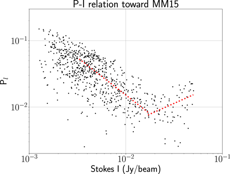
Figure 15. P-I relation toward the MM15 millimeter envelope. Two linear trends are plotted for Stokes I intervals between 3.3 and 17 mJy beam−1 and >17 mJy beam−1, respectively.
Download figure:
Standard image High-resolution image4. Discussion
4.1. General Scenario for the Star Formation in G5.89–0.39
The presented 1.2 mm ALMA continuum observations toward G5.89–0.39 revealed a filamentary structure about 18'' long (∼0.25 pc), interrupted by the well-known ionized shell-like structure at its center that hosts an extremely energetic explosive outflow (Zapata et al. 2019b, 2020). We propose here a scenario in which the North and South Filaments were part of the same molecular cloud structure. They were possibly part of a single curved filamentary cloud, hosting a small cluster of intermediate- and high-mass protostars at the position where we now see the center of the Central Shell. This central cluster may have formed an unstable multiple system that finally unleashed an explosive dispersal event (as it seems to have occurred in the Orion BN/KL system; Bally & Zinnecker 2005; Rodríguez et al. 2005), driving gas and dust debris outward quasi-isotropically at high velocities. After the explosive dispersal event, the H ii region (which may or may not have existed before the blast) includes hot ionized H ii gas mixed with warm dust; the latter is mainly concentrated in the aforementioned ∼4500 au radius projected belt-like structure. Possibly embedded in this dusty belt is the only stellar object confirmed to date: the O5 Feldt's star, probably the main ionizing source. However, there also is evidence for another star as identified by Puga et al. (2006), using a velocity gradient attributed to its outflow. The outflows from the protocluster members, the expanding UCHII region, and the explosive dispersal event may have shaped the environment until getting the present shell-like appearance. Furthermore, there is reasonable evidence that the ejected gas and debris are probably reaching some of the more nearby star formation centers, such as MM15 (e.g., see SiO molecular images in Zapata et al. 2020).
In more remote places of the molecular cloud/filament, the ongoing process of filament fragmentation is probably unaffected by the explosive event, as the shock wave has not yet reached these areas. In these locations, several envelopes have already gravitationally condensed, creating protostars revealed by the millimeter emission from dust and the presence of collimated outflows (such as MM1 and MM6, which are associated with collimated bipolar outflows seen in 12CO, which we will show in a forthcoming publication). While the fragmentation process has not disrupted the overall structure of the North Filament (note, however, that it diverges into two subfilaments), the South Filament is more patchy, with three local star formation centers associated with the millimeter envelopes MM13, MM15, and MM17. Nonetheless, the filamentary nature of the South Filament can be perceived in the almost north–south alignment of several of its envelopes, while still preserving the original large-scale structure.
4.2. Orientation of the Polarized Emission in the Central Shell
The main morphology distribution of the linear polarization EVPAs (i.e., not rotated to show the inferred B-field) in the Central Shell, the azimuthal polarization pattern beyond the dusty belt (Figure 10), may be explained by emitting dust grains aligned with the radial magnetic field (Lazarian 1994; Cho & Lazarian 2007; Lazarian & Hoang 2007). We assume this explanation in Section 3, but we discuss here whether this distribution could possibly also be explained by the alignment via radiative flux (e.g., Tazaki et al. 2017) coming from the center of the explosion as a locally anisotropic flow of photons, or even by a process of self-scattering provided by anisotropic thermal dust emission (Kataoka et al. 2015; Yang et al. 2016). These last two alignment mechanisms need dust grains with sizes of about λ/2π (∼0.2 mm), which seems implausible, for typical interstellar dust grains are micron sized. Additionally, a scenario with grains aligned mechanically by an isotropically expanding blast has to be rejected in principle, because the grains will be oriented radially and will produce a radial polarization pattern (Gold 1952), opposite to the azimuthal one encountered in the ALMA images. However, the alignment via mechanical torques (e.g., Hoang et al. 2018) may explain the radial distribution of the magnetic field. In addition, a similar azimuthal pattern has been observed up to ∼4500 au from the center of the explosive dispersal outflow in Orion BN/KL (e.g., Cortes et al. 2020). The mechanical alignment of grains was claimed to explain sudden changes in the orientation of the polarization at larger scales in this region (Rao et al. 1998), but Tang et al. (2010) and Cortes et al. (2020) favored the magnetic alignment scenario to explain the millimeter polarized emission. Furthermore, they estimate that the explosive outflow may be energetic enough to drag the magnetic field lines, and they arrange them into the observed radial pattern. Assuming that both explosive events produce similar outcomes, we also favor the scenario of magnetically aligned grains in the Central Shell of G5.89–0.39 as the main contributor to the millimeter polarized emission.
The present ALMA observations toward G5.89–0.39 show polarized emission at the belt of dust emission but primarily outside it, in the less dense parts of the Central Shell (Figure 11). The polarized emission is more likely found in the western hemisphere of the shell. Along the dusty belt, the orientation of the magnetic field segments is irregular, although many appear to be azimuthal with respect to the center of the shell, especially at the location of the millimeter condensations (Figure 11). Beyond the dusty belt, the orientation of the magnetic field is predominantly radial (Figures 10 and 13). The polarization percentages decrease progressively inward down to the inner boundary of the dusty belt (Figure 9). From that point to the the center of the shell, the polarization fraction increases again. This can be another manifestation of the "polarization hole," where the polarization fraction gets lower as Stokes I emission gets higher owing to preferential alignment at a surface layer of the dusty belt or to depolarization effects (see also Section 4.5). In this case, the sudden change on the magnetic field orientation at the outer edge of the dusty belt may be connected to the polarization fraction drop (e.g., due to tangled up magnetic fields), which can raise the question of whether the field lines are being reshaped owing to the ionization and/or the expansion of the shell. What is clear is that a radial distribution does not correspond to the idealized models of expansion of bubbles through uniform magnetic fields (e.g., Ferriere et al. 1991). One possible scenario is that during the first stages of the explosion the compression on the dusty belt made the fields azimuthal. In more evolved stages, at the position of the condensations in the belt (zones of maximum compression), the magnetic field resistance against the expanding wave is maximal, acting as stagnation points where the gas ram pressure and the thermal pressure are balanced by the magnetic field tension. If magnetic fields are flux-frozen to the gas, they will be dragged along, with the outgoing motions creating an outward radial magnetic field pattern.
In any case, finding a prevailing radial magnetic field accompanying the explosive dispersal toward G5.89–0.39 (Zapata et al. 2019b, 2020) makes two such systems with the same magnetic field signpost (the other being Orion BN/KL; Cortes et al. 2020), which are unique in detecting the relation between the feedback event and its fields. This signpost (more difficult to detect in low angular resolution observations and/or at older evolutionary stages; Planck Collaboration et al. 2016b; Soler et al. 2017) should be tested in other explosive dispersal candidates, as it could be an independent way of corroborating the existence of these special protostellar outflows.
4.3. Analogous Magnetic Field Morphology in Supernova Remnants
In G5.89–0.39, the shell comprises both ionized gas and dust, and it is thought to expand at ∼35 km s−1 (Afflerbach et al. 1996; Acord et al. 1998). This is reminiscent of the shells created by planetary nebulae, supernova remnants (Gomez et al. 1991), or even superbubbles (Ferriere et al. 1991), whereas in this case the shell is at the center of an ISM filament showing an incipient star formation process, and thus it is at a very young stage. Furthermore, we note here that the physics of the expansion of an H ii region is different from that of a supernova remnant, and the primary source of radio emission in supernova remnants is synchrotron emission, characterized by a negative spectral index and an expected large degree of linear polarization at centimeter wavelengths. Although the basic model of an expanding bubble may explain the overall physics in G5.89–0.39, the escape of hot gas and winds are significant effects (Geen et al. 2020), not clearly established in this region. None of these have been observed toward G5.89–0.39 (Afflerbach et al. 1996; Sollins et al. 2004; Hunter et al. 2008; Tang et al. 2009). Nonetheless, we find similarities between the distribution of the magnetic fields in G5.89–0.39 and those found in supernova remnants, which may be interesting to explore (such as Cas A; see Dunne et al. 2009).
In their review, Dubner & Giacani (2015) comment that the magnetic field orientation in supernova remnants may depend on their age. Young shell-type remnants present a radial distribution of magnetic fields, whereas in older remnants the distribution is predominantly parallel to the front shock or is tangled (Milne 1987). The origin of the radial distribution at the interface between the expanding front of young remnants and the swept-up environment could be produced with the amplification of the fields by the stretching of Rayleigh–Taylor instabilities in the mixing layer (e.g., Jun & Norman 1996), but this is still a matter of debate (see, e.g., West et al. 2017, for an alternative model).
Nevertheless, the conclusion is that synchrotron polarized emission from supernova remnants is oriented orthogonal to the magnetic fields, as with the magnetically aligned grain case. If the polarization at millimeter wavelengths is produced by a mechanism related to the magnetic fields (grain alignment or synchrotron emission), the orientation of the EVPAs would be expected to be perpendicular to the field lines. Hence, the magnetic field lines would be predominantly radial, as observed in G5.89–0.39. The possibility that the explosive event in G5.89–0.39 somehow produced particles accelerated up to relativistic velocities and created a small population of synchrotronic plasma seems unlikely at first glance. However, this scenario would be supported by the detection of high-energy sources (from X-rays to γ-rays; see, e.g., Gusdorf et al. 2015, for a summary) matching the position of G5.89–0.39 (Hampton et al. 2016), although the usual explanation for the HESS source is that it is produced by the interactions of cosmic rays accelerated in the northern W28A2 supernova remnant with the dense gas of the star formation region.
More detailed observational work is needed (multiwavelength deeper images) to disentangle the different contributions to the emission (thermal dust, thermal free–free, and possible nonthermal synchrotron emission) to extract more information about the physical conditions of the gas and dust in the region. This will help us to obtain a better informed interpretation of the explosive event and its interaction with the previous outflow ejecta and the possible preexisting H ii region.
4.4. Orientation of the Polarized Emission in the Filaments
In most regions of the ISM, it is usually assumed that dust grains are aligned with their long axis perpendicular to the magnetic field lines through the effect of radiative torques (RATs; Draine & Weingartner 1996; Lazarian & Hoang 2007, 2008, 2019; Hoang & Lazarian 2008, 2009, 2016). Here, we presume that this is the situation in most of the North and South Filaments.
Observations with the Planck satellite (Planck Collaboration et al. 2016a) have revealed that elongations of gas with column densities below 5 × 1021 cm−2 in the diffuse ISM are predominantly aligned with their associated magnetic fields, while more dense filaments (column densities over 5 × 1021 cm−2) are found to be mostly perpendicular to the magnetic fields (Hennebelle & Inutsuka 2019, and references therein). In G5.89–0.39, the ALMA polarization observations show that the elongation axis of the North Filament is mostly aligned with the magnetic fields, and the South filament is perpendicular to them. 25 The average column density for both filaments is similarly high (even taking into account their lower derived masses, we obtain values higher than ∼1024 cm−2), both lying in the high-density regime in which the filaments are expected to be perpendicular to the magnetic fields. The North Filament does not comply with this expectation. One possible explanation is that the magnetic fields, although orthogonal to the filament, are contained in a plane perpendicular to the plane of the sky, and therefore we would see their projection as aligned with the filament orientation. Doi et al. (2020) estimate that the probability of this special 3D-spatial configuration for filaments with orthogonal magnetic fields is 14% (allowing a 30° separation from the perpendicularity of the plane containing the magnetic fields and the plane of the sky). Hence, this configuration has low probability. Another explanation may come from the theoretical predictions for weakly magnetized filaments. For these, turbulent motions and gravity largely dominate the energy budget. Soler et al. (2013) have found that for weakly magnetized filaments, even in the case of large densities, the magnetic field may be predominantly aligned with the filament (see also Hennebelle & Inutsuka 2019). For G5.89–0.39, this may be the case for the North Filament, while the magnetic fields may play a different, more active role in the energy budget of the South Filament. Soler & Hennebelle (2017) have found, in addition, that both aligned and perpendicular configurations between magnetic field and filament orientation may be preferred configurations in numerical simulations. The perpendicular configuration may only be seen in converging flows threaded by more prominent magnetic fields. In addition, given an initial magnetic field strength and high enough density, switching between both configurations may be triggered by compressive motions.
In any case, G5.89–0.39 is a challenge for both hypotheses, since the North and South Filaments may be possibly part of the same structure (apparent continuous north–south morphology) and present two separate magnetic field distributions. The reason behind the magnetic field differences between the North and South Filaments is thus unclear. It could be related to intrinsic orientation (projected geometry of the filaments) or strength changes in the magnetic field. The latter could likewise be related to differences in the star formation evolutionary stage of the envelopes embedded in both filaments. For instance, the South Filament could be more advanced in terms of gravitational fragmentation and collapse, as indicated by the many local centers of star formation. Figure 12 shows that, close to the main millimeter envelopes, the magnetic field lines are pinched and present a lower polarization fraction. This could indicate that the field-line geometry is dominated by gravitational processes, hence explaining their different orientations with respect to those in the North Filament.
An alternative scenario may involve a strong interaction of the explosive outflow with the South Filament and a milder interaction with the North Filament, which may be somehow shielded because of the geometry and dust density distribution of the system. There is evidence showing the probable impact of some explosive outflowing filaments against the dust pocket surrounding MM15 (Zapata et al. 2020). The north side of this pocket shows magnetic field lines mainly oriented in the east–west direction, whereas there are a few segments in the southern side aligned in the northeast–southwest direction. In this scenario, the east–west orientation of the field lines (roughly orthogonal to a vector from the shell center) may be the product of compression due to shocks at the northern border of the dust pocket, as in MM2 and MM5. This may also be the case for the surrounding dust of other envelopes such as MM13 and MM22, although more evidence should be gathered. Regardless of this alternative scenario, the fact that we stress in this section is that in the filamentary structure of G5.89–0.39 the magnetic fields experience abrupt orientation changes between the North and South Filaments.
4.5. Linear Polarization toward MM15
At >2000 au spatial scales, the magnetic field spatial distribution around MM15 seems to follow a uniform orientation roughly in the east–west direction (Figure 14). This direction is perpendicular to the South Filament orientation, but it is also locally perpendicular to the explosive outflow from the Central Shell. Hence, it is difficult to decide whether the field orientation is due to the perpendicular accretion flows channeled into the South Filament or a process of compression due to the explosive dispersal outflow.
At <2000 au spatial scales, toward the center of the MM15 millimeter envelope, the magnetic field orientation jumps from the east–west to a more north–south direction. This is reminiscent of the expectations for a magnetically regulated collapse (e.g., Girart et al. 2006, 2009; Stephens et al. 2013; Maury et al. 2018; Kwon et al. 2019), where the initially uniform distributed magnetic field lines are mainly distributed along the rotation axis of the system, but dragged and pinched as the collapse advances. The MM15 envelope is elongated in the east–west direction, which may indicate that its rotation axis is north–south, coincident with the field lines at the center of the envelope. Higher angular resolution observations are needed to support this interpretation.
In addition, we report an overall linear decrease of the polarization fraction as the Stokes I intensity increases up to 17 mJy beam−1 (Figure 15). This behavior (the so-called "polarization hole") has already been seen in many other star-forming regions, and it is usually interpreted in two ways (e.g., Soam et al. 2018; Le Gouellec et al. 2019, 2020; Pattle et al. 2019; Kwon et al. 2019; Planck Collaboration et al. 2020). First, it can indicate the detection of the polarized emission produced by the magnetic alignment via radiative torques due to interstellar photons in a surface layer of the cloud. This would mean that the grains are aligned with the magnetic fields only in the outer skin of the cloud. Second, it can indicate several depolarization effects. These can be caused by unresolved magnetic field structure within the beam, grain growth in denser regions (and hence less alignment due to the more spherical shape of the larger grains in these regions), collisional de-alignment of grains in high-density regions, destruction of grains via RAT-D (Hoang et al. 2019), or a lower flux of photons due to higher optical depth close to young stars. In the case of MM15, we have also detected a different pattern closer to the millimeter envelope peak emission (Figures 14 and 15). Over 17 mJy beam−1 (marked approximately by the 15σ contour in Figure 14) the polarization fraction increases with Stokes I, reverting the commented tendency. The reasons for this behavior are exactly the opposite of those listed before. It could be due to a more efficient grain alignment (including different alignment mechanisms at play), a more organized magnetic field in smaller scales, or a larger unattenuated flux of photons (Whittet et al. 2008; Soam et al. 2018).
4.6. The Central Shell: Condensations, Arches, and Loops
Most of the Central Shell comprises ionized gas and warm dust emitting at 1.2 mm wavelengths. We observe a concentric structure including an inner mostly ionized region (only 23% of the millimeter emission is produced by dust), a projected dusty belt-like structure (70% of the emission produced by dust), and an external ionized region in the shape of arches and loops (50% emission produced by dust). The inner region contains three compact condensations (S11, S12, and S14). While S14 is primarily made of ionized gas, S11 and S12 could harbor up to ∼1 M⊙ of dust and gas. These condensations could be related to material dragged by the outflows or the explosive event, but we cannot reject that S11 and S12 contain the circumstellar envelope of very embedded protostellar candidates, undetected at infrared or optical wavelengths, and located (in projection) close to the center of the shell.
Along the belt-like structure, we identified 10 millimeter condensations. We estimate that ∼75% of their emission stems from thermal dust. Interestingly, the position of the Feldt's star lies within this belt of dust, at about 3000 au from the center of the shell. In the explosive scenario, the members of the original cluster have blown away from the center as happened with the Orion I source and the Becklin–Neugebauer object (Plambeck et al. 1995; Bally & Zinnecker 2005; Rodríguez et al. 2005, 2017, 2020; Zapata et al. 2009; Luhman et al. 2017). This seems like a plausible origin of the dust belt as well, which may embed the emission from other protostars blown away in the dispersal event (Puga et al. 2006). In fact, we estimate a dust and gas mass of 55–115 M⊙ assuming a dust temperature of 75–150 K. This may correspond with the remnant of an envelope that ∼1000 yr ago harbored a high-mass star-forming protocluster. Assuming that the belt material is expanding with a velocity of 35 km s−1 (Acord et al. 1998), the shell may possess a kinetic energy of (2.5–5.0) × 1048 erg and a dynamical time of 690 yr (note that the velocity of expansion has not been accurately measured yet). These values are in good agreement with others found in the literature (see Section 1).
Beyond the dusty belt there are nine more millimeter compact sources: S1, S2, S3, S7, S9, MM2, MM4, MM5, and MM7. Some of these sources could harbor protostellar envelopes, but most seem likely related to a lattice of partially ionized gas mixed with dust arches that surround the dusty belt. We have marked with arrows some of the structures of this lattice in Figure 16. Many of them are in the form of arches pointing away from the central shell, which may suggest that they could be produced by gas and dust dragged away by the ejecta from the members of the original protocluster and the explosive event. One possibility is that the arches are tracing the bow shocks created by the outflows that may have been launched before or during the explosive event, but we have not found many matches between them and the CO outflows from Zapata et al. (2020). The gas in these structures is partially ionized by the high-energy photons from the protocluster.

Figure 16. ALMA 1.2 mm continuum emission. Identification of arches and structures in the outer (left) and inner (right) rings. We used logarithmic color stretchings to highlight the complex of clumpy arches and loops.
Download figure:
Standard image High-resolution imageIn the left panel of Figure 16 we mark several arches or patches of arches more or less concentric, with distances between 16 and 40 from the shell center. These include previously reported northwest and southeast partially ionized loops also seen in radio wavelengths (Figure 2; see also Hunter et al. 2008). In the right panel of Figure 16 it is possible to identify a few more distant (at about 5'' from the center of the shell) and fainter loops and arches. Thus, the ALMA continuum observations seem to reveal two different rings of arches or structures: an inner ring comprising a more isotropic distributed set of structures, and an outer ring showing a wide bipolar northwest/southeast distribution. We have checked for spatial coincidences between these arches and the tip of the 34 outflowing filaments produced in the explosive event (Zapata et al. 2019b, 2020). In general, the tips of the explosive outflows are much farther away from the center of the shell. However, while most of these CO filaments do not match the arches, there is one with a clear match about 2'' northeast of MM4, due east from the center of the shell (Figure 4). This suggests that arches and explosive outflows are not intimately linked but may have been produced in a similar manner. The Appendix describes a speculative scenario interpreting some of these structures.
5. Summary and Conclusions
In this work, we have presented new deep 1.2 mm observations carried out with the ALMA telescope as part of the MagMaR survey. At spatial scales of 10,000 au, the data revealed a large filamentary dust structure broken up into two pieces by the central UCHII region. The masses of the two portions of the large-scale filament are 125 and 145 M⊙ each (adopting a dust temperature of 15 K), and the mass of the Central Shell, whose millimeter emission is contributed 40% by ionized emission, is estimated in 55–115 M⊙. At spatial scales of ≲1000 au we found 23 dust millimeter envelopes mostly embedded within the North and South Filaments with masses ranging between 0.2 and 10.2 M⊙. Delineating the Central Shell, a projected belt-like structure of 4500 au in radius also harbors several millimeter condensations. About 75% of their emission stems from thermal dust, and we estimate their masses to be between 0.7 and 8.6 M⊙. In total, we found up to 18 of these partially ionized condensations within the Central Shell boundaries. The shape of the dusty belt is not circular or even regular, and it is surrounded by tens of arches and loops comprising partially ionized gas. Many of these arches are shaped like bow shocks pointing radially away from the center of the UCHII region. We speculate that they may be related to the ejecta before and after the explosive dispersal event occurred.
The fraction of the millimeter polarized emission observed by ALMA is ∼4.4% in the filaments and ∼2.1% at the Central Shell, reaching a minimum of ∼0.35% at the dusty belt position (after accounting for the free–free contamination at millimeter wavelengths). We interpret the polarization originated by dust aligned by magnetic fields in the filaments. We found that the magnetic field is aligned along and orthogonal to the North and South Filament directions, respectively. The magnetic field pattern toward the Central Shell seems to be mainly radial and mostly detected toward the western hemisphere. The radial distribution of the magnetic field could be a signpost linked with explosive dispersal events, since it has also been found in Orion BN/KL. We also compared this radial pattern with that observed in supernova remnants and recall that G5.89–0.39 coincides with a high-energy gamma-ray source. Finally, we also reported an abrupt ∼90° change in the field lines toward the center of the most massive millimeter envelope found in the region (MM15), accompanied by a progressive decrease of the polarization fraction with a sudden turn toward the center of the envelope.
M.F.-L. and I.S. acknowledge the fruitful discussions of a polarization group composed of Haifeng Yang, Zhi-Yun Li, Leslie Looney, Daniel Lin, and Rachel Harrison. P.S. was partially supported by a Grant-in-Aid for Scientific Research (KAKENHI No. 18H01259) of the Japan Society for the Promotion of Science (JSPS). L.A.Z. acknowledges financial support from CONACyT-280775 and UNAM-PAPIIT IN110618 grants, México. C.L.H.H. acknowledges the support of the NAOJ Fellowship and JSPS KAKENHI grants 18K13586 and 20K14527. J.M.G. is supported by the grant AYA2017-84390-C2-R (AEI/FEDER, EU). K.T. was supported by JSPS KAKENHI grant No. 20H05645. The National Radio Astronomy Observatory is a facility of the National Science Foundation operated under cooperative agreement by Associated Universities, Inc.
This paper makes use of the following ALMA data: ADS/JAO.ALMA#2017.1.00101.S. ALMA is a partnership of ESO (representing its meMRr states), NSF (USA), and NINS (Japan), together with NRC (Canada), NSC and ASIAA (Taiwan), and KASI (Republic of Korea), in cooperation with the Republic of Chile. The Joint ALMA Observatory is operated by ESO, AUI/NRAO, and NAOJ.
Facilities: ALMA - Atacama Large Millimeter Array, HST. -
Software: DS9 (Joye & Mandel 2003), CASA (v5.6.2 McMullin et al. 2007), Astropy (Astropy Collaboration et al. 2013), Karma (Gooch 1995).
Appendix: Speculative Scenario Explaining the Set of Arches and Loops
As a speculative interpretation of the complex of arches and loops found in the continuum emission, we include in Figure 17, as a proof of concept, a set of ellipses sharing the same center and having about the same size but different orientations overlapped with the millimeter continuum emission. The tips of some of the ellipses appear to trace the position of some of the arches, as if these were produced by bipolar structures sharing a common center (i.e., some arches appear as pairs of opposite bipolar structures). Pulsating outflows have been reported in Cepheus A HW2 (Cunningham et al. 2009; Zapata et al. 2013), S140 (Weigelt et al. 2002), and IRAS 15398–3359 (Vazzano et al. 2021). The pulsations are thought to be produced by the tidal gravitational pull that a companion in an eccentric orbit exerts on the disk/protostar system driving the outflow when approaching the periastron. With each passage, the disk plus protostar system is tilted and the accretion boosted, causing the launching of new outflows in different directions, in principle, perpendicular to the disk. One possibility for G5.89–0.39 is that the arches from the outer ring are the last remnants of the outflows of one such system. At a certain moment the orbital motions of the multiple system would become more chaotic and the interactions stronger, with faster and faster periastron passages producing more frequent and disorganized tilts and consequent ejections in directions that may result in the observed ensemble of bow-shock arches. These may be the last bipolar ejections before some members of the multiple system (and their disks) get close enough to unleash an isotropic blast that may impact the surrounding material, resulting in an outflow of high-velocity fragments traveling at hundreds of kilometers per second. Such an expansion of a large mass of compacted dust and gas may explain the shell of debris seen as a belt-like structure in projection. As mentioned above, this explanation is at this moment very speculative, and more evidence (e.g., gas kinematics and chemistry, identification of possible protostars, work simulating this scenario) should be gathered to sustain it. However, a similar scenario has been recently proposed to explain the Homunculus Nebula and the wind ejecta surrounding Eta Carinae following a stellar merger in an unstable triple system (Hirai et al. 2021, and references therein).

Figure 17. Proof of concept of ellipse identification in the outer ring of arches and structures of G5.89–0.39.
Download figure:
Standard image High-resolution image
Footnotes
- 18
ALMA Cycle 8 Technical Handbook, Chapter 10.2.6.
- 19
The National Radio Astronomy Observatory is a facility of the National Science Foundation operated under cooperative agreement by Associated Universities, Inc.
- 20
The mass of the two filaments and the Central Shell together roughly agrees with the 300 M⊙ gas mass estimated by Tang et al. (2009) for the whole complex.
- 21
The implementation of the algorithm used allows us to set three parameters: (i) an intensity threshold (set to 1.8 mJy beam−1, which is 3.0 times the rms level of 0.6 mJy beam−1 found locally in several parts of the image), (ii) a contrast factor to separate adjacent leaves (set to 0.5), and (iii) a minimum number of pixels for a leaf to be defined (set to the number of pixels inside one beam).
- 22
We identify these sources as dusty envelopes surrounding young stellar systems since their average size is 1750 au, almost an order of magnitude smaller than the size of typical millimeter cores, but still much larger than circumstellar disks.
- 23
For this work we define the millimeter envelopes as those sources undetected in the current VLA images. Likewise, we define the dust condensations as sources detected at both centimeter and millimeter wavelengths.
- 24
We used the CASA programs IMREGRID, IMSMOOTH, and IMMATH to produce the free–free corrected images. We first smoothed the ALMA data (both Stokes I and ml linear polarized intensity images) so that the images match the VLA angular resolution (Section 2.2). We then subtracted the extrapolated 1.2 mm free–free contribution to the Stokes I image pixel by pixel. Finally, we got a free–free corrected polarization fraction image, dividing the smoothed ml image by the free–free corrected Stokes I image. We use these data to build Figures 8 and 9.
- 25
Throughout this paper we presumed the orientation of the southern filament to be along a north–south direction owing to the clear orientation of the northern filament, which suggests a further connection south of the Central Shell. Nevertheless, some of the southern more dispersed continuum structures actually have an east–west orientation prevailing at smaller scales. The magnetic field direction may be more related to this smaller-scale orientation.