


Abstract
Among the low-mass pre-main sequence stars, a small group called FU Orionis–type objects (FUors) are notable for undergoing powerful accretion outbursts. V1057 Cyg, a classical example of an FUor, went into outburst around 1969–1970, after which it faded rapidly, making it the fastest-fading FUor known. Around 1995, a more rapid increase in fading occurred. Since that time, strong photometric modulations have been present. We present nearly 10 yr of source monitoring at Piszkéstető Observatory, complemented with optical/NIR photometry and spectroscopy from the Nordic Optical Telescope, Bohyunsan Optical Astronomy Observatory, Transiting Exoplanet Survey Satellite, and Stratospheric Observatory for Infrared Astronomy. Our light curves show continuation of significant quasi-periodic variability in brightness over the past decade. Our spectroscopic observations show strong wind features, shell features, and forbidden emission lines. All of these spectral lines vary with time. We also report the first detection of [S ii], [N ii], and [O iii] lines in the star.
Export citation and abstract BibTeX RIS
1. Introduction
Photometric and spectroscopic monitoring of pre-main-sequence (PMS) stars over a broad spectral range is crucial to understand the mechanisms leading to the formation of stars and ultimately planets. A small but spectacular class of low-mass young stars are known as FU Orionis–type stars (FUors), referring to the nova-like eruption of the archetype FU Ori in 1936 (Wachmann 1954). Herbig (1966) argued that the outburst represented a newly uncovered phenomenon in the early protostellar evolution, rather than a classical nova (associated with an evolved star). A decade later, after a few similar outbursts were observed, Herbig (1977) defined the FUor class. These young eruptive stars are characterized by enormous increases in the brightness of their inner circumstellar disk, due to enhanced accretion from the disk onto the star caused by disk instabilities. These eruptions last for several decades and likely even centuries (Paczynski 1976; Lin & Papaloizou 1985; Kenyon et al. 1988; Kenyon & Hartmann 1991; Bell et al. 1995; Turner et al. 1997; Audard et al. 2014; Kadam et al. 2020).
The members of this group, currently about 30 objects (Audard et al. 2014), show very similar optical spectra: F or G supergiants with wide absorption lines, Hα P Cygni profiles, shell components, and strong Li i 670.7 nm absorption. During a FUor eruption, the disk outshines the luminosity of the central star. Assuming that the bolometric luminosity calculated from the observed spectral energy distribution (SED) is dominated by the accretion luminosity, the accretion rate during the FUor stage can directly be obtained. Observations showed that the accretion rate rises from the average rate of a typical T Tauri star (10−9–10−7 M⊙ yr−1) up to 10−5–10−4 M⊙ yr−1 in only a few months (Hartmann & Kenyon 1996).
V1057 Cyg became the second identified FUor in 1969, when it brightened by 6 mag in the V band (Welin 1971a, 1971b). The source is located in the North America Nebula (NGC 7000), which, together with the Pelican Nebula (IC 5070), forms a large H ii region (Wendker 1983; Rebull et al. 2011). Previous distance estimates for these regions vary between 520 and 700 pc (Laugalys et al. 2006; Skinner et al. 2009; Fischer et al. 2012). In a recent work, Kuhn et al. (2020) determined new distances for the members of the North America Nebula using Gaia DR2 astrometry (Gaia Collaboration et al. 2018). They found that the main parts of the North America and Pelican Nebula are located at ∼795 pc; however, V1057 Cyg, as a part of a smaller group of stars, is located somewhat farther away. In this paper we adopt the Gaia DR2 distance value of 897 pc from Bailer-Jones et al. (2018a, 2018b), which was specifically determined for V1057 Cyg.
Herbig (1977) studied V1057 Cyg in detail both photometrically and spectroscopically. They concluded that before its eruption the object had shown the properties of a classical T Tauri–type star (CTTS). They also characterized a 1 0 × 15 ring-like nebula that appeared around the object after the outburst. Further observations showed that the ring faded with the central star in the following years, but its structure remained unchanged. This indicated that the ring was a reflection nebula: a structure already present before the eruption of V1057 Cyg, illuminated by the central source, and not material that had been blown out during the eruption.
Three decades later Herbig et al. (2003) presented another detailed spectroscopic study focusing on this star. These high-resolution spectra, taken in 1996–2002, confirmed some of the previously observed features, such as the "doubling" of low-excitation absorption lines, which became more apparent between the 1980s and 1994. In this subsequent study, Herbig (2009) pointed out that V1057 Cyg has a long-lasting, high-velocity wind, which manifests itself through strong blueshifted absorption components at various optical lines.
The last photometric analysis of V1057 Cyg was performed by Kopatskaya et al. (2013), who demonstrated that, immediately after reaching the light maximum in 1970, the light curve started an exponential brightness decline until ∼1985, when the so-called "first plateau" phase started and lasted for about 10 yr. After that, the source faded by ∼0.5–1 mag in the optical within a year and started to show quasi-periodic variations. The authors found that the variations could be characterized with two different periods: a longer period of 1631 ± 60 days, dominating the BVR data, and a shorter one of 523 ± 40 days, dominating the IJHK data. They initially concluded that these fluctuations reflected the binary nature of V1057 Cyg, which has also been proposed as a possible mechanism leading to enhanced accretion and the FUor phenomenon (e.g., Bonnell & Bastien 1992; Bell et al. 1995). Interestingly, using nonredundant aperture-masking interferometry, Green et al. (2016) detected a faint companion star of V1057 Cyg, located at a projected separation of 58 mas with a brightness difference of ΔK = 3.3 mag. Its distance from V1057 Cyg suggests that it could have triggered the original outburst with a close fly-by encounter (Vorobyov et al. 2021).
Connelley & Reipurth (2018) published a near-infrared (NIR) spectroscopic survey including V1057 Cyg with observations from 2015, the latest NIR spectroscopic data of the source. They concluded that the CO absorption band was much weaker than in 1986. In contrast, the first high-resolution NIR spectroscopic observations of Hartmann & Kenyon (1987) showed that the CO features have not changed much compared to Mould et al. (1978). Biscaya et al. (1997) showed that the CO features became weaker in 1996 than in 1986 (Hartmann & Kenyon 1987) and interpreted that this weakening might be related to the brightness decline in 1995.
The infrared excess emission apparent in the SED of V1057 Cyg is due to a flared disk and envelope geometry (Kenyon & Hartmann 1991). The presence of an envelope was also confirmed by Green et al. (2006) based on 5–35 μm Spitzer/IRS observations with an estimated radius of 7000 au. Zhu et al. (2008) modeled the dust from Spitzer/IRS observations and found that an envelope typical of protostars is required for V1057 Cyg to match the observations. Green et al. (2013) found that the observed Herschel spectra were generally brighter than model predictions, which indicated an underestimate of the large-scale reservoir of cold dust surrounding FUors. These works also suggested the idea of a large bipolar cavity in the envelope. Fehér et al. (2017) surveyed northern hemisphere FUors with the Plateau de Bure Interferometer (PdBI) and the IRAM 30 m telescope. Based on 13CO observations, they found a rotating envelope around V1057 Cyg that is roughly spherical with a radius of 5'' (3000 au) and a total circumstellar mass of 0.21 M⊙.
Despite significant fading, the last visual spectrum of V1057 Cyg obtained in 2012 by Lee et al. (2015) did not resemble that of a CTTS; thus, further monitoring is key in tracing the gradual return of V1057 Cyg to quiescence. We have occasionally observed our target in optical and infrared bands since 2005, but we intensified our monitoring after 2011, due to increased telescope time.
We describe the new observations and our reduction methods in Section 2. Results obtained from the data analysis are presented in Section 3 and discussed in Section 4. We summarize our findings in Section 5.
2. Observations and Data Reduction
2.1. Ground-based Optical Photometry
We performed the majority of our photometric observations in B, V, RC
, IC
, g', r', and i' filters at the Piszkéstető Mountain Station of Konkoly Observatory (Hungary) between 2005 and 2021. Three telescopes with three slightly different optical systems were used. In 2005–2007 we observed the star with the 1 m Ritchey–Chrétien-coudé (RCC) telescope, equipped with a 1300 × 1340 pixel Roper Scientific VersArray: 1300B CCD camera (pixel scale: 0 306). The 60/90/180 cm Schmidt telescope, equipped with a 4096 × 4096 pixel Apogee Alta U16 CCD camera (pixel scale: 1027), was used in 2011–2019. In each of the BVRC
IC
filters, typically three images per night were taken. Since 2020 we started to use the Astro Systeme Austria AZ800 alt-azimuth direct drive 80 cm Ritchey–Chretien (RC80) telescope operating in fully autonomous mode. The optical setup with the effective focal length of F = 5600 mm yielded a pixel scale of 055 and a field of view of 188 × 188 for a 2048 × 2048 pixel FLI PL230 CCD camera. We obtained three images per night in BVg'r'i' filters.
306). The 60/90/180 cm Schmidt telescope, equipped with a 4096 × 4096 pixel Apogee Alta U16 CCD camera (pixel scale: 1027), was used in 2011–2019. In each of the BVRC
IC
filters, typically three images per night were taken. Since 2020 we started to use the Astro Systeme Austria AZ800 alt-azimuth direct drive 80 cm Ritchey–Chretien (RC80) telescope operating in fully autonomous mode. The optical setup with the effective focal length of F = 5600 mm yielded a pixel scale of 055 and a field of view of 188 × 188 for a 2048 × 2048 pixel FLI PL230 CCD camera. We obtained three images per night in BVg'r'i' filters.
The frames were calibrated for bias, dark, and flat field in the standard fashion. Photometry of V1057 Cyg and 12 comparison stars in its 8' vicinity was extracted using an aperture radius of 41 and sky annulus between 103 and 154 for RCC and Schmidt frames, and 55 and sky annulus between 11'' and 22'' for RC80 telescope frames. In order to eliminate system-related effects, photometric calibration was performed by fitting a color term using the magnitudes and colors of the comparison stars from the APASS DR9 catalog (Henden et al. 2016), after converting them from the Sloan to the Bessel system using transformations from Jordi et al. (2006). We note that many Schmidt observations actually targeted another, fainter young eruptive star, HBC 722 (Kóspál et al. 2011, 2016), and V1057 Cyg just happened to be in the field of view. As a consequence, V1057 Cyg saturated the detector in some of the RC
and IC
images, which were discarded from further analyses.
In addition to our national facilities, we occasionally used other telescopes. On 2006 July 20 and 2012 October 13 we obtained B, V, RJ
, and IJ
images of V1057 Cyg with the IAC80 telescope of the Instituto de Astrofísica de Canarias located at Teide Observatory (Canary Islands, Spain). It was equipped with the Tromsoe CCD Photometer (TCP) with a 92 × 90 field of view and a 0537 pixel scale. After the standard reduction steps for bias, dark, and flat-field correction, aperture photometry was done by using the same aperture and sky annulus size as for the Schmidt and RCC data. Photometric calibration was done using the same comparison stars, except for the two that fell outside the smaller field of view of the telescope. During 2019 August–September, in parallel with TESS, we additionally observed V1057 Cyg at the Northern Skies Observatory (NSO). We used the 0.4 m telescope equipped with BVI filters, operated remotely through Skynet. The calibration procedures and comparison stars were the same as above, but only the VI NSO filter data were of analysis quality.
We also observed V1057 Cyg with the 2.56 m Nordic Optical Telescope (NOT) at the Roque de los Muchachos Observatory, La Palma, in the Canary Islands (Plan ID 61–414, PI: Zs. M. Szabó). For optical imaging we used the Alhambra Faint Object Spectrograph and Camera (ALFOSC) on 2020 August 17. ALFOSC is a 2048 × 2064 pixel CCD231-42-g-F61 CCD camera with a field of view of 64 × 64 and pixel scale of 021. The Bessel BVR filter set was supplemented by an i interference filter, which is similar to the SLOAN i', but with a slightly longer effective wavelength of λeff = 0.789 μm. We obtained three images in each filter, with exposure times between 1.5 and 30 s. After the standard CCD reduction steps, we obtained aperture photometry using an aperture radius of 32 and a sky annulus between 64 and 86. Because of the small field of view, the magnitudes of V1057 Cyg were obtained based on only one comparison star.
Our photometric results are shown in Figures 1 and 2 and listed in Table 4 in Appendix A. The typical uncertainty of our measurements is 0.03 mag in B and 0.01 mag in all other filters.

Figure 1. Optical and infrared light curves of V1057 Cyg. We complemented our light curves with optical and infrared data prior to 2012 from Mendoza (1971), Rieke et al. (1972), Welin (1975, 1976), Landolt (1975, 1977), Simon (1975), Simon et al. (1982), Simon & Joyce (1988), Kenyon & Hartmann (1991), Kopatskaya et al. (2013), and Green et al. (2016).
Download figure:
Standard image High-resolution image
Figure 2. Optical light curves of V1057 Cyg. The BVRC IC data were obtained at Piszkéstető Observatory, while some parts of the V- and g-band data are from the ASAS-SN archive. Vertical dotted lines mark our BOAO observations from 2012, 2015, 2017, and 2018, while dashed–dotted lines show our NOT observations in 2020. The colors are the same as the spectroscopic figures in Section 3.5.1.
Download figure:
Standard image High-resolution image2.2. Space-based Optical and Infrared Photometry
During 2019 August 15–October 7, V1057 Cyg was observed with 30-minute cadence with Camera 1 of the Transiting Exoplanet Survey Satellite (TESS; Ricker et al. 2015). The total coverage time of Sectors 15 and 16 of the satellite is 50.5625 days, but the run was interrupted three times, each for about 3.1–3.4 days to download the data to the MAST archive. 10 The calibrated full-frame images were processed in two main steps using the FITSH package (Pál 2012). First, the plate solution was derived based on the Gaia DR2 catalog—details of this complex procedure are described by Pál et al. (2020). As part of this step, we derived the flux zero-point with respect to the GRP magnitudes of the matched Gaia sources, utilizing the similarities between the TESS and Gaia GRP filter throughputs. By examining various TESS fields observed in the first two sectors, we found that the rms of our zero-level calibration is ∼0.015 mag. The photometry of the source was performed via differential image analysis using FITSH/ficonv and fiphot (Pál 2012). It requires a reference frame, which we constructed as a median of 11 individual 64 × 64 subframes obtained close to the middle of the observing sequence. As reference fluxes, required to correct for various instrumental and intrinsic differences between the target and the reference frames, we used the Gaia DR2 magnitudes. Data points affected by momentum wheel desaturation or significant stray light were flagged and removed, which caused three additional breaks of 1.2–1.3 days in the time coverage. The resulting typical formal uncertainties of the data are about 0.65 mmag. The TESS light curve of V1057 Cyg is presented in Figure 3.

Figure 3. The TESS light curve of V1057 Cyg.
Download figure:
Standard image High-resolution imageWe complemented our work with data from the Wide-field Infrared Survey Explorer (WISE; Wright et al. 2010). We used data obtained in the 3.4 μm (W1) and 4.6 μm (W2) bands from 2010 up until the most recent data release in 2021 (Cutri 2012; Cutri et al.2014). Since V1057 Cyg was saturated, we corrected the data points using the saturation bias correction curves for the appropriate survey phase available in the WISE Explanatory Supplement. 11 The corrected WISE data are shown in Figure 1 and listed in Table 5 in Appendix A.
2.3. Near-infrared Photometry
We obtained NIR images in the J, H, and Ks bands at six epochs between 2006 July 15 and 2012 October 13 using the 1.52 m Telescopio Carlos Sanchez (TCS) at the Teide Observatory. This telescope is equipped with CAIN III, a 256 × 256 Nicmos 3 detector, which provided a pixel scale of 1'' in the wide optics configuration. Observations were performed in a five-point dither pattern in order to enable proper sky subtraction. The total integration time was typically 1 minute per dither position in each filter, split into 1.5–5 s exposures. The images were reduced using caindr, an IRAF-based data reduction package written by J. A. Acosta-Pulido and R. Barrena, 12 as well as our own IDL routines. Data reduction steps included sky subtraction, flat-fielding, registration, and co-adding exposures by dither position and filter. To calibrate our photometry, we used the Two Micron All Sky Survey (2MASS) catalog (Cutri et al. 2003). The instrumental magnitudes of the target and all good-quality 2MASS stars in the field were extracted using an aperture radius of 2'' in all filters. We determined a constant offset between the instrumental and the 2MASS magnitudes by averaging typically 20–30 stars by means of biweight_mean—an outlier-resistant averaging method.
We also used the NOTCam instrument on the NOT on 2020 August 29. The instrument includes a 1024 × 1024 pixel HgCdTe Rockwell Science Center "HAWAII" array, and for wide-field (WF) imaging it has a 4' × 4' field of view (pixel scale: 0234). We obtained nine images in each of the JHKs
bands with 3.6 s exposures. Because of the brightness of our target in the infrared, we used a 5 mm diameter pupil mask intended for very bright objects to diminish the telescope aperture, which gave about 10% transmission. The images were reduced using the same method as described above at the TCS data reduction. The instrumental magnitudes of the target and the comparison star in the field were extracted using an aperture radius of 33 and a sky annulus between 66 and 94. The photometric calibration was performed in the same fashion as the TCS images. Typical photometric uncertainties are of 0.01–0.03 mag, and we present the results of the optical and infrared photometry in Appendix A, Table 4.
2.4. Optical Spectroscopy
We obtained a new optical spectrum of V1057 Cyg with the high-resolution FIbre-fed Echelle Spectrograph (FIES) instrument on the NOT on 2020 August 17. We used a fiber with a larger entrance aperture of 25, which provided a spectral resolution R = 25,000, covering the 370–900 nm wavelength range. We obtained two spectra, each with 1800 s exposure time. During our analysis, we used the spectra reduced by the FIEStool software.
V1057 Cyg was also observed with the Bohyunsan Optical Echelle Spectrograph (BOES; Kim et al. 2002) installed on the 1.8 m telescope at the Bohyunsan Optical Astronomy Observatory (BOAO). It provides R = 30,000 in the wavelength range ∼400–900 nm. The first spectrum was obtained on 2012 September 11 and the last on 2018 December 18. We reduced these spectra in a standard way within IRAF: after standard calibrations on bias and flat field, the ThAr lamp spectrum was used for wavelength calibration, and continuum fitting was performed by the continuum task. Finally, heliocentric velocity correction was applied by the rvcorrect task and the published radial velocity (RV) of V1057 Cyg (−16 km s−1; Herbig et al. 2003).
As no telluric standard stars were observed for either FIES or BOES, we performed the telluric correction using the molecfit software (Kausch et al. 2015; Smette et al. 2015) by fitting the telluric absorption bands of O2 and H2O. This generally provided good correction except for the deepest lines, where the detected signal was close to zero.
We present the spectroscopic observing log in Table 1.
Table 1. Log of Spectroscopic Observations
| Telescope | Instrument | Spectral | Observation | Exp. Time |
|---|---|---|---|---|
| Resolution | Date (UT) | (s) | ||
| BOAO | BOES | 30,000 | 2012 Sep 11 | 3600 |
| ⋯ | ⋯ | ⋯ | 2015 Dec 27 | 3600 |
| ⋯ | ⋯ | ⋯ | 2017 May 29 | 3600 |
| ⋯ | ⋯ | ⋯ | 2018 Oct 7 | 3600 |
| ⋯ | ⋯ | ⋯ | 2018 Dec 18 | 3600 |
| NOT | FIES | 25,000 | 2020 Aug 18 | 1800 × 2 |
| NOT | NOTCam (J) | 2,500 | 2020 Aug 29 | 240 a |
| ⋯ | NOTCam (H) | ⋯ | 2020 Aug 29 | 140 a |
| ⋯ | NOTCam (K) | ⋯ | 2020 Aug 29 | 120 a |
Note.
a Total integration time of each target (exposure time × the number of exposures (ABBA) = total integration time).Download table as: ASCIITypeset image
2.5. Near-infrared Spectroscopy
On 2020 August 29, we used the NOTCam on the NOT to obtain new NIR spectra of V1057 Cyg and Iot Cyg (A5 V) as our telluric standard star in the JHKs bands. We used the low-resolution camera mode (R = 2500) with ABBA dither positions, and exposure times ranged from 25 to 60 s (Table 1). For each image, flat-fielding, bad pixel removal, sky subtraction, aperture tracing, and wavelength calibration steps were performed within IRAF. For the wavelength calibration, the Xenon lamp spectrum was used. The hydrogen absorption lines in Iot Cyg were removed by Gaussian fitting. Then, the spectrum of V1057 Cyg was divided by the normalized spectrum of Iot Cyg for telluric correction. Finally, flux calibration was performed by applying the accretion disk model obtained using the NOT JHKs photometry (Section 4.1).
2.6. Mid-infrared Observations
On 2018 September 6, we observed V1057 Cyg with the Stratospheric Observatory for Infrared Astronomy (SOFIA; Young et al. 2012) using the Faint Object infraRed CAmera for the SOFIA Telescope (FORCAST; Herter et al. 2013). We obtained mid-infrared imaging in a series of short exposures in band F111 (10.6–11.6 μm) totaling ∼30 s, a single exposure in F056 (5.6 μm) for 37 s and F077 (7.5–8 μm) for 42 s, and R ∼ 100–200 spectra with G063 (5–8 μm) and G227 (17–27 μm) (Plan ID 06_062, PI: J. D. Green). The spectra were processed using the SOFIA pipeline and retrieved as Level 3 data products from the SOFIA Science Archive as ingested into the IRSA database.
13
The program was only partially observed in SOFIA Cycle 6, and thus the data do not cover the full 5–25 μm spectral range. The observations were performed in "C2N" (two-position chop with nod) mode, using the 47 slit, and the NMC (nod-match-chop) pattern in which the chops and nod are in the same direction and have the same amplitude. In each case, an off-source calibrator was selected, using the observation closest in zenith angle and altitude to the science target, as previously done with FU Orionis in SOFIA Cycle 4 (Green et al. 2016). We did not use dithering.
3. Results and Analysis
3.1. Light Curves
To study the long-term variability of V1057 Cyg, we complemented our work with data published in the literature (Mendoza 1971; Rieke et al. 1972; Landolt 1975, 1977; Simon 1975; Welin 1975, 1976; Simon et al. 1982; Simon & Joyce 1988; Kenyon & Hartmann 1991; Kopatskaya et al. 2013). Our V1057 Cyg monitoring began in 2005 and overlapped with that of Kopatskaya et al. (2013). This enabled us to determine systematic shifts between filters utilized in these two data sets. We found systematic differences between the two sets of photometry, which may be due to different apertures, filters, detector throughputs, and different comparison stars used. For plotting purposes, we shifted our B-band light curves by +0.12 mag, V-band lights curves by +0.08 mag, RC -band light curves by +0.05 mag, and IC -band light curves by −0.14 mag to be consistent with the earlier papers. In Table 4 in Appendix A we present our original photometry, i.e., without these offsets. The resulting long-term light curves covering the 1965–2021 time period are shown in Figure 1, while in Figure 2 we show in detail our Piszkéstető optical monitoring (starting from 2011), complemented with V- and g-band observations from the All-Sky Automated Survey for Supernovae (ASAS-SN; Shappee et al. 2014; Kochanek et al. 2017). In order to align the ASAS-SN V-band observations with our data, we applied a −0.026 mag shift to the former ones. For consistency with the 1971–2019 data set, we also transformed our Sloan r'i' data obtained in 2020 and 2021 into the Johnson–Cousins RC IC system using the transformation equations given by Jordi et al. (2006). A brief summary of the data used for the construction of the long-term photometric light curve is presented in Table 2. The table includes the dates of the observations, filters used, status of the source, and the relevant papers.
Table 2. Summary of the Photometric Data Used for Figure 1
| Date | Filters | Status of the Source | References |
|---|---|---|---|
| 1971 | JHKL | Main fading phase | 1 |
| 1971 | UBVRI | Main fading phase | 2 |
| 1971 | JHKLMN | Main fading phase | 2 |
| 1975 | UBV | Main fading phase | 3 |
| 1976 | UBV | Main fading phase | 4 |
| 1971–1974 | UBV | Main fading phase | 5 |
| 1971–1974 | MN | Main fading phase | 6 |
| 1975–1977 | UBV | Main fading phase | 7 |
| 1981 | JHKLMN | Main fading phase | 8 |
| 1971–1987 | JHKLMN | Fading and First plateau | 9 |
| 1989–1991 | KMN | First plateau | 10 |
| 1985–2011 | UBVR | First and Second plateau | 11 |
| 1985–2011 | JHKLM | First and Second plateau | 11 |
| 2005–2007 | BVRC IC | Second plateau | This work |
| 2011–2019 | BVRC IC | Second plateau | This work |
| 2019–2020 | BVg'r'i' | Second plateau | This work |
| 2006, 2012 | BVRJ IJ | Second plateau | This work |
| 2020 | BVRi a | Second plateau | This work |
| 2019 | TESS I | Second plateau | This work |
| 2006, 2012 | JHKs | Second plateau | This work |
| 2020 | JHKs | Second plateau | This work |
Note.
a i interference filter, which is similar to the SLOAN i', but with a slightly longer effective wavelength of λeff = 0.789 μm.References. (1) Mendoza 1971; (2) Rieke et al. 1972; (3) Welin 1975; (4) Welin 1976; (5) Landolt 1975; (6) Simon 1975; (7) Landolt 1977; (8) Simon et al. 1982; (9) Simon & Joyce 1988; (10) Kenyon & Hartmann 1991; (11) Kopatskaya et al. 2013.
Download table as: ASCIITypeset image
Both the archival and our new light curves firmly indicate that the post-outburst brightness evolution of V1057 Cyg is exceptional as compared to other FUOrs. Kolotilov (1990) noticed that after the phase of exponential decay, in 1984–1988, the brightness of V1057 Cyg has stabilized at a nearly constant level in all used filters. This was the so-called "first plateau" phase, which lasted until 1995. As mentioned in Section 1, UBV measurements taken in 1995–1996 revealed a sudden fading by about 1 mag in these bands, and this process (indicated by the vertical line in Figure 1) stopped in 1997 (Ibragimov 1997; Kolotilov & Kenyon 1997; Kopatskaya et al. 2002). Since 1997, the average brightness of V1057 Cyg has remained practically constant in all bands, and this phase is known as the "second plateau" (Kopatskaya et al. 2013). This plateau is also still present in the infrared region, as inferred from comparison of our JHKs observations with the latest data points found in the literature (Kopatskaya et al. 2013).
The TESS light curve is presented in Figure 3, and we shifted Sector 15 and Sector 16 to match our light curve in the IC band. We performed interpolation to shift Sector 15 by +0.07 mag and Sector 16 by −0.05 mag. The cause of the six major breaks in the data acquisition was described in Section 2. This precise light curve clearly shows the brightness changes occurring on a daily timescale, whose detailed investigation remains beyond the capabilities of the ground-based telescopes.
3.2. Period Analysis
3.2.1. Long-term Variability as Seen from the Ground
As mentioned above, Kopatskaya et al. (2013) discovered wavelength-dependent periodic components during the "second plateau" in all bands but U. The authors initially interpreted this finding as caused by the presence of a stellar companion or a forming planet, but they strongly emphasized that future photometric observations will be essential to verify the driving mechanisms that they proposed. For this reason, we combined archival and new light curves to check if these oscillatory features are stable in time. In contrast to Kopatskaya et al. (2013), who for period analysis utilized detrended UBV data collected since 1995, in this study we use their BV data obtained since 1997 (HJD = 2,450,509, i.e., when the brightness level rested on that typical for the "second plateau") and the RC IC -filter data obtained since 2002. Afterward, we included data gathered with the Schmidt (BVRC IC ), RC80 (BV), and NSO (VI) telescopes, as well as the public-domain ASAS-SN Johnson-V data. The new and archival light curves were aligned to 0.002–0.005 mag by means of constant shifts to form uniform 19–23 yr long time series. To ensure linearity during period analysis, the light curves were transformed from magnitudes to flux units and were then normalized to unity at the mean brightness level of the complete 19–23 yr light curve.
Three period analysis techniques were used: as the light curves do not generally exhibit sine-like brightness variations, we decided to rely on the phase dispersion minimization (PDM) method (Stellingwerf 1978). We confronted these results with those obtained by means of the Fourier analysis, in which the mean standard errors of the amplitudes are conservatively evaluated using the bootstrap sampling technique (Rucinski et al. 2008). Finally, in order to check for stability of these oscillatory features in time, we used the weighted wavelet Z-transform (WWZ; Foster 1996), designed for analysis of unevenly sampled time series and available within the Vartools package (Hartman & Bakos 2016).
Results obtained by means of the PDM technique are shown in Figure 4(a). Only the significant parts of the periodograms, showing periods covered at least three times and longer than 100 days, are presented. The most significant peaks for BV filters are centered at 1707 ± 70 days. In spite of the formally inconclusive value (0.6) of the θ statistic, both the archival and the new BV filter phased data clearly show periodic behavior (Figure 4(b)). HJD0 BV = 2,454,410—the best-defined minimum in BV filters that occurred at the end of 2007—was assumed during phase calculation.

Figure 4. Results obtained by means of the PDM technique for the "second plateau" BVRC IC data (panel (a)) and light curves phased with the longer (1707 days) and the shorter (502 days) period (panels (b)–(c)). Initial epochs used for phase calculations are indicated on the plots. Archival data are marked by colors, Piszkéstető data are marked by black circles, and ASAS-SN data are marked by yellow crosses. Panels (d)–(g) show the WWZ spectra calculated for individual filters. Edge effects are contained outside the two white lines. The colors represent the Z-statistic values.
Download figure:
Standard image High-resolution imageAt first sight the PDM diagram obtained from RC -filter data may appear to be inconclusive. First, because the primary ∼2000-day peak is poorly defined, the full extent of the long period lies outside the plotted portion of this periodogram. Second, the derived primary period is a multiple of the identified 497-day periodicity, which is also seen clearly in the RC -filter data. Note that within the measurement uncertainty 497 days is indistinguishable from 502 days obtained from IC I-filter data (see below) and 523 days obtained from the archival RC IC JHK-filter data (Kopatskaya et al. 2013). After rejecting the 2000-day peak, following the authors in Figure 4(b), we plot the RC -filter light curve phased with a 1707-day period to examine the wavelength-amplitude evolution of this quasi-periodicity. We note that this peak is fairly well defined (although shifted to 1750 days) in the RC -band PDM diagram as well.
For the same reasons as above, we adopted 1707 days for IC -filter data phasing (Figure 4(b)). This peak is visible between the major ones at 1500 and 2000 days (θ = 0.4), which are the multiples of the dominant 502-day quasi-period (θ = 0.6). According to Figure 1 in Schwarzenberg-Czerny (1997), the false-alarm probability of this 502-day quasi-period is ≤few percent.
In Figure 4(c) we show the light curves phased with the 502-day quasi-period. HJD0 I = 2454698—the best-defined minimum in the IC filter that occurred in 2008 (288 days after the best-defined minimum in BV filters)—was assumed as the reference moment during phase calculation. In order to prepare these light curves, we applied a custom procedure to clear the original "second plateau" observations from the 1707-day quasi-periodic oscillation (QPO) variability: the specific shape of each light curve shown in Figure 4(b) was approximated by an ordinary seventh-to-ninth-order polynomial fit and then periodically subtracted. Thanks to our Piszkéstető data being of a higher precision, the presence of the 502-day component was for the first time directly confirmed in the V-band light curve.
The wavelet analysis of the entire 19–23-day long BVRC IC light curves confirms the above results: the WWZ spectra indicate the broad, fairly stable in time, primary ∼1700–2000-day period for BVRC filters (Figures 4(d)–(f)) and the strong ∼502-day period for the IC filter (Figure 4(g)) 14 Interestingly, signatures of the 502-day signal are noticeable in the form of a few isolated features in the archival and new BVRC IC data, although surprisingly in certain bands this quasi-period appears to evolve or even to be suppressed. We stress that even though WWZ is designed for analysis of unevenly sampled data, the resulting spectrum does strongly depend on photometric quality and data density. A mixture of these effects makes existing quasi periods impossible to disentangle at all times. This limitation allows us to firmly detect the 502-day QPO only in periods with good temporal sampling. However, these problems can be partially overcome, as described in the discussion of the color index variations (Section 3.2.2).
Finally, we calculated Fourier spectra to check the PDM and WWZ results and to investigate the relationship of the amplitudes (a) in the frequency (f) space (Figures 5(a)–(b)), which is carrying information about the nature of these small-scale oscillations. Except for the rough confirmation of the PDM results, we found that the ground-based spectra that "feel" the longer family of QPOs only show the stochastic flicker-noise nature characterized by af ∼ f−1/2 (Press 1978). We will return to this issue in Section 4.6.

Figure 5. Amplitude–frequency spectra in log–log scale represented by solid (BRC filters) and dotted−dashed lines (VIC filters), calculated from the "second plateau" data. The amplitude errors are marked by small dots; the significant peaks are located to the left from ≈0.01 c d−1. The short marks indicate the frequencies corresponding to the periods determined by means of the PDM method. No dominant period can be indicated in TESS spectrum (panel (c)). The red flicker-noise spectrum slope is indicated by two parallel dashed lines: they show the af ∼ f−1/2 relation for the ground-based data and af ∼ f−1 for TESS data.
Download figure:
Standard image High-resolution image3.2.2. Periodic Color Index Variations
The light curves themselves are affected by secular light changes, which in turn worsen the above-obtained PDM, WWZ, and Fourier results. Therefore, we decided to reexamine the above-obtained quasi-periods by means of the color index (CI) variations. In other words, analysis of light curves formed from the CIs can be treated as a counterpart of the usual whitening that is sensitive to the nonperiodic and is intrinsic to the disk's environment gray variability factors. The majority of these undesirable effects are expected to be removed, while the pure quasi-periodic variations driven by the not-yet-well-understood mechanisms should still be preserved.
We have performed time variability analysis of B − V, V − RC , V − IC , and RC − IC CIs with the PDM and WWZ techniques. To ensure homogeneity, we decided to use only the archival and the Schmidt telescope data. The PDM analysis confirmed the previous value of 502 days. We also found that the long-periodic variations weakened to a large extent. This is most visible in the new wavelet spectra dominated by the 502-day oscillation, which now appear as persistent and stable for the entire "second plateau" (Figures 6(a)–(c)). In Figures 6(d)–(e) we show associated archival and new CI light curves phased with the 502-day quasi-period and assuming HJD0 I . Note that this approach reveals 502-day variations in the B − V light curve, but only in the part composed of the precise Schmidt data (Figure 6(e); see also Figures 4(d)–(e)). This analysis clearly shows that in the zero phase all CIs are significantly bluer than during the light maximum. This is in line with the CIs that can be directly inferred from light curves alone (Figure 4(c)), but opposite compared with the 1707-day period (Figure 4(b)), in which the respective CIs are redder at times when the disk is fainter.

Figure 6. WWZ results for CI variations (top and middle panels), and phase-folded CI light curves (bottom panels).
Download figure:
Standard image High-resolution image3.2.3. Short-term Variability as Seen by TESS
To gain insight into the variability occurring on the timescales of hours and days, we performed Fourier analysis of TESS data obtained with 30-minute sampling. In accordance with the visual inspection of the light curve itself (Figure 3), the amplitude–frequency spectrum does not show any dominant peaks (Figure 5(c)). We also found that this spectrum exhibits a Brownian random walk, described by af ∼ f−1 (Press 1978).
We also performed wavelet analysis of the TESS data. We do not report these results here, as the analysis is strongly affected by the previously mentioned (Section 2) six breaks in the data acquisition, which have a duration comparable to the characteristic timescale of observed light changes.
3.3. Amplitude–Wavelength Dependency of the QPOs
As already shown by Kopatskaya et al. (2013) and confirmed in Figures 4(b)–(c), the two QPOs observed in the "second plateau" show very different amplitude–wavelength dependencies. We also noted that these amplitudes evolve in time in our observations. To characterize this effect more profoundly, for each Johnson filter we determined the amplitudes by sinusoidal fits to the phase-folded (Figures 4(b)–(c)) light curves constructed from the archival (1997–2011) and from the new (2011–2020) data only. This approach minimizes the nonperiodic overlapping effects.
In the case of the 1707-day period, the amplitudes decrease with increasing effective wavelength of a filter: for the archival data we obtained 0.143(9), 0.122(6), 0.088(6), and 0.068(7) mag for BVRC IC filters, respectively. The errors shown in parentheses represent the 1σ uncertainty obtained from the least-squares fits. New data show the same well-defined amplitude–wavelength trend, but the resulting 0.066(9), 0.033(6), and 0.021(6) mag for BVRC filters, respectively, clearly indicate (within 3σ) that the amplitudes are systematically becoming smaller in all bands, to the point that no variability has recently been detected in IC band.
The amplitudes associated with the 502-day period are gradually increasing with the wavelength: no variability has been detected in B band, in both the archival and the new light curves. There is no evidence of variability in the archival V-band data, and only archival red and NIR data show significant variation—0.068(5) (RC ), 0.131(5) (IC ), 0.161(31) (J), 0.146(33) (H), and 0.130(33) mag (K), respectively. We find variation of 0.026(7), 0.057(6), and 0.080(7) mag for VRC IC filters, respectively, in the accurate Schmidt telescope data. Recent JHK data are too sparse to estimate the current amplitudes. We conclude that, unlike the 1707-day QPO, there is no obvious sign of time evolution of the amplitudes associated with the 502-day QPO.
3.4. Color–Magnitude Diagrams
Evolution of the color indices during the first post-outburst stages has already been investigated by Kopatskaya et al. (2013). The authors found that after the gradual color evolution along the extinction path in the phase of the exponential decay (1971–1985), during the "first plateau" (1985–1995), when the source became fainter than V ∼ 11.5 mag, the color index showed a "blueing effect," which can be observed in the young UX Ori–type objects. According to the authors, this effect has no longer been obviously present in the "second plateau."
Here we continue investigation of the color index evolution during the "second plateau." We utilize the archival data combined with the new one obtained in BVRC IC and BV filters with the Schmidt and RC80 telescopes, respectively. We show obtained results in Figure 7. Data obtained during individual years are marked by different colors and symbols.

Figure 7. Color–magnitude diagrams prepared from the archival (top panels) and Schmidt and RC80 data (bottom panels). Theoretical color index variations caused by variable extinction and variable accretion obtained by our model (see in Section 4.1) are also shown in the last three panels.
Download figure:
Standard image High-resolution imageIn our figures, the majority of the CI variations most closely follow the extinction path (dark solid line), which is calculated by our accretion disk model assuming the mean extinction law (RV = 3.1; see also Section 4.1 for more details). Both the uncertainty related to the true level of IC -band photometry and simplified assumptions about the disk photosphere radiation function are potential sources of the differences between the observed and synthetic color–magnitude diagrams. However, a more detailed look into the 2019 data (panels (b), (d), (f)) does reveal a different relationship. The same is valid for the 2020 (B − V) − V diagram (Figure 7(d)) and for the associated (V − r) − V and (V − i) − V diagrams. These trends cannot be explained only by variable accretion (represented by the red solid line)—these brief "blueing events" (similar to those observed during the first plateau) are currently observed when the target is at the minimum brightness during the 502-day quasi-period, and the CI variations related with the 1707-day QPO are relatively constant (see Figure 8 for illustration of mutual relations between both QPOs during 1997–2011). Searching for similar events, we also examined archival 2002–2011 data. Only the (B − V) − V diagrams obtained in 2005, 2006, and 2010 exhibit signatures of the CI reversal, but they are absent in the associated (V − RC ) − V and (V − IC ) − V diagrams.

Figure 8. Relation between the longer and the shorter period, shown as a function of phase calculated for the longer period. The B-filter light curve is the same as shown in Figure 4(b), and the I-filter light curve is the same as shown in Figure 4(c). Only archival data are plotted.
Download figure:
Standard image High-resolution imageWe also investigated color–magnitude diagrams from the 2019 data gathered simultaneously with TESS. The spacecraft coincidentally observed V1057 Cyg during the major brightness increase (phases 0.98–0.1 according to ephemeris adopted for the 502-day QPO). Thus, the associated diagrams show the same well-defined CI reversal evidence characteristic of the entire 2019 data set. In addition, we performed analysis of two specific color–magnitude diagrams, constructed from data obtained during the fainter and the brighter stages. Several (but not all) diagrams indicated variations along the extinction path, suggesting that the small-scale light changes noticed by TESS are just scaled-down counterparts of the major ones observed from the ground. However, given the limited precision of ground-based data and these relatively small brightness changes, respective correlation rank numbers are not high enough to confirm this behavior with high certainty.
3.5. Spectroscopy
We detected several emission and absorption lines in the spectra of V1057 Cyg. We used the NIST Atomic Spectra Database for the line identification (Kramida, A., Ralchenko, Yu., Reader, J., and NIST ASD Team 2020, NIST Atomic Spectra Database, ver. 5.8 15 ). The lines detected in the spectra of V1057 Cyg are also listed in Appendix B, Tables 6 and 7.
3.5.1. Optical Spectroscopy
Classical FUors show several common optical spectroscopic characteristics: P Cygni profile of Hα, strongly blueshifted absorption lines, Li i absorption, and spectra similar to F/G supergiants/giants (Hartmann & Kenyon 1996; Audard et al. 2014). These spectroscopic features are also seen in our observations, and most of the features vary with time.
P Cygni profiles of several lines of hydrogen and metallic lines are found in the spectra of V1057 Cyg. The blueshifted absorption component of these profiles is formed by an outflowing wind (Hartmann & Kenyon 1996; Hartmann 2009; Herbig 2009; Reipurth & Aspin 2010). The strength of the blueshifted absorption component in the P Cygni profile of the Hα line is related to mass loss in the wind (Herbig et al. 2003). In our observations, P Cygni profiles of Hβ 486.2, Hα 656.3, and the Ca ii infrared triplet (849.8, 854.2, and 866.2 nm) lines are identified. Figure 9 shows examples for the observed P Cygni profiles. The blueshifted absorption component of all P Cygni profiles strongly varies with time. The high-velocity component of the wind was observed in all P Cygni profiles, and the highest-velocity component was extended to about −300 to −350 km s−1 in 2018 December.

Figure 9. Lines showing strong P Cygni profile in the BOES and the NOT spectra of V1057 Cyg between 2012 and 2020: Hβ 486.2 nm, Hα 656.3 nm, Ca ii 849.8 nm, and Ca ii 866.2 nm. The BOES spectrum from 2018 October (sky blue) only covered wavelengths below 822.5 nm. Different colors indicate different observation dates. The full spectra for the epochs shown in this figure are available as the Data behind the Figure. The data are in machine-readable format and can be used to also recreate Figures 10–13.(The data used to create this figure are available.)
Download figure:
Standard image High-resolution imageThe strength of the emission component of the lines with P Cygni profiles also varies with time. Although there is no tight correlation between the variation of the absorption and emission components in most lines, they show similar trends in the case of Hα: when the blueshifted absorption component of the Hα P Cygni profile was at the highest velocity (2018 December), the strength of the redshifted emission component was also the strongest, and vice versa (the weakest in 2020 August).
Strongly blueshifted absorption profiles caused by wind (Bastian & Mundt 1985; Herbig et al. 2003; Hartmann 2009; Miller et al. 2011) are also observed in V1057 Cyg. Some of the strongest examples are Fe ii 492.3 nm, Fe ii 501.8 nm, Mg i 518.3 nm, and the Na D doublet (588.9 and 589.5 nm), and these are plotted in Figure 10. All of the observed blueshifted absorption lines vary with time, and the variation trend is similar to that of the blueshifted absorption component of the P Cygni profiles (Figure 9). Among the observed blueshifted absorption lines, the Fe ii 501.8 nm and the Mg i 518.3 nm lines show the same velocity variation over time and thus likely originate from the same location in the structure.

Figure 10. Variation of the strong blueshifted absorption lines (Fe ii 492.3 nm, Fe ii 501.8 nm, Mg i 518.3 nm, and Na D 588.9 and 589.5 nm) detected in the spectrum of V1057 Cyg between 2012 and 2020. Different colors indicate different observation dates.
Download figure:
Standard image High-resolution imageSeveral shell features are also found in the spectra of V1057 Cyg. A total of eight shell features in the range of 493–671 nm, showing similar velocity variations with time to the Li i 670.7 nm line, are selected. Four representative lines that show clear spectral profiles are presented in Figure 11: Ba ii 493.4 nm, Ti i 499.9 nm, Fe i 511.0 nm, and Li i 670.7 nm. Since various atomic lines show the same velocity distribution, the correlation between atomic properties (lower energy level Ei , upper energy level Ek , and transition probability Aki ) and line profiles of shell features was investigated. However, no correlations between the line profiles and the different atomic parameters were found. All the detected shell features also vary with time during our observations. The highest-velocity and strongest absorption profile is detected in 2017 May (green line) when the width of the blueshifted absorption component of the P Cygni profile and the wind features are the narrowest (lower velocity). As noted in previous studies (Herbig et al. 2003; Herbig 2009; Kopatskaya et al. 2013), a weak emission component of the Li i 670.7 nm line was also observed in 2012 September.

Figure 11. Observed shell features of Ba ii 493.4 nm, Ti i 499.9 nm, Fe i 511.0 nm, and Li i 670.7 nm lines. Different colors indicate different observation dates.
Download figure:
Standard image High-resolution imageWe also detected several forbidden emission lines in the spectra of V1057 Cyg, such as [N ii] 654.8 and 658.3 nm, [S ii] 671.6 and 673.1 nm, [O i] 630.0 and 636.3 nm, [O iii] 495.9 and 500.7 nm, and [Fe ii] 715.5 nm, which are rarely detected in classical FUors. Among the several forbidden emission lines, the relatively weak [N ii] 654.8 and 658.3 nm, [S ii] 671.6 and 673.1 nm, and [O iii] 495.9 and 500.7 nm lines are detected for the first time in the spectra of V1057 Cyg. The [S ii] emission line was previously found in only three known FUors: V2494 Cyg (Magakian et al. 2013), V960 Mon (Takagi et al. 2018; Park et al. 2020), and V346 Nor (Kóspál et al. 2020), and the [N ii] emission line was only found in V346 Nor (Kóspál et al. 2020).
These forbidden emission lines are generally associated with spatially resolved jets or outflows in Class II YSOs (Cabrit et al. 1990; Hartmann 2009). The [N ii], [S ii], and [O iii] emission lines are relatively narrow, and the peak velocity is located around systemic velocity (Figure 12). These emission lines are detected in most epochs, and their strengths also changed. The [O iii] emission lines are relatively stronger than the [N ii] and [S ii] lines. Most of the [O iii] lines are detected during our observations, except [O iii] 500.7 nm in 2015 December. The strength of the [S ii] emission lines is weaker than those of the [N ii] emission lines. The strength of [N ii] emission lines is very weak in 2020 August, and the [S ii] 673.1 nm line is not detected in 2018 October, and neither of the [S ii] emission lines was observed in 2020 August, indicating that the jet/outflow is also showing variability in time.

Figure 12. Relatively narrow forbidden emission lines detected in the spectra of V1057 Cyg: [O iii] 495.9 nm (black), [O iii] 500.7 nm (green), [N ii] 654.8 nm (sky blue), [N ii] 658.3 nm (blue), [S ii] 671.6 nm (purple), and [S ii] 673.1 nm (pink). The narrow emission close to the [S ii] 671.6 nm in the top left panel (2012 September 11) is a sky emission line (Hanuschik 2003). The other narrow emission lines are cosmic rays, and also the [N ii] 654.8 nm observed on 2018 December 18 is affected by cosmic rays.
Download figure:
Standard image High-resolution imageIn the case of T Tauri stars, the [O i] 630.0 nm emission line is often observed as two components: high velocity (a few hundred kilometers per second) and low velocity (a few tens of kilometers per second) (Hartigan et al. 1995; Hartmann 2009). In our observations, the [O i] 630.0 nm line shows two velocity components that are both greater than 91 km s−1 wide. The high-velocity component can be formed by the outflowing wind (Hartmann 2009). The relatively higher velocity peaks are at around −140 to −213 km s−1, and the relatively lower velocity peaks are at around −91 to −117 km s−1 (Figure 13). The velocity variation of these components is similar to those of lower-velocity components of shell, wind, and P Cygni profiles. Therefore, the lower-velocity component of these lines can be formed at the same place of the structure. The strength of the forbidden emission lines varies slightly, but less than that of the wind features.

Figure 13. Strong forbidden emission lines detected in V1057 Cyg: [O i] 630.0 nm (black), [O i] 636.3 nm (blue), and [Fe ii] 715.5 nm (red). These three forbidden emission lines are strongly blueshifted, and the emission peaks are at around −150 km s−1. The narrow emission component at around the systemic velocity in the spectra taken between 2012 and 2018 is a sky emission line (Hanuschik 2003).
Download figure:
Standard image High-resolution imageIn contrast with previous studies (Kenyon et al. 1988; Hartmann & Kenyon 1996; Hartmann 2009), we did not detect double-peaked line profiles in our observations.
3.5.2. Near-infrared Spectroscopy
We detected several absorption and emission lines in the NIR spectrum. Figure 14 shows the comparison between our NOTCam spectrum observed in 2020 August 29 (red) and that of IRTF (Connelley & Reipurth 2018) observed in 2015 June 26 (black). Similarly to Connelley & Reipurth (2018), we also detected Paβ 1.281 μm, Al i 1.312 and 1.315 μm, and strong water absorption bands, although our spectrum is not corrected well around 1.35 μm in the J band because of strong telluric absorption features. In the H band, the 19–4, 15–4, and 13–4 lines of the Br series are detected in broad absorption, and the [Fe ii] 1.533 and 1.644 μm lines are detected in emission. The Mg i 1.588 and 1.741 μm absorption lines are also detected. The Brγ 2.165 μm, Ti i 2.228 μm, and Ca i 2.265 μm lines are detected in absorption in the K band. The Brγ appeared as a weak P Cygni profile in the previous study (Connelley & Reipurth 2018), but it appeared as an absorption line in this study. The difference between the two spectra is the detection of the [Fe ii] emission lines and the shape of the CO overtone bandhead features. Emission lines are rarely detected in classical FUors. However, as in the optical spectra, we also detected a few [Fe ii] emission lines in the NIR spectrum. Compared to earlier observations of V1057 Cyg, the strength of the CO first-overtone bandhead feature appears to be the weakest in 2020 (see Section 4.4).

Figure 14. The NIR J, H, and K spectrum of V1057 Cyg observed with NOTCam (red) and IRTF (black; Connelley & Reipurth 2018). The region of 1.34–1.38 μm at the J band was removed owing to strong telluric absorption features. Our full NOTCam IR spectra shown in this figure are available as the Data behind the Figure. The data are in machine-readable format.(The data used to create this figure are available.)
Download figure:
Standard image High-resolution image4. Discussion
4.1. Accretion Disk Modeling
While the long-term light curve of V1057 Cyg suggests a general decay of the accretion rate after the outburst peak in 1971, changing extinction toward the source might also play a role. In this section we attempt to separate the effects of variable accretion and extinction and study their long-term evolution quantitatively. Following the method we have successfully applied on several young eruptive stars (Kóspál et al. 2016, 2017; Ábrahám et al. 2018; Kun et al. 2019; Szegedi-Elek et al. 2020), we model the inner part of the system with a steady, optically thick and geometrically thin viscous accretion disk, whose mass accretion rate is constant in the radial direction (Equation (1) in Kóspál et al. 2016). We neglect any contribution from the star itself, assuming that all optical and NIR emission in the outburst originates from the hot accretion disk. We calculated synthetic SEDs of the disk by integrating the blackbody emission of concentric annuli between the stellar radius and Rout.
A fundamental input parameter of the model is the inclination of the accretion disk. Estimates in the literature, mainly based on SED fitting, range between 0° (pole-on) and 30° (for a review, see Gramajo et al. 2014). In order to derive a value based on observations, we analyzed the 1.3 mm continuum observations of Liu et al. (2018) obtained with the Submillimeter Array (SMA). Deconvolving the measured size of their continuum source (100 × 059, PA = 84°) by a beam of 087 × 050, PA = 76°, the resulting ratio of the minor and major axes implies an inclination of i = 62°. This result indicates a more edge-on view of the disk than previously thought. While this inclination value was derived from measurements of the whole disk, including both the outer cold regions and the hot inner disk, we will adopt it for the subsequent modeling of the accretion disk. This assumption is independently confirmed based on comparison of our Na i doublet spectra with those obtained from disk wind models by Milliner et al. (2019).
The outer radius of the accretion disk, another input parameter, mainly affects the mid-IR emission. We fixed it to Rout = 1 au, which matches the early L-band observations of V1057 Cyg in the 1970s. The inner radius of the disk, equal to the stellar radius, mainly influences the optical bands. However, we cannot discriminate between the cases of smaller stellar radius with higher line-of-sight extinction and those of larger radius with lower extinction using our broadband optical photometry. In order to circumvent this problem, we prescribed that the AV value computed for 2020 August must comply with the AV = 3.9 ± 1.6 mag proposed by Connelley & Reipurth (2018) based on an infrared spectrum taken in 2015. This constraint set Rin = 4.6 R⊙.
With this model setup, only two free parameters remain: the product of the accretion rate × stellar mass  , and the line-of-sight extinction AV
. We calculated disk SEDs for a large range of
, and the line-of-sight extinction AV
. We calculated disk SEDs for a large range of  , and at each step the fluxes were reddened using a large grid of AV
values assuming the standard extinction law from Cardelli et al. (1989) with RV
= 3.1. Finding the best
, and at each step the fluxes were reddened using a large grid of AV
values assuming the standard extinction law from Cardelli et al. (1989) with RV
= 3.1. Finding the best  –AV
combination was performed with χ2 minimization, by taking into account all measured flux values between 0.4 and 2.5 μm. Preferentially we performed our modeling when both optical and infrared data were available for the same night, but we also included epochs when only JHK photometry was taken but optical data were available within 10 days; thus, interpolation in the optical fluxes was acceptable. The formal uncertainties of the data points were set to a homogeneous 5% of the measured flux value, which also accounted for possible differences among photometric systems. The model fits usually reproduced the measurements reasonably well, with typical reduced χ2 values below 4.
–AV
combination was performed with χ2 minimization, by taking into account all measured flux values between 0.4 and 2.5 μm. Preferentially we performed our modeling when both optical and infrared data were available for the same night, but we also included epochs when only JHK photometry was taken but optical data were available within 10 days; thus, interpolation in the optical fluxes was acceptable. The formal uncertainties of the data points were set to a homogeneous 5% of the measured flux value, which also accounted for possible differences among photometric systems. The model fits usually reproduced the measurements reasonably well, with typical reduced χ2 values below 4.
The resulting temporal evolution of the accretion rate and extinction values, together with the V- and J-band light curves, is plotted in Figure 15. The initial decay of the source, between the outburst maximum and 1987, can be explained by an exponential drop of the accretion rate from 10−3
M⊙
M⊙ yr−1 to ∼2.5 × 10⁻⁴
M⊙
M⊙ yr−1, with an e-folding time of 4300 days (∼12 yr). During this fading phase (1971–1987), the extinction first slowly increased by ∼1 mag, while after 1983 it slightly decreased again, suggesting a rearrangement of the circumstellar structure, and/or a change in the dust size distribution in the line of sight, leading to a different extinction law. Then, between 1987 and 1993 both the accretion rate and the extinction stayed constant. In 1994–1995 AV
suddenly rose by ∼0.6 mag (probably causing the sudden drop of optical brightness at the same time). In the "second plateau" phase no long-term trend can be seen in  , and only a weak initial decay in AV
. On top of this relatively constant behavior in the "second plateau," correlated oscillations can be seen in the
, and only a weak initial decay in AV
. On top of this relatively constant behavior in the "second plateau," correlated oscillations can be seen in the  and AV
curves. These are probably due to the fact that the unusual optical−infrared color variations, caused by the superposition of two periodic processes of very different wavelength dependencies (Figure 8), cannot be simply reproduced by our simple analytical model, and thus these variations should not be overinterpreted. The current luminosity of the accretion disk is about 330 L⊙, but its value depends on the disk inclination value. Since we adopted a more edge-on orientation than before in the literature, our inferred luminosity also increased. The current accretion rate of V1057 Cyg in our model, also slightly dependent on the inclination and the stellar radius, is about 10−4
M⊙
M⊙ yr−1.
and AV
curves. These are probably due to the fact that the unusual optical−infrared color variations, caused by the superposition of two periodic processes of very different wavelength dependencies (Figure 8), cannot be simply reproduced by our simple analytical model, and thus these variations should not be overinterpreted. The current luminosity of the accretion disk is about 330 L⊙, but its value depends on the disk inclination value. Since we adopted a more edge-on orientation than before in the literature, our inferred luminosity also increased. The current accretion rate of V1057 Cyg in our model, also slightly dependent on the inclination and the stellar radius, is about 10−4
M⊙
M⊙ yr−1.

Figure 15. V- and J-band light curves of V1057 Cyg for reference (first and second panels), temporal evolution of the accretion rate (third panel), and line-of-sight extinction (bottom panel) derived from our accretion disk modeling described in Section 4.1.
Download figure:
Standard image High-resolution image4.2. Spectral Energy Distribution
In Figure 16 we plot the SED of V1057 Cyg at several epochs since the outburst. The optical and NIR points are from Figure 1, while longer-wavelength photometry was collected from different space-borne (IRAS, ISO, Spitzer, WISE, Akari, Herschel) or airborne (SOFIA) missions. The data points from Herschel and the AllWISE catalog were taken within a year; thus, we combined the two data sets into a single SED. The SOFIA spectra were smoothed and scaled to simultaneous SOFIA photometry.

Figure 16. SED of V1057 Cyg at different representative epochs. The data points are from Figure 1, as well as from space-based (IRAS, ISO, Spitzer, Akari, WISE, Herschel) and airborne (SOFIA) missions, as indicated in the legend. Solid curves show the results of our accretion disk models for the individual epochs.
Download figure:
Standard image High-resolution imageThe gradual decrease in the short-wavelength part reflects the evolution of the hot inner accretion disk as modeled in Section 4.1. The difference between the 1993 and 1995 SEDs displays how the fading in 1995 became apparent first in the optical regime, while the NIR part stayed constant. The SEDs after 2003 ("second plateau" phase) were very similar; their slight differences reflect only the periodic behavior described in Section 3.2. Between 5 and 100 μm, V1057 Cyg also faded, although significantly less than at optical wavelengths (part of this flux drop might be related to the improving spatial resolution and thus smaller aperture size of the subsequent telescopes).
Based on a comparison of IRAS and ISO measurements, Ábrahám et al. (2004) claimed that below 25 μm the flux was variable, while at longer wavelength it remained constant. Extending the temporal baseline of this study with subsequent Spitzer, Akari, WISE, Herschel, and SOFIA measurements, almost a factor of 3 systematic fading was observed between IRAS and SOFIA at ∼25 μm. This fading was also seen at far-infrared wavelengths by comparing the Akari and Herschel photometric points to earlier IRAS and ISO results, although the fading was less pronounced (less than a factor of 2). Ábrahám et al. (2004) concluded that the outer part of the system, responsible for the long-wavelength SED, has an energy source different from the central star. However, our new results imply that the circumstellar medium does react to the changing irradiation by the central source, and thus the origin of the energy emitted by the envelope is more likely the outbursting star than an external source.
4.3. Optical Spectroscopy
As described above in Section 3.5, we detected several wind features in the spectra of V1057 Cyg. The velocity of the blueshifted absorption component and the strength of the redshifted emission component of P Cygni profiles vary from year to year. The highest velocity of the blueshifted absorption component was observed in 2018 December in all P Cygni profiles (Figure 9) and wind features (Figure 10), and blueshifted velocity components of P Cygni profiles and wind features change similarly with time. From our observations, we can confirm that the year-to-year variabilities of strongly blueshifted absorption components of P Cygni profiles and wind features are similar to those observed by Herbig et al. (2003), suggesting variability over time in the strength of the wind.
The emission components of the Hα and Ca ii infrared triplet (IRT) P Cygni profiles are the strongest in 2018 December, while the other lines behave differently. All of the absorption and emission components of P Cygni profiles change with time, but there is no tight correlation between the two components, except for Hα (Section 3.5.1).
The shell features were variable during our observations, but the data do not suggest a well-defined trend. The shell features were the strongest in 2017 May, when the blueshifted components of wind and P Cygni profiles were the lowest velocity, and also when the system was close to the minimum light in that year (Figure 2). Since both depth and velocity change over time discontinuously, this variation over time can be interpreted as a rapidly changing wind or rotation of nonaxisymmetric components (Powell et al. 2012; Sicilia-Aguilar et al. 2020).
We also detected several forbidden emission lines: [N ii] 654.8 and 658.3 nm, [S ii] 671.6 and 673.1 nm, [O i] 630.0 and 636.3 nm, [O iii] 495.9 and 500.7 nm, and [Fe ii] 715.5 nm. These are rarely found in FUors: so far, only three known FUors show these properties (Magakian et al. 2013; Takagi et al. 2018; Kóspál et al. 2020; Park et al. 2020). In contrast, these lines are generally found in CTTSs as tracers of outflow or jets (Cabrit et al. 1990; Hartmann 2009). The lack of forbidden emission lines in FUors could be due to the lack of detailed spectroscopic studies and the small number of FUors known at this point. In addition, typically, the continuum of FUors is very bright, which makes it hard to detect the forbidden emission lines owing to the contrast. On several epochs, [O iii] 495.9 and 500.7 nm, [N ii] 654.8 and 658.3 nm, and [S ii] 671.6 and 673.1 nm lines are detected for the first time in the spectra of V1057 Cyg. All of the detected forbidden emission lines also vary with time, but less than the wind features. However, the variation of these emission lines suggests that any jets/outflows in the system also change with time.
4.4. Variation of the CO First-overtone Bandhead
The strength of the CO bandhead feature in V1057 Cyg decreased and the equivalent width (EW) increased in these epochs, according to the original studies (Mould et al. 1978; Hartmann & Kenyon 1987; Biscaya et al. 1997), and this trend continued in recent observations. Figure 17 shows the recent observations of the CO v = 2–0 2.293 μm first-overtone bandhead with the NOTCam (red) and the IRTF (black; connelley). We measured the EW of the CO feature from 2.293 to 2.317 μm (blue dashed line), which is the same region used by Biscaya et al. (1997) (see their Table 3). The EW of the NOTCam (27.03 ± 0.45 Å) and the IRTF (22.75 ± 0.39 Å) data were estimated with a Monte Carlo method. The EWs were measured 1000 times with random Gaussian errors multiplied by the observation errors. The standard deviation derived from all 1000 EW measurements was adopted as the uncertainty of the EW. Our results, together with values from the literature, are listed in Table 3. The measured EW is stronger in 2015 and 2020 than in 1986 (from 2.293 to 2.305 μm) and 1996, as the K-band magnitude decreases (Figure 1). We suggest that the weakened strength of the CO overtone bandhead features in our observation of V1057 Cyg is also caused by the decrease in brightness (Biscaya et al. 1997; Connelley & Reipurth 2018), which can then be related to decreasing mass accretion rate and disk midplane temperature. Our modeling of the disk (Figure 15) confirms the proposed explanations of decreasing brightness and therefore likely decreasing mass accretion rate and midplane temperature.

Figure 17. CO first-overtone bandhead features observed in NOTCam (red) and IRTF (black; Connelley & Reipurth 2018). The EW was measured between the blue dashed lines (from 2.293 to 2.317 μm).
Download figure:
Standard image High-resolution imageTable 3. EW of CO Overtone Bandhead
| Observation Date | EW | References |
|---|---|---|
| (UT) | (Å) | |
| 1986 | 14.6 a ± 0.7 | Carr (1989) |
| 1996 Jun | 18.3 ± 1 | Biscaya et al. (1997) |
| 2015 Jun b | 22.75 ± 0.36 | This work |
| 2020 Aug | 27.03 ± 0.45 | This work |
Notes.
a Measured EW range: 2.293–2.305 μm. b Spectrum from Connelley & Reipurth (2018).Download table as: ASCIITypeset image
4.5. About the Nature of the Two Quasi-periodic Components in the "Second Plateau"
With 23 yr of coverage of the "second plateau," in Section 3.2 we refined the values of the associated quasi-periods to 1707 ± 70 days and 502 ± 20 days. Precise Schmidt and RC80 telescope data enabled detection of the shorter period in the B and V bands for the first time. Similarly, we obtained the first marginal detection of the longer period in the IC band. Furthermore, we obtained that during the light minimum associated with the 502-day period all CIs are becoming bluer, but we found the opposite (redder) for the 1707-day quasi-period. The amplitudes related to the longer period decrease, while the amplitudes related to the shorter period increase with increasing effective wavelength (BVRC IC ), respectively (Section 3.3). Moreover, our precise Schmidt telescope data revealed that as the time progresses, the amplitudes related to the 1707-day period are becoming smaller in all these filters. No significant evolution of amplitudes related to the 502-day period is observed.
In order to scrutinize possible mechanisms driving these quasi-periods, we searched for their signatures during the earlier post-peak epochs. We calculated the residual BVRC light curves obtained by subtraction of the general trend during the exponential decay and the "first plateau." No significant peaks other than those closely related to the breaks in the data acquisition (340–410 days) were found (see also Clarke et al. 2005; Kopatskaya et al. 2013, for similar attempts). This suggests that both quasi-periods are not permanent features of V1057 Cyg but have a close relationship with the mechanism that led to the brightness drop in 1995–1996.
Two mechanisms driving these periodic variations have been proposed. Clarke et al. (2005) concluded that the erratic photometric variability observed in V1057 Cyg between 1996 and 2003 is associated with the fallback of dusty material to small radii and the subsequent passage of dust condensations across the line of sight to the inner accretion disk (Section 4.5.2 in their paper). However, at the time of this study the periodic behavior was unknown. Enriched with this knowledge, we conclude that this event can be uniquely associated with the 1707-day period. We base this result on respective amplitudes obtained in Section 3.3, which are decreasing with increasing effective wavelengths of consecutive filters roughly in line with the mean extinction law (Figure 18). Assuming Keplerian rotation of this inhomogeneous region, this dust condensation scene could be located 1.9–2.8 au from the 0.3–1 M⊙ mass star, respectively. In these circumstances the recently observed amplitude decrease could also be explained by dispersion of this dusty region in time and/or lower dust production rates, as the disk wind is the subject of weakening owing to the decreasing accretion rate. On the other hand, this dimming and its subsequent evolution could also be caused by the disk warp localized at 1.9–2.8 au, as the disk is seen more edge-on (Section 4.1) than previously thought. According to the unified models of innermost disk warps (McGinnis et al. 2015), the maximum warp height is 20%–30% of the disk radius at which it originates (i.e., up to 0.5–0.8 au assuming that this model scales to these distances), and it may vary by 10%–20% during a single rotation.

Figure 18. Amplitudes of 1707-day light variations obtained from sinusoidal fits to the archival and new data (Section 3.3), with the arbitrarily scaled reddening curve for RV = 3.1. The formal 1σ errors were multiplied by 3 to show realistic uncertainties.
Download figure:
Standard image High-resolution imageAccording to Güver & Özel (2009), NH [g cm−2] = 0.00367AV . Assuming that whatever feature localized at 2.2 au (for the 0.5 M⊙ star) causing the extinction changes occupies a quarter orbit (based on Figure 4(b)), its linear size measured along the disk plane is about 3.5 au. Using an arbitrary height of 0.8 au, the mass of this structure would be 0.0004 M⊕ for ΔAV = 1 mag during the "second plateau," at most (see the bottom panel in Figure 15). Considering that V1057 Cyg is accreting about 33 Earth masses per year, this represents a negligible fraction of the total disk mass and an order of magnitude less than estimated for an analogous phenomenon in V582 Aur by Ábrahám et al. (2018).
In spite of the very limited number of spectra, we decided to search for correlations between the spectroscopic and the known photometric variability. We tentatively find correlation between the 1707-day QPO and the absorption components of the wind lines. In Figures 19(a)–(b) we present Hα and Hβ P Cygni profiles as a function of phase calculated for this QPO (Figure 4(b)). The RVs measured consistently at a depth of 2/3 of the virtual line bisector of the first (usually the deepest) absorption peak (Herbig 2009) are possibly periodic (i.e., 1707 days), with mean amplitude of ΔRV = 5.4 ± 1.6 km s−1 and mean velocity of γ = −81.4 ± 1.2 km s−1 The reason for measuring this peak is that it represents the last interaction of the inner disk light with the dusty environment that modifies it and is probably the most important factor in determining what kind of photometric variations will ultimately be seen by the observer. With a limited number of spectra, the uncertainties are too large for meaningful considerations of the distinct lines. If the above spectroscopic–photometric connection is real, the obtained γ value weighs against the hypothesis of occultations caused by a disk warp, as those should produce RV variations around the mean systemic velocity.

Figure 19. Variations of the Hα an Hβ lines in phase, calculated for the 1707-day quasi-period.
Download figure:
Standard image High-resolution imageSimilar analysis performed for shell lines and the broad and narrow emission peaks in forbidden lines do not reveal variations correlated with phase. However, the lower- and higher-velocity components of the double-peaked broad emission peaks appear with change in accordance to the 1707-day quasi-period.
With regard to the shorter period, the most plausible interpretations invoked binarity or even planet(s) forming and/or tidally disrupting in the very inner disk (Lodato & Clarke 2004; Clarke et al. 2005). This possibility has been considered more seriously once new observations revealed that the 502-day period correlates with RV changes of the emission component of the lithium line (Kopatskaya et al. 2013). The reversed color index behavior associated with the 502-day period is similar both to the "blueing effect" observed in UXors and also to the effect caused by the rotation of a locally warmer plasma bubble, as proposed for FU Ori's inner disk (Siwak et al. 2018). If the latter scenario is valid and the disk rotation is Keplerian, the "hot spot" in V1057 Cyg's disk would have to be localized at the distance of 1 au from the 0.5 M⊙ star (Gramajo et al. 2014) to be responsible for the 502-day QPO. Using the model presented in Siwak et al. (2018), but assuming blackbody instead of supergiant spectral intensities, 16 Rin = 4.6 R⊙ and i = 62° (Section 4.1), we were able to reproduce the amplitudes observed in RC IC JHK filters at the same time by Kopatskaya et al. (2013) and listed in Section 3.3. A hot spot of Teff ≈ 3500–4000 K (vs. ≈800 ± 100 K predicted for these disk annuli assuming steady accretion) with 30° azimuthal extent and 200–240 R⊙ (0.93–1.12 au) is necessary to qualitatively reproduce these observations (Figure 20). The obtained hot spot size and temperature are in principle consistent with those numerically obtained for luminous optically thick shocks on the circumplanetary disks around giant forming planets (Szulágyi & Mordasini 2017). It is debatable whether such a shock could produce the associated RV variations observed in the Li line emission component by Herbig (2009) and Kopatskaya et al. (2013). The single piece of evidence for it can be found in our 2012 spectrum at +5 km s−1, which is very different from those reported by the authors (from −9 to −19 km s−1). We found no correlations between the 502-day quasi-period and shell or P Cyg or forbidden line profiles, but this may be due to the poor temporal coverage. The weakness of the hot spot scenario is that it fails to explain why the shorter QPO became observable simultaneously with the longer one. Disk instabilities ignited during the enhanced accretion are not well understood and could be the cause, or possibly the disk fragmentations that led to the FUor phenomenon (Vorobyov & Elbakyan 2018). Hot spot structures often attributed to forming planets have been directly imaged in disks of young stars at distances from a dozen to several dozen astronomical units (Biller et al. 2014; Reggiani et al. 2014).

Figure 20. Synthetic light curves caused by rotation of a hot spot of 30° azimuthal width contained between 200 and 240 R⊙. The brightness minimum is at phase 0, when the hypothetical hot spot is located in front of the star and its projected surface area is the smallest. As the U − V bands are strongly affected by the 1707-day QPO, only RC − K bands were used to refine the final modeling result.
Download figure:
Standard image High-resolution imageThe 502-day quasi-periodic phenomenon can also be caused by obscuration of certain disk annuli, i.e., those mostly emitting in the red and NIR bands, by a dust cloud. In order to reproduce the observed amplitudes, we first calculated magnitudes for an unshaded disk assuming steady accretion and then compared the results with the synthetic magnitudes calculated assuming total eclipsing of certain disk annuli, contained within the a priori chosen azimuthal angle of 120°. This parameter has negligible effect on the final result. We approximated this phenomenon by setting Teff = 0 in the shaded area. We obtained that a substantial part of the inner disk contained roughly between 20 and 70 R⊙ must be periodically obscured to produce the observed effect. As the Keplerian period at 45 R⊙ is about 50 days, a cold spot in a disk photosphere or a dusty cloud corotating with the disk on a circular orbit can immediately be excluded. Occultation of the innermost disk annuli as in the 1707-day scenario proposed above does not apply because it would produce a strong signal at UBV wavelengths (in fact, only barely detected in BV bands). The remaining possibilities are a dusty cloud—a remnant of the envelope—rotating on an inclined and eccentric orbit, and a "dust streamer" structure caused by interaction of forming planets and elevating a substantial amount of dusty material high above the disk midplane (Loomis et al. 2017). However, the first possibility seems to be unlikely, as this cloud would likely be absorbed after the first attempt to break through the protoplanetary disk midplane. A dust streamer could act as an occulting screen of certain disk annuli only, although the mechanism leading to periodic and continuous brightness variations is not clear. Thus, based on the data available so far, we conclude that obscuration scenarios considered above fail to explain the 502-day period and its spectral properties in a manner as self-consistent as a locally heated disk at 1 au.
4.6. About the Intraday and Weekly Variability Observed by TESS
While the nature of the quasi-periodic light variations observed from the ground since 1997 seems to be now better understood, the nature of these observed from space is still not clear to us. We obtained different Fourier spectrum slopes for the ground-based (af ∼ f−1/2) and TESS data (af ∼ f−1). These different relationships could be initially interpreted by combination of extinction, accretion, and light-scattering processes. We arrive at this conclusion owing to the lack of time-coherent QPOs in the TESS light curve of V1057 Cyg, similar to those observed in the disk-only FU Ori and V646 Pup (Siwak et al. 2018, 2020). This lack could be due to strong reprocessing of time-coherent inner disk light variations on their way to the observer. On the other hand, analysis of the accretion-dominated public-domain light curves of FU Ori itself and highly accreting CTTSs obtained during several seasons by several spacecraft revealed that the steeper, random walk Brownian nature observed by TESS during its 56-day run can also be an effect of a particular realization of stochastic accretion-related processes in the inner disk. Longer or more frequent observing runs with photometric precision provided by space telescopes are required to clarify these assumptions.
5. Conclusions
In this paper, we reported on a multiepoch, multiwavelength study of V1057 Cyg, a classical FU Orionis–type object. We arrived at the following conclusions:
- 1.The Gaia DR2 distance of V1057 Cyg of 897 pc is significantly larger than previous estimates in the literature, making this object more luminous than previously thought. We constructed multiepoch SEDs, which we modeled with a simple geometrically thin, optically thick accretion disk model, with AV and
 as the two free parameters. Our results show that the accretion rate reached 1 × 10⁻³
M⊙
M⊙ yr−1 at the peak of the outburst in 1971 and is still about 1 × 10⁻⁴
M⊙
M⊙ yr−1. This makes it the most heavily accreting FUor ever discovered.
as the two free parameters. Our results show that the accretion rate reached 1 × 10⁻³
M⊙
M⊙ yr−1 at the peak of the outburst in 1971 and is still about 1 × 10⁻⁴
M⊙
M⊙ yr−1. This makes it the most heavily accreting FUor ever discovered. - 2.Our long-term photometric monitoring shows the continuation of the second photometric plateau, showing a year-to-year variability in the optical bands limited to only a few tenths of a magnitude. A period analysis reveals a longer period of 1707 ± 70 days and a shorter period of 502 ± 20 days. Our study detected the shorter period in the BV filters for the first time. The amplitudes related to the longer period decrease with wavelength, while the amplitudes related to the shorter period increase with wavelength. Our data revealed that the amplitudes related to the 1707-day period have decreased during the past two decades. No clear evidence for evolution of the amplitudes related to the 502-day period was observed.
- 3.Based on optical color–magnitude diagrams, we conclude that during the "second plateau" the color index variations generally follow the extinction path. Due to mutual overlap of the two periodic components having different spectral characteristics, color index variations observed at certain times (especially in 2019) show different relationships, which cannot be explained by changing extinction along the line of sight, or variable accretion, or a combination of both.
- 4.The origin of the 1707-day periodicity might be related to an orbiting dust structure periodically eclipsing the central part of the disk. This may likely arise from a fallback of dusty material from the envelope to small disk radii. For the 502-day period, the most plausible interpretation is a 0.3 × 0.2 au "bubble" heated to 3500–4000 K, located at 1 au from the star.
- 5.We conducted optical spectroscopic monitoring of V1057 Cyg between 2012 and 2020. We detected high-velocity wind features in the form of the absorption components of P Cygni profile lines and pure absorption lines that are blueshifted by up to 100–300 km s−1. All the detected features in 2020 show lower blueshifted velocity profiles in both the P Cygni profiles and pure absorption lines than in spectra observed at previous epochs. The emission component of the P Cygni profiles and the forbidden emission lines show the weakest line strength in 2020. The velocity and strength of absorption profiles vary strongly over time, indicating that the strength of the wind also varies with time. The wind features and the absorption component of the lines with P Cygni profiles show the same velocity variation trend in time. Shell features, blueshifted by about 100 km s−1, are also detected and exhibit strong variation in velocity and strength with time. All the detected absorption components of the P Cygni profile, wind features, and shell features vary with time but not with a well-defined long-term trend. The variation trend of the lower-velocity component (between −50 and −150 km s−1) of those absorption profiles shows the same tendency. In addition, the lower-velocity component of the [O i] 630 nm shows the same variation trend. Therefore, it is suspected that the absorption components of the P Cygni profile, wind features, and the lower-velocity component of the [O i] 630.0 nm line are formed by the same phenomenon, most likely in the dusty envelope leading to the 1707-day QPO.
- 6.In several epochs, the relatively narrow [O iii] 495.9 and 500.7 nm, [N ii] 654.8 and 658.3 nm, and [S ii] 671.6 and 673.1 nm lines are detected for the first time in the spectra of V1057 Cyg. In CTTSs, these lines are jets/outflows tracers, but they are not common in FUors. This is the first detection ever of these lines in a classical FUor. These lines are also variable in time, suggesting that the jet/outflow activity is not constant in V1057 Cyg.
- 7.We obtained a new NIR spectrum of V1057 Cyg in 2020 and compared it with previous spectra from the literature. In this wavelength range we also detected various absorption and emission features. The strength of the CO first-overtone bandhead absorption has been decreasing since its first observation, weakest in 2020. This can be interpreted as a sign of decreasing mass accretion rate.
- 8.Our spectroscopic analysis shows that the properties of V1057 Cyg still mostly resemble those of a classical FUor. The photometric monitoring also indicates that it has not yet returned to quiescence; therefore, the FUor outburst of V1057 Cyg is still ongoing.

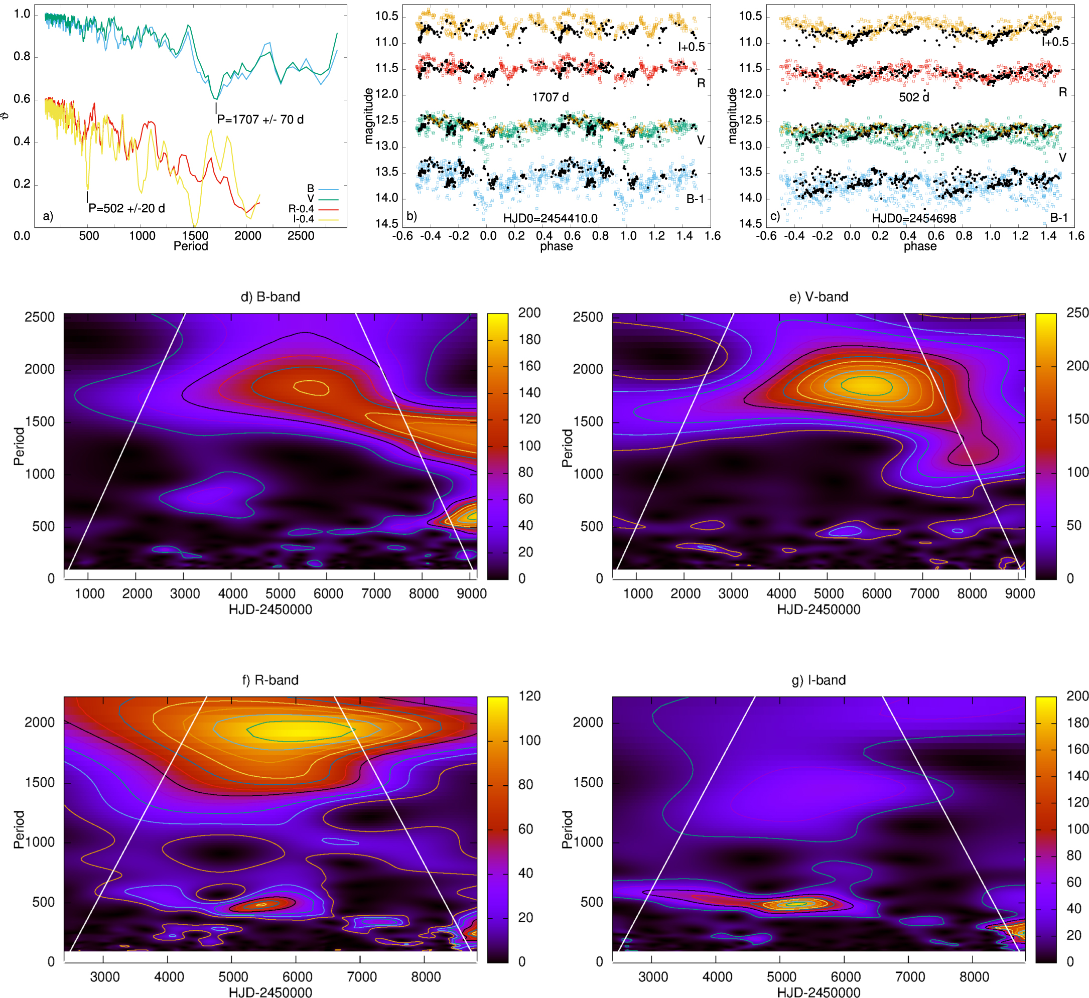
There remain several open questions related to the origin of variability in the photometric and spectroscopic data sets. Continuing long-term photometric observations, as well as snapshot spectroscopic observations at least once a year, will be essential to better understand the change in the accretion and outflow activity of V1057 Cyg. This study highlights the importance of expanding our knowledge on classical FUors, since studying them is crucial to identify new members of this class.
We kindly thank Michael Connelley for handing over to us the 2015 IRTF spectra of V1057 Cyg in order to carry out a more accurate analysis. Zs.M.Sz. is supported by the ÚNKP-20-2 New National Excellence Program of the Ministry for Innovation and Technology from the source of the National Research, Development and Innovation Fund. This project has received funding from the European Research Council (ERC) under the European Union's Horizon 2020 research and innovation program under grant agreement No. 716155 (SACCRED). The work was also supported by the Hungarian NKFIH grants K-132406, K-131508, and KH-130526 and by the NKFIH grant 2019-2.1.11-TÉT-2019-00056. Authors acknowledge the financial support of the Austrian-Hungarian Action Foundation (101öu13, 104öu2). L.K. acknowledges the financial support of the Hungarian National Research, Development and Innovation Office grant NKFIH PD-134784. Our study is supported by the project "Transient Astrophysical Objects" GINOP 2.3.2-15-2016-00033 of the National Research, Development and Innovation Office (NKFIH), Hungary, funded by the European Union. This project has been supported by the GINOP-2.3.2-15-2016-00003 grant of the Hungarian National Research, Development and Innovation Office (NKFIH). This project has been supported by the Lendület grant LP2012-31 of the Hungarian Academy of Sciences. J.-E.L. was supported by the Basic Science Research Program through the National Research Foundation of Korea (grant No. NRF-2018R1A2B6003423). This paper includes data collected by the TESS mission. Funding for the TESS mission is provided by the NASA Explorer Program. This project has been supported by the GINOP-2.3.2-15-2016-00003 grant of the Hungarian National Research, Development and Innovation Office (NKFIH). L.K. is supported by the Bolyai János Research Scholarship of the Hungarian Academy of Sciences. Based on observations made with the Nordic Optical Telescope, operated by the Nordic Optical Telescope Scientific Association at the Observatorio del Roque de los Muchachos, La Palma, Spain, of the Instituto de Astrofisica de Canarias. The data presented here were obtained (in part) with ALFOSC, which is provided by the Instituto de Astrofisica de Andalucia (IAA) under a joint agreement with the University of Copenhagen and NOTSA. Based (in part) on observations made with the NASA/DLR Stratospheric Observatory for Infrared Astronomy (SOFIA). SOFIA is jointly operated by the Universities Space Research Association, Inc. (USRA), under NASA contract NNA17BF53C, and the Deutsches SOFIA Institut (DSI) under DLR contract 50 OK 0901 to the University of Stuttgart.
Facilities: NOT - Nordic Optical Telescope, BOAO - , SOFIA - , TESS. -
Software: FITSH package (Pál 2012), Vartools (Hartman & Bakos 2016), molecfit (Kausch et al. 2015; Smette et al. 2015), IRAF (Tody 1986, 1993).
Appendix A: Photometry of V1057 Cyg
Table 4 contains our original optical and NIR photometry of V1057 Cyg before the shifts discussed in Section 2, while Table 5 contains the saturation-corrected WISE data that we use in Figure 1.
Table 4. Optical and NIR Photometry of V1057 Cyg
| Date | MJD | B | V | g' | RC | IC | RJ | IJ | r' | i' | J | H | Ks | Instrument |
|---|---|---|---|---|---|---|---|---|---|---|---|---|---|---|
| 2005-10-29 | 53672.75 | 14.43 | 12.53 | ⋯ | 11.52 | 10.54 | ⋯ | ⋯ | ⋯ | ⋯ | ⋯ | ⋯ | ⋯ | RCC |
| 2005-10-31 | 53674.75 | 14.43 | 12.51 | ⋯ | 11.51 | 10.51 | ⋯ | ⋯ | ⋯ | ⋯ | ⋯ | ⋯ | ⋯ | RCC |
| 2005-11-17 | 53691.74 | 14.51 | 12.66 | ⋯ | 11.61 | 10.59 | ⋯ | ⋯ | ⋯ | ⋯ | ⋯ | ⋯ | ⋯ | RCC |
| 2005-11-18 | 53692.82 | 14.26 | 12.61 | ⋯ | 11.60 | 10.50 | ⋯ | ⋯ | ⋯ | ⋯ | ⋯ | ⋯ | ⋯ | RCC |
| 2006-07-15 | 53932.12 | ⋯ | ⋯ | ⋯ | ⋯ | ⋯ | ⋯ | ⋯ | ⋯ | ⋯ | 8.08 | 7.27 | 6.25 | TCS |
| 2006-07-20 | 53936.92 | 14.53 | 12.51 | ⋯ | ⋯ | ⋯ | 11.39 | 10.42 | ⋯ | ⋯ | ⋯ | ⋯ | ⋯ | IAC80 |
| 2007-06-02 | 54254.22 | ⋯ | ⋯ | ⋯ | ⋯ | ⋯ | ⋯ | ⋯ | ⋯ | ⋯ | 8.52 | 7.19 | 7.29 | TCS |
| 2007-07-23 | 54304.92 | 14.56 | 12.71 | ⋯ | 11.62 | 10.49 | ⋯ | ⋯ | ⋯ | ⋯ | ⋯ | ⋯ | ⋯ | RCC |
| 2007-10-28 | 54401.94 | ⋯ | ⋯ | ⋯ | ⋯ | ⋯ ⋯ | ⋯ | ⋯ | ⋯ | ⋯ | 8.03 | ⋯ | 6.13 | TCS |
| 2011-03-23 | 55644.12 | 14.31 | 12.52 | ⋯ | 11.50 | 10.52 | ⋯ | ⋯ | ⋯ | ⋯ | ⋯ | ⋯ | ⋯ | Schmidt |
| 2011-04-10 | 55661.05 | 14.31 | 12.52 | ⋯ | 11.46 | 10.43 | ⋯ | ⋯ | ⋯ | ⋯ | ⋯ | ⋯ | ⋯ | Schmidt |
| 2011-06-19 | 55731.87 | 14.30 | 12.50 | ⋯ | 11.49 | 10.46 | ⋯ | ⋯ | ⋯ | ⋯ | ⋯ | ⋯ | ⋯ | Schmidt |
| 2011-06-20 | 55732.92 | 14.32 | 12.50 | ⋯ | 11.48 | ⋯ | ⋯ | ⋯ | ⋯ | ⋯ | ⋯ | ⋯ | ⋯ | Schmidt |
| 2011-08-05 | 55778.95 | 14.14 | 12.42 | ⋯ | ⋯ | ⋯ | ⋯ | ⋯ | ⋯ | ⋯ | ⋯ | ⋯ | ⋯ | Schmidt |
| 2011-08-11 | 55784.88 | 14.14 | 12.40 | ⋯ | ⋯ | ⋯ | ⋯ | ⋯ | ⋯ | ⋯ | ⋯ | ⋯ | ⋯ | Schmidt |
| 2011-08-12 | 55785.86 | 14.11 | ⋯ | ⋯ | ⋯ | ⋯ | ⋯ | ⋯ | ⋯ | ⋯ | ⋯ | ⋯ | ⋯ | Schmidt |
| 2011-08-14 | 55787.83 | 14.18 | ⋯ | ⋯ | ⋯ | ⋯ | ⋯ | ⋯ | ⋯ | ⋯ | ⋯ | ⋯ | ⋯ | Schmidt |
| 2011-08-15 | 55788.81 | 14.21 | 12.42 | ⋯ | ⋯ | ⋯ ⋯ | ⋯ | ⋯ | ⋯ | ⋯ | ⋯ | ⋯ | ⋯ | Schmidt |
| 2011-08-15 | 55788.97 | ⋯ | ⋯ | ⋯ | ⋯ | ⋯ ⋯ | ⋯ | ⋯ | ⋯ | ⋯ | 8.13 | 7.31 | 6.40 | TCS |
| 2011-08-17 | 55790.91 | 14.14 | 12.41 | ⋯ | ⋯ | ⋯ | ⋯ | ⋯ | ⋯ | ⋯ | ⋯ | ⋯ | ⋯ | Schmidt |
| 2011-08-18 | 55792.05 | 14.19 | 12.44 | ⋯ | ⋯ | ⋯ | ⋯ | ⋯ | ⋯ | ⋯ | ⋯ | ⋯ | ⋯ | Schmidt |
| 2011-08-20 | 55793.98 | 14.19 | 12.45 | ⋯ | ⋯ | ⋯ | ⋯ | ⋯ | ⋯ | ⋯ | ⋯ | ⋯ | ⋯ | Schmidt |
| 2011-08-23 | 55797.06 | 14.16 | 12.41 | ⋯ | ⋯ | ⋯ | ⋯ | ⋯ | ⋯ | ⋯ | ⋯ | ⋯ | ⋯ | Schmidt |
| 2011-09-02 | 55807.01 | 14.18 | 12.43 | ⋯ | ⋯ | ⋯ | ⋯ | ⋯ | ⋯ | ⋯ | ⋯ | ⋯ | ⋯ | Schmidt |
| 2011-09-06 | 55810.80 | 14.25 | 12.43 | ⋯ | 11.42 | ⋯ | ⋯ | ⋯ | ⋯ | ⋯ | ⋯ | ⋯ | ⋯ | Schmidt |
| 2011-09-09 | 55813.85 | 14.29 | 12.46 | ⋯ | 11.42 | ⋯ | ⋯ | ⋯ | ⋯ | ⋯ | ⋯ | ⋯ | ⋯ | Schmidt |
| 2011-09-12 | 55817.02 | ⋯ | ⋯ | ⋯ | ⋯ | ⋯ ⋯ | ⋯ | ⋯ | ⋯ | ⋯ | 8.25 | 7.26 | 6.37 | TCS |
| 2011-09-17 | 55821.82 | 14.24 | 12.40 | ⋯ | 11.35 | 10.30 | ⋯ | ⋯ | ⋯ | ⋯ | ⋯ | ⋯ | ⋯ | Schmidt |
| 2011-09-21 | 55825.86 | 14.26 | 12.39 | ⋯ | 11.36 | ⋯ | ⋯ | ⋯ | ⋯ | ⋯ | ⋯ | ⋯ | ⋯ | Schmidt |
| 2011-09-25 | 55829.78 | 14.24 | 12.37 | ⋯ | ⋯ | ⋯ | ⋯ | ⋯ | ⋯ | ⋯ | ⋯ | ⋯ | ⋯ | Schmidt |
| 2011-10-26 | 55860.74 | 14.43 | 12.47 | ⋯ | 11.39 | ⋯ | ⋯ | ⋯ | ⋯ | ⋯ | ⋯ | ⋯ | ⋯ | Schmidt |
| 2011-10-27 | 55861.78 | 14.39 | 12.47 | ⋯ | 11.40 | 10.25 | ⋯ | ⋯ | ⋯ | ⋯ | ⋯ | ⋯ | ⋯ | Schmidt |
| 2011-10-28 | 55862.70 | 14.39 | 12.47 | ⋯ | 11.40 | 10.25 | ⋯ | ⋯ | ⋯ | ⋯ | ⋯ | ⋯ | ⋯ | Schmidt |
| 2011-10-29 | 55863.92 | 14.35 | 12.51 | ⋯ | ⋯ | ⋯ | ⋯ | ⋯ | ⋯ | ⋯ | ⋯ | ⋯ | ⋯ | Schmidt |
| 2011-10-30 | 55864.90 | 14.29 | 12.46 | ⋯ | ⋯ | ⋯ | ⋯ | ⋯ | ⋯ | ⋯ | ⋯ | ⋯ | ⋯ | Schmidt |
| 2011-10-31 | 55865.89 | 14.32 | 12.49 | ⋯ | ⋯ | ⋯ | ⋯ | ⋯ | ⋯ | ⋯ | ⋯ | ⋯ | ⋯ | Schmidt |
| 2011-11-01 | 55866.73 | 14.37 | 12.52 | ⋯ | ⋯ | ⋯ | ⋯ | ⋯ | ⋯ | ⋯ | ⋯ | ⋯ | ⋯ | Schmidt |
| 2011-11-02 | 55867.72 | 14.35 | 12.53 | ⋯ | ⋯ | ⋯ | ⋯ | ⋯ | ⋯ | ⋯ | ⋯ | ⋯ | ⋯ | Schmidt |
| 2011-11-03 | 55868.88 | 14.37 | 12.48 | ⋯ | 11.41 | 10.28 | ⋯ | ⋯ | ⋯ | ⋯ | ⋯ | ⋯ | ⋯ | Schmidt |
| 2011-11-22 | 55887.68 | 14.36 | 12.48 | ⋯ | 11.36 | ⋯ | ⋯ | ⋯ | ⋯ | ⋯ | ⋯ | ⋯ | ⋯ | Schmidt |
| 2011-11-23 | 55888.68 | 14.35 | 12.53 | ⋯ | ⋯ | ⋯ | ⋯ | ⋯ | ⋯ | ⋯ | ⋯ | ⋯ | ⋯ | Schmidt |
| 2011-11-24 | 55889.68 | 14.32 | 12.49 | ⋯ | ⋯ | ⋯ | ⋯ | ⋯ | ⋯ | ⋯ | ⋯ | ⋯ | ⋯ | Schmidt |
| 2011-11-25 | 55890.72 | 14.28 | 12.46 | ⋯ | ⋯ | ⋯ | ⋯ | ⋯ | ⋯ | ⋯ | ⋯ | ⋯ | ⋯ | Schmidt |
| 2011-11-27 | 55892.78 | 14.26 | 12.41 | ⋯ | ⋯ | ⋯ | ⋯ | ⋯ | ⋯ | ⋯ | ⋯ | ⋯ | ⋯ | Schmidt |
| 2011-11-27 | 55893.67 | 14.29 | 12.46 | ⋯ | ⋯ | ⋯ | ⋯ | ⋯ | ⋯ | ⋯ | ⋯ | ⋯ | ⋯ | Schmidt |
| 2011-11-28 | 55894.68 | 14.29 | 12.45 | ⋯ | 11.33 | 10.20 | ⋯ | ⋯ | ⋯ | ⋯ | ⋯ | ⋯ | ⋯ | Schmidt |
| 2011-11-29 | 55895.73 | 14.30 | 12.44 | ⋯ | 11.46 | 10.31 | ⋯ | ⋯ | ⋯ | ⋯ | ⋯ | ⋯ | ⋯ | Schmidt |
| 2011-12-31 | 55926.67 | 14.36 | 12.48 | ⋯ | ⋯ | ⋯ | ⋯ | ⋯ | ⋯ | ⋯ | ⋯ | ⋯ | ⋯ | Schmidt |
| 2012-02-10 | 55967.71 | 14.99 | 12.97 | ⋯ | 11.81 | 10.57 | ⋯ | ⋯ | ⋯ | ⋯ | ⋯ | ⋯ | ⋯ | Schmidt |
| 2012-04-27 | 56045.09 | 14.51 | 12.65 | ⋯ | 11.57 | 10.52 | ⋯ | ⋯ | ⋯ | ⋯ | ⋯ | ⋯ | ⋯ | Schmidt |
| 2012-05-31 | 56079.02 | 14.28 | 12.47 | ⋯ | 11.47 | 10.42 | ⋯ | ⋯ | ⋯ | ⋯ | ⋯ | ⋯ | ⋯ | Schmidt |
| 2012-06-07 | 56085.95 | 14.24 | 12.52 | ⋯ | 11.43 | 10.41 | ⋯ | ⋯ | ⋯ | ⋯ | ⋯ | ⋯ | ⋯ | Schmidt |
| 2012-06-19 | 56097.99 | 14.29 | 12.52 | ⋯ | 11.49 | 10.46 | ⋯ | ⋯ | ⋯ | ⋯ | ⋯ | ⋯ | ⋯ | Schmidt |
| 2012-07-22 | 56130.82 | 14.41 | 12.57 | ⋯ | 11.57 | 10.63 | ⋯ | ⋯ | ⋯ | ⋯ | ⋯ | ⋯ | ⋯ | Schmidt |
| 2012-07-23 | 56131.82 | 14.39 | 12.57 | ⋯ | 11.59 | ⋯ | ⋯ | ⋯ | ⋯ | ⋯ | ⋯ | ⋯ | ⋯ | Schmidt |
| 2012-10-13 | 56214.05 | ⋯ | ⋯ | ⋯ | ⋯ | ⋯ ⋯ | ⋯ | ⋯ | ⋯ | ⋯ | 8.23 | 7.22 | 6.41 | TCS |
| 2012-10-14 | 56214.01 | ⋯ | 12.58 | ⋯ | ⋯ | ⋯ | 11.58 | 10.59 | ⋯ | ⋯ | ⋯ | ⋯ | ⋯ | IAC80 |
| 2013-07-23 | 56497.04 | ⋯ | 12.62 | ⋯ | ⋯ | ⋯ | ⋯ | ⋯ | ⋯ | ⋯ | ⋯ | ⋯ | ⋯ | Schmidt |
| 2013-08-08 | 56512.86 | 14.62 | 12.72 | ⋯ | ⋯ | 10.65 | ⋯ | ⋯ | ⋯ | ⋯ | ⋯ | ⋯ | ⋯ | Schmidt |
| 2013-08-17 | 56521.91 | 14.75 | 12.81 | ⋯ | ⋯ | 10.6 | ⋯ | ⋯ | ⋯ | ⋯ | ⋯ | ⋯ | ⋯ | Schmidt |
| 2014-02-23 | 56712.16 | 14.31 | 12.41 | ⋯ | 11.35 | 10.25 | ⋯ | ⋯ | ⋯ | ⋯ | ⋯ | ⋯ | ⋯ | Schmidt |
| 2014-04-07 | 56755.10 | 14.32 | 12.41 | ⋯ | 11.36 | 10.28 | ⋯ | ⋯ | ⋯ | ⋯ | ⋯ | ⋯ | ⋯ | Schmidt |
| 2014-04-29 | 56777.08 | 14.30 | 12.37 | ⋯ | 11.31 | ⋯ | ⋯ | ⋯ | ⋯ | ⋯ | ⋯ | ⋯ | ⋯ | Schmidt |
| 2014-06-04 | 56813.03 | 14.31 | 12.40 | ⋯ | 11.34 | ⋯ | ⋯ | ⋯ | ⋯ | ⋯ | ⋯ | ⋯ | ⋯ | Schmidt |
| 2014-06-06 | 57028.71 | 14.15 | 12.30 | ⋯ | 11.27 | 10.24 | ⋯ | ⋯ | ⋯ | ⋯ | ⋯ | ⋯ | ⋯ | Schmidt |
| 2015-02-16 | 57070.18 | 14.14 | 12.31 | ⋯ | 11.32 | 10.29 | ⋯ | ⋯ | ⋯ | ⋯ | ⋯ | ⋯ | ⋯ | Schmidt |
| 2015-02-17 | 57071.17 | 14.13 | 12.36 | ⋯ | 11.36 | 10.34 | ⋯ | ⋯ | ⋯ | ⋯ | ⋯ | ⋯ | ⋯ | Schmidt |
| 2015-03-16 | 57098.13 | 14.14 | 12.34 | ⋯ | 11.33 | 10.35 | ⋯ | ⋯ | ⋯ | ⋯ | ⋯ | ⋯ | ⋯ | Schmidt |
| 2015-04-08 | 57121.11 | 14.20 | 12.39 | ⋯ | 11.38 | 10.38 | ⋯ | ⋯ | ⋯ | ⋯ | ⋯ | ⋯ | ⋯ | Schmidt |
| 2015-04-12 | 57125.09 | 14.10 | 12.33 | ⋯ | 11.35 | 10.34 | ⋯ | ⋯ | ⋯ | ⋯ | ⋯ | ⋯ | ⋯ | Schmidt |
| 2015-04-19 | 57132.02 | 14.11 | 12.33 | ⋯ | 11.35 | 10.34 | ⋯ | ⋯ | ⋯ | ⋯ | ⋯ | ⋯ | ⋯ | Schmidt |
| 2015-04-22 | 57135.06 | 14.07 | 12.30 | ⋯ | 11.34 | 10.32 | ⋯ | ⋯ | ⋯ | ⋯ | ⋯ | ⋯ | ⋯ | Schmidt |
| 2015-05-07 | 57150.01 | 14.16 | 12.36 | ⋯ | 11.27 | 10.36 | ⋯ | ⋯ | ⋯ | ⋯ | ⋯ | ⋯ | ⋯ | Schmidt |
| 2015-05-16 | 57158.93 | 14.17 | 12.38 | ⋯ | 11.37 | 10.37 | ⋯ | ⋯ | ⋯ | ⋯ | ⋯ | ⋯ | ⋯ | Schmidt |
| 2015-05-31 | 57174.04 | 14.24 | 12.45 | ⋯ | ⋯ | ⋯ | ⋯ | ⋯ | ⋯ | ⋯ | ⋯ | ⋯ | ⋯ | Schmidt |
| 2015-06-03 | 57176.94 | 14.25 | 12.41 | ⋯ | 11.42 | 10.41 | ⋯ | ⋯ | ⋯ | ⋯ | ⋯ | ⋯ | ⋯ | Schmidt |
| 2015-06-06 | 57179.98 | 14.21 | 12.42 | ⋯ | 11.50 | 10.55 | ⋯ | ⋯ | ⋯ | ⋯ | ⋯ | ⋯ | ⋯ | Schmidt |
| 2015-06-07 | 57180.98 | 14.21 | 12.39 | ⋯ | 11.42 | 10.40 | ⋯ | ⋯ | ⋯ | ⋯ | ⋯ | ⋯ | ⋯ | Schmidt |
| 2015-06-12 | 57185.95 | 14.21 | 12.42 | ⋯ | 11.45 | 10.45 | ⋯ | ⋯ | ⋯ | ⋯ | ⋯ | ⋯ | ⋯ | Schmidt |
| 2015-06-17 | 57191.01 | 14.20 | 12.41 | ⋯ | 11.42 | 10.42 | ⋯ | ⋯ | ⋯ | ⋯ | ⋯ | ⋯ | ⋯ | Schmidt |
| 2015-07-16 | 57219.99 | 14.16 | 12.38 | ⋯ | 11.48 | 10.52 | ⋯ | ⋯ | ⋯ | ⋯ | ⋯ | ⋯ | ⋯ | Schmidt |
| 2015-07-22 | 57225.93 | 14.22 | 12.44 | ⋯ | 11.45 | 10.47 | ⋯ | ⋯ | ⋯ | ⋯ | ⋯ | ⋯ | ⋯ | Schmidt |
| 2015-08-05 | 57239.85 | 14.27 | 12.47 | ⋯ | ⋯ | ⋯ | ⋯ | ⋯ | ⋯ | ⋯ | ⋯ | ⋯ | ⋯ | Schmidt |
| 2015-08-12 | 57246.82 | 14.35 | 12.52 | ⋯ | 11.49 | 10.51 | ⋯ | ⋯ | ⋯ | ⋯ | ⋯ | ⋯ | ⋯ | Schmidt |
| 2015-08-31 | 57265.87 | 14.27 | 12.44 | ⋯ | 11.51 | 10.54 | ⋯ | ⋯ | ⋯ | ⋯ | ⋯ | ⋯ | ⋯ | Schmidt |
| 2015-09-01 | 57266.83 | 14.27 | 12.44 | ⋯ | 11.46 | 10.43 | ⋯ | ⋯ | ⋯ | ⋯ | ⋯ | ⋯ | ⋯ | Schmidt |
| 2015-09-02 | 57267.82 | 14.28 | 12.43 | ⋯ | 11.45 | 10.43 | ⋯ | ⋯ | ⋯ | ⋯ | ⋯ | ⋯ | ⋯ | Schmidt |
| 2015-09-15 | 57280.83 | 14.27 | 12.38 | ⋯ | 11.35 | 10.35 | ⋯ | ⋯ | ⋯ | ⋯ | ⋯ | ⋯ | ⋯ | Schmidt |
| 2015-09-17 | 57282.75 | 14.35 | 12.38 | ⋯ | ⋯ | ⋯ | ⋯ | ⋯ | ⋯ | ⋯ | ⋯ | ⋯ | ⋯ | Schmidt |
| 2015-09-18 | 57283.75 | 14.35 | 12.39 | ⋯ | 11.37 | 10.33 | ⋯ | ⋯ | ⋯ | ⋯ | ⋯ | ⋯ | ⋯ | Schmidt |
| 2015-10-22 | 57317.75 | 14.64 | 12.33 | ⋯ | 11.29 | ⋯ | ⋯ | ⋯ | ⋯ | ⋯ | ⋯ | ⋯ | ⋯ | Schmidt |
| 2015-10-27 | 57322.82 | ⋯ | 12.34 | ⋯ | 11.29 | ⋯ | ⋯ | ⋯ | ⋯ | ⋯ | ⋯ | ⋯ | ⋯ | Schmidt |
| 2015-11-05 | 57331.69 | ⋯ | 12.31 | ⋯ | 11.26 | 10.20 | ⋯ | ⋯ | ⋯ | ⋯ | ⋯ | ⋯ | ⋯ | Schmidt |
| 2015-11-08 | 57334.69 | ⋯ | 12.33 | ⋯ | 11.30 | 10.21 | ⋯ | ⋯ | ⋯ | ⋯ | ⋯ | ⋯ | ⋯ | Schmidt |
| 2015-11-12 | 57338.80 | ⋯ | ⋯ | ⋯ | 11.26 | 10.19 | ⋯ | ⋯ | ⋯ | ⋯ | ⋯ | ⋯ | ⋯ | Schmidt |
| 2015-12-26 | 57382.69 | 14.29 | 12.41 | ⋯ | 11.33 | 10.25 | ⋯ | ⋯ | ⋯ | ⋯ | ⋯ | ⋯ | ⋯ | Schmidt |
| 2016-04-29 | 57508.05 | 14.37 | 12.44 | ⋯ | 11.33 | ⋯ | ⋯ | ⋯ | ⋯ | ⋯ | ⋯ | ⋯ | ⋯ | Schmidt |
| 2016-05-06 | 57515.03 | 14.36 | 12.45 | ⋯ | 11.37 | 10.25 | ⋯ | ⋯ | ⋯ | ⋯ | ⋯ | ⋯ | ⋯ | Schmidt |
| 2016-05-21 | 57529.94 | 14.42 | 12.52 | ⋯ | ⋯ | ⋯ | ⋯ | ⋯ | ⋯ | ⋯ | ⋯ | ⋯ | ⋯ | Schmidt |
| 2016-05-29 | 57537.98 | 14.41 | 12.51 | ⋯ | 11.42 | 10.35 | ⋯ | ⋯ | ⋯ | ⋯ | ⋯ | ⋯ | ⋯ | Schmidt |
| 2016-05-30 | 57539.03 | 14.46 | 12.55 | ⋯ | 11.52 | 10.52 | ⋯ | ⋯ | ⋯ | ⋯ | ⋯ | ⋯ | ⋯ | Schmidt |
| 2016-06-08 | 57547.96 | 14.37 | 12.55 | ⋯ | 11.47 | 10.39 | ⋯ | ⋯ | ⋯ | ⋯ | ⋯ | ⋯ | ⋯ | Schmidt |
| 2016-06-23 | 57562.92 | 14.46 | 12.54 | ⋯ | 11.49 | 10.35 | ⋯ | ⋯ | ⋯ | ⋯ | ⋯ | ⋯ | ⋯ | Schmidt |
| 2016-07-06 | 57575.94 | 14.33 | 12.50 | ⋯ | 11.47 | 10.45 | ⋯ | ⋯ | ⋯ | ⋯ | ⋯ | ⋯ | ⋯ | Schmidt |
| 2016-07-11 | 57581.03 | 14.38 | 12.54 | ⋯ | 11.50 | 10.47 | ⋯ | ⋯ | ⋯ | ⋯ | ⋯ | ⋯ | ⋯ | Schmidt |
| 2016-07-12 | 57581.97 | 14.37 | 12.53 | ⋯ | 11.48 | 10.48 | ⋯ | ⋯ | ⋯ | ⋯ | ⋯ | ⋯ | ⋯ | Schmidt |
| 2016-08-04 | 57604.84 | 14.42 | 12.57 | ⋯ | 11.51 | ⋯ | ⋯ | ⋯ | ⋯ | ⋯ | ⋯ | ⋯ | ⋯ | Schmidt |
| 2016-08-14 | 57614.87 | 14.43 | 12.57 | ⋯ | 11.48 | 10.46 | ⋯ | ⋯ | ⋯ | ⋯ | ⋯ | ⋯ | ⋯ | Schmidt |
| 2016-09-01 | 57632.88 | 14.34 | 12.44 | ⋯ | 11.39 | 10.34 | ⋯ | ⋯ | ⋯ | ⋯ | ⋯ | ⋯ | ⋯ | Schmidt |
| 2016-09-13 | 57644.81 | 14.38 | 12.45 | ⋯ | 11.40 | 10.33 | ⋯ | ⋯ | ⋯ | ⋯ | ⋯ | ⋯ | ⋯ | Schmidt |
| 2016-09-22 | 57653.79 | 14.39 | 12.47 | ⋯ | 11.41 | 10.32 | ⋯ | ⋯ | ⋯ | ⋯ | ⋯ | ⋯ | ⋯ | Schmidt |
| 2017-04-09 | 57853.09 | 14.50 | 12.59 | ⋯ | 11.50 | 10.38 | ⋯ | ⋯ | ⋯ | ⋯ | ⋯ | ⋯ | ⋯ | Schmidt |
| 2017-04-14 | 57858.06 | 14.57 | 12.62 | ⋯ | 11.54 | 10.41 | ⋯ | ⋯ | ⋯ | ⋯ | ⋯ | ⋯ | ⋯ | Schmidt |
| 2017-04-16 | 57860.10 | 14.59 | 12.64 | ⋯ | 11.55 | 10.42 | ⋯ | ⋯ | ⋯ | ⋯ | ⋯ | ⋯ | ⋯ | Schmidt |
| 2017-04-30 | 57874.04 | 14.61 | 12.68 | ⋯ | 11.57 | 10.42 | ⋯ | ⋯ | ⋯ | ⋯ | ⋯ | ⋯ | ⋯ | Schmidt |
| 2017-05-02 | 57876.06 | 14.66 | 12.71 | ⋯ | 11.57 | 10.43 | ⋯ | ⋯ | ⋯ | ⋯ | ⋯ | ⋯ | ⋯ | Schmidt |
| 2017-05-10 | 57883.98 | 14.56 | 12.62 | ⋯ | 11.51 | 10.40 | ⋯ | ⋯ | ⋯ | ⋯ | ⋯ | ⋯ | ⋯ | Schmidt |
| 2017-05-18 | 57892.03 | 14.52 | 12.60 | ⋯ | 11.49 | ⋯ | ⋯ | ⋯ | ⋯ | ⋯ | ⋯ | ⋯ | ⋯ | Schmidt |
| 2017-05-19 | 57893.01 | 14.50 | 12.59 | ⋯ | 11.50 | 10.38 | ⋯ | ⋯ | ⋯ | ⋯ | ⋯ | ⋯ | ⋯ | Schmidt |
| 2017-05-21 | 57894.98 | 14.50 | 12.59 | ⋯ | 11.49 | 10.37 | ⋯ | ⋯ | ⋯ | ⋯ | ⋯ | ⋯ | ⋯ | Schmidt |
| 2017-05-25 | 57898.99 | 14.59 | 12.65 | ⋯ | 11.55 | 10.41 | ⋯ | ⋯ | ⋯ | ⋯ | ⋯ | ⋯ | ⋯ | Schmidt |
| 2017-05-28 | 57902.03 | 14.65 | 12.71 | ⋯ | 11.57 | 10.45 | ⋯ | ⋯ | ⋯ | ⋯ | ⋯ | ⋯ | ⋯ | Schmidt |
| 2017-06-01 | 57905.97 | 14.60 | 12.69 | ⋯ | 11.57 | 10.40 | ⋯ | ⋯ | ⋯ | ⋯ | ⋯ | ⋯ | ⋯ | Schmidt |
| 2017-06-03 | 57907.97 | 14.68 | 12.69 | ⋯ | 11.59 | 10.45 | ⋯ | ⋯ | ⋯ | ⋯ | ⋯ | ⋯ | ⋯ | Schmidt |
| 2017-06-08 | 57912.94 | 14.58 | 12.65 | ⋯ | 11.56 | 10.41 | ⋯ | ⋯ | ⋯ | ⋯ | ⋯ | ⋯ | ⋯ | Schmidt |
| 2017-06-09 | 57913.96 | 14.57 | 12.65 | ⋯ | 11.55 | 10.42 | ⋯ | ⋯ | ⋯ | ⋯ | ⋯ | ⋯ | ⋯ | Schmidt |
| 2017-06-10 | 57914.98 | 14.54 | 12.62 | ⋯ | 11.53 | 10.39 | ⋯ | ⋯ | ⋯ | ⋯ | ⋯ | ⋯ | ⋯ | Schmidt |
| 2017-06-11 | 57915.96 | 14.53 | 12.60 | ⋯ | 11.51 | 10.37 | ⋯ | ⋯ | ⋯ | ⋯ | ⋯ | ⋯ | ⋯ | Schmidt |
| 2017-06-15 | 57920.01 | 14.49 | 12.58 | ⋯ | 11.48 | 10.37 | ⋯ | ⋯ | ⋯ | ⋯ | ⋯ | ⋯ | ⋯ | Schmidt |
| 2017-06-19 | 57923.98 | 14.51 | 12.59 | ⋯ | 11.48 | 10.40 | ⋯ | ⋯ | ⋯ | ⋯ | ⋯ | ⋯ | ⋯ | Schmidt |
| 2017-06-21 | 57925.96 | 14.50 | 12.58 | ⋯ | 11.49 | 10.36 | ⋯ | ⋯ | ⋯ | ⋯ | ⋯ | ⋯ | ⋯ | Schmidt |
| 2017-06-24 | 57929.03 | 14.53 | 12.56 | ⋯ | 11.45 | 10.35 | ⋯ | ⋯ | ⋯ | ⋯ | ⋯ | ⋯ | ⋯ | Schmidt |
| 2017-06-26 | 57931.02 | 14.49 | 12.57 | ⋯ | 11.46 | 10.35 | ⋯ | ⋯ | ⋯ | ⋯ | ⋯ | ⋯ | ⋯ | Schmidt |
| 2017-07-06 | 57940.92 | 14.45 | 12.51 | ⋯ | 11.44 | 10.30 | ⋯ | ⋯ | ⋯ | ⋯ | ⋯ | ⋯ | ⋯ | Schmidt |
| 2017-07-08 | 57942.98 | 14.44 | 12.53 | ⋯ | 11.45 | 10.31 | ⋯ | ⋯ | ⋯ | ⋯ | ⋯ | ⋯ | ⋯ | Schmidt |
| 2017-07-13 | 57947.98 | 14.45 | 12.53 | ⋯ | 11.45 | 10.30 | ⋯ | ⋯ | ⋯ | ⋯ | ⋯ | ⋯ | ⋯ | Schmidt |
| 2017-07-17 | 57951.98 | 14.47 | 12.55 | ⋯ | 11.45 | 10.34 | ⋯ | ⋯ | ⋯ | ⋯ | ⋯ | ⋯ | ⋯ | Schmidt |
| 2017-07-20 | 57954.06 | 14.49 | 12.53 | ⋯ | 11.45 | 10.31 | ⋯ | ⋯ | ⋯ | ⋯ | ⋯ | ⋯ | ⋯ | Schmidt |
| 2017-11-24 | 58081.71 | 14.65 | 12.80 | ⋯ | 11.74 | 10.67 | ⋯ | ⋯ | ⋯ | ⋯ | ⋯ | ⋯ | ⋯ | Schmidt |
| 2018-05-03 | 58242.02 | 14.43 | 12.50 | ⋯ | 11.40 | 10.34 | ⋯ | ⋯ | ⋯ | ⋯ | ⋯ | ⋯ | ⋯ | Schmidt |
| 2018-05-20 | 58259.05 | 14.42 | 12.52 | ⋯ | 11.44 | 10.36 | ⋯ | ⋯ | ⋯ | ⋯ | ⋯ | ⋯ | ⋯ | Schmidt |
| 2018-05-22 | 58260.05 | 14.40 | 12.52 | ⋯ | 11.45 | 10.37 | ⋯ | ⋯ | ⋯ | ⋯ | ⋯ | ⋯ | ⋯ | Schmidt |
| 2018-05-23 | 58261.96 | 14.46 | 12.56 | ⋯ | 11.49 | 10.41 | ⋯ | ⋯ | ⋯ | ⋯ | ⋯ | ⋯ | ⋯ | Schmidt |
| 2018-06-01 | 58270.04 | 14.43 | 12.54 | ⋯ | 11.45 | 10.38 | ⋯ | ⋯ | ⋯ | ⋯ | ⋯ | ⋯ | ⋯ | Schmidt |
| 2018-06-08 | 58277.04 | 14.44 | 12.54 | ⋯ | 11.45 | 10.37 | ⋯ | ⋯ | ⋯ | ⋯ | ⋯ | ⋯ | ⋯ | Schmidt |
| 2018-06-10 | 58279.04 | 14.41 | 12.53 | ⋯ | 11.45 | 10.35 | ⋯ | ⋯ | ⋯ | ⋯ | ⋯ | ⋯ | ⋯ | Schmidt |
| 2018-06-11 | 58280.96 | 14.41 | 12.52 | ⋯ | 11.45 | 10.34 | ⋯ | ⋯ | ⋯ | ⋯ | ⋯ | ⋯ | ⋯ | Schmidt |
| 2018-07-03 | 58302.01 | 14.48 | 12.56 | ⋯ | 11.47 | 10.34 | ⋯ | ⋯ | ⋯ | ⋯ | ⋯ | ⋯ | ⋯ | Schmidt |
| 2019-05-10 | 58613.99 | 14.45 | 12.55 | ⋯ | 11.47 | 10.43 | ⋯ | ⋯ | ⋯ | ⋯ | ⋯ | ⋯ | ⋯ | Schmidt |
| 2019-05-25 | 58628.99 | 14.37 | 12.49 | ⋯ | 11.45 | 10.43 | ⋯ | ⋯ | ⋯ | ⋯ | ⋯ | ⋯ | ⋯ | Schmidt |
| 2019-05-26 | 58629.97 | 14.38 | 12.50 | ⋯ | 11.45 | 10.44 | ⋯ | ⋯ | ⋯ | ⋯ | ⋯ | ⋯ | ⋯ | Schmidt |
| 2019-06-09 | 58643.98 | 14.32 | 12.49 | ⋯ | 11.47 | 10.47 | ⋯ | ⋯ | ⋯ | ⋯ | ⋯ | ⋯ | ⋯ | Schmidt |
| 2019-06-28 | 58663.03 | 14.40 | 12.56 | ⋯ | 11.53 | 10.53 | ⋯ | ⋯ | ⋯ | ⋯ | ⋯ | ⋯ | ⋯ | Schmidt |
| 2019-08-09 | 58704.91 | 14.42 | 12.60 | ⋯ | 11.60 | 10.58 | ⋯ | ⋯ | ⋯ | ⋯ | ⋯ | ⋯ | ⋯ | Schmidt |
| 2019-08-10 | 58705.94 | 14.37 | 12.57 | ⋯ | 11.57 | 10.56 | ⋯ | ⋯ | ⋯ | ⋯ | ⋯ | ⋯ | ⋯ | Schmidt |
| 2019-08-11 | 58706.91 | 14.39 | 12.57 | ⋯ | 11.56 | 10.53 | ⋯ | ⋯ | ⋯ | ⋯ | ⋯ | ⋯ | ⋯ | Schmidt |
| 2019-08-12 | 58707.91 | 14.37 | 12.57 | ⋯ | 11.56 | 10.53 | ⋯ | ⋯ | ⋯ | ⋯ | ⋯ | ⋯ | ⋯ | Schmidt |
| 2019-08-15 | 58710.92 | 14.38 | 12.59 | ⋯ | 11.53 | 10.62 | ⋯ | ⋯ | ⋯ | ⋯ | ⋯ | ⋯ | ⋯ | Schmidt |
| 2019-08-16 | 58711.96 | 14.39 | 12.56 | ⋯ | 11.54 | 10.53 | ⋯ | ⋯ | ⋯ | ⋯ | ⋯ | ⋯ | ⋯ | Schmidt |
| 2019-08-17 | 58712.99 | 14.39 | 12.59 | ⋯ | 11.54 | 10.56 | ⋯ | ⋯ | ⋯ | ⋯ | ⋯ | ⋯ | ⋯ | Schmidt |
| 2019-08-18 | 58713.93 | 14.39 | 12.57 | ⋯ | 11.54 | 10.54 | ⋯ | ⋯ | ⋯ | ⋯ | ⋯ | ⋯ | ⋯ | Schmidt |
| 2019-08-19 | 58714.94 | 14.37 | 12.58 | ⋯ | 11.55 | 10.56 | ⋯ | ⋯ | ⋯ | ⋯ | ⋯ | ⋯ | ⋯ | Schmidt |
| 2019-08-23 | 58718.86 | 14.33 | 12.55 | ⋯ | 11.55 | 10.54 | ⋯ | ⋯ | ⋯ | ⋯ | ⋯ | ⋯ | ⋯ | Schmidt |
| 2019-08-24 | 58719.79 | 14.41 | 12.58 | ⋯ | 11.53 | 10.58 | ⋯ | ⋯ | ⋯ | ⋯ | ⋯ | ⋯ | ⋯ | Schmidt |
| 2019-08-25 | 58720.79 | 14.38 | 12.56 | ⋯ | 11.53 | 10.54 | ⋯ | ⋯ | ⋯ | ⋯ | ⋯ | ⋯ | ⋯ | Schmidt |
| 2019-08-26 | 58721.80 | 14.38 | 12.58 | ⋯ | 11.54 | 10.55 | ⋯ | ⋯ | ⋯ | ⋯ | ⋯ | ⋯ | ⋯ | Schmidt |
| 2019-08-27 | 58722.79 | ⋯ | 12.58 | ⋯ | 11.62 | 10.61 | ⋯ | ⋯ | ⋯ | ⋯ | ⋯ | ⋯ | ⋯ | Schmidt |
| 2019-08-28 | 58723.81 | 14.38 | 12.57 | ⋯ | 11.54 | 10.53 | ⋯ | ⋯ | ⋯ | ⋯ | ⋯ | ⋯ | ⋯ | Schmidt |
| 2019-08-29 | 58724.97 | 14.43 | 12.57 | ⋯ | 11.54 | 10.56 | ⋯ | ⋯ | ⋯ | ⋯ | ⋯ | ⋯ | ⋯ | Schmidt |
| 2019-08-30 | 58725.95 | 14.41 | 12.58 | ⋯ | 11.57 | 10.54 | ⋯ | ⋯ | ⋯ | ⋯ | ⋯ | ⋯ | ⋯ | Schmidt |
| 2019-08-31 | 58726.92 | 14.36 | 12.55 | ⋯ | 11.53 | 10.52 | ⋯ | ⋯ | ⋯ | ⋯ | ⋯ | ⋯ | ⋯ | Schmidt |
| 2019-09-03 | 58730.08 | 14.35 | 12.56 | ⋯ | 11.53 | 10.52 | ⋯ | ⋯ | ⋯ | ⋯ | ⋯ | ⋯ | ⋯ | Schmidt |
| 2019-09-10 | 58736.92 | 14.35 | 12.51 | ⋯ | 11.47 | 10.45 | ⋯ | ⋯ | ⋯ | ⋯ | ⋯ | ⋯ | ⋯ | Schmidt |
| 2019-09-12 | 58738.88 | 14.33 | 12.49 | ⋯ | 11.46 | 10.42 | ⋯ | ⋯ | ⋯ | ⋯ | ⋯ | ⋯ | ⋯ | Schmidt |
| 2019-09-13 | 58739.93 | 14.33 | 12.49 | ⋯ | 11.46 | 10.42 | ⋯ | ⋯ | ⋯ | ⋯ | ⋯ | ⋯ | ⋯ | Schmidt |
| 2019-09-14 | 58740.89 | 14.29 | 12.47 | ⋯ | 11.43 | 10.40 | ⋯ | ⋯ | ⋯ | ⋯ | ⋯ | ⋯ | ⋯ | Schmidt |
| 2019-09-15 | 58741.87 | 14.30 | 12.47 | ⋯ | 11.44 | 10.39 | ⋯ | ⋯ | ⋯ | ⋯ | ⋯ | ⋯ | ⋯ | Schmidt |
| 2019-09-18 | 58744.93 | 14.35 | 12.49 | ⋯ | 11.44 | 10.39 | ⋯ | ⋯ | ⋯ | ⋯ | ⋯ | ⋯ | ⋯ | Schmidt |
| 2019-09-20 | 58748.00 | 14.32 | 12.49 | ⋯ | 11.43 | 10.39 | ⋯ | ⋯ | ⋯ | ⋯ | ⋯ | ⋯ | ⋯ | Schmidt |
| 2019-09-26 | 58752.90 | 14.33 | 12.49 | ⋯ | 11.43 | 10.38 | ⋯ | ⋯ | ⋯ | ⋯ | ⋯ | ⋯ | ⋯ | Schmidt |
| 2019-10-01 | 58757.87 | 14.37 | 12.53 | ⋯ | 11.47 | 10.41 | ⋯ | ⋯ | ⋯ | ⋯ | ⋯ | ⋯ | ⋯ | Schmidt |
| 2019-10-07 | 58763.81 | 14.33 | 12.47 | ⋯ | 11.44 | 10.38 | ⋯ | ⋯ | ⋯ | ⋯ | ⋯ | ⋯ | ⋯ | Schmidt |
| 2019-10-10 | 58766.96 | 14.34 | 12.49 | ⋯ | 11.45 | 10.39 | ⋯ | ⋯ | ⋯ | ⋯ | ⋯ | ⋯ | ⋯ | Schmidt |
| 2019-10-11 | 58767.82 | 14.36 | 12.48 | ⋯ | 11.43 | 10.37 | ⋯ | ⋯ | ⋯ | ⋯ | ⋯ | ⋯ | ⋯ | Schmidt |
| 2019-10-12 | 58768.82 | 14.34 | 12.47 | ⋯ | 11.43 | 10.37 | ⋯ | ⋯ | ⋯ | ⋯ | ⋯ | ⋯ | ⋯ | Schmidt |
| 2019-10-14 | 58769.92 | 14.36 | 12.50 | ⋯ | 11.45 | 10.39 | ⋯ | ⋯ | ⋯ | ⋯ | ⋯ | ⋯ | ⋯ | Schmidt |
| 2019-10-15 | 58771.74 | 14.33 | 12.47 | ⋯ | 11.42 | 10.37 | ⋯ | ⋯ | ⋯ | ⋯ | ⋯ | ⋯ | ⋯ | Schmidt |
| 2019-10-20 | 58776.87 | 14.37 | 12.53 | ⋯ | 11.47 | 10.38 | ⋯ | ⋯ | ⋯ | ⋯ | ⋯ | ⋯ | ⋯ | Schmidt |
| 2019-10-22 | 58778.79 | 14.36 | 12.51 | ⋯ | 11.45 | 10.38 | ⋯ | ⋯ | ⋯ | ⋯ | ⋯ | ⋯ | ⋯ | Schmidt |
| 2019-10-24 | 58780.85 | 14.36 | 12.48 | ⋯ | 11.43 | 10.35 | ⋯ | ⋯ | ⋯ | ⋯ | ⋯ | ⋯ | ⋯ | Schmidt |
| 2019-10-25 | 58781.83 | 14.33 | 12.47 | ⋯ | 11.42 | 10.35 | ⋯ | ⋯ | ⋯ | ⋯ | ⋯ | ⋯ | ⋯ | Schmidt |
| 2019-12-01 | 58818.71 | 14.24 | 12.46 | ⋯ | 11.38 | 10.32 | ⋯ | ⋯ | ⋯ | ⋯ | ⋯ | ⋯ | ⋯ | Schmidt |
| 2019-12-04 | 58821.75 | 14.32 | 12.45 | ⋯ | 11.34 | 10.31 | ⋯ | ⋯ | ⋯ | ⋯ | ⋯ | ⋯ | ⋯ | Schmidt |
| 2020-07-12 | 59043.06 | 14.62 | 12.69 | ⋯ | ⋯ | ⋯ | ⋯ | ⋯ | 11.89 | 11.09 | ⋯ | ⋯ | ⋯ | RC80 |
| 2020-07-14 | 59045.06 | 14.59 | 12.68 | ⋯ | ⋯ | ⋯ | ⋯ | ⋯ | 11.87 | 11.08 | ⋯ | ⋯ | ⋯ | RC80 |
| 2020-07-15 | 59045.88 | 14.64 | 12.69 | ⋯ | ⋯ | ⋯ | ⋯ | ⋯ | 11.89 | 11.10 | ⋯ | ⋯ | ⋯ | RC80 |
| 2020-07-21 | 59052.06 | 14.56 | 12.62 | ⋯ | ⋯ | ⋯ | ⋯ | ⋯ | 11.84 | 7.34 | ⋯ | ⋯ | ⋯ | RC80 |
| 2020-07-23 | 59054.05 | 14.53 | 12.59 | ⋯ | ⋯ | ⋯ | ⋯ | ⋯ | 11.81 | 11.00 | ⋯ | ⋯ | ⋯ | RC80 |
| 2020-07-27 | 59058.05 | 14.48 | 12.56 | ⋯ | ⋯ | ⋯ | ⋯ | ⋯ | 11.78 | 10.96 | ⋯ | ⋯ | ⋯ | RC80 |
| 2020-07-30 | 59060.90 | 14.50 | 12.57 | ⋯ | ⋯ | ⋯ | ⋯ | ⋯ | 11.78 | 10.97 | ⋯ | ⋯ | ⋯ | RC80 |
| 2020-07-31 | 59061.84 | 14.51 | 12.60 | ⋯ | ⋯ | ⋯ | ⋯ | ⋯ | 11.81 | 10.99 | ⋯ | ⋯ | ⋯ | RC80 |
| 2020-08-01 | 59062.83 | 14.54 | 12.60 | ⋯ | ⋯ | ⋯ | ⋯ | ⋯ | 11.82 | 11.01 | ⋯ | ⋯ | ⋯ | RC80 |
| 2020-08-06 | 59067.83 | 14.53 | 12.63 | ⋯ | ⋯ | ⋯ | ⋯ | ⋯ | 11.83 | 11.00 | ⋯ | ⋯ | ⋯ | RC80 |
| 2020-08-07 | 59068.83 | 14.57 | 12.63 | ⋯ | ⋯ | ⋯ | ⋯ | ⋯ | 11.83 | 11.00 | ⋯ | ⋯ | ⋯ | RC80 |
| 2020-08-08 | 59069.83 | 14.58 | 12.63 | ⋯ | ⋯ | ⋯ | ⋯ | ⋯ | 11.83 | 11.01 | ⋯ | ⋯ | ⋯ | RC80 |
| 2020-08-09 | 59070.82 | 14.58 | 12.62 | ⋯ | ⋯ | ⋯ | ⋯ | ⋯ | 11.83 | 11.00 | ⋯ | ⋯ | ⋯ | RC80 |
| 2020-08-11 | 59072.84 | 14.61 | 12.66 | ⋯ | ⋯ | ⋯ | ⋯ | ⋯ | 11.82 | 11.01 | ⋯ | ⋯ | ⋯ | RC80 |
| 2020-08-12 | 59073.98 | 14.56 | 12.60 | ⋯ | ⋯ | ⋯ | ⋯ | ⋯ | 11.80 | 10.96 | ⋯ | ⋯ | ⋯ | RC80 |
| 2020-08-13 | 59074.42 | 14.57 | 12.61 | ⋯ | ⋯ | ⋯ | ⋯ | ⋯ | 11.81 | 10.97 | ⋯ | ⋯ | ⋯ | RC80 |
| 2020-08-14 | 59074.42 | 14.60 | 12.63 | ⋯ | ⋯ | ⋯ | ⋯ | ⋯ | 11.84 | 11.00 | ⋯ | ⋯ | ⋯ | RC80 |
| 2020-08-17 | 59078.52 | 14.53 | 12.72 | ⋯ | 11.53 | ⋯ | ⋯ | ⋯ | ⋯ | 10.75 | ⋯ | ⋯ | ⋯ | NOT |
| 2020-08-20 | 59081.96 | 14.53 | 12.55 | ⋯ | ⋯ | ⋯ | ⋯ | ⋯ | 11.76 | 10.93 | ⋯ | ⋯ | ⋯ | RC80 |
| 2020-08-21 | 59082.95 | 14.53 | 12.56 | ⋯ | ⋯ | ⋯ | ⋯ | ⋯ | 11.76 | 10.92 | ⋯ | ⋯ | ⋯ | RC80 |
| 2020-08-22 | 59083.81 | 14.54 | 12.55 | ⋯ | ⋯ | ⋯ | ⋯ | ⋯ | 11.76 | 10.92 | ⋯ | ⋯ | ⋯ | RC80 |
| 2020-08-23 | 59084.94 | 14.53 | 12.56 | ⋯ | ⋯ | ⋯ | ⋯ | ⋯ | 11.76 | 10.92 | ⋯ | ⋯ | ⋯ | RC80 |
| 2020-08-25 | 59086.94 | 14.53 | 12.56 | ⋯ | ⋯ | ⋯ | ⋯ | ⋯ | 11.77 | 10.93 | ⋯ | ⋯ | ⋯ | RC80 |
| 2020-08-26 | 59087.97 | 14.53 | 12.55 | ⋯ | ⋯ | ⋯ | ⋯ | ⋯ | 11.75 | 10.90 | ⋯ | ⋯ | ⋯ | RC80 |
| 2020-08-27 | 59088.96 | 14.51 | 12.54 | ⋯ | ⋯ | ⋯ | ⋯ | ⋯ | 11.74 | 10.90 | ⋯ | ⋯ | ⋯ | RC80 |
| 2020-08-28 | 59089.94 | 14.50 | 12.53 | ⋯ | ⋯ | ⋯ | ⋯ | ⋯ | 11.73 | 10.89 | ⋯ | ⋯ | ⋯ | RC80 |
| 2020-08-29 | 59090.91 | ⋯ | ⋯ | ⋯ | ⋯ | ⋯ | ⋯ | ⋯ | ⋯ | ⋯ | 8.20 | 7.24 | 6.42 | NOT |
| 2020-08-29 | 59090.94 | 14.55 | 12.55 | ⋯ | ⋯ | ⋯ | ⋯ | ⋯ | 11.75 | 10.91 | ⋯ | ⋯ | ⋯ | RC80 |
| 2020-08-30 | 59092.02 | 14.52 | 12.56 | ⋯ | ⋯ | ⋯ | ⋯ | ⋯ | 11.77 | 10.91 | ⋯ | ⋯ | ⋯ | RC80 |
| 2020-09-02 | 59094.97 | 14.50 | 12.53 | ⋯ | ⋯ | ⋯ | ⋯ | ⋯ | 11.73 | 10.89 | ⋯ | ⋯ | ⋯ | RC80 |
| 2020-09-03 | 59095.94 | 14.50 | 12.53 | ⋯ | ⋯ | ⋯ | ⋯ | ⋯ | 11.74 | 10.89 | ⋯ | ⋯ | ⋯ | RC80 |
| 2020-09-04 | 59096.94 | 14.49 | 12.52 | ⋯ | ⋯ | ⋯ | ⋯ | ⋯ | 11.72 | 10.88 | ⋯ | ⋯ | ⋯ | RC80 |
| 2020-09-05 | 59097.94 | 14.51 | 12.52 | ⋯ | ⋯ | ⋯ | ⋯ | ⋯ | 11.72 | 10.88 | ⋯ | ⋯ | ⋯ | RC80 |
| 2020-09-08 | 59100.04 | 14.51 | 12.55 | ⋯ | ⋯ | ⋯ | ⋯ | ⋯ | 11.75 | 10.90 | ⋯ | ⋯ | ⋯ | RC80 |
| 2020-09-09 | 59100.90 | 14.49 | 12.53 | ⋯ | ⋯ | ⋯ | ⋯ | ⋯ | 11.73 | 10.88 | ⋯ | ⋯ | ⋯ | RC80 |
| 2020-09-10 | 59101.90 | 14.50 | 12.52 | ⋯ | ⋯ | ⋯ | ⋯ | ⋯ | 11.75 | 10.87 | ⋯ | ⋯ | ⋯ | RC80 |
| 2020-09-12 | 59104.11 | 14.48 | 12.51 | ⋯ | ⋯ | ⋯ | ⋯ | ⋯ | 11.72 | 10.86 | ⋯ | ⋯ | ⋯ | RC80 |
| 2020-09-13 | 59106.89 | 14.48 | 12.52 | ⋯ | ⋯ | ⋯ | ⋯ | ⋯ | 11.72 | 10.86 | ⋯ | ⋯ | ⋯ | RC80 |
| 2020-09-14 | 59107.89 | 14.49 | 12.51 | ⋯ | ⋯ | ⋯ | ⋯ | ⋯ | 11.71 | 10.85 | ⋯ | ⋯ | ⋯ | RC80 |
| 2020-09-18 | 59110.88 | 14.53 | 12.55 | ⋯ | ⋯ | ⋯ | ⋯ | ⋯ | 11.75 | 10.91 | ⋯ | ⋯ | ⋯ | RC80 |
| 2020-09-19 | 59111.87 | 14.48 | 12.53 | ⋯ | ⋯ | ⋯ | ⋯ | ⋯ | 11.73 | 10.89 | ⋯ | ⋯ | ⋯ | RC80 |
| 2020-09-20 | 59112.87 | 14.51 | 12.50 | ⋯ | ⋯ | ⋯ | ⋯ | ⋯ | 11.70 | 10.86 | ⋯ | ⋯ | ⋯ | RC80 |
| 2020-09-21 | 59113.93 | 14.49 | 12.51 | ⋯ | ⋯ | ⋯ | ⋯ | ⋯ | 11.71 | 10.87 | ⋯ | ⋯ | ⋯ | RC80 |
| 2020-09-22 | 59114.91 | 14.53 | 12.55 | ⋯ | ⋯ | ⋯ | ⋯ | ⋯ | 11.75 | 10.91 | ⋯ | ⋯ | ⋯ | RC80 |
| 2020-09-23 | 59115.95 | 14.55 | 12.57 | ⋯ | ⋯ | ⋯ | ⋯ | ⋯ | 11.76 | 10.93 | ⋯ | ⋯ | ⋯ | RC80 |
| 2020-09-24 | 59116.97 | 14.52 | 12.54 | ⋯ | ⋯ | ⋯ | ⋯ | ⋯ | 11.74 | 10.91 | ⋯ | ⋯ | ⋯ | RC80 |
| 2020-10-04 | 59126.95 | 14.63 | 12.64 | 13.68 | ⋯ | ⋯ | ⋯ | ⋯ | 11.83 | 11.00 | ⋯ | ⋯ | ⋯ | RC80 |
| 2020-10-06 | 59128.90 | 14.61 | 12.65 | 13.67 | ⋯ | ⋯ | ⋯ | ⋯ | 11.84 | 11.03 | ⋯ | ⋯ | ⋯ | RC80 |
| 2020-10-09 | 59131.83 | 14.61 | 12.67 | 13.70 | ⋯ | ⋯ | ⋯ | ⋯ | 11.88 | 11.07 | ⋯ | ⋯ | ⋯ | RC80 |
| 2020-10-18 | 59140.88 | 14.55 | 12.60 | 13.82 | ⋯ | ⋯ | ⋯ | ⋯ | 11.82 | 11.04 | ⋯ | ⋯ | ⋯ | RC80 |
| 2020-10-20 | 59142.98 | 14.64 | 12.67 | ⋯ | ⋯ | ⋯ | ⋯ | ⋯ | 11.80 | 11.11 | ⋯ | ⋯ | ⋯ | RC80 |
| 2020-10-21 | 59143.95 | 14.63 | 12.67 | 13.68 | ⋯ | ⋯ | ⋯ | ⋯ | 11.84 | 11.11 | ⋯ | ⋯ | ⋯ | RC80 |
| 2020-10-22 | 59144.92 | 14.56 | 12.62 | 13.64 | ⋯ | ⋯ | ⋯ | ⋯ | 11.84 | 11.05 | ⋯ | ⋯ | ⋯ | RC80 |
| 2021-02-14 | 59260.17 | 14.40 | 12.57 | 13.50 | ⋯ | ⋯ | ⋯ | ⋯ | 11.83 | 11.08 | ⋯ | ⋯ | ⋯ | RC80 |
| 2021-02-22 | 59268.13 | 14.37 | 12.56 | 13.49 | ⋯ | ⋯ | ⋯ | ⋯ | 11.83 | 11.08 | ⋯ | ⋯ | ⋯ | RC80 |
| 2021-03-10 | 59284.11 | 14.31 | 12.54 | ⋯ | ⋯ | ⋯ | ⋯ | ⋯ | 11.83 | 11.09 | ⋯ | ⋯ | ⋯ | RC80 |
| 2021-03-15 | 59289.11 | 14.37 | 12.56 | 13.49 | ⋯ | ⋯ | ⋯ | ⋯ | 11.83 | 11.10 | ⋯ | ⋯ | ⋯ | RC80 |
| 2021-03-16 | 59290.11 | 14.33 | 12.55 | 13.49 | ⋯ | ⋯ | ⋯ | ⋯ | 11.83 | 11.07 | ⋯ | ⋯ | ⋯ | RC80 |
| 2021-03-20 | 59294.07 | 14.46 | 12.64 | 13.61 | ⋯ | ⋯ | ⋯ | ⋯ | 11.90 | 11.15 | ⋯ | ⋯ | ⋯ | RC80 |
| 2021-03-24 | 59298.06 | 14.55 | 12.68 | 13.65 | ⋯ | ⋯ | ⋯ | ⋯ | 11.93 | 11.16 | ⋯ | ⋯ | ⋯ | RC80 |
| 2021-03-25 | 59299.07 | 14.51 | 12.67 | 13.66 | ⋯ | ⋯ | ⋯ | ⋯ | 11.93 | 11.15 | ⋯ | ⋯ | ⋯ | RC80 |
| 2021-03-26 | 59300.04 | 14.54 | 12.72 | 13.65 | ⋯ | ⋯ | ⋯ | ⋯ | 11.94 | 11.17 | ⋯ | ⋯ | ⋯ | RC80 |
| 2021-04-03 | 59308.12 | 14.53 | 12.68 | 13.65 | ⋯ | ⋯ | ⋯ | ⋯ | 11.94 | 11.16 | ⋯ | ⋯ | ⋯ | RC80 |
| 2021-04-04 | 59309.07 | 14.48 | 12.68 | ⋯ | ⋯ | ⋯ | ⋯ | ⋯ | 11.94 | 11.18 | ⋯ | ⋯ | ⋯ | RC80 |
| 2021-04-06 | 59311.05 | 14.52 | 12.68 | 13.63 | ⋯ | ⋯ | ⋯ | ⋯ | 11.94 | 11.16 | ⋯ | ⋯ | ⋯ | RC80 |
| 2021-04-07 | 59312.08 | 14.52 | 12.71 | 13.65 | ⋯ | ⋯ | ⋯ | ⋯ | 11.96 | 11.19 | ⋯ | ⋯ | ⋯ | RC80 |
| 2021-04-08 | 59313.03 | 14.48 | 12.69 | 13.62 | ⋯ | ⋯ | ⋯ | ⋯ | 11.93 | 11.17 | ⋯ | ⋯ | ⋯ | RC80 |
| 2021-05-08 | 59343.04 | 14.35 | 12.59 | 13.51 | ⋯ | ⋯ | ⋯ | ⋯ | 11.86 | 11.11 | ⋯ | ⋯ | ⋯ | RC80 |
A machine-readable version of the table is available.
Table 5. Saturation-corrected WISE Data
| MJD | W1 mag | W2 mag |
|---|---|---|
| 55346.5 | 4.993 ± 0.006 | 4.360 ± 0.017 |
| 55527.1 | 5.851 ± 0.020 | 4.937 ± 0.070 |
| 56811.0 | 5.280 ± 0.072 | 4.492 ± 0.074 |
| 56990.3 | 5.304 ± 0.049 | 4.549 ± 0.066 |
| 57172.9 | 5.493 ± 0.058 | 4.542 ± 0.092 |
| 57351.0 | 5.231 ± 0.105 | 4.399 ± 0.075 |
| 57538.4 | 5.344 ± 0.054 | 4.704 ± 0.056 |
| 57710.0 | 5.492 ± 0.044 | 4.715 ± 0.094 |
| 57904.0 | 5.202 ± 0.075 | 4.548 ± 0.078 |
| 58070.8 | 5.418 ± 0.061 | 4.609 ± 0.087 |
| 58268.2 | 5.303 ± 0.086 | 4.559 ± 0.137 |
| 58431.3 | 5.382 ± 0.043 | 4.810 ± 0.102 |
| 58634.9 | 5.214 ± 0.125 | 4.653 ± 0.169 |
| 58798.5 | 5.289 ± 0.085 | 4.633 ± 0.102 |
| 58999.8 | 5.262 ± 0.102 | 4.625 ± 0.104 |
| 59162.7 | 5.428 ± 0.080 | 4.722 ± 0.114 |
Download table as: ASCIITypeset image
Appendix B: Spectral Lines in V1057 Cyg
For line identification, the NIST Atomic Spectra Database 17 was used. The line information of transition probabilities and energy levels is collected from the NIST database. Tables 6 and 7 list the detected spectral lines in the optical and NIR spectrum of V1057 Cyg, respectively. The observed wavelength of absorption and emission profiles in Tables 6 and 7 was found as the wavelength where the intensity is the strongest. For line identification, the latest observation of optical spectrum (FIES, 2020 August) is used, and the NOTCam spectrum is used for the NIR line identification. The laboratory and observed wavelengths are given in air.
Table 6. Atomic Lines in the Optical Spectrum of V1057 Cyg in 2020
| Species | Lab. λ | Obs. λ | Lower Level | Upper Level | Aki | Ei − Ek | Notes |
|---|---|---|---|---|---|---|---|
| (nm) | (nm) | Conf., term, J | Conf., term, J | (s−1) | (eV) | ||
| Fe i | 414.387 | 414.387 | 3d7(4F)4 s a 3F 3 | 3d7(4F)4p y 3F° 4 | 1.33 × 10⁷ | 1.557–4.548 | A |
| Fe i | 420.203 | 420.047 | 3d7(4F)4 s a 3F 4 | 3d7(4F)4p z 3G° 4 | 8.22 × 10⁶ | 1.484–4.434 | A |
| Fe i | 421.597 | 421.417 | 3d7(2G)4 s a 3G 5 | 3d6(3H)4s4p(3P°) y 3G° 4 | 2.692–5.632 | A | |
| V i | 422.662 | 422.531 | 3d4(3F2)4 s b 4F 5/2 | 3d4(3F2)4p u 4F° 7/2 | 1.64 × 10⁷ | 1.945–4.877 | A |
| Fe ii | 423.316 | 423.155 | 3d6(3P2)4 s b 4P 5/2 | 3d6(5D)4p z 4D° 7/2 | 7.2 × 10⁵ | 2.582–5.510 | A |
| V i | 424.671 | 424.549 | 3d34s2 a 2P 3/2 | 3d3(2D2)4s4p(3P°) w 2F° 5/2 | 1.711–4.629 | A | |
| V i | 425.443 | 425.285 | 3d3(4F)4s4p(3P°) z 4D° 5/2 | 3d34s(5F)4d 4F 7/2 | 2.582–5.495 | A | |
| Fe i | 427.176 | 427.064 | 3d7(4F)4 s a 3F 4 | 3d7(4F)4p z 3G° 5 | 2.28 × 10⁷ | 1.484–4.386 | A |
| Cr i | 427.481 | 427.327 | 3d5(6S)4 s a 7S 3 | 3d7(4F)4p z 3G° 5 | 3.07 × 10⁷ | 0.000–2.899 | A |
| Cr i | 428.973 | 428.845 | 3d5(6S)4 s a 7S 3 | 3d5(6S)4p z 7P° 2 | 3.16 × 10⁷ | 0.000–2.889 | A |
| Fe i | 429.412 | 429.245 | 3d7(4F)4 s a 3F 4 | 3d7(4F)4p z 5G° 4 | 3.12 × 10⁶ | 1.484–4.371 | A |
| Fe i | 430.020 | 429.930 | 3d6(5D)4s4p(3P°) z 3F° 4 | 3d7(4F)4d e 3H 4 | 6.5 × 10⁵ | 3.881–6.764 | A |
| Fe i | 430.790 | 430.677 | 3d7(4F)4 s a 3F 3 | 3d7(4F)4p z 3G° 4 | 3.38 × 10⁷ | 1.557–4.434 | A |
| Fe i | 432.049 | 432.918 | 3d6(5D)4s4p(3P°) z 5F° 2 | 3d6(5D)4 s (6D)4d f 5D 2 | 3.416–6.285 | A | |
| Fe i | 432.495 | 432.341 | 3d7(4P)4 s a 5P 2 | 3d6(5D)4s4p(1P°) x 5F° 3 | 2.197–5.063 | A | |
| Fe i | 432.576 | 432.441 | 3d7(4F)4 s a 3F 2 | 3d7(4F)4p z 3G° 3 | 5.16 × 10⁷ | 1.607–4.473 | A |
| Hγ | 434.047 | 433.940 | 2 | 5 | 2.53 × 10⁶ | 10.198–13.054 | PA |
| Hγ | 434.047 | 434.029 | 2 | 5 | 2.53 × 10⁶ | 10.198–13.054 | PE |
| Fe ii | 435.176 | 435.026 | 3d6(3P2)4 s b 4P 3/2 | 3d6(5D)4p z 4D° 5/2 | 4.9 × 10⁵ | 2.704–5.552 | A |
| Fe i | 437.449 | 437.309 | 3d7(2D2)4 s a 3D 2 | 3d6(3F2)4s4p(3P°) 1F° 3 | 1.68 × 10⁵ | 3.300–6.134 | A |
| Y ii | 437.493 | 437.412 | 4d5s a 1D 2 | 4d5p z 1D° 2 | 1.0 × 10⁸ | 0.408–3.241 | A |
| Fe i | 437.593 | 437.470 | 3d64s2 a 5D 4 | 3d6(5D)4s4p(3P°) z 7F° 5 | 2.95 × 10⁴ | 0.000–2.832 | A |
| Fe i | 438.354 | 438.171 | 3d7(4F)4 s a 3F 4 | 3d7(4F)4p z 5G° 5 | 5.00 × 10⁷ | 1.484–4.312 | A |
| Ti ii | 439.503 | 439.342 | 3d2(1D)4 s a 2D 5/2 | 3d2(3F)4p z 2F° 7/2 | 9.4 × 10⁶ | 1.084–3.904 | A |
| Ti ii | 439.977 | 439.876 | 3d3 a 2P 3/2 | 3d2(3F)4p z 4D° 5/2 | 3.74 × 10⁶ | 1.236–4.054 | A |
| Fe i | 440.475 | 440.318 | 3d7(4F)4 s a 3F 3 | 3d7(4F)4p z 5G° 4 | 2.75 × 10⁷ | 1.557–4.371 | A |
| V i | 441.503 | 441.348 | 3d4(3H)4 s a 4H 11/2 | 3d4(3F2)4p v 4G° 9/2 | 5.2 × 10⁶ | 1.859–4.667 | A |
| Fe i | 441.512 | 441.396 | 3d7(4F)4 s a 3F 2 | 3d7(4F)4p z 5G° 3 | 1.19 × 10⁷ | 1.607–4.415 | A |
| V i | 442.729 | 442.568 | 3d4(1G2)4 s b 2G 9/2 | 3d4(1G2)4p t 2H° 11/2 | 8.0 × 10⁷ | 2.678–5.478 | A |
| Fe i | 442.731 | 442.580 | 3d64s2 a 5D 3 | 3d6(5D)4s4p(3P°) z 7F° 4 | 3.41 × 10⁴ | 0.051–2.851 | A |
| Ti ii | 444.380 | 444.211 | 3d2(1D)4 s a 2D 3/2 | 3d2(3F)4p z 2F° 5/2 | 1.08 × 10⁷ | 1.079–3.869 | A |
| Ti ii | 445.048 | 444.887 | 3d2(1D)4 s a 2D 5/2 | 3d2(3F)4p z 2F° 5/2 | 1.70 × 10⁶ | 1.084–3.869 | A |
| Fe i | 446.165 | 445.992 | 3d64s2 a 5D 2 | 3d6(5D)4s4p(3P°) z 7F° 3 | 2.95 × 10⁴ | 0.087–2.865 | A |
| Ti ii | 446.849 | 446.694 | 3d3 a 2G 9/2 | 3d2(3F)4p z 2F° 7/2 | 1.0 × 10⁷ | 1.130–3.904 | A |
| Fe i | 448.217 | 448.038 | 3d64s2 a 5D 1 | 3d6(5D)4s4p(3P°) z 7F° 2 | 2.09 × 10⁴ | 0.110–2.875 | A |
| Fe i | 448.974 | 448.803 | 3d64s2 a 5D 0 | 3d6(5D)4s4p(3P°) z 7F° 1 | 1.19 × 10⁴ | 0.121–2.881 | A |
| V i | 450.124 | 449.967 | 3d4(3H)4 s a 4H 11/2 | 3d3(2H)4s4p(3P°) y 2H° 11/2 | 1.859–4.613 | A | |
| Fe ii | 450.828 | 450.656 | 3d6(3F2)4 s b4F 3/2 | 3d6(5D)4p z 4D° 1/2 | 7×10⁵ | 2.855–5.604 | A |
| Fe ii | 451.533 | 451.372 | 3d6(3F2)4 s b 4F 5/2 | 3d6(5D)4p z 4F° 5/2 | 2.4 × 10⁵ | 2.844–5.589 | A |
| Fe ii | 452.263 | 452.096 | 3d6(3F2)4 s b 4F 5/2 | 3d6(5D)4p z 4D° 3/2 | 8.4 × 10⁵ | 2.844–5.584 | A |
| Ti i | 452.280 | 452.111 | 3d3(4F)4 s a 5F 2 | 3d3(4F)4p y 5F° 3 | 1.9 × 10⁷ | 0.818–3.558 | A |
| V i | 453.391 | 453.223 | 3d3(4F)4s4p(3P°) z 4G° 5/2 | 3d34s(5F)4d 4H 7/2 | 2.707–5.441 | A | |
| Ti i | 453.478 | 453.338 | 3d3(4F)4 s a 5F 4 | 3d3(4F)4p y 5F° 4 | 6.87 × 10⁷ | 0.835–3.569 | A |
| Ti i | 453.592 | 453.426 | 3d3(4F)4 s a 5F 2 | 3d3(4F)4p y 5F° 2 | 0.818–3.550 | A | |
| V i | 454.950 | 454.763 | 3d4(1I)4 s 2I 13/2 | 3d4(1I)4p 2I° 11/2 | 2.787–5.511 | A | |
| V i | 454.964 | 454.774 | 3d4(1I)4 s 2I 13/2 | 3d4(1I)4p 2I° 13/2 | 9.3 × 10⁷ | 2.787–5.511 | A |
| Ti i | 455.245 | 454.963 | 3d3(4F)4 s a 5F 4 | 3d3(4F)4p y 5F° 3 | 2.1 × 10⁷ | 0.835–3.558 | A |
| Ba ii | 455.403 | 455.229 | 6 s 2S 1/2 | 6p 2P° 3/2 | 1.11 × 10⁸ | 0.000–2.721 | A |
| Fe ii | 455.589 | 455.415 | 3d6(3F2)4 s b 4F 7/2 | 3d6(5D)4p z 4F° 7/2 | 2.3 × 10⁵ | 2.828–5.548 | A |
| Ti i | 456.342 | 456.208 | 3d2(3F)4s4p(3P°) z 3F° 4 | 3d24s(2F)5 s 3F 4 | 2.1 × 10⁷ | 2.426–5.143 | A |
| Ti ii | 456.376 | 456.222 | 3d3 a 2P 1/2 | 3d2(3F)4p z 2D° 3/2 | 8.8 × 10⁶ | 1.221–3.937 | A |
| V i | 457.178 | 457.030 | 3d4(3F2)4 s b 4F 5/2 | 3d4(3F2)4p v 4G° 7/2 | 5.0 × 10⁷ | 1.945–4.656 | A |
| Cr i | 457.335 | 457.160 | 3d5(2I)4 s a 3I 5 | 3d4(1G1)4s4p(3P°) x 4H° 6 | 3.850–6.560 | A | |
| V i | 458.378 | 458.226 | 3d4(3F2)4 s b 4F 5/2 | 3d4(3F2)4p v 4G° 5/2 | 1.945–4.649 | A | |
| V i | 460.721 | 460.565 | 3d4(3P2)4 s b 2P 1/2 | 3d3(2P)4s4p(3P°) w 2P° 1/2 | 2.331–5.021 | A | |
| Ti i | 462.934 | 462.763 | 3d3(4P)4 s a 5P 1 | 3d3(4P)4p w 5D° 2 | 1.733–4.410 | A | |
| Ti i | 465.647 | 465.526 | 3d24s2 a 3F 2 | 3d2(3F)4s4p(3P°) z 3G° 3 | 2.29 × 10⁶ | 0.000–2.661 | A |
| Ti i | 466.758 | 466.626 | 3d24s2 a 3F 3 | 3d2(3F)4s4p(3P°) z 3G° 4 | 2.51 × 10⁶ | 0.021–2.676 | A |
| Ti i | 468.191 | 468.015 | 3d24s2 a 3F 4 | 3d2(3F)4s4p(3P°) z 3G° 5 | 2.71 × 10⁶ | 0.047–2.695 | A |
| Hβ | 486.129 | 486.103 | 2 s 2S 1/2 | 4p 2P° 3/2 | 9.6680 × 10⁶ | 10.198–12.748 | PE |
| Hβ | 486.129 | 485.972 | 2 s 2S 1/2 | 4p 2P° 3/2 | 9.6680 × 10⁶ | 10.198–12.748 | PA |
| Fe ii | 492.392 | 492.223 | 3d54s2 a 6S 5/2 | 3d6(5D)4p z 6P° 3/2 | 4.3 × 10⁶ | 2.891–5.408 | A |
| Fe ii | 492.430 | 492.234 | 3d6(3H)4d 2K 15/2 | 3d6(3F24)4f 2[7]° 15/2 | 12.909–15.426 | A | |
| Ba ii | 493.408 | 493.219 | 6 s 2S 1/2 | 6p 2P° 1/2 | 9.53 × 10⁷ | 0.000–2.512 | SA |
| [Fe ii] | 495.882 | 495.738 | 3d6(5D)4d 6D 7/2 | 3d6(5D1)4f 2[4]° 9/2 | 4.7 × 10⁶ | 10.379–12.878 | A |
| [O iii] | 495.891 | 495.865 | 2s2p2 3P 1 | 2s2p2 1D 2 | 6.21 × 10⁻³ | 0.014–2.513 | E |
| Ti i | 498.173 | 497.987 | 3d3(4F)4 s a 5F 5 | 3d3(4F)4p y 5G° 6 | 6.60 × 10⁷ | 0.848–3.336 | SA |
| Ti i | 499.107 | 499.923 | 3d3(4F)4 s a 5F 4 | 3d3(4F)4p y 5G° 5 | 5.84 × 10⁷ | 0.835–3.319 | SA |
| Ti i | 499.950 | 499.768 | 3d3(4F)4 s a 5F 3 | 3d3(4F)4p y 5G° 4 | 5.27 × 10⁷ | 0.825–3.305 | SA |
| [O iii] | 500.684 | 500.652 | 2s2p2 3P 2 | 2s2p2 1D 2 | 1.81×10⁻² | 0.037–2.513 | E |
| Ti i | 500.721 | 500.534 | 3d3(4F)4 s a 5F 2 | 3d3(4F)4p y 5G° 3 | 4.92 × 10⁷ | 0.818–3.293 | A |
| Ti i | 501.419 | 501.401 | 3d24s2 a 3F 2 | 3d2(3F)4s4p(3P°) z 3D° 1 | 5.08 × 10⁶ | 0.000–2.471 | A |
| Fe ii | 501.843 | 501.677 | 3d54s2 a 6S 5/2 | 3d6(5D)4p z 6p° 5/2 | 2.0 × 10⁶ | 2.891–5.360 | A |
| Ti i | 502.003 | 501.855 | 3d3(4F)4 s a 5F 4 | 3d3(4F)4p y 5G° 4 | 1.13 × 10⁷ | 0.835–3.305 | A |
| Ti i | 503.996 | 503.814 | 3d24s2 a 3F 3 | 3d2(3F)4s4p(3P°) z 3D° 2 | 4.49 × 10⁶ | 0.0210–2.480 | A |
| Fe i | 511.036 | 510.858 | 3d7(2H)4 s a 1H 5 | 3d7(2G)4p z 1H° 5 | 9.99 × 10⁵ | 3.573–5.998 | SA |
| Fe i | 516.628 | 516.453 | 3d64s2 a 5D 4 | 3d6(5D)4s4p(3P°) z 7D° 5 | 1.45 × 10³ | 0.000–2.399 | A |
| Mg i | 516.732 | 516.543 | 3s3p 3P° 0 | 3s4s 3S 1 | 1.13 × 10⁷ | 2.709–5.107 | A |
| Fe i | 516.890 | 516.722 | 3d64s2 a 5D 3 | 3d6(5D)4s4p(3P°) z 7D° 3 | 3.83 × 10³ | 0.051–2.449 | A |
| Fe i | 517.160 | 516.997 | 3d7(4F)4 s a 3F 4 | 3d6(5D)4s4p(3P°) z 3F° 4 | 4.46 × 10⁵ | 1.484–3.881 | A |
| Mg i | 517.268 | 517.076 | 3s3p 3P° 1 | 3s4s 3S 1 | 3.37 × 10⁷ | 2.711–5.107 | A |
| Ti i | 517.374 | 517.294 | 3d24s2 a 3F 2 | 3d2(3F)4s4p(3P°) z 3F° 2 | 4.23 × 10⁶ | 0.000–2.395 | A |
| Mg i | 518.360 | 518.173 | 3s3p 3P° 2 | 3s4s 3S 1 | 5.61 × 10⁷ | 2.716–5.107 | A |
| Fe i | 518.572 | 518.374 | 3d7(2H)4 s a 1H 5 | 3d6(3H)4s4p(3P°) 1I° 6 | 3.573–5.963 | A | |
| Ti ii | 518.869 | 518.678 | 3d3 b 2D2 5/2 | 3d2(3F)4p z 2D° 5/2 | 2.5 × 10⁶ | 1.581–3.970 | A |
| Ti i | 519.297 | 519.096 | 3d24s2 a 3F 3 | 3d2(3F)4s4p(3P°) z 3F° 3 | 3.86 × 10⁶ | 0.021–2.407 | SA |
| V i | 519.298 | 519.111 | 3d3(4F)4s4p(3P°) z 6F° 11/2 | 3d34s(5F)5 s e 6F 11/2 | 2.78 × 10⁷ | 2.316–4.702 | A |
| Fe ii | 519.757 | 519.572 | 3d6(3G)4 s a 4G 5/2 | 3d6(5D)4p z 4F°3/2 | 5.5 × 10⁵ | 3.230–5.615 | A |
| Fe i | 520.458 | 520.413 | 3d64s2 a 5D 2 | 3d6(5D)4s4p(3P°) z 7D° 2 | 2.29 × 10³ | 0.087–2.468 | A |
| Ti i | 520.609 | 520.651 | 3d3(2P)4 s a 1P 1 | 3d4s24p w 1D° 2 | 2.487–4.868 | A | |
| Cr i | 520.843 | 520.845 | 3d5(6S)4 s a 5S 2 | 3d5(6S)4p z 5P° 3 | 5.06 × 10⁷ | 0.941–3.321 | A |
| Ti i | 521.038 | 521.017 | 3d24s2 a 3F 4 | 3d2(3F)4s4p(3P°) z 3F° 4 | 3.89 × 10⁶ | 0.047–2.426 | A |
| Fe i | 522.719 | 522.487 | 3d7(4F)4 s a 3F 3 | 3d6(5D)4s4p(3P°) z 3D° 2 | 2.89 × 10⁶ | 1.557–3.928 | A |
| Fe ii | 523.462 | 523.270 | 3d6(3G)4 s a 4G 7/2 | 3d6(5D)4p z 4F° 5/2 | 2.5 × 10⁵ | 3.221–5.589 | A |
| Fe i | 526.954 | 526.761 | 3d7(4F)4 s a 5F 5 | 3d6(5D)4s4p(3P°) z 5D° 4 | 1.27 × 10⁶ | 0.858–3.211 | SA |
| Fe ii | 527.600 | 527.406 | 3d6(3G)4 s a 4G 9/2 | 3d6(5D)4p z 4F° 7/2 | 3.8 × 10⁵ | 3.199–5.548 | A |
| Fe ii | 531.661 | 531.470 | 3d6(3G)4 s a 4G 11/2 | 3d6(5D)4p z 4F° 9/2 | 3.9 × 10⁵ | 3.152–5.484 | A |
| Fe i | 532.804 | 532.606 | 3d7(4F)4 s a 5F 4 | 3d6(5D)4s4p(3P°) z 5D° 3 | 1.15 × 10⁶ | 0.914–3.240 | A |
| Cr i | 534.580 | 534.382 | 3d44s2 a 5D 3 | 3d5(6S)4p z 5P° 2 | 4.9 × 10⁶ | 1.003–3.322 | A |
| Cr i | 534.580 | 534.533 | 3d44s2 a 5D 3 | 3d5(6S)4p z 5P° 2 | 4.9 × 10⁶ | 1.003–3.322 | E |
| Fe i | 537.149 | 536.953 | 3d7(4F)4 s a 5F 3 | 3d6(5D)4s4p(3P°) z 5D° 2 | 1.05 × 10⁶ | 0.958–3.265 | A |
| Fe i | 539.713 | 539.517 | 3d7(4F)4 s a 5F 4 | 3d6(5D)4s4p(3P°) z 5D° 4 | 2.58 × 10⁵ | 0.914–3.211 | A |
| Fe i | 540.577 | 540.378 | 3d7(4F)4 s a 5F 2 | 3d6(5D)4s4p(3P°) z 5D° 1 | 1.09 × 10⁶ | 0.990–3.283 | A |
| Cr i | 540.978 | 540.782 | 3d44s2 a 5D 4 | 3d5(6S)4p z 5P° 3 | 6.2 × 10⁶ | 1.030–3.321 | A |
| Cr i | 540.978 | 540.922 | 3d44s2 a 5D 4 | 3d5(6S)4p z 5P° 3 | 6.2 × 10⁶ | 1.030–3.321 | E |
| Fe i | 542.970 | 542.770 | 3d7(4F)4 s a 5F 3 | 3d6(5D)4s4p(3P°) z 5D° 3 | 4.27 × 10⁵ | 0.958–3.240 | A |
| Fe i | 543.452 | 543.258 | 3d7(4F)4 s a 5F 1 | 3d6(5D)4s4p(3P°) z5D° 0 | 1.70 × 10⁶ | 1.011–3.291 | A |
| Fe i | 544.692 | 544.458 | 3d7(4F)4 s a 5F 2 | 3d6(5D)4s4p(3P°) z 5D° 2 | 5.48 × 10⁵ | 0.990–3.265 | A |
| Fe i | 545.561 | 545.361 | 3d7(4F)4 s a 5F 1 | 3d6(5D)4s4p(3P°) z 5D° 1 | 6.05 × 10⁵ | 1.011–3.283 | A |
| [O i] | 557.734 | 557.733 | 2s22p4 1D 2 | 2s22p4 1S 0 | 1.967–4.189 | E | |
| Fe i | 578.211 | 578.035 | 3d6(5D)4s4p(1P°) x 5F° 3 | 3d64s(4D)4d 5F 3 | 5.063–7.207 | A | |
| Na D | 588.995 | 588.966 | 2p63 s 2S 1/2 | 2p63p 2P° 3/2 | 6.16 × 10⁷ | 0.000–2.104 | A |
| Na D | 589.592 | 589.562 | 2p63 s 2S 1/2 | 2p63p 2P° 1/2 | 6.14 × 10⁷ | 0.000–2.102 | A |
| Fe i | 614.173 | 613.949 | 3d6(5D)4s4p(3P°) z 5P° 3 | 3d6(5D)4 s (6D)5 s e 5D 2 | 1.23 × 10⁶ | 3.602–5.620 | A |
| Fe ii | 624.756 | 624.525 | 3d6(3D)4 s b 4D 5/2 | 3d6(5D)4p z 4P° 3/2 | 1.6 × 10⁵ | 3.891–5.875 | A |
| Ti i | 625.871 | 625.648 | 3d3(4F)4 s b 3F 4 | 3d2(3F)4s4p(1P°) y 3G° 5 | 8.9 × 10⁶ | 1.460–3.440 | PA |
| Ti i | 625.871 | 625.797 | 3d3(4F)4 s b3F 4 | 3d2(3F)4s4p(1P°) y 3G° 5 | 8.9 × 10⁶ | 1.460–3.440 | PE |
| [O i] | 630.030 | 629.736 | 2s22p4 3P 2 | 2s22p4 1D 2 | 2.11 × 10⁻⁵ | 0.000–1.967 | E |
| [O i] | 636.378 | 636.090 | 2s22p4 3P 1 | 2s22p4 1D 2 | 3.39 × 10⁻⁶ | 0.019–1.967 | E |
| Ba ii | 649.690 | 649.448 | 5d 2D 3/2 | 6p 2P° 1/2 | 3.10 × 10⁷ | 0.604–2.512 | A |
| Fe ii | 651.608 | 651.473 | 3d54s2 a 6S 5/2 | 3d6(5D)4p z 6D° 7/2 | 8.3 × 10³ | 2.891–4.793 | PA |
| Fe ii | 651.608 | 651.605 | 3d54s2 a 6S 5/2 | 3d6(5D)4p z 6D° 7/2 | 8.3 × 10³ | 2.891–4.793 | PE |
| [N ii] | 654.805 | 654.748 | 2s22p2 3P 1 | 2s22p2 1D 2 | 9.22 × 10⁻⁷ | 0.006–1.898 | E |
| Hα | 656.282 | 656.072 | 2 | 3 | 4.4101 × 10⁷ | 10.198–12.087 | PA |
| Hα | 656.282 | 656.246 | 2 | 3 | 4.4101 × 10⁷ | 10.198–12.087 | PE |
| Ca i | 657.278 | 657.064 | 3p64s2 1S 0 | 3p64s4p 3P° 1 | 2.6 × 10³ | 0.000–1.885 | PA |
| Ca i | 657.278 | 657.251 | 3p64s2 1S 0 | 3p64s4p 3P° 1 | 2.6 × 10³ | 0.000–1.885 | PE |
| [N ii] | 658.345 | 658.301 | 2s22p23P 2 | 2s22p2 1D 2 | 8.65 × 10⁻⁶ | 0.016–1.898 | E |
| Li i | 670.776 | 670.536 | 1s22 s 2S 1/2 | 1s22p 2P° 3/2 | 3.6891 × 10⁷ | 0.000–1.847 | SA/SE |
| Li i | 670.791 | 670.536 | 1s22 s 2S 1/2 | 1s22p 2P° 1/2 | 3.6890 × 10⁷ | 0.000–1.847 | SA/SE |
| [S ii] | 671.644 | 671.647 | 3s23p3 4S° 3/2 | 3s23p3 2D° 5/2 | 1.88 × 10⁻⁴ | 0.000–1.845 | E |
| [S ii] | 673.082 | 673.040 | 3s23p3 4S° 3/2 | 3s23p3 2D° 3/2 | 5.63 × 10⁻⁴ | 0.000–1.841 | E |
| [Fe ii] | 715.517 | 715.245 | 3d7 a 4F 9/2 | 3d7 a 2G 9/2 | 1.46 × 10⁻¹ | 0.232–1.964 | E |
| K i | 766.490 | 766.213 | 3p64 s 2S 1/2 | 3p64p 2P° 3/2 | 3.779 × 10⁷ | 0.000–1.617 | A |
| K i | 766.490 | 766.402 | 3p64 s 2S 1/2 | 3p64p 2P° 3/2 | 3.779 × 10⁷ | 0.000–1.617 | A |
| K i | 769.896 | 769.674 | 3p64 s 2S 1/2 | 3p64p 2P° 1/2 | 3.734 × 10⁷ | 0.000–1.609 | A |
| K i | 769.896 | 769.851 | 3p64 s 2S 1/2 | 3p64p2P° 1/2 | 3.734 × 10⁷ | 0.000–1.609 | A |
| O i | 777.416 | 777.300 | 2s22p3(4S°)3 s 5S° 2 | 2s22p3(4S°)3p 5p 2 | 3.69 × 10⁷ | 9.146–10.740 | A |
| Rb i | 780.027 | 779.735 | 4p65 s 2S 1/2 | 4p65p 2P° 3/2 | 3.81 × 10⁷ | 0.000–1.589 | A |
| Rb i | 794.760 | 794.468 | 4p65 s 2S 1/2 | 4p65p 2P° 1/2 | 3.61 × 10⁷ | 0.000–1.559 | A |
| Ti i | 838.253 | 838.038 | 3d3(4F)4 s a 5F 2 | 3d2(3F)4s4p(3P°) z 5D° 2 | 4.86 × 10⁵ | 0.818–2.296 | A |
| Ti i | 838.253 | 838.218 | 3d3(4F)4 s a 5F 2 | 3d2(3F)4s4p(3P°) z 5D° 2 | 4.86 × 10⁵ | 0.818–2.296 | E |
| Fe i | 838.777 | 838.476 | 3d7(4P)4 s a 5P 3 | 3d6(5D)4s4p(3P°) z 5P° 2 | 6.09 × 10⁵ | 2.175–3.653 | A |
| Fe i | 838.777 | 838.684 | 3d7(4P)4 s a 5P 3 | 3d6(5D)4s4p(3P°) z 5P° 2 | 6.09 × 10⁵ | 2.175–3.653 | E |
| Ti i | 839.690 | 839.472 | 3d3(4F)4 s a 5F 1 | 3d2(3F)4s4p(3P°) z 5D° 0 | 0.812–2.289 | A | |
| Ti i | 839.690 | 839.631 | 3d3(4F)4 s a 5F 1 | 3d2(3F)4s4p(3P°) z 5D° 0 | 0.812–2.289 | E | |
| Ti i | 841.236 | 840.990 | 3d3(4F)4 s a 5F 2 | 3d2(3F)4s4p(3P°) z 5D° 1 | 1.28 × 10⁶ | 0.818–2.291 | A |
| Ti i | 841.236 | 841.169 | 3d3(4F)4 s a 5F 2 | 3d2(3F)4s4p(3P°) z 5D° 1 | 1.28 × 10⁶ | 0.818–2.291 | E |
| Ti i | 842.651 | 842.419 | 3d3(4F)4 s a 5F 3 | 3d2(3F)4s4p(3P°) z 5D° 2 | 1.20 × 10⁶ | 0.825–2.296 | A |
| Ti i | 842.651 | 842.580 | 3d3(4F)4 s a 5F 3 | 3d2(3F)4s4p(3P°) z 5D° 2 | 1.20 × 10⁶ | 0.825–2.296 | E |
| Ti i | 843.565 | 843.265 | 3d3(4F)4 s a 5F 4 | 3d2(3F)4s4p(3P°) z 5D° 3 | 1.29 × 10⁶ | 0.835–2.305 | A |
| Ti i | 843.565 | 843.485 | 3d3(4F)4 s a 5F 4 | 3d2(3F)4s4p(3P°) z 5D° 3 | 1.29 × 10⁶ | 0.835–2.305 | E |
| O i | 844.636 | 844.443 | 2s22p3(4S°)3 s 3S° 1 | 2s22p3(4S°)3p 3P 2 | 3.22 × 10⁷ | 9.521–10.988 | A |
| Ca ii | 849.802 | 849.496 | 3p63d 2D 3/2 | 3p64p 2P° 3/2 | 1.11 × 10⁶ | 1.692–3.150 | PA |
| Ca ii | 849.802 | 849.768 | 3p63d 2D 3/2 | 3p64p 2P° 3/2 | 1.11 × 10⁶ | 1.692–3.150 | PE |
| Ca ii | 854.209 | 853.922 | 3p63d 2D 5/2 | 3p64p 2P° 3/2 | 9.9 × 10⁶ | 1.699–3.150 | PA |
| Ca ii | 854.209 | 854.207 | 3p63d 2D 5/2 | 3p64p 2P° 3/2 | 9.9 × 10⁶ | 1.699–3.150 | PE |
| Ca ii | 866.214 | 865.903 | 3p63d 2D 3/2 | 3p64p 2P° 1/2 | 1.06 × 10⁷ | 1.692–3.123 | PA |
| Ca ii | 866.214 | 866.202 | 3p63d 2D 3/2 | 3p64p 2P° 1/2 | 1.06 × 10⁷ | 1.692–3.123 | PE |
Note. A: absorption profile; E: emission profile; PA: absorption part of a P Cyg profile; PE: emission part of a P Cyg profile; SA: absorption shell feature; SE: emission shell feature.
Table 7. Atomic Lines in the Infrared Spectrum of V1057 Cyg in 2020
| Species | Lab. λ | Obs. λ | Lower Level | Upper Level | Aki | Ei − Ek | Notes |
|---|---|---|---|---|---|---|---|
| (μm) | (μm) | Conf., term, J | Conf., term, J | (s−1) | (eV) | ||
| [Fe ii] | 1.256 | 1.256 | 3d6(5D)4 s a 6D 9/2 | 3d6(5D)4 s a 4D 7/2 | 4.74 × 10⁻³ | 0.000–0.986 | E |
| Paβ | 1.281 | 1.281 | 3 | 5 | 2.20 × 10⁶ | 12.087–13.0545017 | A |
| Al i | 1.312 | 1.311 | 3s24 s 2S 1/2 | 3s24p 2P° 3/2 | 1.60 × 10⁷ | 3.142–4.087 | A |
| Al i | 1.315 | 1.318 | 3s24 s 2S 1/2 | 3s24p 2P° 1/2 | 1.59 × 10⁷ | 3.142–4.085 | A |
| Br 19-4 | 1.526 | 1.525 | 4 | 19 | 1.53 × 10³ | 12.748–[13.560] | A |
| [Fe ii] | 1.533 | 1.533 | 3d7 a 4F 9/2 | 3d6(5D)4 s a 4D 5/2 | 3.12 × 10⁻³ | 0.232–1.040 | E |
| Br 15-4 | 1.556 | 1.525 | 4 | 15 | 5.11 × 1035 | 12.7485393–[13.537] | A |
| Mg i | 1.588 | 1.533 | 3s3d 3D 2 | 3s5p 3P° 1 | 2.65 × 10⁵ | 5.945–6.726 | A |
| Br 13-4 | 1.611 | 1.609 | 4 | 13 | 1.07 × 10⁴ | 12.748–[13.517] | A |
| [Fe ii] | 1.644 | 1.643 | 3d7a4F 9/2 | 3d6(5D)4 s a4D7/2 | 6.0 × 10⁻³ | 0.232–0.986 | E |
| Mg i | 1.741 | 1.740 | 3s4d 3D 3 | 3s8f 3F° 2 | 2.57 × 10³ | 6.718–7.431 | A |
| Brγ | 2.165 | 2.165 | 4 | 7 | 3.04 × 10⁵ | 12.748–13.320 | A |
| Ti i | 2.228 | 2.235 | 3d3(4p)4 s a 5P 3 | 3d2(3F)4s4p(4P°) z 5D° | 3.10 × 10⁴ | 1.748–2.305 | A |
Note. A: absorption profile; E: emission profile.
Download table as: ASCIITypeset image
Footnotes
- 10
- 11
- 12
- 13
Further information can be found at https://nbviewer.jupyter.org/github/SOFIAObservatory/Recipes/blob/master/FORCAST-Grism_Inspection.ipynb.
- 14
Note that the 1000-, 1500-, and 2000-day periods, the same that turned out to be the multiples of the dominant 502-day oscillation, are poorly defined in the IC -band spectrum.
- 15
- 16
This was done to let this particular model deal with JHK data.
- 17