


Abstract
MAXI J1820+070 is a newly discovered black hole X-ray binary, whose dynamical parameters, namely the black hole mass, the inclination angle, and the source distance, have recently been estimated. Insight-HXMT have observed its entire outburst from 2018 March 14. In this work, we attempted to estimate the spin parameter a*, using the continuum-fitting method and applying a fully relativistic thin disk model to the soft-state spectra obtained by Insight-HXMT. It is well known that a* is strongly dependent on three dynamical parameters in this method, and we have examined two sets of parameters. Adopting our preferred parameters: M =  , i = 63° ± 3°, and D = 2.96 ± 0.33 kpc, we found a slowly spinning black hole of a* = 0.14 ± 0.09 (1σ), which gives a prograde spin parameter as the majority of other systems show. It is also possible for the black hole to have a retrograde spin (less than 0) if different dynamical parameters are taken.
Export citation and abstract BibTeX RIS
1. Introduction
The spin is a crucial parameter of a black hole, which is helpful to understand the driving mechanism of the relativistic jets (Blandford & Znajek 1977), to explore the fundamental physic around the black hole (Wong et al. 2012), and to test the predictions of general relativity (Bambi & Barausse 2011; Bambi & Modesto 2013; Tripathi et al. 2020). We usually use a dimensionless parameter a* to represent the spin, defining a* ≡ a/M = cJ/GM2, where M and J represent the black hole mass and angular momentum. In the traditional electromagnetic (EM) domain, we can only estimate the spin with some indirect techniques since the spin only makes itself notable via the general relativistic (GR) effect within a small region around the event horizon. 6 So far, two widely used methods have been developed to measure the spin parameter of accreting stellar-mass black holes: (1) the continuum-fitting method, which models the shape of the thermal emission from the accretion disk (Zhang et al. 1997); and (2) the reflection-fitting method, which models the red wing of the relativistically broadened and asymmetric Fe Kα line (Fabian et al. 1989; Reynolds & Nowak 2003).
The key process of the spin measurements is to estimate the radius of the inner disk rin (rin ≡ cRin/GM). Rin is assumed to be equal to the radius of the innermost stable circular orbit RISCO (Reynolds & Fabian 2008; Shafee et al. 2008b; Noble et al. 2009, 2010, 2011; Penna et al. 2010; Kulkarni et al. 2011), which is a monotonic function of the dimensionless spin parameter a*, decreasing from 6Rg (Rg is the gravitational radius, which is defined as Rg = GM/c2) to 1Rg as the spin increases from a* = 0 to a* = 1 (Bardeen et al. 1972).
MAXI J1820+070 is a newly discovered transient source. Its optical counterpart, ASASSN-18ey, was discovered by the All-Sky Automated Survey for SuperNovae (ASAS-SN; Shappee et al. 2014) on 2018 March 6 at R.A. = 18h20m21 9 decl. = +07°11'07
 3 (J2000) (Tucker et al. 2018). In X-ray, it was found by the Monitor of All-sky X-ray Image (MAXI; Matsuoka et al. 2009) on 2018 March 11 (Kawamuro et al. 2018). Since its discovery, the X-ray outburst of MAXI J1820+070 displayed a fast increase, and then a slow decay (MJD 58200–MJD 58290) in flux. The source underwent its first rebrightening (MJD 58290–MJD 58305) and then dropped sharply, transiting to the soft state. The source stayed in the soft state for over 2 months (until around MJD 58380). After around MJD 58400, the source faded away into quiescence. During the entire eruption, this source showed all of the standard accretion states (Remillard & McClintock 2006): the thermal dominant state (TD), or the high/soft state (HSS); the low/hard state (LHS); and the steep power-law (SPL) state (the so-called intermediate state in some literature). In order to ensure the reasonable application of the continuum-fitting method, we focus on spectra dominated by the thermal accretion disk component avoiding the interference introduced by the strong Comptonization component. Based on the previous works, the continuum-fitting method is only reliably applied to a thin accretion disk, i.e., the bolometric Eddington-scaled luminosity
  (equivalent to the aspect ratio H/R < 0.05; Shafee et al. 2008a).
In the continuum-fitting method, one determines rin by fitting the X-ray thermal continuum from the accretion disk to the Novikov–Thorne thin disk model (Novikov & Thorne 1973). As a nonrelativistic approximation, given that the disk luminosity  (where F, Teff, D, and i indicate the X-ray flux, the effective temperature, the distance to the source and the inclination angle), we have
  . Therefore three dynamical parameters, namely the black hole mass M, the disk inclination i, and the source distance D, are crucial for estimating the spin. As we know, a* is inversely proportional to RISCO/M (Bardeen et al. 1972), so that a higher mass will lead to a higher a*. Besides, we can see that the higher the inclination or the distance is, the higher the RISCO/M is, hence the smaller the spin is.
There have been systematic measurements to determine these three parameters. Torres et al. (2019) reported a mass function f(M) ≡ (M1sin i)3
 (where M1 and M2 indicate the masses of the black hole and the donor star), dynamically confirming a black hole harboring in this binary. Assuming a provisional mass ratio q ≡ M2/M1 = 0.12, they constrained the binary inclination to be 69° ⪅ i ⪅ 77° and derived a black hole mass in the range of 7–8 M⊙. Atri et al. (2020) calculated the distance to be D = 2.96 ± 0.33 kpc via the measurement of the radio parallax,
7
using the Very Long Baseline Array and the European Very Long Baseline Interferometry Network. Further they used the distance and estimated the jet inclination angle and the black hole mass to be 63° ± 3° and 9.2 ± 1.3 M⊙ (adopting q = 0.12), respectively. A few months later, Torres et al. (2020) analyzed intermediate resolution optical spectroscopy, leading to a direct and accurate determination of q = 0.072 ± 0.012. Their constraint to the binary inclination is 66
(where M1 and M2 indicate the masses of the black hole and the donor star), dynamically confirming a black hole harboring in this binary. Assuming a provisional mass ratio q ≡ M2/M1 = 0.12, they constrained the binary inclination to be 69° ⪅ i ⪅ 77° and derived a black hole mass in the range of 7–8 M⊙. Atri et al. (2020) calculated the distance to be D = 2.96 ± 0.33 kpc via the measurement of the radio parallax,
7
using the Very Long Baseline Array and the European Very Long Baseline Interferometry Network. Further they used the distance and estimated the jet inclination angle and the black hole mass to be 63° ± 3° and 9.2 ± 1.3 M⊙ (adopting q = 0.12), respectively. A few months later, Torres et al. (2020) analyzed intermediate resolution optical spectroscopy, leading to a direct and accurate determination of q = 0.072 ± 0.012. Their constraint to the binary inclination is 66 2 < i < 808 based on the detection of eclipse and measurements of the accretion disk radius at the time of the optical spectroscopy, ignoring the disk vertical structure. The inclination angle derived in this way should represent the orbital inclination angle, and the corresponding black hole mass is 5.96 M⊙ < M < 8.06 M⊙. Adopting 63° ± 3° (Atri et al. 2020), which could be consistent with the inclination angle of the inner accretion disk, the black mass would be M =
  , with uncertainties quoted at 1σ. For the continuum-fitting method, although it is typically assumed that the orbital inclination angle is aligned with the one for the inner accretion disk, it is found that some misalignments exist in some systems (Fragos et al. 2010; Walton et al. 2016). Therefore, it is better to use the inclination angle that is closer to that of the inner disk. In our case, we adopt M =
  , i = 63° ± 3°, and D = 2.96 ± 0.33 kpc as our favored and primary parameter set to constrain the spin of MAXI J1820+070 via the continuum-fitting method. As a complement, we also discussed the spin parameter for the alternative parameter set in the discussion section.
Many previous works have studied the characteristics of MAXI J1820+070, especially, the behavior of inner disk radius (which implies the spin) of the black hole. Kara et al. (2019) performed spectra and temporal analysis on MAXI J1820+070, suggesting that as the hard state began to transit softward, the corona reduced in the spatial extent, while the inner disk radius was stable and approximately ∼2 Rg. Bharali et al. (2019) fitted spectra obtained by Swift and NuSTAR in the hard state, and constrained the inner disk radius and the disk inclination angle to be  and
and  ° (3σ). By investigating the spectra evolution of the entire outburst using data from MAXI and Swift, Shidatsu et al. (2019) showed that the state transition occurred at its first rebrightening phase, suggesting that it is not determined by the mass accretion rate alone. They gave the constraint of the inner disk to be Rin = 77.9 ± 1.0(D/3 kpc)(cosi/cos60°)−1/2 km during the high/soft state, with applying a combined correction factor of 1.18, for both the stress-free boundary condition and the color–temperature correction (Kubota et al. 1998). Buisson et al. (2019) analyzed data obtained by NuSTAR during the hard state, reporting a small stable inner radius, which implies a low-to-moderate-spin black hole. Fabian et al. (2020) discovered an excess emission between 6 and 10 keV during the soft state observed by NuSTAR and NICER, which can be well-modeled by an additional blackbody component BBODY. They explained this excess to be the emission from the edge of the plunge region where matter begins to fall into the black hole. Both Fabian et al. (2020) and Buisson et al. (2019) reported that if the inner disk inclination lies between 30° and 40°, then the spin lies in the range of ±0.5. However, there has been no specific work to measure the spin of the black hole in MAXI J1820+070. Therefore, in this paper, we attempt to estimate the spin of this source by the continuum-fitting method.
This paper is organized as follows. In Section 2, we describe our observations and data reduction. In Section 3, we report our spectral analysis and fit results. A discussion and our conclusion are provided in Section 4.
2. Observations and Data Reduction
The Hard X-ray Modulation Telescope (HXMT, also named Insight) 8 was successfully launched on 2017 June 15. There are three main detectors on board Insight-HXMT 9 : the low energy X-ray telescope (LE, 1–15 keV, SCD, 384 cm2); the medium energy X-ray telescope (ME, 5–30 keV, Si-Pin, 952 cm2); and the high energy X-ray telescope (HE, 20–250 keV, NaI(Tl)/CsI(Na), 5100 cm2) (Cao et al. 2020; Chen et al. 2020; Liu et al. 2020; Zhang et al. 2020). As a collimated telescope, it has a negligible pile-up effect, which is suitable to observe bright sources such as MAXI J1820+070. It began fixed-point observations for MAXI J1820+070 on 2018 March 14 (MJD 58191), and monitored the whole outburst of this source until 2018 October 21 (MJD 58412).
Spectra were extracted using Insight-HXMT Data Analysis Software (HXMTDAS) v2.02 following a standard procedure. Only spectra from events that belong to the small FoV (16 × 6° for LE and 1° × 4° for ME) were extracted. The background was measured by the blind detectors. Below 7 keV, the diffuse X-ray background is dominant while the particle background dominates above 7 keV (Guo et al. 2020; Liao et al. 2020). We estimated the level of the source contamination using the HXMT Bright Source Warning Tool,
10
finding no other interference source (with the flux ratio of the interference source to MAXI J1820+070 no more than 0.1) in the FoVs during observations. We simply used observations from LE and ME detectors, given that these instruments have already provided adequate energy coverage and that the extremely low net counts rate in HE. The spectra were rebinned using grppha with at least 100 counts per new bin. We also added systematic errors due to uncertainties of the instrumental responses and background estimation: 1% for LE and 2% for ME (Cao et al. 2020; Chen et al. 2020). Spectral analysis was performed on Xspec v12.10.1. In this work, we analyzed 2–10 keV for LE and 10–25 keV for ME.
3. Spectral Analysis
3.1. Nonrelativistic Models
Figure 1 displays HXMT observations of MAXI J1820+070 during the 2018 outburst (see Table 1 for details). As an empirical choice, we ignored spectra with hardness larger than 0.5, since our targets are the spectra dominated by thermal emission.

Figure 1. Insight-HXMT observations of MAXI J1820+070 covering its entire outburst. From top to bottom: the hardness–intensity diagram (HID), LE lightcurve, ME lightcurve, and evolution of the hardness ratio. The black dashed lines indicate the hardness ratio is 0.5. The blue points represent that the source is in the low/hard state, which is not analyzed in this paper. The orange and green symbols indicate observations with smaller and larger fsc, respectively.
Download figure:
Standard image High-resolution imageWe first applied a preliminary nonrelativistic model on these spectra, which is expressed as constant*tbabs*simpl*diskbb (hereafter, NR). The equivalent hydrogen column density in tbabs was fixed to 0.15 × 1022 cm−2 to account for the Galactic absorption (Uttley et al. 2018). Model constant is used for coordinating calibration differences between the two detectors. We fixed the normalization of LE to 1, and the normalization of ME to 0.95 (details will be addressed in Section 4). In the empirical Comptonization model simpl, the parameter fsc calculates the fraction of the thermal seed photons that are scattered into the power-law tail (Steiner et al. 2009b). Steiner et al. (2009a) suggested that the inner disk radius (i.e., the spin) remains stable to within a few percent as long as fsc ≲ 25%. Thereafter, it became a widely utilized spectral selection criteria in the continuum-fitting measurements of the spin. Because simpl redistributes seed photons to both lower and higher energies where the response matrices of HXMT are limited, we extended the sampled energies to 0.1–100 keV on Xspec (see the appendix of Steiner et al. 2009b). In the nonrelativistic multicolor blackbody model diskbb, two crucial parameters are estimated, namely the temperature (Tin) and the radius (Rin) of the inner accretion disk.
Table 1. Insight-HXMT Observational Journal of MAXI J1820+070 a
| Number | ObsID | MJD | Start Time | End Time | Exposure(s) | State b |
|---|---|---|---|---|---|---|
| 1 | P011466108401 | 58305.86277 | 2018-07-06T20:41:17 | 2018-07-06T23:48:23 | 1674 and 2155 | IM |
| 2 | P011466108402 | 58305.99270 | 2018-07-06T23:48:23 | 2018-07-07T03:12:37 | 1374 and 2556 | IM |
| 3 | P011466108403 | 58306.13453 | 2018-07-07T03:12:37 | 2018-07-07T06:22:11 | 810 and 1658 | IM/HSS |
| 4 | P011466108501 | 58307.05589 | 2018-07-08T01:19:23 | 2018-07-08T04:43:34 | 1211 and 2014 | IM/HSS |
| 5 | P011466108502 | 58307.19769 | 2018-07-08T04:43:34 | 2018-07-08T09:24:42 | 695 and 1534 | IM/HSS |
| 6 | P011466108601 | 58308.11641 | 2018-07-09T02:46:32 | 2018-07-09T06:14:59 | 747 and 1114 | IM/HSS |
| 7 | P011466108602 | 58308.26117 | 2018-07-09T06:14:59 | 2018-07-09T10:51:44 | 539 and 1799 | IM/HSS |
| 8 | P011466108702 | 58309.25513 | 2018-07-10T06:06:17 | 2018-07-10T09:07:54 | 479 and 1423 | IM/HSS |
| 9 | P011466108801 | 58310.03858 | 2018-07-11T00:54:27 | 2018-07-11T04:17:01 | 1556 and 1343 | IM/HSS |
| 10 | P011466108802 | 58310.17925 | 2018-07-11T04:17:01 | 2018-07-11T07:24:09 | 898 and 941 | IM/HSS |
| 11 | P011466108901 | 58311.23160 | 2018-07-12T05:32:24 | 2018-07-12T10:29:02 | 931 and 2358 | HSS |
| 12 | P011466109001 | 58312.82233 | 2018-07-13T19:43:03 | 2018-07-14T00:44:39 | 2134 and 2934 | HSS |
| 13 | P011466109101 | 58314.08167 | 2018-07-15T01:56:30 | 2018-07-15T05:23:05 | 1002 and 1027 | HSS |
| 14 | P011466109102 | 58314.22513 | 2018-07-15T05:23:05 | 2018-07-15T09:07:27 | 1195 and 1968 | HSS |
| 15 | P011466109201 | 58316.79946 | 2018-07-17T19:10:07 | 2018-07-17T22:15:11 | 1077 and 1903 | HSS |
| 16 | P011466109202 | 58316.92798 | 2018-07-17T22:15:11 | 2018-07-18T01:39:17 | 1305 and 1272 | HSS |
| 17 | P011466109301 | 58317.66130 | 2018-07-18T15:51:10 | 2018-07-18T20:44:08 | 1077 and 3420 | HSS |
| 18 | P011466109401 | 58318.45692 | 2018-07-19T10:56:52 | 2018-07-19T15:52:51 | 1257 and 3160 | HSS |
| 19 | P011466109501 | 58320.71167 | 2018-07-21T17:03:42 | 2018-07-21T20:59:14 | 3039 and 2818 | HSS |
| 20 | P011466109503 | 58321.00778 | 2018-07-22T00:10:06 | 2018-07-22T02:50:58 | 479 and 760 | HSS |
| 21 | P011466109601 | 58322.76842 | 2018-07-23T18:25:25 | 2018-07-23T22:17:50 | 2298 and 2554 | HSS |
| 22 | P011466109602 | 58322.92982 | 2018-07-23T22:17:50 | 2018-07-24T02:28:17 | 1270 and 1777 | HSS |
| 23 | P011466109701 | 58324.95915 | 2018-07-25T23:00:04 | 2018-07-26T02:47:29 | 1564 and 2244 | HSS |
| 24 | P011466109702 | 58325.11707 | 2018-07-26T02:47:29 | 2018-07-26T05:27:31 | 1583 and 1776 | HSS |
| 25 | P011466109801 | 58326.22091 | 2018-07-27T05:17:00 | 2018-07-27T09:01:17 | 2454 and 2360 | HSS |
| 26 | P011466109802 | 58326.37666 | 2018-07-27T09:01:17 | 2018-07-27T12:12:12 | 2453 and 2228 | HSS |
| 27 | P011466109803 | 58326.50924 | 2018-07-27T12:12:12 | 2018-07-27T14:55:38 | 2213 and 1981 | HSS |
| 28 | P011466109901 | 58327.08413 | 2018-07-28T02:00:03 | 2018-07-28T06:50:58 | 2544 and 3874 | HSS |
| 29 | P011466110001 | 58328.94229 | 2018-07-29T22:35:48 | 2018-07-30T03:26:25 | 2523 and 4027 | HSS |
| 30 | P011466110101 | 58330.60005 | 2018-07-31T14:22:58 | 2018-07-31T19:13:23 | 2261 and 4219 | HSS |
| 31 | P011466110201 | 58331.66060 | 2018-08-01T15:50:10 | 2018-08-01T20:40:32 | 3700 and 3544 | HSS |
| 32 | P011466110301 | 58332.45593 | 2018-08-02T10:55:26 | 2018-08-02T14:35:40 | 2101 and 4263 | HSS |
| 33 | P011466110302 | 58332.60887 | 2018-08-02T14:35:40 | 2018-08-02T18:56:37 | 2573 and 3701 | HSS |
| 34 | P011466110401 | 58334.51027 | 2018-08-04T12:13:41 | 2018-08-04T15:55:25 | 2829 and 4762 | HSS |
| 35 | P011466110701 | 58335.50424 | 2018-08-05T12:05:00 | 2018-08-05T16:55:15 | 4219 and 5276 | HSS |
| 36 | P011466110801 | 58336.29941 | 2018-08-06T07:10:03 | 2018-08-06T12:00:50 | 1841 and 3871 | HSS |
| 37 | P011466110901 | 58338.55235 | 2018-08-08T13:14:17 | 2018-08-08T16:58:34 | 3286 and 4320 | HSS |
| 38 | P011466110902 | 58338.70810 | 2018-08-08T16:58:34 | 2018-08-08T19:40:25 | 1137 and 1704 | HSS |
| 39 | P011466111001 | 58339.48006 | 2018-08-09T11:30:11 | 2018-08-09T16:20:53 | 3044 and 4386 | HSS |
| 40 | P011466111201 | 58341.60057 | 2018-08-11T14:23:43 | 2018-08-11T19:20:41 | 2514 and 3491 | HSS |
| 41 | P011466111301 | 58343.52242 | 2018-08-13T12:31:11 | 2018-08-13T17:21:47 | 2155 and 3185 | HSS |
| 42 | P011466111401 | 58345.24557 | 2018-08-15T05:52:31 | 2018-08-15T10:43:08 | 2692 and 3519 | HSS |
| 43 | P011466111501 | 58347.23405 | 2018-08-17T05:35:56 | 2018-08-17T10:26:31 | 2514 and 3516 | HSS |
| 44 | P011466111601 | 58349.68682 | 2018-08-19T16:27:55 | 2018-08-19T21:18:31 | 1735 and 2693 | HSS |
| 45 | P011466111701 | 58352.47157 | 2018-08-22T11:17:57 | 2018-08-22T16:08:32 | 1648 and 2758 | HSS |
| 46 | P011466111801 | 58356.71551 | 2018-08-26T17:09:14 | 2018-08-26T20:09:34 | 599 and 700 | HSS |
| 47 | P011466111802 | 58356.84074 | 2018-08-26T20:09:34 | 2018-08-27T01:15:46 | 180 and 658 | HSS |
| 48 | P011466111901 | 58358.50582 | 2018-08-28T12:07:17 | 2018-08-28T16:57:46 | 1542 and 3007 | HSS |
| 49 | P011466112001 | 58359.89813 | 2018-08-29T21:32:12 | 2018-08-30T02:23:11 | 1317 and 1938 | HSS |
| 50 | P011466112101 | 58361.95323 | 2018-08-31T22:51:33 | 2018-09-01T03:42:27 | 1594 and 3417 | HSS |
| 51 | P011466112201 | 58364.60463 | 2018-09-03T14:29:34 | 2018-09-03T19:20:11 | 958 and 1976 | HSS |
| 52 | P011466112301 | 58366.92445 | 2018-09-05T22:10:06 | 2018-09-06T01:27:46 | 406 and 2095 | HSS |
| 53 | P011466112401 | 58376.07197 | 2018-09-15T01:42:32 | 2018-09-15T05:26:46 | 1834 and 2182 | HSS |
| 54 | P011466112402 | 58376.22769 | 2018-09-15T05:26:46 | 2018-09-15T08:08:25 | 539 and 941 | HSS |
| 55 | P011466112501 | 58377.46444 | 2018-09-16T11:07:41 | 2018-09-16T15:58:08 | 3111 and 2702 | HSS |
| 56 | P011466112601 | 58379.32135 | 2018-09-18T07:41:38 | 2018-09-18T12:35:16 | 2655 and 2825 | HSS |
| 57 | P011466112701 | 58381.04584 | 2018-09-20T01:04:54 | 2018-09-20T05:55:25 | 2076 and 2251 | IM |
| 58 | P011466112801 | 58382.63775 | 2018-09-21T15:17:15 | 2018-09-21T20:10:31 | 1900 and 1990 | IM |
| 59 | P011466112901 | 58383.43367 | 2018-09-22T10:23:23 | 2018-09-22T15:16:09 | 3638 and 3029 | IM |
| 60 | P011466113001 | 58385.15798 | 2018-09-24T03:46:23 | 2018-09-24T08:36:49 | 2910 and 2894 | IM |
| 61 | P011466113101 | 58387.14719 | 2018-09-26T03:30:51 | 2018-09-26T08:21:12 | 3694 and 3042 | IM |
Notes.
a The log of Insight-HXMT observations analyzed in this work. In columns 27, we show the following information, respectively: observation ID; MJD; the start time of the observations; the end time of the observations; the effective exposure times in units of seconds for LE and ME; and accretion states. b We adopted the states defined in Shidatsu et al. (2019). "IM" and "HSS" represent the intermediate and high/soft state, respectively. It is noted that Buisson et al. (2019) classified spectra 3–10 as HSS.Download table as: ASCIITypeset image
The fit results to the NR model are listed in Table 2. For NR, it can be obviously seen that the fsc of these spectra all satisfy fsc ≲ 25%, with the central values ranging from 1.4% to 18.6%. The temperature at inner disk radius Tin shows a small decline, lying in a range of 0.758–0.478 keV with the average value of 0.681 keV. The normalization of diskbb is defined as  cosi, where Rapp is the apparent inner disk radius in units of kilometers. As defined in Kubota et al. (1998), the realistic inner disk radius Rin = ξ
fRapp, where ξ is a correction factor for the stress-free inner boundary condition and f is the spectral hardening factor. We assumed a combined correction factor of 1.18 (see Kubota et al. 1998 for details) following Shidatsu et al. (2019) in order to better compare with their results. Adopting M =
cosi, where Rapp is the apparent inner disk radius in units of kilometers. As defined in Kubota et al. (1998), the realistic inner disk radius Rin = ξ
fRapp, where ξ is a correction factor for the stress-free inner boundary condition and f is the spectral hardening factor. We assumed a combined correction factor of 1.18 (see Kubota et al. 1998 for details) following Shidatsu et al. (2019) in order to better compare with their results. Adopting M =  , i = 63° ± 3°, and D = 2.96 ± 0.33 kpc, we calculated the inner edge of the disk Rin in units of Rg (the gravitational radius Rg ≡ GM/c2 = 12.55 km for M = 8.48 M⊙). The best-fitting value of Rin varies slightly from 5.16Rg to 6.36Rg. The averaged Rin is 5.58Rg. The value of Rin estimated from diskbb implies a small spin parameter. However, probably owing to the weak Comptonization component and the lower count rate in E > 10 keV, we were unable to constrain the photon index Γ of SP25-52 (this will be addressed later).
Table 2. Best-fit Parameters for Spectra with the Model constant*tbabs*simpl*diskbb M = 8.48 M⊙, i = 63°, and D = 2.96 kpc)
| Number | ObsID | simpl | diskbb | Reduced 
| χ2/d.o.f. | ||
|---|---|---|---|---|---|---|---|
| Γ | fsc | Tin | Rin | Norm | |||
| 1 | P011466108502 | 2.36 ± 0.02 | 0.067 ± 0.001 | 0.748 ± 0.002 | 5.28 ± 0.58 | 1.64 | 1460.3/893 |
| 2 | P011466108601 | 2.48 ± 0.02 | 0.064 ± 0.002 | 0.743 ± 0.002 | 5.49 ± 0.60 | 1.47 | 1313.5/893 |
| 3 | P011466108602 | 2.23 ± 0.01 | 0.059 ± 0.001 | 0.752 ± 0.002 | 5.29 ± 0.58 | 1.26 | 1085.9/862 |
| 4 | P011466108702 | 2.27 ± 0.02 | 0.036 ± 0.001 | 0.753 ± 0.002 | 5.36 ± 0.58 | 1.35 | 1098.7/816 |
| 5 | P011466108801 | 2.41 ± 0.02 | 0.037 ± 0.001 | 0.743 ± 0.001 | 5.53 ± 0.51 | 1.43 | 1340.6/940 |
| 6 | P011466108802 | 2.35 ± 0.03 | 0.033 ± 0.001 | 0.745 ± 0.002 | 5.48 ± 0.55 | 1.33 | 1157.1/872 |
| 7 | P011466108901 | 2.18 ± 0.03 | 0.017 ± 0.001 | 0.758 ± 0.001 | 5.16 ± 0.47 | 1.29 | 1103.0/855 |
| 8 | P011466109001 | 2.31 ± 0.02 | 0.024 ± 0.001 | 0.751 ± 0.001 | 5.33 ± 0.44 | 1.69 | 1611.1/952 |
| 9 | P011466109101 | 2.45 ± 0.03 | 0.035 ± 0.001 | 0.738 ± 0.002 | 5.55 ± 0.55 | 1.24 | 1086.2/876 |
| 10 | P011466109102 | 2.24 ± 0.02 | 0.025 ± 0.001 | 0.748 ± 0.001 | 5.37 ± 0.48 | 1.40 | 1247.7/893 |
| 11 | P011466109201 | 2.26 ± 0.02 | 0.023 ± 0.001 | 0.748 ± 0.001 | 5.31 ± 0.49 | 1.42 | 1243.1/875 |
| 12 | P011466109202 | 2.43 ± 0.03 | 0.028 ± 0.001 | 0.743 ± 0.001 | 5.39 ± 0.51 | 1.28 | 1137.8/891 |
| 13 | P011466109301 | 2.16 ± 0.03 | 0.016 ± 0.001 | 0.751 ± 0.001 | 5.25 ± 0.46 | 1.44 | 1244.8/863 |
| 14 | P011466109401 | 2.20 ± 0.03 | 0.014 ± 0.001 | 0.750 ± 0.001 | 5.21 ± 0.45 | 1.46 | 1274.5/870 |
| 15 | P011466109501 | 2.56 ± 0.03 | 0.023 ± 0.001 | 0.741 ± 0.001 | 5.35 ± 0.43 | 1.56 | 1498.3/963 |
| 16 | P011466109503 | 2.42 ± 0.04 | 0.026 ± 0.002 | 0.736 ± 0.002 | 5.46 ± 0.62 | 1.09 | 791.6/724 |
| 17 | P011466109601 | 2.38 ± 0.02 | 0.027 ± 0.001 | 0.735 ± 0.001 | 5.44 ± 0.46 | 1.49 | 1420.8/952 |
| 18 | P011466109602 | 2.34 ± 0.02 | 0.027 ± 0.001 | 0.734 ± 0.001 | 5.44 ± 0.51 | 1.43 | 1272.2/889 |
| 19 | P011466109701 | 2.40 ± 0.02 | 0.030 ± 0.001 | 0.728 ± 0.001 | 5.51 ± 0.50 | 1.50 | 1375.2/918 |
| 20 | P011466109702 | 2.41 ± 0.02 | 0.029 ± 0.001 | 0.727 ± 0.001 | 5.50 ± 0.50 | 1.53 | 1391.2/912 |
| 21 | P011466109801 | 2.57 ± 0.03 | 0.023 ± 0.001 | 0.727 ± 0.001 | 5.43 ± 0.46 | 1.42 | 1322.1/932 |
| 22 | P011466109802 | 2.63 ± 0.03 | 0.026 ± 0.001 | 0.724 ± 0.001 | 5.47 ± 0.47 | 1.51 | 1410.5/932 |
| 23 | P011466109803 | 2.77 ± 0.03 | 0.028 ± 0.001 | 0.724 ± 0.001 | 5.47 ± 0.49 | 1.40 | 1283.1/919 |
| 24 | P011466109901 | 2.66 ± 0.03 | 0.019 ± 0.001 | 0.726 ± 0.001 | 5.42 ± 0.45 | 1.40 | 1289.8/924 |
| 25 | P011466110001 | 4.05 ± 0.07 | 0.047 ± 0.003 | 0.713 ± 0.002 | 5.52 ± 0.55 | 1.19 | 1077.8/902 |
| 26 | P011466110101 | 3.78 ± 0.08 | 0.032 ± 0.003 | 0.718 ± 0.001 | 5.37 ± 0.52 | 1.22 | 1076.5/885 |
| 27 | P011466110201 | 4.50 ± 0.07 | 0.075 ± 0.005 | 0.699 ± 0.002 | 5.60 ± 0.57 | 1.19 | 1110.8/932 |
| 28 | P011466110301 | 4.50 ± 0.09 | 0.066 ± 0.005 | 0.700 ± 0.002 | 5.55 ± 0.61 | 1.14 | 997.6/875 |
| 29 | P011466110302 | 4.50 ± 0.09 | 0.066 ± 0.005 | 0.698 ± 0.002 | 5.59 ± 0.60 | 1.12 | 1000.0/893 |
| 30 | P011466110401 | 4.50 ± 0.07 | 0.078 ± 0.005 | 0.697 ± 0.002 | 5.52 ± 0.59 | 1.15 | 1042.1/903 |
| 31 | P011466110701 | 4.50 ± 0.07 | 0.071 ± 0.004 | 0.694 ± 0.002 | 5.52 ± 0.55 | 1.25 | 1175.5/941 |
| 32 | P011466110801 | 4.50 ± 0.09 | 0.068 ± 0.006 | 0.691 ± 0.002 | 5.55 ± 0.64 | 1.19 | 1017.9/854 |
| 33 | P011466110901 | 5.00 ± 0.17 | 0.105 ± 0.008 | 0.680 ± 0.002 | 5.60 ± 0.64 | 1.03 | 915.7/891 |
| 34 | P011466110902 | 4.50 ± 0.11 | 0.077 ± 0.008 | 0.687 ± 0.003 | 5.47 ± 0.71 | 0.91 | 707.6/780 |
| 35 | P011466111001 | 4.50 ± 0.05 | 0.109 ± 0.006 | 0.675 ± 0.002 | 5.65 ± 0.63 | 1.61 | 1454.8/902 |
| 36 | P011466111201 | 4.50 ± 0.07 | 0.098 ± 0.006 | 0.675 ± 0.002 | 5.50 ± 0.63 | 1.46 | 1274.3/871 |
| 37 | P011466111301 | 5.00 ± 0.21 | 0.104 ± 0.009 | 0.672 ± 0.003 | 5.53 ± 0.70 | 0.91 | 798.0/875 |
| 38 | P011466111401 | 4.50 ± 0.10 | 0.065 ± 0.006 | 0.672 ± 0.002 | 5.44 ± 0.61 | 1.07 | 921.6/865 |
| 39 | P011466111501 | 4.50 ± 0.07 | 0.090 ± 0.006 | 0.662 ± 0.002 | 5.52 ± 0.65 | 1.36 | 1176.2/862 |
| 40 | P011466111601 | 4.50 ± 0.07 | 0.104 ± 0.007 | 0.648 ± 0.002 | 5.66 ± 0.73 | 1.33 | 1078.6/813 |
| 41 | P011466111701 | 4.50 ± 0.10 | 0.080 ± 0.007 | 0.647 ± 0.002 | 5.58 ± 0.73 | 0.98 | 781.9/798 |
| 42 | P011466111801 | 4.15 ± 0.12 | 0.084 ± 0.010 | 0.637 ± 0.004 | 5.65 ± 0.92 | 1.02 | 547.1/537 |
| 43 | P011466111802 | 4.50 ± 0.14 | 0.147 ± 0.023 | 0.614 ± 0.008 | 6.04 ± 1.43 | 1.05 | 446.7/424 |
| 44 | P011466111901 | 4.50 ± 0.09 | 0.095 ± 0.008 | 0.623 ± 0.003 | 5.81 ± 0.87 | 0.81 | 637.0/783 |
| 45 | P011466112001 | 4.50 ± 0.11 | 0.092 ± 0.009 | 0.619 ± 0.003 | 5.79 ± 0.85 | 1.00 | 742.9/742 |
| 46 | P011466112101 | 4.50 ± 0.09 | 0.091 ± 0.008 | 0.614 ± 0.003 | 5.79 ± 0.81 | 0.86 | 661.4/772 |
| 47 | P011466112201 | 4.31 ± 0.08 | 0.114 ± 0.009 | 0.591 ± 0.003 | 6.21 ± 1.01 | 1.03 | 733.1/713 |
| 48 | P011466112301 | 4.50 ± 0.10 | 0.136 ± 0.015 | 0.580 ± 0.005 | 6.36 ± 1.30 | 0.96 | 592.2/616 |
| 49 | P011466112401 | 4.18 ± 0.09 | 0.085 ± 0.007 | 0.563 ± 0.003 | 6.25 ± 0.94 | 0.93 | 688.3/743 |
| 50 | P011466112402 | 3.60 ± 0.12 | 0.049 ± 0.006 | 0.574 ± 0.004 | 5.94 ± 1.05 | 0.89 | 419.1/473 |
| 51 | P011466112501 | 3.65 ± 0.06 | 0.056 ± 0.004 | 0.567 ± 0.002 | 6.04 ± 0.76 | 0.96 | 771.9/805 |
| 52 | P011466112601 | 3.53 ± 0.06 | 0.047 ± 0.003 | 0.564 ± 0.002 | 5.98 ± 0.76 | 0.96 | 741.8/772 |
| 53 | P011466112701 | 2.85 ± 0.04 | 0.030 ± 0.002 | 0.557 ± 0.002 | 6.00 ± 0.76 | 0.99 | 738.1/746 |
| 54 | P011466112801 | 2.43 ± 0.03 | 0.033 ± 0.001 | 0.547 ± 0.002 | 6.11 ± 0.80 | 0.97 | 735.8/761 |
| 55 | P011466108401 | 2.51 ± 0.01 | 0.186 ± 0.002 | 0.736 ± 0.002 | 5.38 ± 0.60 | 2.05 | 2151.0/1051 |
| 56 | P011466108402 | 2.46 ± 0.01 | 0.174 ± 0.002 | 0.751 ± 0.002 | 5.16 ± 0.58 | 2.42 | 2512.2/1037 |
| 57 | P011466108403 | 2.49 ± 0.01 | 0.174 ± 0.002 | 0.743 ± 0.003 | 5.32 ± 0.66 | 1.90 | 1879.9/992 |
| 58 | P011466108501 | 2.46 ± 0.01 | 0.102 ± 0.002 | 0.730 ± 0.002 | 5.38 ± 0.58 | 2.10 | 2049.9/975 |
| 59 | P011466112901 | 2.41 ± 0.01 | 0.100 ± 0.001 | 0.538 ± 0.002 | 6.02 ± 0.80 | 1.25 | 1229.2/981 |
| 60 | P011466113001 | 2.33 ± 0.01 | 0.119 ± 0.001 | 0.525 ± 0.002 | 5.84 ± 0.88 | 1.22 | 1173.5/960 |
| 61 | P011466113101 | 2.19 ± 0.01 | 0.182 ± 0.002 | 0.478 ± 0.003 | 5.91 ± 1.09 | 1.09 | 1105.3/1014 |
Note. In columns 3–8, we show the following information: the dimensionless photon index of power-law Γ; the scattered fraction fsc; the temperature of the inner disk radius Tin in units of keV; the inner radius Rin of the thin accretion disk in the units of gravitational radius; the reduced chi-square; and the total chi-square χ2 and degrees of freedom d.o.f.
Download table as: ASCIITypeset image
3.2. Relativistic Models
Next, we substituted diskbb (Mitsuda et al. 1984; Makishima et al. 1986) with kerrbb2 (McClintock et al. 2006). The model is expressed as constant*tbabs*simpl*kerrbb2 (hereafter, RM). kerrbb2 is a fully relativistic thin disk model and is the combination of bhspec (Davis et al. 2005) and kerrbb (Li et al. 2005). This model reads in a pair of look-up tables for the spectral hardening factor f (f ≡ Tcol/Teff) estimated by bhspec corresponding to two typical values of the viscosity parameter α: 0.1 and 0.01. a* decreases slightly as α increases, so that throughout this work, we adopt α = 0.01 in order to make a more conservative limitation. Fit results for α = 0.1 are listed in Table 4. A comparison of Tables 3 and 4 reveals that α = 0.01 gives systematically larger values of a*, with a difference typically ∼0.05. Specifically, referring to Shidatsu et al. (2019), the parameter Γ of SP25-52 is fixed to 2.5, a representative value for the soft state. For other spectra, we allowed Γ to vary.
Table 3. Best-fit Parameters for Spectra with the Model constant*tbabs*simpl*kerrbb2 α = 0.01, M = 8.48 M⊙, i = 63°, and D = 2.96 kpc)
| Number | ObsID | simpl | kerrbb2 | Reduced 
| χ2/d.o.f. | lc | ||
|---|---|---|---|---|---|---|---|---|
| Γ | fsc | a* a |
 b
b
| |||||
| 1 | P011466108502 | 2.24 ± 0.01 | 0.1016 ± 0.0022 | 0.129 ± 0.009 | 2.72 ± 0.03 | 1.22 | 1130.6/923 | 0.142 |
| 2 | P011466108601 | 2.29 ± 0.02 | 0.0901 ± 0.0021 | 0.083 ± 0.011 | 2.94 ± 0.03 | 1.18 | 1090.7/921 | 0.150 |
| 3 | P011466108602 | 2.15 ± 0.01 | 0.0956 ± 0.0019 | 0.116 ± 0.009 | 2.81 ± 0.03 | 1.10 | 974.1/887 | 0.146 |
| 4 | P011466108702 | 2.17 ± 0.02 | 0.0573 ± 0.0017 | 0.096 ± 0.012 | 2.91 ± 0.03 | 1.10 | 917.5/835 | 0.149 |
| 5 | P011466108801 | 2.15 ± 0.02 | 0.0472 ± 0.0012 | 0.076 ± 0.008 | 2.94 ± 0.02 | 1.06 | 1037.4/980 | 0.149 |
| 6 | P011466108802 | 2.07 ± 0.02 | 0.0400 ± 0.0015 | 0.107 ± 0.007 | 2.85 ± 0.02 | 1.02 | 913.7/899 | 0.147 |
| 7 | P011466108901 | 2.04 ± 0.02 | 0.0258 ± 0.0010 | 0.155 ± 0.007 | 2.62 ± 0.02 | 0.95 | 831.2/878 | 0.140 |
| 8 | P011466109001 | 2.07 ± 0.02 | 0.0303 ± 0.0009 | 0.123 ± 0.005 | 2.75 ± 0.01 | 1.11 | 1106.3/993 | 0.143 |
| 9 | P011466109101 | 2.18 ± 0.02 | 0.0437 ± 0.0015 | 0.072 ± 0.009 | 2.90 ± 0.02 | 0.95 | 855.1/903 | 0.146 |
| 10 | P011466109102 | 2.06 ± 0.02 | 0.0344 ± 0.0011 | 0.109 ± 0.005 | 2.78 ± 0.02 | 0.98 | 907.1/923 | 0.144 |
| 11 | P011466109201 | 2.07 ± 0.02 | 0.0324 ± 0.0011 | 0.124 ± 0.006 | 2.69 ± 0.02 | 0.99 | 892.5/901 | 0.141 |
| 12 | P011466109202 | 2.08 ± 0.03 | 0.0304 ± 0.0012 | 0.127 ± 0.006 | 2.68 ± 0.02 | 1.00 | 922.0/921 | 0.140 |
| 13 | P011466109301 | 2.04 ± 0.02 | 0.0246 ± 0.0009 | 0.126 ± 0.006 | 2.67 ± 0.02 | 1.03 | 911.4/888 | 0.139 |
| 14 | P011466109401 | 2.06 ± 0.03 | 0.0205 ± 0.0009 | 0.139 ± 0.006 | 2.59 ± 0.02 | 1.01 | 908.1/896 | 0.136 |
| 15 | P011466109501 | 2.14 ± 0.02 | 0.0236 ± 0.0009 | 0.128 ± 0.004 | 2.61 ± 0.01 | 0.98 | 991.3/1011 | 0.136 |
| 16 | P011466109503 | 2.17 ± 0.03 | 0.0337 ± 0.0018 | 0.091 ± 0.012 | 2.74 ± 0.03 | 0.92 | 678.3/741 | 0.140 |
| 17 | P011466109601 | 2.10 ± 0.02 | 0.0330 ± 0.0010 | 0.106 ± 0.005 | 2.67 ± 0.01 | 0.98 | 982.1/998 | 0.138 |
| 18 | P011466109602 | 2.09 ± 0.02 | 0.0344 ± 0.0012 | 0.106 ± 0.006 | 2.66 ± 0.02 | 1.05 | 961.7/918 | 0.137 |
| 19 | P011466109701 | 2.18 ± 0.02 | 0.0404 ± 0.0012 | 0.072 ± 0.008 | 2.70 ± 0.02 | 1.05 | 1002.3/957 | 0.136 |
| 20 | P011466109702 | 2.18 ± 0.02 | 0.0378 ± 0.0012 | 0.074 ± 0.008 | 2.69 ± 0.02 | 1.06 | 1011.1/950 | 0.136 |
| 21 | P011466109801 | 2.16 ± 0.03 | 0.0236 ± 0.0010 | 0.112 ± 0.005 | 2.53 ± 0.01 | 0.96 | 939.4/979 | 0.131 |
| 22 | P011466109802 | 2.21 ± 0.03 | 0.0268 ± 0.0011 | 0.107 ± 0.005 | 2.54 ± 0.01 | 1.04 | 1015.6/976 | 0.131 |
| 23 | P011466109803 | 2.24 ± 0.03 | 0.0247 ± 0.0012 | 0.115 ± 0.005 | 2.51 ± 0.01 | 1.01 | 966.9/960 | 0.130 |
| 24 | P011466109901 | 2.22 ± 0.03 | 0.0194 ± 0.0010 | 0.108 ± 0.004 | 2.50 ± 0.01 | 0.92 | 894.6/971 | 0.129 |
| 25 | P011466110001 | 2.50(f) | 0.0139 ± 0.0002 | 0.139 ± 0.004 | 2.36 ± 0.01 | 0.88 | 834.1/943 | 0.124 |
| 26 | P011466110101 | 2.50(f) | 0.0127 ± 0.0002 | 0.151 ± 0.004 | 2.28 ± 0.01 | 0.90 | 835.7/924 | 0.121 |
| 27 | P011466110201 | 2.50(f) | 0.0118 ± 0.0002 | 0.158 ± 0.004 | 2.21 ± 0.01 | 0.91 | 897.9/984 | 0.118 |
| 28 | P011466110301 | 2.50(f) | 0.0110 ± 0.0002 | 0.161 ± 0.005 | 2.18 ± 0.01 | 0.90 | 821.7/911 | 0.116 |
| 29 | P011466110302 | 2.50(f) | 0.0112 ± 0.0002 | 0.152 ± 0.004 | 2.20 ± 0.01 | 0.97 | 903.3/934 | 0.117 |
| 30 | P011466110401 | 2.50(f) | 0.0127 ± 0.0002 | 0.207 ± 0.003 | 2.04 ± 0.01 | 1.10 | 1040.2/947 | 0.112 |
| 31 | P011466110701 | 2.50(f) | 0.0113 ± 0.0002 | 0.187 ± 0.005 | 2.04 ± 0.01 | 1.04 | 1037.0/995 | 0.111 |
| 32 | P011466110801 | 2.50(f) | 0.0103 ± 0.0003 | 0.176 ± 0.006 | 2.05 ± 0.01 | 1.02 | 901.4/888 | 0.110 |
| 33 | P011466110901 | 2.50(f) | 0.0112 ± 0.0002 | 0.217 ± 0.003 | 1.89 ± 0.01 | 1.13 | 1064.2/945 | 0.104 |
| 34 | P011466110902 | 2.50(f) | 0.0121 ± 0.0004 | 0.218 ± 0.004 | 1.88 ± 0.01 | 0.90 | 716.3/800 | 0.104 |
| 35 | P011466111001 | 2.50(f) | 0.0146 ± 0.0003 | 0.223 ± 0.003 | 1.85 ± 0.01 | 1.13 | 1067.2/945 | 0.103 |
| 36 | P011466111201 | 2.50(f) | 0.0125 ± 0.0003 | 0.237 ± 0.004 | 1.75 ± 0.01 | 1.04 | 936.2/903 | 0.098 |
| 37 | P011466111301 | 2.50(f) | 0.0116 ± 0.0003 | 0.232 ± 0.004 | 1.74 ± 0.01 | 1.00 | 880.5/880 | 0.097 |
| 38 | P011466111401 | 2.50(f) | 0.0090 ± 0.0003 | 0.227 ± 0.003 | 1.69 ± 0.01 | 1.15 | 1034.1/900 | 0.094 |
| 39 | P011466111501 | 2.50(f) | 0.0105 ± 0.0003 | 0.242 ± 0.004 | 1.61 ± 0.01 | 1.26 | 1124.4/895 | 0.091 |
| 40 | P011466111601 | 2.50(f) | 0.0127 ± 0.0003 | 0.234 ± 0.004 | 1.57 ± 0.01 | 1.04 | 874.8/838 | 0.088 |
| 41 | P011466111701 | 2.50(f) | 0.0118 ± 0.0003 | 0.223 ± 0.004 | 1.54 ± 0.01 | 1.04 | 860.1/827 | 0.086 |
| 42 | P011466111801 | 2.50(f) | 0.0200 ± 0.0007 | 0.231 ± 0.007 | 1.47 ± 0.01 | 1.07 | 587.7/550 | 0.082 |
| 43 | P011466111802 | 2.50(f) | 0.0196 ± 0.0009 | 0.253 ± 0.014 | 1.41 ± 0.03 | 1.21 | 522.8/433 | 0.080 |
| 44 | P011466111901 | 2.50(f) | 0.0135 ± 0.0004 | 0.227 ± 0.006 | 1.41 ± 0.01 | 1.01 | 818.5/811 | 0.079 |
| 45 | P011466112001 | 2.50(f) | 0.0132 ± 0.0005 | 0.230 ± 0.005 | 1.37 ± 0.01 | 1.24 | 948.5/768 | 0.076 |
| 46 | P011466112101 | 2.50(f) | 0.0135 ± 0.0004 | 0.228 ± 0.005 | 1.32 ± 0.01 | 1.14 | 912.0/801 | 0.074 |
| 47 | P011466112201 | 2.50(f) | 0.0194 ± 0.0005 | 0.216 ± 0.006 | 1.30 ± 0.01 | 1.35 | 990.2/731 | 0.072 |
| 48 | P011466112301 | 2.50(f) | 0.0171 ± 0.0005 | 0.227 ± 0.009 | 1.24 ± 0.02 | 1.34 | 846.4/632 | 0.069 |
| 49 | P011466112401 | 2.50(f) | 0.0199 ± 0.0005 | 0.156 ± 0.009 | 1.15 ± 0.01 | 1.26 | 974.8/772 | 0.061 |
| 50 | P011466112402 | 2.50(f) | 0.0209 ± 0.0008 | 0.156 ± 0.015 | 1.14 ± 0.02 | 0.94 | 455.9/484 | 0.061 |
| 51 | P011466112501 | 2.50(f) | 0.0241 ± 0.0004 | 0.141 ± 0.007 | 1.14 ± 0.01 | 1.30 | 1095.5/843 | 0.060 |
| 52 | P011466112601 | 2.50(f) | 0.0227 ± 0.0004 | 0.149 ± 0.007 | 1.09 ± 0.01 | 1.16 | 933.6/804 | 0.058 |
| 53 | P011466112701 | 2.63 ± 0.04 | 0.0389 ± 0.0023 | 0.047 ± 0.014 | 1.15 ± 0.02 | 1.05 | 815.0/773 | 0.057 |
| 54 | P011466112801 | 2.32 ± 0.03 | 0.0491 ± 0.0019 | 0.016 ± 0.013 | 1.14 ± 0.02 | 0.98 | 771.3/791 | 0.056 |
| 55 | P011466108401 | 2.36 ± 0.01 | 0.2537 ± 0.0024 | 0.133 ± 0.009 | 2.83 ± 0.03 | 1.64 | 1850.6/1125 | 0.149 |
| 56 | P011466108402 | 2.34 ± 0.01 | 0.2521 ± 0.0024 | 0.153 ± 0.010 | 2.79 ± 0.03 | 1.68 | 1864.5/1108 | 0.148 |
| 57 | P011466108403 | 2.39 ± 0.01 | 0.2589 ± 0.0029 | 0.073 ± 0.014 | 3.02 ± 0.04 | 1.35 | 1412.7/1044 | 0.153 |
| 58 | P011466108501 | 2.31 ± 0.01 | 0.1479 ± 0.0022 | 0.121 ± 0.008 | 2.63 ± 0.02 | 1.50 | 1540.6/1024 | 0.137 |
| 59 | P011466112901 | 2.36 ± 0.01 | 0.1573 ± 0.0018 | 0.035 ± 0.015 | 1.07 ± 0.02 | 1.24 | 1292.8/1044 | 0.053 |
| 60 | P011466113001 | 2.29 ± 0.01 | 0.1875 ± 0.0020 | 0.109 ± 0.013 | 0.88 ± 0.01 | 1.18 | 1196.2/1013 | 0.046 |
| 61 | P011466113101 | 2.16 ± 0.01 | 0.2778 ± 0.0021 | 0.200 ± 0.022 | 0.60 ± 0.02 | 1.09 | 1183.6/1087 | 0.033 |
Notes.
a The dimensionless spin parameter a*. b The mass accretion rate in units of 1018 g s−1.
c
The bolometric Eddington-scaled luminosity
in units of 1018 g s−1.
c
The bolometric Eddington-scaled luminosity  .
.Download table as: ASCIITypeset image
Table 4. Best-fit Parameters for Spectra with the Model constant*tbabs*simpl*kerrbb2 α = 0.1, M = 8.48 M⊙, i = 63°, and D = 2.96 kpc)
| Number | ObsID | simpl | kerrbb2 | Reduced 
| χ2/d.o.f. | l | ||
|---|---|---|---|---|---|---|---|---|
| Γ | fsc | a* a |
 b
b
| |||||
| 1 | P011466108502 | 2.25 ± 0.01 | 0.1030 ± 0.0021 | 0.059 ± 0.011 | 2.86 ± 0.03 | 1.22 | 1129.4/923 | 0.143 |
| 2 | P011466108601 | 2.27 ± 0.02 | 0.0882 ± 0.0022 | 0.029 ± 0.010 | 3.04 ± 0.03 | 1.18 | 1087.8/921 | 0.150 |
| 3 | P011466108602 | 2.15 ± 0.01 | 0.0963 ± 0.0019 | 0.046 ± 0.011 | 2.94 ± 0.03 | 1.10 | 974.6/887 | 0.146 |
| 4 | P011466108702 | 2.16 ± 0.02 | 0.0563 ± 0.0018 | 0.036 ± 0.010 | 3.01 ± 0.03 | 1.09 | 914.4/835 | 0.149 |
| 5 | P011466108801 | 2.14 ± 0.02 | 0.0465 ± 0.0013 | 0.019 ± 0.006 | 3.04 ± 0.02 | 1.06 | 1037.5/980 | 0.149 |
| 6 | P011466108802 | 2.07 ± 0.02 | 0.0405 ± 0.0014 | 0.036 ± 0.008 | 2.99 ± 0.02 | 1.01 | 910.4/899 | 0.148 |
| 7 | P011466108901 | 2.05 ± 0.02 | 0.0265 ± 0.0010 | 0.098 ± 0.009 | 2.73 ± 0.02 | 0.95 | 836.0/878 | 0.140 |
| 8 | P011466109001 | 2.08 ± 0.02 | 0.0309 ± 0.0008 | 0.055 ± 0.006 | 2.88 ± 0.02 | 1.11 | 1105.2/993 | 0.144 |
| 9 | P011466109101 | 2.17 ± 0.02 | 0.0430 ± 0.0016 | 0.015 ± 0.007 | 2.99 ± 0.02 | 0.95 | 856.6/903 | 0.146 |
| 10 | P011466109102 | 2.07 ± 0.02 | 0.0348 ± 0.0011 | 0.039 ± 0.007 | 2.91 ± 0.02 | 0.98 | 904.8/923 | 0.144 |
| 11 | P011466109201 | 2.08 ± 0.02 | 0.0330 ± 0.0011 | 0.058 ± 0.007 | 2.82 ± 0.02 | 0.99 | 891.9/901 | 0.141 |
| 12 | P011466109202 | 2.09 ± 0.03 | 0.0311 ± 0.0012 | 0.062 ± 0.007 | 2.80 ± 0.02 | 1.00 | 922.6/921 | 0.141 |
| 13 | P011466109301 | 2.05 ± 0.02 | 0.0251 ± 0.0009 | 0.061 ± 0.007 | 2.79 ± 0.02 | 1.03 | 913.6/888 | 0.140 |
| 14 | P011466109401 | 2.07 ± 0.03 | 0.0212 ± 0.0008 | 0.077 ± 0.007 | 2.70 ± 0.02 | 1.02 | 911.8/896 | 0.137 |
| 15 | P011466109501 | 2.15 ± 0.02 | 0.0242 ± 0.0008 | 0.065 ± 0.006 | 2.72 ± 0.01 | 0.98 | 992.3/1011 | 0.137 |
| 16 | P011466109503 | 2.15 ± 0.04 | 0.0331 ± 0.0019 | 0.031 ± 0.010 | 2.84 ± 0.03 | 0.91 | 677.4/741 | 0.140 |
| 17 | P011466109601 | 2.10 ± 0.02 | 0.0333 ± 0.0009 | 0.037 ± 0.006 | 2.79 ± 0.02 | 0.98 | 976.5/998 | 0.138 |
| 18 | P011466109602 | 2.10 ± 0.02 | 0.0348 ± 0.0012 | 0.037 ± 0.007 | 2.78 ± 0.02 | 1.04 | 957.4/918 | 0.138 |
| 19 | P011466109701 | 2.17 ± 0.02 | 0.0397 ± 0.0012 | 0.018 ± 0.006 | 2.79 ± 0.02 | 1.05 | 1001.2/957 | 0.136 |
| 20 | P011466109702 | 2.16 ± 0.02 | 0.0372 ± 0.0012 | 0.020 ± 0.006 | 2.77 ± 0.02 | 1.06 | 1010.0/950 | 0.136 |
| 21 | P011466109801 | 2.17 ± 0.03 | 0.0240 ± 0.0010 | 0.046 ± 0.006 | 2.64 ± 0.01 | 0.96 | 935.9/979 | 0.132 |
| 22 | P011466109802 | 2.22 ± 0.02 | 0.0271 ± 0.0010 | 0.040 ± 0.006 | 2.65 ± 0.01 | 1.03 | 1009.8/976 | 0.131 |
| 23 | P011466109803 | 2.25 ± 0.03 | 0.0251 ± 0.0011 | 0.050 ± 0.006 | 2.63 ± 0.02 | 1.00 | 964.1/960 | 0.131 |
| 24 | P011466109901 | 2.23 ± 0.03 | 0.0196 ± 0.0009 | 0.042 ± 0.005 | 2.62 ± 0.01 | 0.92 | 890.3/971 | 0.130 |
| 25 | P011466110001 | 2.50(f) | 0.0141 ± 0.0002 | 0.083 ± 0.005 | 2.45 ± 0.01 | 0.89 | 838.4/943 | 0.125 |
| 26 | P011466110101 | 2.50(f) | 0.0129 ± 0.0002 | 0.102 ± 0.003 | 2.35 ± 0.01 | 0.91 | 839.5/924 | 0.121 |
| 27 | P011466110201 | 2.50(f) | 0.0119 ± 0.0002 | 0.109 ± 0.003 | 2.28 ± 0.01 | 0.92 | 901.7/984 | 0.118 |
| 28 | P011466110301 | 2.50(f) | 0.0111 ± 0.0002 | 0.111 ± 0.003 | 2.25 ± 0.01 | 0.90 | 823.5/911 | 0.116 |
| 29 | P011466110302 | 2.50(f) | 0.0113 ± 0.0003 | 0.105 ± 0.003 | 2.27 ± 0.01 | 0.97 | 909.2/934 | 0.117 |
| 30 | P011466110401 | 2.50(f) | 0.0129 ± 0.0002 | 0.142 ± 0.004 | 2.14 ± 0.01 | 1.08 | 1026.1/947 | 0.113 |
| 31 | P011466110701 | 2.50(f) | 0.0113 ± 0.0002 | 0.132 ± 0.003 | 2.12 ± 0.01 | 1.02 | 1018.1/995 | 0.111 |
| 32 | P011466110801 | 2.50(f) | 0.0103 ± 0.0003 | 0.124 ± 0.004 | 2.12 ± 0.01 | 1.01 | 897.7/888 | 0.110 |
| 33 | P011466110901 | 2.50(f) | 0.0115 ± 0.0002 | 0.156 ± 0.004 | 1.98 ± 0.01 | 1.11 | 1053.4/945 | 0.105 |
| 34 | P011466110902 | 2.50(f) | 0.0124 ± 0.0004 | 0.160 ± 0.006 | 1.97 ± 0.01 | 0.89 | 714.5/800 | 0.105 |
| 35 | P011466111001 | 2.50(f) | 0.0150 ± 0.0003 | 0.164 ± 0.004 | 1.94 ± 0.01 | 1.12 | 1057.4/945 | 0.104 |
| 36 | P011466111201 | 2.50(f) | 0.0129 ± 0.0003 | 0.186 ± 0.005 | 1.82 ± 0.01 | 1.04 | 941.3/903 | 0.099 |
| 37 | P011466111301 | 2.50(f) | 0.0120 ± 0.0003 | 0.177 ± 0.005 | 1.81 ± 0.01 | 1.00 | 882.2/880 | 0.098 |
| 38 | P011466111401 | 2.50(f) | 0.0093 ± 0.0003 | 0.171 ± 0.005 | 1.76 ± 0.01 | 1.15 | 1030.6/900 | 0.095 |
| 39 | P011466111501 | 2.50(f) | 0.0107 ± 0.0003 | 0.206 ± 0.003 | 1.65 ± 0.01 | 1.26 | 1131.8/895 | 0.091 |
| 40 | P011466111601 | 2.50(f) | 0.0131 ± 0.0003 | 0.180 ± 0.007 | 1.63 ± 0.01 | 1.04 | 874.2/838 | 0.088 |
| 41 | P011466111701 | 2.50(f) | 0.0121 ± 0.0003 | 0.167 ± 0.006 | 1.60 ± 0.01 | 1.04 | 856.9/827 | 0.086 |
| 42 | P011466111801 | 2.50(f) | 0.0206 ± 0.0007 | 0.177 ± 0.011 | 1.53 ± 0.02 | 1.06 | 584.7/550 | 0.083 |
| 43 | P011466111802 | 2.50(f) | 0.0200 ± 0.0009 | 0.216 ± 0.012 | 1.44 ± 0.02 | 1.20 | 520.3/433 | 0.080 |
| 44 | P011466111901 | 2.50(f) | 0.0140 ± 0.0004 | 0.170 ± 0.009 | 1.48 ± 0.01 | 1.00 | 810.4/811 | 0.079 |
| 45 | P011466112001 | 2.50(f) | 0.0138 ± 0.0004 | 0.176 ± 0.008 | 1.43 ± 0.01 | 1.23 | 942.1/768 | 0.077 |
| 46 | P011466112101 | 2.50(f) | 0.0141 ± 0.0004 | 0.172 ± 0.008 | 1.38 ± 0.01 | 1.13 | 904.0/801 | 0.074 |
| 47 | P011466112201 | 2.50(f) | 0.0215 ± 0.0005 | 0.145 ± 0.008 | 1.38 ± 0.01 | 1.44 | 1055.0/734 | 0.073 |
| 48 | P011466112301 | 2.50(f) | 0.0178 ± 0.0006 | 0.166 ± 0.014 | 1.31 ± 0.02 | 1.33 | 837.6/632 | 0.070 |
| 49 | P011466112401 | 2.50(f) | 0.0203 ± 0.0005 | 0.114 ± 0.007 | 1.18 ± 0.01 | 1.24 | 954.9/772 | 0.061 |
| 50 | P011466112402 | 2.50(f) | 0.0214 ± 0.0008 | 0.111 ± 0.011 | 1.17 ± 0.02 | 0.93 | 450.5/484 | 0.061 |
| 51 | P011466112501 | 2.50(f) | 0.0248 ± 0.0004 | 0.083 ± 0.009 | 1.18 ± 0.01 | 1.26 | 1062.1/843 | 0.060 |
| 52 | P011466112601 | 2.50(f) | 0.0234 ± 0.0004 | 0.092 ± 0.010 | 1.13 ± 0.01 | 1.14 | 914.8/804 | 0.058 |
| 53 | P011466112701 | 2.59 ± 0.04 | 0.0377 ± 0.0020 | −0.001 ± 0.015 | 1.18 ± 0.02 | 1.05 | 809.4/773 | 0.057 |
| 54 | P011466112801 | 2.30 ± 0.02 | 0.0480 ± 0.0016 | −0.038 ± 0.014 | 1.18 ± 0.02 | 0.97 | 766.4/791 | 0.056 |
| 55 | P011466108401 | 2.36 ± 0.01 | 0.2556 ± 0.0023 | 0.058 ± 0.011 | 2.99 ± 0.03 | 1.64 | 1847.8/1125 | 0.150 |
| 56 | P011466108402 | 2.35 ± 0.01 | 0.2547 ± 0.0023 | 0.079 ± 0.012 | 2.94 ± 0.03 | 1.68 | 1862.2/1108 | 0.149 |
| 57 | P011466108403 | 2.38 ± 0.01 | 0.2551 ± 0.0031 | 0.028 ± 0.013 | 3.09 ± 0.03 | 1.35 | 1404.4/1044 | 0.152 |
| 58 | P011466108501 | 2.32 ± 0.01 | 0.1497 ± 0.0021 | 0.047 ± 0.010 | 2.77 ± 0.02 | 1.49 | 1530.4/1024 | 0.138 |
| 59 | P011466112901 | 2.34 ± 0.01 | 0.1541 ± 0.0016 | −0.010 ± 0.016 | 1.09 ± 0.02 | 1.21 | 1258.2/1044 | 0.053 |
| 60 | P011466113001 | 2.27 ± 0.01 | 0.1841 ± 0.0018 | 0.041 ± 0.016 | 0.92 ± 0.02 | 1.15 | 1165.5/1013 | 0.046 |
| 61 | P011466113101 | 2.16 ± 0.00 | 0.2747 ± 0.0022 | 0.058 ± 0.024 | 0.68 ± 0.02 | 1.08 | 1172.2/1087 | 0.034 |
Download table as: ASCIITypeset image
The best-fit results are shown in Table 3. In RM, the values of fsc in SP55-57 and SP61 (25.37% ± 0.24%, 25.21% ± 0.24%, 25.89% ± 0.29%, and 27.78% ± 0.21%) are slightly above 25%. And the values of fsc in SP58-60 (14.79% ± 0.22%, 15.73% ± 0.18%, and 18.75% ± 0.20%) are significantly larger than those of the other 54 spectra. This means that the strength of the Comptonization component in SP1-54 is faint, contributing less than about 10% of the total emission. The spin measurement using the continuum-fitting method based on those 54 spectra will be more robust. In fact, in SP55-61, MAXI J1820+070 underwent the state transition. Shidatsu et al. (2019) divided these seven spectra into the intermediate state (IM).
Therefore, we treated these spectra as our "gold" spectra, mainly basing our analysis and error analysis on them although almost all the spectra meet the selection criteria fsc ≲ 25%. Meanwhile, SP55-61 (hereafter, "silver" spectra) were also analyzed just as reference. In Tables 2 and 3, we used horizontal lines to distinguish the "gold" spectra.
For all the "gold" spectra, our model provides a good fit, with the reduced  varying between 0.88 and 1.35. A representative plot of the unfolded spectrum is given in Figure 2. The best-fit value of a* lies in the range from 0.016 to 0.253, with the mean of 0.153, confirming a slowly spinning black hole in MAXI J1820+070.
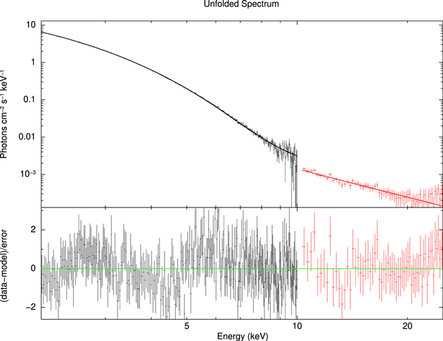
Figure 2. A representative (ObsID P011466110701) unfolded spectrum. The spectrum was rebinned just for the purpose of display.
Download figure:
Standard image High-resolution imageAs we mentioned earlier, in order to have a successful application of the continuum-fitting method, it is important to ensure a disk with the bolometric Eddington-scaled luminosity l < 0.3. For MAXI J1820+070, it is clear that our selected "gold" spectra satisfy this standard, with l ranging from 0.056 to 0.150.
3.3. Error Analysis
The errors quoted in Tables 2 and 3 are only due to the statistic uncertainties estimated via Xspec. The confidence level is 90%. As mentioned in Section 1, the error budget of a* is dominated by the combined observational uncertainties of M, i, and D. Herein the Monte Carlo (MC) simulation was performed for error analysis. The steps of error analysis are described as follows: for each individual spectrum, (1) assuming independent and Gaussian distributed, 11 we generate 3000 sets of (M, i, D). (2) we calculate look-up tables of f for these parameter sets. (3) we refit the spectrum 3000 times with these (M, i, D) to determine the histograms of a*, from which we finally decide the error of a*.
We made MC simulations on 54 "gold" spectra. Histograms of a* are plotted in Figure 3, and the summed histogram is shown in Figure 4. Adopting the histogram, we arrived at the final value of a* = 0.14 ± 0.09 (1σ).
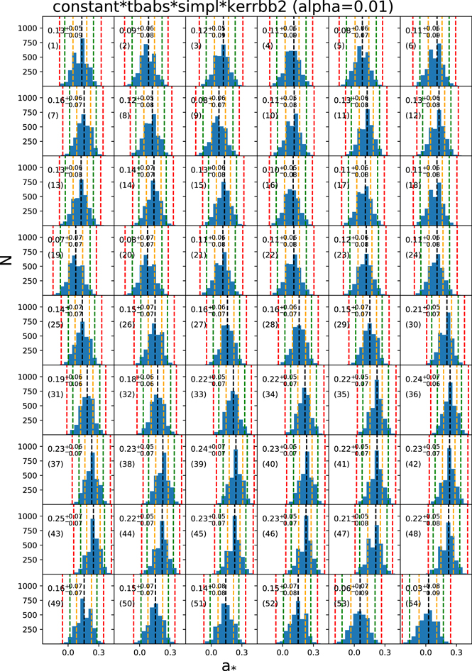
Figure 3. Histograms of a* calculated via the Monte Carlo analysis for 3000 sets of parameters per spectrum. The three dashed lines imply the 99.7% (3σ, red), 95.4% (2σ, green), and 68.3% (1σ, orange) error, respectively. The respective 68.3% confidence level on a* is indicated in each panel.
Download figure:
Standard image High-resolution image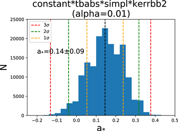
Figure 4. Summed histogram of a* for 54 spectra, including 162,000 data points.
Download figure:
Standard image High-resolution image4. Discussion
4.1. Effect of Varying Γ and Normalization
Normally we expect that if we fix the normalization of LE to 1, then the normalization of ME will also be 1. However, due to the effects of systematic errors, there are minor differences between the calibration of the two detectors (Li et al. 2020), and during the fitting process, the relative differences may change slightly (empirically, as for Insight-HXMT, within the range of 0.85–1.15 is considered as reasonable). We have tried to let the normalization vary between 0.95 and 1.05; however, it always pegs at its lower limitation 0.95 probably due to the weak Comptonization component, so we fix the normalization of ME to 0.95.
Table 5. Best-fit Parameters for Spectra with the Model constant*tbabs*simpl*kerrbb2
α = 0.01, M = 8.06 M⊙, i = 662, and D = 2.96 kpc)
| Number | ObsID | simpl | kerrbb2 | Reduced 
| χ2/d.o.f. | l | ||
|---|---|---|---|---|---|---|---|---|
| Γ | fsc | a* a |
 b
b
| |||||
| 1 | P011466108502 | 2.25 ± 0.01 | 0.1046 ± 0.0021 | −0.129 ± 0.013 | 3.63 ± 0.04 | 1.23 | 1137.9/923 | 0.173 |
| 2 | P011466108601 | 2.28 ± 0.02 | 0.0897 ± 0.0022 | −0.163 ± 0.011 | 3.86 ± 0.04 | 1.19 | 1093.1/921 | 0.181 |
| 3 | P011466108602 | 2.16 ± 0.01 | 0.0974 ± 0.0019 | −0.141 ± 0.012 | 3.73 ± 0.04 | 1.10 | 979.3/887 | 0.177 |
| 4 | P011466108702 | 2.16 ± 0.02 | 0.0572 ± 0.0018 | −0.152 ± 0.011 | 3.82 ± 0.04 | 1.10 | 918.3/835 | 0.180 |
| 5 | P011466108801 | 2.15 ± 0.02 | 0.0474 ± 0.0013 | −0.172 ± 0.007 | 3.86 ± 0.02 | 1.06 | 1043.0/980 | 0.180 |
| 6 | P011466108802 | 2.08 ± 0.02 | 0.0415 ± 0.0015 | −0.153 ± 0.009 | 3.79 ± 0.03 | 1.02 | 916.9/899 | 0.178 |
| 7 | P011466108901 | 2.04 ± 0.02 | 0.0262 ± 0.0010 | −0.079 ± 0.007 | 3.45 ± 0.02 | 0.95 | 836.3/878 | 0.168 |
| 8 | P011466109001 | 2.09 ± 0.02 | 0.0318 ± 0.0009 | −0.129 ± 0.007 | 3.65 ± 0.02 | 1.12 | 1116.2/993 | 0.174 |
| 9 | P011466109101 | 2.17 ± 0.02 | 0.0439 ± 0.0016 | −0.177 ± 0.009 | 3.80 ± 0.03 | 0.95 | 861.1/903 | 0.177 |
| 10 | P011466109102 | 2.08 ± 0.02 | 0.0355 ± 0.0011 | −0.148 ± 0.008 | 3.69 ± 0.02 | 0.99 | 912.2/923 | 0.174 |
| 11 | P011466109201 | 2.09 ± 0.02 | 0.0339 ± 0.0011 | −0.126 ± 0.009 | 3.57 ± 0.03 | 1.00 | 898.7/901 | 0.170 |
| 12 | P011466109202 | 2.10 ± 0.02 | 0.0320 ± 0.0012 | −0.122 ± 0.009 | 3.55 ± 0.03 | 1.01 | 929.1/921 | 0.170 |
| 13 | P011466109301 | 2.06 ± 0.02 | 0.0257 ± 0.0009 | −0.122 ± 0.008 | 3.53 ± 0.02 | 1.04 | 921.4/888 | 0.169 |
| 14 | P011466109401 | 2.06 ± 0.03 | 0.0211 ± 0.0009 | −0.095 ± 0.006 | 3.39 ± 0.02 | 1.02 | 918.1/896 | 0.164 |
| 15 | P011466109501 | 2.17 ± 0.02 | 0.0250 ± 0.0008 | −0.118 ± 0.007 | 3.45 ± 0.02 | 0.99 | 1002.1/1011 | 0.165 |
| 16 | P011466109503 | 2.16 ± 0.04 | 0.0338 ± 0.0019 | −0.159 ± 0.012 | 3.60 ± 0.04 | 0.92 | 679.1/741 | 0.169 |
| 17 | P011466109601 | 2.11 ± 0.02 | 0.0341 ± 0.0009 | −0.152 ± 0.007 | 3.54 ± 0.02 | 0.99 | 985.2/998 | 0.167 |
| 18 | P011466109602 | 2.11 ± 0.02 | 0.0356 ± 0.0012 | −0.153 ± 0.008 | 3.53 ± 0.02 | 1.05 | 963.9/918 | 0.166 |
| 19 | P011466109701 | 2.18 ± 0.02 | 0.0405 ± 0.0012 | −0.176 ± 0.007 | 3.54 ± 0.02 | 1.05 | 1006.0/957 | 0.165 |
| 20 | P011466109702 | 2.17 ± 0.02 | 0.0379 ± 0.0012 | −0.174 ± 0.007 | 3.52 ± 0.02 | 1.07 | 1015.4/950 | 0.164 |
| 21 | P011466109801 | 2.18 ± 0.03 | 0.0247 ± 0.0010 | −0.142 ± 0.007 | 3.35 ± 0.02 | 0.96 | 942.4/979 | 0.159 |
| 22 | P011466109802 | 2.23 ± 0.02 | 0.0278 ± 0.0010 | −0.150 ± 0.007 | 3.36 ± 0.02 | 1.04 | 1016.6/976 | 0.158 |
| 23 | P011466109803 | 2.26 ± 0.03 | 0.0260 ± 0.0012 | −0.138 ± 0.008 | 3.33 ± 0.02 | 1.01 | 970.1/960 | 0.158 |
| 24 | P011466109901 | 2.24 ± 0.03 | 0.0203 ± 0.0009 | −0.146 ± 0.007 | 3.32 ± 0.02 | 0.92 | 893.8/971 | 0.156 |
| 25 | P011466110001 | 2.50(f) | 0.0142 ± 0.0002 | −0.093 ± 0.004 | 3.09 ± 0.01 | 0.90 | 844.1/943 | 0.150 |
| 26 | P011466110101 | 2.50(f) | 0.0129 ± 0.0002 | −0.082 ± 0.004 | 2.99 ± 0.01 | 0.91 | 838.6/924 | 0.146 |
| 27 | P011466110201 | 2.50(f) | 0.0120 ± 0.0002 | −0.073 ± 0.004 | 2.90 ± 0.01 | 0.92 | 904.2/984 | 0.142 |
| 28 | P011466110301 | 2.50(f) | 0.0112 ± 0.0002 | −0.071 ± 0.004 | 2.86 ± 0.01 | 0.90 | 824.4/911 | 0.140 |
| 29 | P011466110302 | 2.50(f) | 0.0114 ± 0.0003 | −0.079 ± 0.004 | 2.88 ± 0.01 | 0.97 | 909.7/934 | 0.141 |
| 30 | P011466110401 | 2.50(f) | 0.0130 ± 0.0002 | −0.031 ± 0.005 | 2.71 ± 0.01 | 1.10 | 1040.3/947 | 0.136 |
| 31 | P011466110701 | 2.50(f) | 0.0114 ± 0.0002 | −0.044 ± 0.004 | 2.69 ± 0.01 | 1.04 | 1032.8/995 | 0.134 |
| 32 | P011466110801 | 2.50(f) | 0.0104 ± 0.0003 | −0.055 ± 0.005 | 2.69 ± 0.01 | 1.02 | 902.7/888 | 0.133 |
| 33 | P011466110901 | 2.50(f) | 0.0116 ± 0.0002 | −0.013 ± 0.006 | 2.50 ± 0.01 | 1.14 | 1078.3/945 | 0.127 |
| 34 | P011466110902 | 2.50(f) | 0.0125 ± 0.0004 | −0.007 ± 0.008 | 2.48 ± 0.02 | 0.90 | 721.1/800 | 0.126 |
| 35 | P011466111001 | 2.50(f) | 0.0149 ± 0.0003 | 0.008 ± 0.003 | 2.42 ± 0.01 | 1.15 | 1082.7/945 | 0.124 |
| 36 | P011466111201 | 2.50(f) | 0.0127 ± 0.0003 | 0.024 ± 0.004 | 2.28 ± 0.01 | 1.05 | 944.2/903 | 0.118 |
| 37 | P011466111301 | 2.50(f) | 0.0118 ± 0.0003 | 0.017 ± 0.004 | 2.27 ± 0.01 | 1.01 | 890.4/880 | 0.117 |
| 38 | P011466111401 | 2.50(f) | 0.0092 ± 0.0003 | 0.011 ± 0.004 | 2.20 ± 0.01 | 1.16 | 1045.7/900 | 0.113 |
| 39 | P011466111501 | 2.50(f) | 0.0108 ± 0.0003 | 0.028 ± 0.004 | 2.11 ± 0.01 | 1.26 | 1131.7/895 | 0.109 |
| 40 | P011466111601 | 2.50(f) | 0.0130 ± 0.0003 | 0.016 ± 0.005 | 2.05 ± 0.01 | 1.05 | 880.8/838 | 0.106 |
| 41 | P011466111701 | 2.50(f) | 0.0123 ± 0.0003 | −0.008 ± 0.008 | 2.04 ± 0.02 | 1.04 | 863.2/827 | 0.103 |
| 42 | P011466111801 | 2.50(f) | 0.0205 ± 0.0007 | 0.010 ± 0.009 | 1.93 ± 0.02 | 1.07 | 587.4/550 | 0.099 |
| 43 | P011466111802 | 2.50(f) | 0.0201 ± 0.0009 | 0.036 ± 0.017 | 1.85 ± 0.03 | 1.20 | 521.4/433 | 0.096 |
| 44 | P011466111901 | 2.50(f) | 0.0139 ± 0.0004 | 0.008 ± 0.007 | 1.85 ± 0.01 | 1.01 | 818.5/811 | 0.095 |
| 45 | P011466112001 | 2.50(f) | 0.0136 ± 0.0005 | 0.011 ± 0.006 | 1.79 ± 0.01 | 1.24 | 948.8/768 | 0.092 |
| 46 | P011466112101 | 2.50(f) | 0.0139 ± 0.0004 | 0.009 ± 0.006 | 1.73 ± 0.01 | 1.14 | 914.8/801 | 0.089 |
| 47 | P011466112201 | 2.50(f) | 0.0215 ± 0.0005 | −0.042 ± 0.011 | 1.76 ± 0.02 | 1.45 | 1064.9/734 | 0.088 |
| 48 | P011466112301 | 2.50(f) | 0.0178 ± 0.0006 | −0.016 ± 0.019 | 1.67 ± 0.03 | 1.34 | 844.2/632 | 0.084 |
| 49 | P011466112401 | 2.50(f) | 0.0202 ± 0.0005 | −0.080 ± 0.008 | 1.51 ± 0.01 | 1.25 | 966.9/772 | 0.074 |
| 50 | P011466112402 | 2.50(f) | 0.0213 ± 0.0008 | −0.083 ± 0.014 | 1.50 ± 0.02 | 0.94 | 453.8/484 | 0.073 |
| 51 | P011466112501 | 2.50(f) | 0.0247 ± 0.0004 | −0.113 ± 0.011 | 1.51 ± 0.01 | 1.29 | 1083.6/843 | 0.072 |
| 52 | P011466112601 | 2.50(f) | 0.0230 ± 0.0004 | −0.092 ± 0.007 | 1.42 ± 0.01 | 1.16 | 929.8/804 | 0.069 |
| 53 | P011466112701 | 2.63 ± 0.04 | 0.0392 ± 0.0022 | −0.232 ± 0.018 | 1.53 ± 0.02 | 1.05 | 812.1/773 | 0.069 |
| 54 | P011466112801 | 2.32 ± 0.03 | 0.0495 ± 0.0018 | −0.276 ± 0.016 | 1.52 ± 0.02 | 0.97 | 769.5/791 | 0.067 |
| 55 | P011466108401 | 2.36 ± 0.01 | 0.2581 ± 0.0022 | −0.134 ± 0.012 | 3.81 ± 0.04 | 1.66 | 1864.2/1125 | 0.181 |
| 56 | P011466108402 | 2.34 ± 0.01 | 0.2523 ± 0.0024 | −0.080 ± 0.011 | 3.67 ± 0.03 | 1.69 | 1877.8/1108 | 0.179 |
| 57 | P011466108403 | 2.38 ± 0.01 | 0.2578 ± 0.0031 | −0.170 ± 0.015 | 3.96 ± 0.04 | 1.35 | 1411.2/1044 | 0.185 |
| 58 | P011466108501 | 2.32 ± 0.01 | 0.1518 ± 0.0021 | −0.146 ± 0.012 | 3.53 ± 0.03 | 1.51 | 1542.9/1024 | 0.167 |
| 59 | P011466112901 | 2.36 ± 0.01 | 0.1588 ± 0.0018 | −0.265 ± 0.018 | 1.43 ± 0.02 | 1.24 | 1290.7/1044 | 0.064 |
| 60 | P011466113001 | 2.29 ± 0.01 | 0.1884 ± 0.0020 | −0.167 ± 0.022 | 1.18 ± 0.02 | 1.18 | 1194.8/1013 | 0.055 |
| 61 | P011466113101 | 2.17 ± 0.01 | 0.2802 ± 0.0022 | −0.146 ± 0.035 | 0.87 ± 0.03 | 1.09 | 1189.3/1087 | 0.041 |
Download table as: ASCIITypeset image
We tested the effect of different Γ and norm on a*, and the fit results are presented in Table 6. It is shown that a* decreases by △a* = 0.053 as Γ increases from 2.10 to 2.90 (with norm frozen at 0.95), and increases by △a* = 0.017 as norm varies from 0.95 to 1.05 (with Γ fix at 2.50).
Table 6. Effect of Different Γ and constant Normalization Only for P011466110701, where α = 0.01, M = 8.48 M⊙, i = 63°, and D = 2.96 kpc)
| N | Model | Parameter | Case 1 | Case 2 | Case 3 | Case 4 | Case 5 | Case 6 | Case 7 |
|---|---|---|---|---|---|---|---|---|---|
| 1 | simpl | Γ | 2.10(f) | 2.30(f) | 2.50(f) | 2.50(f) | 2.50(f) | 2.70(f) | 2.90(f) |
| 2 | simpl | fsc | 0.0058 ± 0.0001 | 0.0081 ± 0.0002 | 0.0113 ± 0.0002 | 0.0108 ± 0.0002 | 0.0101 ± 0.0002 | 0.0152 ± 0.0003 | 0.0201 ± 0.0004 |
| 3 | kerrbb2 | a* | 0.213 ± 0.002 | 0.207 ± 0.002 | 0.187 ± 0.005 | 0.190 ± 0.005 | 0.204 ± 0.002 | 0.174 ± 0.004 | 0.160 ± 0.004 |
| 4 | kerrbb2 |

| 1.99 ± 0.01 | 2.00 ± 0.01 | 2.04 ± 0.01 | 2.04 ± 0.01 | 2.01 ± 0.01 | 2.07 ± 0.01 | 2.10 ± 0.01 |
| 5 | constant | norm | 0.95(f) | 0.95(f) | 0.95(f) | 1.00(f) | 1.05(f) | 0.95(f) | 0.95(f) |
| 6 | Reduced 
| 1.21 | 1.12 | 1.04 | 1.07 | 1.11 | 0.97 | 0.91 | |
| 7 | χ2/d.o.f. | 1201.1/995 | 1118.3/995 | 1037.0/995 | 1069.5/995 | 1100.6/995 | 963.5/995 | 908.6/995 | |
| 8 | l | 0.110 | 0.110 | 0.111 | 0.111 | 0.110 | 0.112 | 0.112 |
Download table as: ASCIITypeset image
4.2. Effect of Different Parameter Configurations
As we mentioned above, the inclination is a crucial input parameter and has an obvious degeneracy with the spin. In previous section, we have estimated the spin by assuming the jet inclination angle i = 63° ± 3°, and the black hole mass M =  . We also constrained the spin for the case in which the inclination angle ranges between 662 < i < 808. Referring to Figure 5, the spin parameter decreases as the mass decreases or the inclination increases (see Section 1 for a qualitative analysis), therefore we used i = 662 and M = 8.06 M⊙ to constrain the upper limit of the spin for Torres's parameters. The fit results are shown in Table 5. The best-fit values of this set of parameters (within a range of −0.276 to 0.036 and only 11 spectra have a spin larger than zero) are lower than that of our adopted parameters, so that Torres's parameter configuration may lead to a retrograde black hole, which needs to be checked with the precise system parameters in the future. In addition, assuming M = 8.06 M⊙, the spin will peg to its lower limit −0.99 in kerrbb2 if the inclination is above 76°. The critical value of i, which will lead to a spin of −0.99, is 67° for M = 5.96 M⊙.

Figure 5. The correlation plots displaying the effect on the spin of varying M, i, and D.
Download figure:
Standard image High-resolution imageIn applying the continuum-fitting method, the inclination i is supposed to be the inclination angle of the inner disk, which, however, is hard to estimate in practice. (In the future, the X-ray polarization method may provide more accurate constraints on it.) Usually the strategy is to use the orbital inclination or jet inclination as the proxy, instead. Some previous work on fitting the reflection component reported a small misalignment between the inner accretion disk and the binary orbital plane (Fragos et al. 2010; Walton et al. 2016), which can be interpreted by a warp in the disk. In this work, we preferred the spin result for adopting the jet inclination angle as the inner disk inclination; however, more consistent and accurate dynamical parameters are required for the detailed spin measurements in the future.
As a caveat, it is noted that all the spin measurements from the continuum-fitting method (Liu et al. 2008; Gou et al. 2009, 2010, 2014; Steiner et al. 2011, 2012, 2014, 2016; Chen et al. 2016) basically suggested positive spin values, and there has been no clear observational evidence for the existence of retrograde black holes. Morningstar et al. (2014) initially reported a retrograde spin for the black hole in Nova Muscae 1991:  (90% confidence level). However, Chen et al. (2016) found a moderately high value of spin,
  (1σ confidence level) after the system parameters were updated consistently, and rule strongly against a retrograde value: a* > 0.17 (2σ or 95.4% confidence level).
5. Conclusion
In this work, we have presented a methodology of the spin measurements for the newly observed black hole X-ray binary MAXI J1820+070 using Insight-HXMT spectra. Mainly because the spin of the black hole strongly depends on the measurement of the disk inclination, the black hole mass and the distance, the large uncertainty of the dynamical parameters makes it difficult to critically evaluate its spin. For MAXI J1820+070, we have discussed two scenarios. Preferring to consider the jet inclination as the inner accretion disk inclination angle, adopting M =  , i = 63° ± 3°, and D = 2.96 ± 0.33 kpc, we deduce a value of a* = 0.14 ± 0.09 (1σ), showing that the black hole in this system is rotating slowly. Besides, when the parameter ranges 5.96 M⊙ < M < 8.06 M⊙ and 662 < i < 808 are applied, the black holes are more likely to have a retrograde spin.
Shidatsu et al. (2019) estimated the inner edge of the accretion disk in the HSS to be Rin = 77.9 ± 1.0(D/3 kpc)(cosi/cos60°)−1/2 km. Using M =  , i = 63° ± 3°, and D = 2.96 ± 0.33 kpc, the black hole in MAXI J1820+070 is nearly nonrotating, which is basically compatible with our constraint of a* = 0.14 ± 0.09 (1σ). In addition, it is noted that the reflection spectral fit to the NuSTAR prefers a smaller inner disk inclination between 30° and 40° and the spin ranges between −0.5 and 0.5 (Bharali et al. 2019; Buisson et al. 2019; Fabian et al. 2020). However, if the disk inclination is set around 70°, the spin derived from the same soft-state NuSTAR spectra would be almost maximally retrograde (a* < − 0.95, Fabian et al. 2020). In any event, we hope future observations could help improve the dynamical parameters, hence putting a tighter constraint on the spin parameters.
This work made use of the data from the Insight-HXMT mission, a project funded by China National Space Administration (CNSA) and the Chinese Academy of Sciences (CAS). The authors are thankful for support from the National Program on Key Research and Development Project (grant Nos. 2016YFA0400800 and 2016YFA0400801) and from the NSFC (U1838201 and U1838202). L.J.G. acknowledges the support by the National Program on Key Research and Development Project (grant No. 2016YFA0400804), and by the NSFC (U1838114), and by the Strategic Priority Research Program of the Chinese Academy of Sciences (XDB23040100).
Footnotes
- 6
It is noted that both the gravitational wave (Abbott et al. 2021) and Event Horizon Telescope (EHT) observations can directly constrain the black hole spin. The gravitational wave observations have provided spin constraints for tens of merging black hole systems. As for EHT, it can only resolve the event horizons for supermassive black holes rather than stellar mass black holes (Event Horizon Telescope Collaboration et al. 2019).
- 7
The radio parallax measurement of 0.348 ± 0.033 mas is consistent with the value of 0.31 ± 0.11 mas estimated by Gaia-DR2. The distance estimated from the Gaia parallax is
 kpc based on an exponentially decreasing space density prior (Gandhi et al. 2019).
 - 8
- 9
- 10
See the proposal software page in http://proposal.ihep.ac.cn/soft/soft2.jspx, and see the detailed instructions in http://proposal.ihep.ac.cn/soft/soft2help.jspx.
- 11
Previous work has confirmed that if we generate parameter sets via the mass function, the results will be roughly the same and the difference between these two methods will be nearly negligible (Zhao et al. 2020).
