


Abstract
Changing-look active galactic nuclei (AGNs) present an important laboratory to understand the origin and physical properties of the broad-line region (BLR). We investigate follow-up optical spectroscopy spanning ∼500 days after the outburst of the changing-look AGN 1ES 1927+654. The emission lines displayed dramatic, systematic variations in intensity, velocity width, velocity shift, and symmetry. Analysis of optical spectra and multiband images indicates that the host galaxy contains a pseudobulge and a total stellar mass of  . Enhanced continuum radiation from the outburst produced an accretion disk wind, which condensed into BLR clouds in the region above and below the temporary eccentric disk. Broad Balmer lines emerged ∼100 days after the outburst, together with an unexpected, additional component of narrow-line emission. The newly formed BLR clouds then traveled along a similar eccentric orbit (e ≈ 0.6). The Balmer decrement of the BLR increased by a factor of ∼4–5 as a result of secular changes in cloud density. The drop in density at late times allowed the production of He i and He ii emission. The mass of the black hole cannot be derived from the broad emission lines because the BLR is not virialized. Instead, we use the stellar properties of the host galaxy to estimate
  . The nucleus reached near or above its Eddington limit during the peak of the outburst. We discuss the nature of the changing-look AGN 1ES 1927+654 in the context of other tidal disruption events.
Export citation and abstract BibTeX RIS

Original content from this work may be used under the terms of the Creative Commons Attribution 4.0 licence. Any further distribution of this work must maintain attribution to the author(s) and the title of the work, journal citation and DOI.
1. Introduction
Broad emission lines are a hallmark characteristic of type 1 active galactic nuclei (AGNs). Arising from rapidly moving, dense photoionized gas near the supermassive black hole (BH), the emission lines from the broad-line region (BLR) are illuminated by the ultraviolet (UV) continuum from the accretion disk (e.g., Davidson & Netzer 1979; Kwan & Krolik 1981). The size of the BLR (RBLR), which can be estimated by cross-correlating the light curve of the continuum with that of the broad lines, scales with the AGN luminosity (RBLR − L correlation; e.g., Kaspi et al. 2000; Peterson et al. 2004; Bentz et al. 2013). In the classical picture, the BLR consists of a collection of clouds virialized by the gravitational potential of the central BH. This is supported by the discovery that the FWHM of broad Hβ is proportional to the radius of the BLR: FWHM (e.g., Peterson & Wandel 1999; Wang et al. 2020). Recently, a generalized BLR model was developed based on the combination of Keplerian rotation and radial motion of the clouds (Pancoast et al. 2014; Li et al. 2018). This model has been used to study the geometry of the BLR using spatially resolved interferometric spectra (Gravity Collaboration et al. 2018, 2020) and velocity-resolved reverberation mapping (RM) observations (Grier et al. 2017; Williams et al. 2018). The dynamics of the BLR may be a combination of rotation and outflow in a way that depends on the properties of individual objects (e.g., Du et al. 2016a; Horne et al. 2021).
A subset of AGNs display transient behavior in which their broad emission lines can appear or disappear, accompanied by large-amplitude continuum variability, switching between type 2 and type 1 optical classifications. Several dozens of these so-called changing-look AGNs have been discovered over the past decade (e.g., Denney et al. 2014; Shappee et al. 2014; LaMassa et al. 2015; Rumbaugh et al. 2018; MacLeod et al. 2019; Trakhtenbrot et al. 2019; Yang et al. 2019). Distinct from AGNs that exhibit dramatic X-ray variability due to varying line-of-sight (LOS) column density (e.g., Matt et al. 2003; Risaliti et al. 2006; Rivers et al. 2015; Ricci et al. 2016), optical changing-look transitions might be related to dramatic changes of the accretion flow, similar to those commonly observed in outbursting X-ray binaries (Homan & Belloni 2005; Remillard & McClintock 2006; Done et al. 2007). Observations (e.g., Ho 2008, 2009a; Noda & Done 2018; Liu et al. 2020) indicate that AGN accretion flows undergo changes in structure and radiative efficiency when the mass accretion rate ( ) reaches certain critical values relative to the Eddington accretion rate (
 ): whereas the accretion flow is geometrically thin and radiatively efficient when
  (standard thin disk; Shakura & Sunyaev 1973; Novikov & Thorne 1973), it becomes geometrically thick and radiatively inefficient when
  (slim disk; Katz 1977; Abramowicz et al. 1988; Sadowski 2009) or
  (advection-dominated accretion flow; Ichimaru 1977; Narayan & Yi 1994). Consequent changes of both the reprocessing power and covering factor of the BLR result in the appearance and disappearance of broad emission lines (Dexter et al. 2019). Large-amplitude variability of changing-look AGNs in the mid-IR further supports this picture (Sheng et al. 2017).
Alternatively, nuclear tidal disruption events (TDEs; for a review, see Gezari 2021) could also explain the sudden emergence of broad emission lines and the blue continuum (e.g., Merloni et al. 2015; Trakhtenbrot et al. 2019; Ricci et al. 2020). The central supermassive BH can accrete a fraction of the mass of the tidally disruped star, causing a flare that peaks in the extreme-UV band and that can extend to the optical and X-rays (e.g., Rees 1988; Saxton et al. 2019). TDEs can also generate highly ionized outflows, detectable as blueshifted broad hydrogen Balmer or helium lines (Miller et al. 2015; Hung et al. 2019), as well as P Cygni–like absorption features at X-ray energies (Kara et al. 2018). However, the mechanisms that produce broad emission lines in TDEs are still controversial. Observationally, broad ((1–2) × 104 km s−1) H and He lines usually dominate the spectra of optically selected TDEs (Arcavi et al. 2014). Generally observed in emission, optical lines can have complex and asymmetric shapes (e.g., Gezari et al. 2012; Arcavi et al. 2014). The width of the emission lines typically decreases with time, while the continuum luminosity drops (Holoien et al. 2016a, 2016b; Leloudas et al. 2019), opposite of what is expected from the virialized BLR of type 1 AGNs. While the unbound material from the disrupted star initially was considered to be the primary contributor to the broad emission lines (Kasen & Ramirez-Ruiz 2010; Clausen & Eracleous 2011), later hydrodynamical simulations suggest that the debris stream is confined to a negligible surface area and does not contribute significantly to either the continuum or line emission (Guillochon et al. 2014). Instead, broad emission lines may be produced in the region above and below the elliptical accretion disk. Liu et al. (2017) suggest that the optical emission lines are associated with the accretion flow, such that relativistic broadening can account for the double-peak broad Hα profile observed in some sources (e.g., Arcavi et al. 2014).
Both scenarios suggest that the accretion rate plays a role in determining the AGN type, since the optical continuum becomes bluer and brighter when changing-look AGNs turn on, and vice versa (e.g., Yang et al. 2018). It is interesting that the type 1 phase of changing-look AGNs lasts only ∼10 yr (e.g., Denney et al. 2014; McElroy et al. 2016). The variable accretion rate scenario requires that the AGN hover near the state transition threshold of  , beyond which the ionizing luminosity significantly changes. Indeed, phase-transition changing-look AGNs usually have bolometric luminosities of a few percent of LEdd (e.g., Noda & Done 2018). By contrast, the scenario involving TDEs, which can have a variety of possible penetration factors and involve diverse properties of the disrupted star, does not select BHs with a preferential
  . And while the flux can vary over a large dynamical range, the time-dependent fallback accretion rate should follow a universal form of
  (Rees 1988; Lodato & Rossi 2011). Therefore, detailed monitoring of the evolution of the BH accretion rate can, in principle, distinguish between these two scenarios.
A changing-look event was recently reported and studied (Trakhtenbrot et al. 2019; Ricci et al. 2020, 2021) in the nearby (z = 0.019422) galaxy 1ES 1927+654, a previously known type 2 (narrow-line) AGN (Boller et al. 2003; Tran et al. 2011). Following its discovery by the All-Sky Automated Survey for Supernovae (ASAS-SN; Shappee et al. 2014), its V-band flux increased by at least 2 mag in 2018 March (Nicholls et al. 2018). Subsequent optical spectroscopic follow-up spanning ∼500 days found the emergence of broad Balmer emission several weeks after the outburst, followed by broad Lyα emission detected on 2018 August 28 (Trakhtenbrot et al. 2019). This is the first case of a source whose changing-look transition has been observed.
This work studies in detail the properties of the optical lines of 1ES 1927+654, in the context of the dramatic variations of the BLR. We also constrain the mass of the BH through the properties of the host galaxy. We demonstrate that the virial mass of the BH calculated through the traditional method of assuming a virialized BLR is inconsistent with other independent estimates. Section 2 describes our photometric observations and analysis. Section 3 illustrates our optical spectral fitting and discusses the properties of the host galaxy and emission lines. We then summarize the spectral evolution of 1ES 1927+654 after the optical outburst and estimate the BH mass in Section 4. Section 5 offers a proposed physical picture of the changing-look process and evolving BLR. Conclusions are given in Section 6. For the adopted ΛCDM cosmology (Ωm = 0.308, ΩΛ = 0.692, and H0 = 67.8 km s−1 Mpc−1;Planck Collaboration et al. 2016), the luminosity distance of 1ES 1927+654 is 87.2 Mpc.
2. Photometric Analysis
The flux of the source changed significantly in the optical and UV bands following the changing-look event. Trakhtenbrot et al. (2019) provide fixed-aperture optical to UV photometry and light curves covering ∼550 days, starting from about 50 days before the outburst. To minimize contamination from foreground stars, in this study we perform imaging decomposition (Section 2.3) of the four observations acquired with the Optical/UV Monitor Telescope (OM; Mason et al. 2001) on board XMM-Newton (Jansen et al. 2001). These optical/UV images are crucial for estimating the bulge-to-total light ratio (B/T) and the stellar population of the host galaxy (Section 3.2). To constrain the total spectral energy distribution (SED) before the outburst (Section 3.2), we also follow a similar method to analyze the IR images from the Two Micron All Sky Survey (2MASS; Skrutskie et al. 2006) and the Wide-field Infrared Survey Explorer (WISE; Wright et al. 2010).
2.1. Observations
Table 1 summarizes the photometric data used in this study. We use four XMM-Newton OM observations carried out between 2011 and 2019. For each observation, we extract the original data files (ODFs). We used the omchain package in Science Operations Centre SAS v18.0.0 (Science Analysis System) for image processing, after which .SIMAGE files were generated for photometric analysis. A maximum of six filters are available (UVW2, UVM2, UVW1, U, B, V), but some epochs did not cover all of them. Near-IR (J, H, Ks ) images acquired in 1999 May 22 were downloaded from the 2MASS archives. We cut the size of the images to 10' × 10' to ensure that there is enough area for proper sky measurement. A similar size is used for the mid-IR W1−W4 images downloaded from ALLWISE (Cutri et al. 2021). A total of 68 observations of 1ES 1927+654 are available. We concentrate on those taken in 2010 June and December, which showed less than 1 mag variation.
Table 1. Summary of Photometric Analysis
| Instrument | Obs. Date | Band | FWHM | Magnitude | B/T | fAGN |

|
|---|---|---|---|---|---|---|---|
| (1) | (2) | (3) | (4) | (5) | (6) | (7) | (8) |
| 2MASS | 22-05-1999 | J | 3 11 11 | 13.99 ± 0.11 | 0.48 ± 0.06 | ⋯ | 0.656 |
| 2MASS | 22-05-1999 | H | 319 | 13.41 ± 0.35 | 0.35 ± 0.24 | ⋯ | 0.752 |
| 2MASS | 22-05-1999 | Ks | 327 | 12.86 ± 0.11 | 0.44 ± 0.06 | ⋯ | 0.943 |
| WISE | 27-06-2010 | W1 | 61 | 13.43 ± 0.55 | 0.87 ± 0.26 | ⋯ | 0.372 |
| WISE | 27-06-2010 | W2 | 68 | 12.80 ± 0.50 | 0.65 ± 0.21 | ⋯ | 0.253 |
| WISE | 27-06-2010 | W3 | 74 | 10.42 ± 0.57 | ⋯ | ⋯ | 0.277 |
| WISE | 27-06-2010 | W4 | 120 | 8.79 ± 0.63 | ⋯ | ⋯ | 0.386 |
| XMM-Newton OM | 20-05-2011 a | UVM2 | 196 | 18.62 ± 0.29 | ⋯ | ⋯ | 1.201 |
| XMM-Newton OM | 20-05-2011 | UVW1 | 214 | 17.46 ± 0.46 | 0.24 ± 0.06 | ⋯ | 1.185 |
| XMM-Newton OM | 20-05-2011 | V | 151 | 16.05 ± 0.14 | 0.30 ± 0.09 | ⋯ | 4.184 |
| XMM-Newton OM | 05-06-2018 | UVW2 | 217 | 16.45 ± 0.21 | ⋯ | > 0.90 | 2.947 |
| XMM-Newton OM | 05-06-2018 | UVM2 | 201 | 16.39 ± 0.11 | ⋯ | > 0.90 | 2.032 |
| XMM-Newton OM | 05-06-2018 | UVW1 | 249 | 16.25 ± 0.16 | ⋯ | > 0.90 | 3.816 |
| XMM-Newton OM | 05-06-2018 | U | 225 | 16.08 ± 0.44 | ⋯ | > 0.90 | 8.262 |
| XMM-Newton OM | 05-06-2018 | B | 221 | 15.99 ± 0.27 | ⋯ | > 0.90 | 12.35 |
| XMM-Newton OM | 05-06-2018 | V | 171 | 15.41 ± 0.15 | ⋯ | 0.46 ± 0.06 | 3.189 |
| XMM-Newton OM | 07-05-2019 | UVW2 | 226 | 17.58 ± 0.24 | ⋯ | > 0.90 | 9.314 |
| XMM-Newton OM | 07-05-2019 | UVM2 | 207 | 17.46 ± 0.15 | ⋯ | > 0.90 | 7.526 |
| XMM-Newton OM | 07-05-2019 | UVW1 | 258 | 17.17 ± 0.13 | ⋯ | > 0.90 | 10.28 |
| XMM-Newton OM | 07-05-2019 | U | 234 | 16.90 ± 0.20 | ⋯ | 0.81 ± 0.08 | 11.87 |
| XMM-Newton OM | 07-05-2019 | B | 201 | 16.56 ± 0.25 | ⋯ | 0.64 ± 0.07 | 20.60 |
Notes. Column (1): instrument. Column (2): date of observations. Column (3): filter. Column (4): FWHM of effective PSF, generated from field stars. Column (5): integrated magnitude of all the components. Column (6): bulge-to-total ratio. Column (7): flux fraction of the AGN component. Column (8): reduced χ2 of GALFIT model.
a For the XMM-Newton OM images, the exposure for 2011 May was 1.4 ks, while that for 2018 June was 4.5 ks and that for 2019 May was 4.4 ks.Download table as: ASCIITypeset image
2.2. Sky Subtraction and Masking
The angular diameter of 1ES 1927+654 is 2690, measured at the isophotal surface brightness level of 20 Ks
mag arcsec−2 (2MASS Extended Source Catalog; Jarrett et al. 2000). Three bright stars are located near our target of interest: star 1 (V = 13.67 mag), 1114 to the southwest; star 2 (V = 15.32 mag), 1382 to the southeast; and star 3 (V = 14.98 mag), 2297 to the southwest. The three stars, spectroscopically identified as G or K type (Boller et al. 2003), are blended with 1ES 1927+654 in all the images used here, which have a spatial resolution of FWHM > 15. We use GALFIT 3.0 to perform 2D imaging decomposition for proper deblending and photometric measurement (Section 2.3). An accurate estimation of the background, which GALFIT assumes to be uniform, is needed for the analysis. However, large-scale variations may be present in the background of real images. For instance, in the near-IR bands, particularly for the 2MASS Ks
band, "airglow" can produce a ∼200'' gradient in the background (Jarrett et al. 2000). For the XMM-Newton OM, ghost images from light scattered within the detector may be important.
10
We generate segmentation images following standard methods of source detection (e.g., SExtractor), using "sigma clipping" to estimate the rms of the background, and then adopt 3 times the sky rms as the threshold for source detection. We fit a 2D Gaussian function to convert the image segments into elliptical masks, which have the same second-order central moment as the sources. The image segments usually can be enclosed using 3 times the standard deviation of the 2D Gaussian function in the semimajor and semiminor axes. To ensure that all the emission is properly captured by the image segments, we enlarge the elliptical mask by extending its size by a factor of 2. The masks occupy more than 80% of the sky pixels in the 10' × 10' field. To model the potential large-scale background gradient, we adopt a third-order polynomial function, which is quite efficient without overfitting the faint structures of extended galaxies (Jarrett et al. 2000). We subtract the best-fit background model from the original image and use it as input for GALFIT. Sources that are not blended with 1ES 1927+654 are masked. We use SExtractor to perform preliminary source deblending, using a combination of multithresholding and watershed segmentation (Beucher & Meyer 1993). We generate the mask using the same method as that used for sky subtraction, except that we do not mask our target and the three bright foreground stars.
2.3. Imaging Decomposition
In light of the severe blending by foreground stars, it is a challenge to obtain reliable photometry for our target of interest. We simultaneously deblend 1ES 1927+654 and its three nearby stars using GALFIT, considering a 55'' box centered on our target, which is large enough to enclose all bright foreground stars while avoiding contamination from other nearby sources (Figure 1). We use the EPSFBuilder task from the Python package photutils to build the point-spread function (PSF) of each image by fitting bright, unsaturated, isolated stars in the field. We adopt a convolution box of size 40'' × 40'', which is roughly 20 times the FWHM of the PSF and is large enough to cover the wings of the PSF. Sigma images were made directly from the original data, based on the Poisson noise of each pixel, which is the quadrature sum of the contribution from the source and the local sky background (Peng et al. 2010).
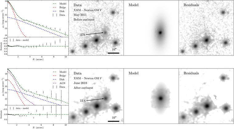
Figure 1. Example multicomponent fitting of XMM-Newton OM V-band images. Before the outburst (first row, 2011 May image), we modeled the galaxy with a Sérsic profile (bulge; red dashed curve in the first panel) plus an exponential profile (disk; blue dashed curve in the first panel). The overall model (green dashed curve in the first panel) shows good consistency with the data (black error bars). After the outburst (second row, 2018 June image), we add a point source to account for the emission from the AGN (purple dashed curve). The second column shows the observed image, the third column shows the GALFIT model, and the fourth column shows the residuals.
Download figure:
Standard image High-resolution imageWe start our fitting with the 2011 May XMM-Newton OM V-band image, not only because it has the highest resolution (PSF FWHM = 151) but also because the V-band emission at this epoch was dominated by the host galaxy. The fit takes into account several physical considerations: (1) because of the galaxy's relatively low stellar mass (M* = 3.56 × 10⁹
M⊙; Section 3.2), we do not expect a Sérsic index higher than 6 (Gao et al. 2020); (2) the axis ratio (b/a) should be higher than 0.15, since only 1% of galaxies with M* ≃ 109
M⊙ have b/a < 0.15 (Sánchez-Janssen et al. 2010); and (3) different components of the same objects should have the same central position. The best-fitting result suggests that the galaxy can be described by the sum of a Sérsic component with index n = 1.5 (effective radius re
= 042, axis ratio b/a = 0.24, position angle PA = 75 7) plus an exponential profile (re
= 683, b/a = 0.44, PA = 879). These two components are clearly evident in the 1D surface brightness profile (the first column of Figure 1) generated using the IRAF task ellipse. The compact (red dashed curve) and extended (blue dashed curve) components can be interpreted as the bulge and the disk of the host galaxy, respectively. The uncertainty of the integrated magnitude of each component follows
7) plus an exponential profile (re
= 683, b/a = 0.44, PA = 879). These two components are clearly evident in the 1D surface brightness profile (the first column of Figure 1) generated using the IRAF task ellipse. The compact (red dashed curve) and extended (blue dashed curve) components can be interpreted as the bulge and the disk of the host galaxy, respectively. The uncertainty of the integrated magnitude of each component follows

where σstat represents the statistical uncertainty, which is analytically given by GALFIT based on the covariance matrix of the parameters, and σsyst is the systematic uncertainty of our image decomposition method, which we estimate from the standard deviation of the integrated magnitudes of different bulge models with Sérsic indexes fixed from n = 1 to n = 5.
Table 1 summarizes the estimates of B/T that we deem to be reliable, in bands in which stellar emission dominates. As expected, the bulge tends to be more prominent at longer wavelengths. With B/T = 0.44 in the Ks band, the bulge of 1ES 1927+654 is about twice as dominant as other galaxies of similar mass. For example, galaxies with M* ≃ 109 M⊙ typically have B/T ≲ 0.2 (Moffett et al. 2016). The host galaxy became severely contaminated by the AGN after the outburst that triggered the changing-look event. Consequently, we add a point-source component to represent the AGN contribution for the 2018 and 2019 observations. When modeling the post-outburst images, the parameters of the host galaxy were fixed to the best-fit values before the outburst, and we only allowed the normalization to adjust. We calculate the fraction of AGN emission (fAGN) by dividing the flux of the point-source component by the total flux, and we estimate its uncertainties following Equation (1). For observations in which the central AGN dominates the total emission, the host galaxy component cannot be measured with confidence, and we simply provide a lower limit for fAGN.
3. Spectroscopic Analysis
The optical spectrum of 1ES 1927+654 acquired by Boller et al. (2003) 16 yr prior to the outburst (2017 December 23) shows prominent narrow emission lines superposed on a starlight-dominated continuum and no evidence of either Fe ii multiplets or broad lines. With [O iii] λ5007/Hβ = 14.6 and [N ii] λ6584/Hα = 0.6, the spectrum is typical of that of Seyfert 2 galaxies (Veilleux & Osterbrock 1987; Ho et al. 1993). The 26 post-outburst spectra presented by Trakhtenbrot et al. (2019) first reveal a blue continuum and, about 3 months later, broad emission lines. Together with eight additional spectra acquired after Trakhtenbrot et al. (2019), here we uniformly analyze all 34 spectra using multicomponent decomposition, separately focusing on the global spectral modeling before and after the outburst, the evolution of the broad emission lines, and their physical interpretation.
3.1. Flux Calibration
As the spectra were taken over the course of many observing runs, under a variety of conditions and using diverse instrument configurations, they must be homogenized onto a common flux scale prior to further analysis. The spectra presented in Trakhtenbrot et al. (2019) were originally scaled to match the o-band photometry of the Asteroid Terrestrial-impact Last Alert System (ATLAS; Tonry et al. 2018). However, because the effective wavelength of the o band (∼6800 Å) is contaminated by Hα, which was very bright ∼100–200 days after the outburst when a broad component surfaced, here we seek a different strategy for flux calibration. We use, instead, the flux of the [O iii] λ5007 line measured prior to the outburst as the reference for scaling the flux of the new observations, under the conventional assumption (but see Section 4.3) that the narrow-line region has remained constant over the monitoring period. Given the pre-outburst [O iii] luminosity of 2.6 × 1040 erg s−1 (Boller et al. 2003), the narrow-line region subtends a radius of ∼1 kpc according to the size–luminosity relation of Chen et al. (2019), a scale that is well captured by our later spectroscopic observations (slit widths ∼15 −2''; Trakhtenbrot et al. 2019).
3.2. Before the Outburst
The pre-outburst spectrum (Boller et al. 2003) taken in 2001 June covers 4000 − 7000 Å with a spectral resolution of 6 Å (3 pixels) and a signal-to-noise ratio (S/N) of ∼30. We first scale the absolute flux of the spectrum to match our photometric measurements from the 2011 XMM-Newton OM observation (factor 13.4 ± 2.7; Section 2.1), since at this time the optical continuum was dominated by the host galaxy and variability should be negligible on a timescale of ∼10 yr. We then correct the spectrum for a Galactic dust extinction of AV = 0.23 mag (Schlafly & Finkbeiner 2011) using the extinction curve of Cardelli et al. (1989) and convert to the rest frame assuming a redshift of z = 0.01942, which was calculated from the narrow emission lines by Trakhtenbrot et al. (2019).
We incorporate the optical spectrum into a global fit of the broadband SED (Figure 2), covering ∼2300 Å to 22.2 μm, using the Bayesian Markov Chain Monte Carlo (MCMC) inference method developed by Shangguan et al. (2018), with the primary aim of estimating the total stellar mass of the galaxy. After masking the emission lines, 11 we simultaneously fit the scaled 2001 spectrum with photometric measurements derived from the 2011 XMM-Newton OM images in the UVM2, UVW1, and V bands; 2MASS images in the J, H, and Ks bands; and WISE images in the W1, W2, W3, and W4 bands. Our model consists of three components: (1) a stellar component, represented by a Bruzual & Charlot (2003) stellar population synthesis model consisting of two simple stellar populations (SSPs) of solar metallicity, 12 with allowance for internal extinction; (2) an AGN component, represented by a power law, for scattered emission from the accretion disk, which can be substantial for type 2 AGNs (Bessiere et al. 2017; Zhao et al. 2019); and (3) a torus component, using the clumpy CAT3D torus model of Hönig & Kishimoto (2017), but without including the possible effect of a polar wind, which would be difficult to constrain with the currently limited data. The best-fit parameters are given in Table 2.

Figure 2. Optical to mid-IR SED before the outburst (Section 3.2). The black curve shows the 2001 June optical spectrum (Boller et al. 2003) scaled to match the 2011 XMM-Newton OM V-band photometry in the observed frame. Error bars show our photometric measurements of the 2011 OM images in the UVM2, UVW1, and V bands (purple); 2MASS images in the J, H, and Ks bands (green); and WISE images in the W1−W4 bands (blue). The red curve and the red shaded region show our best-fit model and its 1σ uncertainty, respectively, which consists of two SSPs (Bruzual & Charlot 2003; golden and orange curve), a featureless power-law component (green curve), and a dusty torus (Hönig & Kishimoto 2017; blue curve).
Download figure:
Standard image High-resolution imageTable 2. Best-fit Parameters before the Outburst
| Component | Parameter | Best-fit Value |
|---|---|---|
| (1) | (2) | (3) |
| Reddening | AV |

|
| SSP1 | log M* [M⊙] |

|
| t [Gyr] |

| |
| SSP2 | log M* [M⊙] |

|
| t [Gyr] |

| |
| Power law | αν |

|
| log L5100 [erg s−1] |

| |
| Torus | a |

|
| h |

| |
| N0 |

| |
| i |

| |
| log Ltorus [erg s−1] |

| |
Note. Best-fit parameters of the optical to MIR SED before the outburst (see Section 3.2). Column (1): component of the overall model. Column (2): parameter of the model and its units. Column (3): best-fit value of the parameter. Each SSP is described by its stellar mass (M*) and age (t). For the power-law AGN component, we allow the slope (αν ) and normalization (L5100) to vary. The torus component is described by five free parameters: (1) power-law index of the radial dust cloud distribution (a), (2) dimensionless scale height (h ≡ H/r), (3) number of clouds along an equatorial LOS (N0), (4) inclination angle (i), and (5) integrated luminosity (Ltorus).
Download table as: ASCIITypeset image
AGN activity was already present in 1ES 1927+654 before the outburst. From the pre-outburst 2–10 keV luminosity of L2–10 keV ≃ 2.4 × 1042 erg s−1 (Gallo et al. 2013), the empirical correlation between hard X-ray and mid-IR emission (Asmus et al. 2015) predicts a monochromatic 12 μm luminosity  , which is roughly consistent with our photometric measurements in the W3 band (
 ), especially considering the nonsimultaneity of the X-ray and mid-IR observations.
The host galaxy stellar mass helps to constrain the BH mass (Section 4.6). From the 2D image analysis (Table 1), the integrated Ks
-band luminosity of 1ES 1927+654 is  . Considering the rest-frame color (B − V)0 = 0.42 mag calculated from the 2001 optical spectrum, we infer a mass-to-light ratio M/LK
= 0.32 (scatter 0.05 dex) following the relation reported in Kormendy & Ho (2013), or
. Considering the rest-frame color (B − V)0 = 0.42 mag calculated from the 2001 optical spectrum, we infer a mass-to-light ratio M/LK
= 0.32 (scatter 0.05 dex) following the relation reported in Kormendy & Ho (2013), or  , a factor of ∼2 larger than the total stellar mass derived from our SED fitting (
 Table 2). This level of disagreement is not unexpected when comparing current stellar population synthesis models in the optical and near-IR (Baldwin et al. 2018), a problem that is also evident in the systematic mismatch of the 2MASS points in our SED fit (Figure 2). The low stellar mass of the host galaxy of 1ES 1927+654—comparable to that of the Large Magellanic Cloud (2.7 × 10⁹
M⊙; van der Marel et al. 2002)—suggests that its bulge (Section 2.1) likely belongs to the pseudobulge variety (Kormendy & Kennicutt 2004). According to Gao et al. (2020), this holds for all bulges hosted by galaxies with M* ≃ 108.5–109.5
M⊙ in the Carnegie-Irvine Galaxy Survey (Ho et al. 2011), as well as for most galaxies of similarly blue optical colors (B − V = 0.4 mag; Gao et al. 2020) and bulge Sérsic indices (n ≃ 1.5; Gao et al. 2019). We conclude that 1ES 1927+654 likely hosts a pseudobulge.
Table 2). This level of disagreement is not unexpected when comparing current stellar population synthesis models in the optical and near-IR (Baldwin et al. 2018), a problem that is also evident in the systematic mismatch of the 2MASS points in our SED fit (Figure 2). The low stellar mass of the host galaxy of 1ES 1927+654—comparable to that of the Large Magellanic Cloud (2.7 × 10⁹
M⊙; van der Marel et al. 2002)—suggests that its bulge (Section 2.1) likely belongs to the pseudobulge variety (Kormendy & Kennicutt 2004). According to Gao et al. (2020), this holds for all bulges hosted by galaxies with M* ≃ 108.5–109.5
M⊙ in the Carnegie-Irvine Galaxy Survey (Ho et al. 2011), as well as for most galaxies of similarly blue optical colors (B − V = 0.4 mag; Gao et al. 2020) and bulge Sérsic indices (n ≃ 1.5; Gao et al. 2019). We conclude that 1ES 1927+654 likely hosts a pseudobulge.
The two SSPs both have best-fit ages less than 1 Gyr, suggesting that 1ES 1927+654 has undergone a recent starburst. The majority of post-starburst galaxies in the mass range M* ≈ 109.5–1010.5 M⊙ have experienced a disruptive event such as a gas-rich major merger (Pawlik et al. 2018), which may help explain 1ES 1927+654's somewhat unusually large B/T (Section 2.3). It would also reinforce the argument that this changing-look event is associated with a TDE (Trakhtenbrot et al. 2019), which preferentially occur in post-starburst environments (Arcavi et al. 2014).
3.3. After the Outburst
The presence of a featureless blue continuum and broad Balmer lines after the optical outburst indicates that 1ES 1927+654 changed from a type 2 to a type 1 AGN. Among the 34 optical spectra available, 31 have full wavelength coverage from 4000 to 8000 Å, while the earliest three spectra covered only 4000–6700 Å and did not include the entire Hα profile. The detailed analysis of the spectra in this phase requires a different approach from that used for the spectrum before the outburst (Section 3.2). The primary aim is to quantify the evolution of the featureless continuum and broad emission lines, including their luminosities and shapes. We also use this information to estimate the virial BH mass (MBH; Section 4.6).
The overall continuum must be modeled and subtracted prior to analyzing the emission lines. After correcting for Galactic extinction and shifting to the rest frame, we construct a model for the continuum comprising (1) a power law for the accretion disk emission; (2) broad, blended iron emission; and (3) starlight from the host galaxy (Figure 3). For the power-law component, we allow its slope and normalization to vary for each spectrum. For the iron lines, we adopt the empirical template derived from observations of I Zw 1 (Boroson & Green 1992), which covers the wavelength range ∼3560–7500 Å, adjusting its normalization and FWHM but not its radial velocity shift relative to the systemic velocity of the galaxy (Hu et al. 2008, 2012). Contrary to common practice (e.g., Ho et al. 2012), here we do not consider the Balmer continuum because it contributes negligibly at wavelengths longer than 4000 Å. The host galaxy contribution comes directly from the results of Section 3.2. The emission of 1ES 1927+654 prior to the outburst was dominated by the host galaxy, which is given by the best-fitting SSP components in Table 2. We allow the normalization to change, since different spectra admit different relative fractions of host galaxy light, depending on the aperture size and seeing conditions. The continuum model, fit over several line-free windows (4435−4700 Å, 5100−5535 Å, 6000−6150 Å, and 7000−7600 Å), is illustrated in Figure 3.

Figure 3. Illustration of optical continuum fitting, using as an example the spectrum acquired on 2018 April 24. The continuum model consists of an AGN power-law component (green), broad iron emission (purple), and host galaxy starlight (cyan). The overall model (black) reproduces well the spectrum in the four fitting windows shown with gray shaded regions.
Download figure:
Standard image High-resolution imageThe emission-line fits consider nearly all the standard optical diagnostic narrow forbidden lines, including [O iii] λ λ4959, 5007, [O i] λ λ6300, 6364, [N ii] λ λ6548, 6584, and [S ii] λ λ6716, 6731, as well as the permitted lines of He ii λ4686, He i λ5877, Hγ, Hβ, and Hα, which can have both a broad and a narrow component. Although the first-order global continuum has been removed, the regions surrounding some weak emission lines (e.g., Hγ or He i) need to be adjusted using a local power-law continuum to achieve a satisfactory fit. The narrow components of Hα or Hβ are especially troublesome because they are severely blended with their broad counterparts. Following standard practice (e.g., Ho et al. 1997; Ho & Kim 2009), we use a nearby, relatively unblended narrow forbidden line as an empirical profile template, namely, [O iii] in the case of Hβ and, if sufficiently strong, [S ii] in the case of the Hα+[N ii] complex. We fix the wavelength separation of the doublets to their laboratory values and the relative amplitudes in the case of transitions that originate from the same energy level (Storey & Zeippen 2000). As the emission lines can have complex shapes (e.g., [O iii] often shows an asymmetric blue wing; Greene & Ho 2005a), we fit them with as many Gaussian components as necessary to achieve clean residuals. In practice, two Gaussians usually suffice for the narrow lines, and three for the broad ones. The narrow and broad components do not need to share the same centroid. We construct the model using the Python package lmfit and implement the fit using the MCMC method through the Python package emcee. Finally, the best-fit values and the 1σ uncertainties are calculated from the median and the 16% and 84% values.
To study quantitatively the evolution of the line profiles, we calculate the velocity shift (ΔV) of each component by integrating the first moment of the flux (∫λ fλ d λ) with respect to the median wavelength (MED) of the narrow component, where MED is defined as the location that divides the line flux equally on both sides. We integrated the first moment over 5 times the median absolute deviate, MAD = ∫∣λ −MED∣fλ d λ /∫fλ d λ. For the broad components of Hα and Hβ, we also compute the symmetry parameter

where x is the velocity centered on the integrated first moment of the profile, while f(x) is the modeled flux density,  is the symmetric part of the profile, and
  is the antisymmetric part. The norm of the profile is ∥f(x)∥ = ∫∣f(x)∣dx. The basic properties of the emission lines are summarized in Table 3.
Table 3. Properties of the Emission Lines
| Date | logL5100 |
![$\mathrm{log}{L}_{[{\rm{O}}\,\mathrm{III}]}$](https://content.cld.iop.org/journals/0004-637X/933/1/70/revision1/apjac714aieqn32.gif)
|

|

| FWHM
|

|

|

|

| FWHM
|

|

|

|

|

|

|
|---|---|---|---|---|---|---|---|---|---|---|---|---|---|---|---|---|
| (erg s−1) | (erg s−1) | (erg s−1) | (erg s−1) | (km s−1) | (km s−1) | (erg s−1) | (erg s−1) | (km s−1 ) | (km s−1 ) | (erg s−1 ) | (erg s−1 ) | (erg s−1 ) | (erg s−1 ) | |||
| (1) | (2) | (3) | (4) | (5) | (6) | (7) | (8) | (9) | (10) | (11) | (12) | (13) | (14) | (15) | (16) | (17) |
| 06-03-2018 |

|

|

|

|

|

|

|

|

|

|

|

| ≤39.22 | ≤40.22 | ≤09 | ≤39.87 |
| 08-03-2018 |

|

|

|

|

|

|

|

|

|

|

|

| ≤38.88 | ≤39.87 | ≤38.73 | ≤39.52 |
| 09-03-2018 |

|

|

|

|

|

|

|

|

|

|

|

| ≤39.88 | ≤40.88 | ≤39.67 | ≤40.46 |
| 13-03-2018 |

|

|

|

|

|

|

|

|

|

|

|

| ≤39.78 | ≤40.94 | ≤39.72 | ≤40.61 |
| 23-03-2018 |

|

|

|

|

|

|

|

|

|

|

|

| ≤40.30 | ≤41.31 | ≤40.21 | ≤41.01 |
| 23-04-2018 |

|

|

|

|

|

|

|

|

|

|

|

| ≤40.59 | ≤41.60 |

|

|
| 24-04-2018 |

|

|

|

|

|

|

|

|

|

|

|

| ≤39.32 | ≤40.34 |

|

|
| 07-05-2018 |

|

|

|

|

|

|

|

|

|

|

|

| ≤41.06 | ≤42.07 |

|

|
| 14-05-2018 |

|

|

|

|

|

|

|

|

|

|

|

| ≤40.98 | ≤41.99 |

|

|
| 28-05-2018 |

|

|

|

|

|

|

|

|

|

|

|

| ≤40.78 | ≤41.79 |

|

|
| 03-06-2018 |

|

|

|

|

|

|

|

|

|

|

|

| ≤41.07 | ≤42.07 |

|

|
| 11-06-2018 |

|

|

|

|

|

|

|

|

|

|

|

| ≤40.65 | ≤41.66 |

|

|
| 13-06-2018 |

|

|

|

|

|

|

|

|

|

|

|

| ≤39.47 | ≤40.50 |

|

|
| 24-06-2018 |

|

|

|

|

|

|

|

|

|

|

|

| ≤39.41 | ≤40.43 |

|

|
| 28-06-2018 |

|

|

|

|

|

|

|

|

|

|

|

| ≤39.63 | ≤40.64 |

|

|
| 06-07-2018 |

|

|

|

|

|

|

|

|

|

|

|

| ≤39.47 | ≤40.48 |

|

|
| 16-07-2018 |

|

|

|

|

|

|

|

|

|

|

|

| ≤38.93 | ≤39.94 |

|

|
| 17-07-2018 |

|

|

|

|

|

|

|

|

|

|

|

| ≤39.30 | ≤40.31 |

|

|
| 27-07-2018 |

|

|

|

|

|

|

|

|

|

|

|

| ≤40.31 | ≤41.31 |

|

|
| 11-08-2018 |

|

|

|

|

|

|

|

|

|

|

|

| ≤39.54 | ≤40.55 |

|

|
| 12-08-2018 |

|

|

|

|

|

|

|

|

|

|

|

| ≤39.64 | ≤40.65 |

|

|
| 08-09-2018 |

|

|

|

|

|

|

|

|

|

|

|

| ≤39.85 | ≤40.86 |

|

|
| 13-11-2018 |

|

|

|

|

|

|

|

|

|

|

|

| ≤40.45 | ≤41.47 |

|

|
| 19-03-2019 |

|

|

|

|

|

|

|

|

|

|

|

| ≤39.57 | ≤40.58 |

|

|
| 06-04-2019 |

|

|

|

|

|

|

|

|

|

|

|

|

|

|

|

|
| 19-05-2019 |

|

|

|

|

|

|

|

|

|

|

|

|

|

|

|

|
| 08-06-2019 |

|

|

|

|

|

|

|

|

|

|

|

|

|

|

|

|
| 19-06-2019 |

|

|

|

|

|

|

|

|

|

|

|

|

|

|

|

|
| 30-06-2019 |

|

|

|

|

|

|

|

|

|

|

|

|

|

|

|

|
| 03-07-2019 |

|

|

|

|

|

|

|

|

|

|

|

|

|

|

|

|
| 25-07-2019 |

|

|

|

|

|

|

|

|

|

|

|

|

|

|

|

|
| 18-08-2019 |

|

|

|

|

|

|

|

|

|

|

|

|

|

|

|

|
| 19-08-2019 |

|

|

|

|

|

|

|

|

|

|

|

|

|

|

|

|
| 10-09-2019 |

|

|

|

|

|

|

|

|

|

|

|

|

|

|

|

|
Note. Properties of the emission lines obtained from the MCMC fitting (Section 3.3). Column (1): date of observations. Column (2): monochromatic continuum luminosity at 5100 Å. Column (3): luminosity of [O iii] λ5007. Columns (4)–(5): luminosity of the narrow and broad components of Hβ. Columns (6)–(8): FWHM, velocity shift, and symmetry of broad Hβ. Columns (9)–(10): luminosity of the narrow and broad components of Hα. Columns (11)–(13): FWHM, velocity shift, and symmetry of broad Hα. Columns (14)–(15): luminosity of the narrow and broad components of He ii λ4686. Columns (16)–(17): luminosity of the narrow and broad components of He i λ5877.
Only a portion of this table is shown here to demonstrate its form and content. A machine-readable version of the full table is available.
Download table as: DataTypeset image
4. Spectral Evolution
4.1. Optical Continuum
The properties of the intrinsic AGN optical continuum,  , can be summarized with the evolution of the monochromatic luminosity at 5100 Å, L5100 ≡ λ
Lλ
(5100 Å), and the spectral index αν
. In sharp contrast to the behavior of the X-ray light curve, which decreases from the time of the outburst until ∼200 days and then rebounds (Ricci et al. 2020, 2021), L5100, consistent with the optical photometric light curve (Trakhtenbrot et al. 2019), drops monitonically with time approximately as t−5/3 (Figure 4(a)). A disk with a temperature profile T ∝ r−p
produces a spectrum fν
∝ ν3−2/p
. For a standard optically thick, geometrically thin accretion disk (Shakura & Sunyaev 1973), p = 3/4 and αν
= 1/3, whereas in a slim disk p = 1/2 and αν
= −1 (Kato et al. 2008). At the beginning of our spectral series, the value of αν
indeed roughly matches that expected for a standard thin disk (Figure 4(b)). During the nearly 600 days spanned by our observations, the spectral index gradually decreases to a final value of αν
≈ −0.3 to −0.4 (Figure 4), close to that measured from the Sloan Digital Sky Survey (SDSS) composite spectrum of quasars (αν
= −0.44; Vanden Berk et al. 2001). Interestingly, at t ≈ 200 days since the optical outburst, αν
quickly dropped from the value expected for a standard disk to that observed in SDSS quasars, closely tracking the sharp minimum reached in the X-ray light curve. Since αν
is determined by the temperature profile of the disk, the drop at t ≈ 200 suggests that the T ∝ r−p
dependence temporarily became shallower than that of the standard disk solution. The broadband SED analysis of 1ES 1927+654 by Li et al. (2022) suggests that efficient cooling suppressed the temperature of the inner disk, resulting in a shallower disk temperature profile and hence αν
.
, can be summarized with the evolution of the monochromatic luminosity at 5100 Å, L5100 ≡ λ
Lλ
(5100 Å), and the spectral index αν
. In sharp contrast to the behavior of the X-ray light curve, which decreases from the time of the outburst until ∼200 days and then rebounds (Ricci et al. 2020, 2021), L5100, consistent with the optical photometric light curve (Trakhtenbrot et al. 2019), drops monitonically with time approximately as t−5/3 (Figure 4(a)). A disk with a temperature profile T ∝ r−p
produces a spectrum fν
∝ ν3−2/p
. For a standard optically thick, geometrically thin accretion disk (Shakura & Sunyaev 1973), p = 3/4 and αν
= 1/3, whereas in a slim disk p = 1/2 and αν
= −1 (Kato et al. 2008). At the beginning of our spectral series, the value of αν
indeed roughly matches that expected for a standard thin disk (Figure 4(b)). During the nearly 600 days spanned by our observations, the spectral index gradually decreases to a final value of αν
≈ −0.3 to −0.4 (Figure 4), close to that measured from the Sloan Digital Sky Survey (SDSS) composite spectrum of quasars (αν
= −0.44; Vanden Berk et al. 2001). Interestingly, at t ≈ 200 days since the optical outburst, αν
quickly dropped from the value expected for a standard disk to that observed in SDSS quasars, closely tracking the sharp minimum reached in the X-ray light curve. Since αν
is determined by the temperature profile of the disk, the drop at t ≈ 200 suggests that the T ∝ r−p
dependence temporarily became shallower than that of the standard disk solution. The broadband SED analysis of 1ES 1927+654 by Li et al. (2022) suggests that efficient cooling suppressed the temperature of the inner disk, resulting in a shallower disk temperature profile and hence αν
.

Figure 4. Evolution of (a) optical monochromatic luminosity at 5100 Å (black points with error bars; left axis) and X-ray luminosity (green curve; right axis) and (b) optical spectral index after the outburst (Section 3.3). The x-axis is in days since the optical outburst (2017 December 23). The optical light curve agrees well with a ∼ t−5/3 trend (dashed line). The X-ray light curve, derived from NICER observations (Ricci et al. 2020, 2021), is rebinned as the median luminosity every 10 days, and the green shaded region delimits the corresponding minimal and maximal luminosity. In panel (b), the dashed line denotes the spectral index αν ≃ − 0.44 derived from the composite spectrum of SDSS quasars (Vanden Berk et al. 2001). The dotted line shows the spectral index αν ≃ 0.33 predicted by a standard accretion disk (Shakura & Sunyaev 1973). The colored boxes in both panels highlight the four epochs illustrated in Figures 5 and 7.
Download figure:
Standard image High-resolution image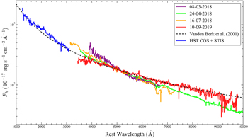
Figure 5. Example of continuum fitting of the optical spectra obtained after the outburst (Section 3.3). We show spectra taken in four epochs, normalized at 5100 Å and after subtracting the emission lines, together with the HST COS and STIS UV spectrum acquired on 2018 August 28 (blue). The four epochs illustrated here correspond to the colored boxes in Figure 4, as well as the emission-line fits in Figure 7. All the spectra are median rebinned to 10 Å pixel−1. The black dashed line represents the power-law fit of the composite spectrum of SDSS quasars (Vanden Berk et al. 2001).
Download figure:
Standard image High-resolution image4.2. Behavior of the Broad Balmer Lines
Broad Hα and Hβ are weak but visible in our very first spectrum acquired on 2018 March 6, ∼80 days after the fiducial outburst date of 2017 December 23. Both lines rose sharply to a maximum that extends from ∼120 to 230 days, with the luminosity of Hα reaching ∼2 × 1041 erg s−1 (Figure 6(a)). The optical continuum reached its maximum considerably earlier, at approximately 50 days at ∼6800 Å (o band of ATLAS), nearly 1–3 months before the first appearance of the broad emission lines (Trakhtenbrot et al. 2019). With L5100 ≈ (1–3) × 1043 erg s−1 during the first 200 days (Figure 4(a)), 1ES 1927+654 should exhibit a line-to-continuum lag of ∼10–16 days according to the RBLR − L5100 relation (Bentz et al. 2013), or even less if the source is super-Eddington (Du et al. 2016b). The large disparity between this expected lag and the actually observed time lag suggests that the BLR was formed just after the changing-look event and is probably not yet virialized.

Figure 6. Light curves for Hα (red), Hβ (blue), and Hγ (magenta; detections with S/N > 3), for (a) the broad component and (b) the narrow component. The x-axis is in days since the optical outburst (2017 December 23). The nondetections (upper limits) for Hγ are shown as magenta triangles, where only the median value is plotted and the range is shown as a shaded region. The dashed lines mark the luminosity of narrow Hα (red) and Hβ (blue) luminosity before the optical burst (Boller et al. 2003). All the light curves are normalized based on the median [O iii] luminosity.
Download figure:
Standard image High-resolution imageThe most dramatic manifestation of the dynamically evolving nature of the BLR in 1ES 1927+654 comes from the kinematics of the broad lines. Figure 7 illustrates the evolution of the line profiles, from the first epoch for which we have data (2018 March 8) to the last observation of our campaign (2019 September 10). The profile evolution can be divided into four stages:
- 1.After their emergence around 2018 March 8, the broad components of Hα and Hβ were weak. Both lines have a similar blueshift, and possibly a similar profile, although the low S/N of the lines compel us to keep the two profiles fixed during the fit.
- 2.As the strength of broad Hα and Hβ increased around 2018 April 24, their velocity profiles started to diverge. We use three Gaussian components to achieve a good fit. Hα is notably more blueshifted and blue asymmetric compared to Hβ.
- 3.Then, on 2018 July 16, Hα and Hβ were still strong, and the lines have significantly different profiles and, notably, have shifted to positive velocities.
- 4.By 2019 September 10, both Hα and Hβ have become weaker, and He ii λ4686, which has both a broad and narrow component, has emerged. Broad Hα and Hβ are still redshifted, but their line profiles are quite similar. To better constrain the fit, for the epochs in which broad Hβ was weak, we fixed its profile to that of broad Hα.
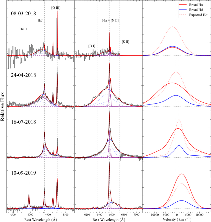
Figure 7. Analysis of the emission lines in the Hβ and Hα regions for spectra obtained on 2018 March 8, 2018 April 24, 2018 July 16, and 2019 September 10, where the 2018 March 8 spectrum has been median binned to 5 Å pixel−1 to reduce the noise (for the purposes of the display). The black curve shows the original data, the blue curves represent broad-line components, and the purple curves represent narrow-line components, with individual subcomponents further delineated with Gaussians in dashed lines. Prominent emission lines are labeled. The right column shows the best-fit velocity profile of the broad components of Hα (solid red curve) and Hβ (solid blue curve), while the dashed red curve denotes the expected Hα line if it had the same profile as Hβ but with a flux 3.05 times larger, which corresponds to a typical line ratio between Hα and Hβ (Osterbrock & Ferland 2006). The black vertical dashed–dotted line marks zero velocity shift.
Download figure:
Standard image High-resolution imageWe turn next to the velocity shift (ΔV) of the broad lines as a function of time (Figure 8(a)). The broad Hα line is first blueshifted ( ) and then redshifted (
 ) ∼300 days after the event is thought to have started. Broad Hβ generally has similar ΔV to broad Hα, with the largest discrepancy between the two found at ∼200 days, as is already evident from the spectral fits in Figure 7 (see second and third rows). We try to interpret the evolution of ΔV with a simple Keplerian radial velocity function. Assuming that the evolution is due to the dynamical motion of the emitting clouds,
where vr
is the radial velocity of the clouds; G is the gravitational constant, a and e are the semimajor axis and the eccentricity of the orbit, respectively;  is the true anomaly as a function of time, with t0 the initial time and t the rest-frame time; i is the inclination of the orbit with respect to the observer; and ψ is the longitude of the periapse. We first fix the inclination angle to i = 80° to minimize parameter degeneracy.
13
Fixing MBH = 1.38 × 10⁶
M⊙ estimated from the MBH − Mbulge relation (Section 4.6), we use an MCMC method to fit the model, which has free parameters t0, a, e, and ψ, to the observed ΔV of the broad Hα component.
14
The resulting highly eccentric orbit, with
is the true anomaly as a function of time, with t0 the initial time and t the rest-frame time; i is the inclination of the orbit with respect to the observer; and ψ is the longitude of the periapse. We first fix the inclination angle to i = 80° to minimize parameter degeneracy.
13
Fixing MBH = 1.38 × 10⁶
M⊙ estimated from the MBH − Mbulge relation (Section 4.6), we use an MCMC method to fit the model, which has free parameters t0, a, e, and ψ, to the observed ΔV of the broad Hα component.
14
The resulting highly eccentric orbit, with  ,
,  lt-days (∼8500 Rg
),
lt-days (∼8500 Rg
),  , and
, and  , covers most of our data points within the 1σ uncertainty (gray shaded region in Figure 8(a)). However, the orbital timescale we obtained is
  days, about twice as long as the duration of our observations. Therefore, this picture can be confirmed by future spectroscopic observations.
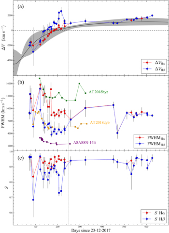
Figure 8. Evolution of (a) the velocity shift (ΔV), (b) FWHM, and (c) symmetry parameter (S; Equation (2)) of broad Hα (red) and Hβ (blue). The x-axis is in days since the optical outburst (2017 December 23). The 1σ errors associated with ΔV, FWHM, and S are calculated based on an MCMC method. In panel (a), the overall evolutionary trend was fitted with the Keplerian radial velocity function described by Equation (3), and the best-fit model and its 1σ uncertainty are plotted as the black curve and gray shaded region, respectively. In panel (b), the squares show the evolution of FWHM for Hα for TDE ASASSN-14li (purple; Holoien et al. 2016a), AT 2018dyb (orange; Leloudas et al. 2019), and AT 2018hyz (green; Short et al. 2020). We have shifted the data so that they peak at the same location as 1ES 1927+654 (∼110 days). The vertical dotted line marks 250 days after the outburst.
Download figure:
Standard image High-resolution imageThe FWHM of Hβ and Hα generally decreases with time (Figure 8(b)). Interestingly, the luminosity of the optical continuum also follows a similar trend (Figure 4). This is inconsistent with what is typically observed in type 1 AGNs, wherein  (Bentz et al. 2013). A decrease in both the continuum luminosity and the line width is often seen in TDEs, attributed to a decelerating outflow (Yang et al. 2013). For comparison, we overplot the evolution of the FWHM of Hα for the well-known TDEs ASASSN-14li (purple; Holoien et al. 2016a), AT 2018dyb (orange; Leloudas et al. 2019), and AT 2018hyz (green; Short et al. 2020), which all have period of broad Hα emission detection >100 days after the outburst. To better compare the evolution timescale, we match them to peak at the same location as the Hα FWHM of 1ES 1927+654 (∼110 days). The FWHM of Hα of 1ES 1927+654 dropped from 16,000 km s−1 to half of its maximum (∼8000 km s−1) in roughly 100 days. This is longer than the ∼50 days it took ASASSN-14li to reach its half-maximum, but the value may be underestimated since the observations of ASASSN-14li did not catch the first phase of the Hα profile variations. In spite of their quite different widths, the decreasing timescale of AT 2018dyb and AT 2018hyz appears consistent with that of 1ES 1927+654. More interestingly, all three exhibit an "echo" of increasing FWHM after ∼250 days, which may be related to the lifetime of the clouds (see Section 5.2). For Hβ, it should be noted that while its early- and late-time profiles are roughly similar to those of Hα, from ∼140 to 250 days Hβ is markedly narrower and more asymmetric (Figure 8(c)) compared to Hα. A physical picture to explain the above phenomenon is presented in Section 5.2. Prior to ∼250 days, the clouds were actively being formed. BLR clouds with different radial velocity may have different ionization state and density, leading to the production of different fractions of broad Hα and Hβ.
4.3. Variability of the Narrow Emission Lines
Figure 6(b) reveals a surprising finding: the narrow components of Hα and Hβ vary. Relative to the historic luminosity of LHα = 7.3 × 1039 erg s−1 and LHβ = 1.8 ×1039 erg s−1 (Boller et al. 2003), during the outburst the narrow components of both Hα and Hβ increased systematically by as much as a factor of 4 after 200 days, and then gradually declined, although by the end of the last epoch monitored the flux had not yet returned to its pre-outburst level. It is notable that the light curves for the narrow lines rise and fall more gradually than those of the broad lines (Figure 6(a)). The detection of variable narrow-line emission further attests to the complex kinematics and physical conditions of the dynamically evolving debris created in the aftermath of the accretion event that triggered the changing-look event (Section 5.2). Interestingly, TDE ASASSN-18pg also showed additional narrow Hα emission that emerged and evolved more slowly than the broad component of Hα (Holoien et al. 2020). However, if narrow Hα and Hβ vary, it is possible that [O iii] also varies, which would compromise our relative flux calibration strategy that assumes [O iii] to be constant (Section 3.1). We cannot resolve this uncertainty with our present data set, but we point out that our calibration assumption places a strict lower limit on the actual level of intrinsic flux variations reported in this paper.
4.4. Balmer Decrement
Our line decomposition affords us an opportunity to track the time variation of the Balmer decrement (Figure 9). During the course of the monitoring campaign, the narrow components of Hα and Hβ have a ratio between 2 and 3. The Balmer decrement of the narrow component remains constant at a value consistent with case  recombination for low-density photoionized gas (Hα/Hβ = 3.05; Osterbrock & Ferland 2006). The broad component of the Balmer lines behaves differently. While initially (Hα/Hβ)b
is substantially lower than 3.05, perhaps even as low as ∼1, after ∼200 days it increases much more dramatically with time: (Hα/Hβ)b
= (3.00 ± 0.52) × (t/500 days) + (1.93 ± 0.34) (blue points, curve, and shaded region). By the end of our campaign, (Hα/Hβ)b
≈ 5, significantly higher than the case
recombination for low-density photoionized gas (Hα/Hβ = 3.05; Osterbrock & Ferland 2006). The broad component of the Balmer lines behaves differently. While initially (Hα/Hβ)b
is substantially lower than 3.05, perhaps even as low as ∼1, after ∼200 days it increases much more dramatically with time: (Hα/Hβ)b
= (3.00 ± 0.52) × (t/500 days) + (1.93 ± 0.34) (blue points, curve, and shaded region). By the end of our campaign, (Hα/Hβ)b
≈ 5, significantly higher than the case  value attained by the narrow lines (see the trend also in the third column of Figure 7). We believe that the systematic time variation of (Hα/Hβ)b
and the large values it presents at late times are not a trivial consequence of LOS reddening by dust, which, in any case, appears negligible from the Balmer decrement of the narrow lines. Instead, the steepening of the Balmer decrement of the broad lines may reflect a decrease of both the evolving density of the clouds and the ionizing photons. From theoretical considerations, a Balmer decrement as low as ∼1 may arise under conditions of very high densities (nH > 1012 cm−3; Korista & Goad 2004). Under such conditions, the finite number of scatterings between energy levels 3 and 4 of the hydrogen atom and Lyβ leakage act to suppress the Hα intensity, leading to low (Hα/Hβ)b
(Netzer 1975). However, such a low flux ratio disappears after 150 days for all velocities (third column of Figure 7), suggesting that the clouds newly formed during this phase were not as dense as those in earlier epochs. At the other extreme, very high values of the Balmer decrement for the broad lines (∼5) can be attained at late times after the ionizing photon density drops sufficiently low (nγ
≈ 5 × 107 cm−3; Korista & Goad 2004), resulting in larger Lyα optical depth and hence a steepening of the Balmer decrement (Netzer 1975; Rees et al. 1989).
value attained by the narrow lines (see the trend also in the third column of Figure 7). We believe that the systematic time variation of (Hα/Hβ)b
and the large values it presents at late times are not a trivial consequence of LOS reddening by dust, which, in any case, appears negligible from the Balmer decrement of the narrow lines. Instead, the steepening of the Balmer decrement of the broad lines may reflect a decrease of both the evolving density of the clouds and the ionizing photons. From theoretical considerations, a Balmer decrement as low as ∼1 may arise under conditions of very high densities (nH > 1012 cm−3; Korista & Goad 2004). Under such conditions, the finite number of scatterings between energy levels 3 and 4 of the hydrogen atom and Lyβ leakage act to suppress the Hα intensity, leading to low (Hα/Hβ)b
(Netzer 1975). However, such a low flux ratio disappears after 150 days for all velocities (third column of Figure 7), suggesting that the clouds newly formed during this phase were not as dense as those in earlier epochs. At the other extreme, very high values of the Balmer decrement for the broad lines (∼5) can be attained at late times after the ionizing photon density drops sufficiently low (nγ
≈ 5 × 107 cm−3; Korista & Goad 2004), resulting in larger Lyα optical depth and hence a steepening of the Balmer decrement (Netzer 1975; Rees et al. 1989).

Figure 9. Evolution of the Balmer decrement for narrow Hα/Hβ (red) and broad Hα/Hβ (blue), as derived from our MCMC analysis, where only measurements with S/N > 3 are shown. A linear fit to the broad lines gives (Hα/Hβ)b
= 3.00 × (t/500 days) + 1.93 (blue line, shaded region 1 σ uncertainty). No significant evolution is observed for narrow Hα/Hβ, whose 1 σ uncertainty is given by the red shaded region. The black dashed line marks the expected ratio Hα/Hβ = 3.05 for case  recombination (Osterbrock & Ferland 2006).
Download figure:
Standard image High-resolution image4.5. The Emergence of the Helium Lines
As with the Balmer lines, He i λ5877 and He ii λ4686 also exhibit both a narrow and a broad component, although they surfaced at different times. The earliest detection of He i occurred at t ≈ 120 days (Figure 10(a)), but He ii did not appear until t ≈ 460 days (Figure 10(b)). Intriguingly, Hγ also emerged relatively late (t ≈ 180–320 days), but unlike the helium lines, it did not persist until our last epoch of observation (Figure 6). It is interesting to note that both the narrow and broad components of these three lines appeared roughly at the same time. By analogy with the emergence of the two kinematically distinct components of Hα and Hβ (Figure 6), we surmise that these narrow emission lines were associated with the second kinematic component of the BLR clouds, whose velocity field was dominated by the outflow. Shortly after He i was detected, both the velocity shift and FWHM of its broad component followed those of Hβ. We did not detect any velocity shift for He i or He ii at late times. For all the emission lines, the narrow component was only ∼10% as bright as the broad emission, which suggests that the outflow clouds comprise only a small fraction of all the clouds.
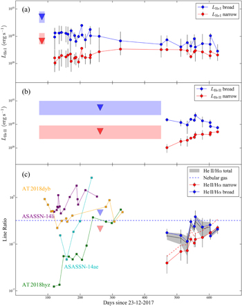
Figure 10. Evolution of (a) He i luminosity, (b) He ii luminosity, and (c) He ii/Hα ratio for the broad (blue points) and narrow (red points) components of the lines. Upper limits are given when the line is not detected (S/N < 2). The median value of upper limits is labeled as downward-pointing triangles, with the range shown as a shaded region. The x-axis is in days since the optical outburst (2017 December 23). In panel (c), the blue dashed line shows He ii/Hα ≃ 0.32 expected for fully ionized gas with solar helium abundance (Hung et al. 2017). The gray curve shows the total He ii/Hα ratio obtained by directly adding the flux of the narrow and broad components, while the gray shaded region marks the 1 σ (16% to 84%) confidence range from our MCMC fitting. The red dashed line gives the narrow He ii/Hα ratio after subtracting the original narrow Hα flux before the optical outburst (Boller et al. 2003). We also plot the line ratios obtained for a few well-known TDEs (squares): ASASSN-14li (purple) and ASASSN-14ae (cyan) from Hung et al. (2017), at 110 days after discovery, and AT 2018dyb (orange) and AT 2018hyz (green) from Charalampopoulos et al. (2022), at 110 days from the peak of their light curves.
Download figure:
Standard image High-resolution imageThe two kinematic components of He i and He ii follow a notably different evolutionary trend: whereas the narrow component rises in strength over time, leveling off to a broad maximum and then possibly turning over in the case of He i, the broad component monotonically decreases with time. He ii is commonly found in TDEs (e.g., Gezari et al. 2012; Hung et al. 2017), many early in their evolution (e.g., ASASSN-14li and AT 2018dyb). However, in none of them does He ii emerge as late as in 1ES 1927+654 (Charalampopoulos et al. 2022). It is also interesting to notice that the He ii/Hα flux ratio behaves very differently among different objects (Figure 10(c)). In general, the ratio is determined first by the temperature of the medium (recombination efficiency) and second by the abundance ratio between He+2 and H+. The median value of He ii/Hα is ∼0.2 (both narrow and broad components combined; Figure 10(c)), somewhat lower than expected for typical fully ionized nebular gas with solar helium abundance (Y⊙ = 0.2485; Serenelli & Basu 2010), for which He ii/Hα ≃ 0.32 (Hung et al. 2017). The lower value of narrow He ii/Hα likely can be attributed to the contamination of Hα emission by the narrow-line region clouds already present prior to the optical outburst. After subtracting the original Hα flux, the "post-outburst" He ii/Hα increased significantly (red dashed line; Figure 10(c)) and finally reached the value for fully ionized He (blue dashed line). This suggests that the photoionized outflowing clouds also decreased in density, in the same manner as the Keplerian bound component, thereby elevating the abundance ratio between He+2 and H+ at late times (see also the discussion in Section 5.2).
4.6. Black Hole Mass Estimates
We have at our disposal several methods to estimate the mass of the BH in 1ES 1927+654. The availability of multiple epochs of optical spectroscopy in principle may allow us to perform RM (Blandford & McKee 1982) to determine the BH mass (e.g., Peterson et al. 2004). However, the observations are too sparsely sampled to yield a robust measurement of the lag between the broad emission-line and continuum light curves, which, in any case, is dominated by an exponential (t−5/3) decline. Instead, we estimate the virial BH mass from the single-epoch spectra, using the broad component of the Balmer lines. Ho & Kim (2015) provide Hβ-based virial mass estimators separately for classical and pseudobulges. In light of the properties of the host galaxy discussed in Section 3.2, we adopt the zero-point appropriate for pseudobulges. The highest-resolution spectrum taken on 2001 June 16 yields  , which is consistent with the value of MBH ≃ 1.9 × 10⁷
M⊙ reported by Trakhtenbrot et al. (2019). However, the full spectral series analyzed in Section 3.3 yields masses that span more than an order of magnitude, from MBH = 1.21 × 10⁷
M⊙ to 32.6 × 10⁷
M⊙ (Figure 11). The Hα-based method of Greene & Ho (2005a) produces a similarly large range of MBH = 0.98 × 10⁷
M⊙ to 26.3 × 10⁷
M⊙, with a median value 7.51 × 10⁷
M⊙. The greatest discrepancy between the two tracers occurs at t ≈ 150–250 days, owing to the large differences between the widths of the two lines during this period (Figure 8(b)). The rapid changes in MBH are clearly unphysical, reflecting the dynamic evolution of the BLR that is not yet virialized (Section 5.2).
, which is consistent with the value of MBH ≃ 1.9 × 10⁷
M⊙ reported by Trakhtenbrot et al. (2019). However, the full spectral series analyzed in Section 3.3 yields masses that span more than an order of magnitude, from MBH = 1.21 × 10⁷
M⊙ to 32.6 × 10⁷
M⊙ (Figure 11). The Hα-based method of Greene & Ho (2005a) produces a similarly large range of MBH = 0.98 × 10⁷
M⊙ to 26.3 × 10⁷
M⊙, with a median value 7.51 × 10⁷
M⊙. The greatest discrepancy between the two tracers occurs at t ≈ 150–250 days, owing to the large differences between the widths of the two lines during this period (Figure 8(b)). The rapid changes in MBH are clearly unphysical, reflecting the dynamic evolution of the BLR that is not yet virialized (Section 5.2).

Figure 11. BH mass (MBH) estimates for 1ES 1927+654. The x-axis is in days since the optical outburst (2017 December 23). The red points show the virial MBH estimated from broad Hα (Greene & Ho 2005a), while the blue points correspond to values based on broad Hβ (Ho & Kim 2015), assuming a virial factor appropriate for pseudobulges (Section 3.2). The large black point represents MBH from the Hβ profile fit of Trakhtenbrot et al. (2019), which is consistent with our results. The three colored horizontal lines and their corresponding shaded regions denote the mass and 1 σ confidence interval estimate from different scaling relations: MBH − Mbulge correlation (Kormendy & Ho 2013;  black), MBH − M* correlation (Greene et al. 2020;
  orange), and MBH − σ* correlation (Saglia et al. 2016;
  cyan).
Download figure:
Standard image High-resolution imageAbsent a trustworthy BH mass based on the broad emission lines, we turn to the properties of the host galaxies for alternatives. The BH mass can be estimated from the MBH − σ* relation (Gebhardt et al. 2000; Ferrarese & Merritt 2000). Since no stellar velocity dispersion is available for the bulge of 1ES 1927+654, we assume σg
≃ σ*, which has been shown to be approximately valid for a large variety of AGNs (e.g., Nelson & Whittle 1996; Greene & Ho 2005b; Ho 2009b; Kong & Ho 2018), where σg
is the velocity dispersion of the ionized gas derived from the narrow forbidden emission lines. Using the three spectra with the highest spectral resolution taken on 2018 March 6–9, we find, after correction for instrumental resolution, FWHM = 217.2 ± 44.1 km s−1 for the [O iii] λ5007 line, or σg
= 92.2 ± 18.7 km s−1. From the MBH − σ* relation for pseudobulges of Saglia et al. (2016),  (cyan dashed line and shaded region in Figure 11). As a cross-check, we also estimate the BH mass from the stellar mass of the bulge. The MBH–Mbulge relation given by Kormendy & Ho (2013) only pertains to elliptical galaxies and classical bulges. We derive the MBH − Mbulge relation for pseudobulges using the sample presented in Kormendy & Ho (2013), fixing the slope to that of classical bulges (1.17) given by Kormendy & Ho, and solving for the zero-point and intrinsic scatter. The relation for pseudobulges is
  , which has an intrinsic scatter of 0.33 dex. From the image decomposition described in Section 2.3, 1ES 1927+654 has B/T ≃ 0.44 in the Ks
band, which, in combination with a rest-frame color of (B − V)0 = 0.42 mag (Section 3.2), results in M/LK
= 0.32 (0.05 dex scatter; Kormendy & Ho 2013),
, which has an intrinsic scatter of 0.33 dex. From the image decomposition described in Section 2.3, 1ES 1927+654 has B/T ≃ 0.44 in the Ks
band, which, in combination with a rest-frame color of (B − V)0 = 0.42 mag (Section 3.2), results in M/LK
= 0.32 (0.05 dex scatter; Kormendy & Ho 2013),  , and hence
  (black dashed line and shaded region in Figure 11). As a final consistency check, the total stellar mass of
  (Section 3.2) implies
  (orange dashed line and shaded region in Figure 11) according to the MBH − M* relation of late-type galaxies from Greene et al. (2020).
In summary, as illustrated in Figure 11, the BH mass estimated using traditional single-epoch virial estimators changes with time and significantly exceeds (by a factor of ∼10) the masses derived from three independent methods based on the properties of the host galaxy. A mass as large as MBH ≈ 107
M⊙ would also be highly unexpected for the relatively low stellar mass of the host galaxy ( ). We suspect that the rapidly evolving BLR of the changing-look event in 1ES 1927+654 is not yet virialized, and therefore its broad emission lines are not suitable for estimating the BH mass. In the following, we adopt
  , based on the MBH − Mbulge relation, since it has the smallest scatter.
5. Discussion
5.1. Witnessing the Transformation of a True Type 2 into a Type 1 AGN
The origin of the BLR in quasars and AGNs remains elusive after decades of research. The broad-line emission may arise from a multiphase medium in which material can condense into clouds through thermal instability (Krolik et al. 1981). Photoionization calculations suggest that, for a specific emission line, the clouds that have the maximum reprocessing efficiency only span a narrow range of density and distance from the central AGN ("locally optimally emitting clouds"; Baldwin et al. 1995). However, clouds cannot survive destruction by Rayleigh–Taylor and Kelvin–Helmholtz instabilities (e.g., Proga & Waters 2015). Confinement by the pressure of an external magnetic field may be necessary (Rees et al. 1989), or perhaps by the pressure gradient developed on the photoionized surface layer of the gas due to the incident radiation force (Baskin et al. 2014; Netzer 2020).
Prior to the optical outburst, 1ES 1927+654 was considered to be a "true" type 2 AGN, on account of its rapid spectral variability and absence of obscuration in the X-rays (Boller et al. 2003), as well as the failure to detect hidden broad emission lines from either optical spectropolarimetry or near-IR spectroscopy (Tran et al. 2011). Thus, 1ES 1927+654 joined the ranks of a small subset of type 2 AGNs suspected to lack a BLR intrinsically (e.g., Tran 2001, 2003; Panessa & Bassani 2002). The intrinsic absence of broad lines is most commonly associated with AGNs of very low accretion rate (Ho 2008), as a consequence of a luminosity limit below which either a BLR cannot survive because its compact size exceeds the maximum allowed velocity (Laor 2003) or there is insufficient column density produced by a radiation-driven wind to sustain a BLR (Elitzur & Ho 2009; Elitzur et al. 2014). However, the BLR can also vanish in a minority of highly accreting AGNs (e.g., Ho et al. 2012; Miniutti et al. 2013), on account of factors (e.g., detailed radial distribution of a radiation-driven wind and radiation efficiency) other than the luminosity that can affect the final BLR column density (Elitzur & Netzer 2016).
Tran et al. (2011) suggested that 1ES 1927+654 might be powered by a highly sub-Eddington ( ), advection-dominated accretion flow. The low accretion luminosity would lead to a very compact BLR, if it were to obey the RBLR − L relation, whose broad lines would be too broad and/or too faint to be detected. NGC 3147 might serve as a possible analog (Bianchi et al. 2019). However, 1ES 1927+654 was bright in the X-rays even before the optical outburst. The 2011 XMM-Newton observation by Gallo et al. (2013) indicated L2–10 keV = 2.4 × 1042 erg s−1, which, with the luminosity-dependent X-ray bolometric correction of Duras et al. (2020), yields a bolometric luminosity of Lbol ≃ 11.5 L2–10 keV = 2.7 ×1043 erg s−1. Assuming MBH = 1.38 × 10⁶
M⊙ (Section 4.6), the corresponding Eddington ratio is λE ≡ Lbol/LE = 0.16, with the Eddington luminosity LE = 1.26 × 1038(MBH/M⊙). If we consider the λE-dependent bolometric correction of Vasudevan & Fabian (2009), Lbol ≃ 70 L2–10 keV = 1.7 × 1044 erg s−1, and λE = 0.97. In either case, it appears unlikely that 1ES 1927+654 was ever faint enough to qualify as advection dominated. Instead, we suggest that the BLR was intrinsically absent before the optical outburst, possibly due to the low column density of the clouds launched by a radiation-driven disk wind. In the disk-wind scenario of Elitzur & Netzer (2016), the minimal bolometric luminosity to ensure the appearance of broad lines must satisfy
), advection-dominated accretion flow. The low accretion luminosity would lead to a very compact BLR, if it were to obey the RBLR − L relation, whose broad lines would be too broad and/or too faint to be detected. NGC 3147 might serve as a possible analog (Bianchi et al. 2019). However, 1ES 1927+654 was bright in the X-rays even before the optical outburst. The 2011 XMM-Newton observation by Gallo et al. (2013) indicated L2–10 keV = 2.4 × 1042 erg s−1, which, with the luminosity-dependent X-ray bolometric correction of Duras et al. (2020), yields a bolometric luminosity of Lbol ≃ 11.5 L2–10 keV = 2.7 ×1043 erg s−1. Assuming MBH = 1.38 × 10⁶
M⊙ (Section 4.6), the corresponding Eddington ratio is λE ≡ Lbol/LE = 0.16, with the Eddington luminosity LE = 1.26 × 1038(MBH/M⊙). If we consider the λE-dependent bolometric correction of Vasudevan & Fabian (2009), Lbol ≃ 70 L2–10 keV = 1.7 × 1044 erg s−1, and λE = 0.97. In either case, it appears unlikely that 1ES 1927+654 was ever faint enough to qualify as advection dominated. Instead, we suggest that the BLR was intrinsically absent before the optical outburst, possibly due to the low column density of the clouds launched by a radiation-driven disk wind. In the disk-wind scenario of Elitzur & Netzer (2016), the minimal bolometric luminosity to ensure the appearance of broad lines must satisfy  . For 1ES 1927+654, this threshold is
  , which, depending on the assumed X-ray bolometric correction, is comparable to or significantly higher than the pre-outburst bolometric luminosity. This may explain why 1ES 1927+654 originally lacked broad lines. The relatively high spin of the BH in 1ES 1927+654 (a* ≈ 0.8, as inferred from broadband SED fitting; Li et al. 2022) may be an additional contributing factor, as the likelihood of a source to be a true type 2 AGN significantly increases with increasing radiation efficiency (Elitzur & Netzer 2016). After the outburst, the optical luminosity of 1ES 1927+654 reached L5100 = 2.30 × 1043 erg s−1, or λE ≈ 1.3 for Lbol = 10 L5100 (Richards et al. 2006). The X-ray luminosity also increased 10-fold (Ricci et al. 2020). During the changing-look event, 1ES 1927+654 lay comfortably above the threshold for BLR formation (Elitzur & Netzer 2016) and formally would be considered super-Eddington, consistent with its very steep X-ray power-law spectrum (Γ ≈ 3; Ricci et al. 2021), which is usually associated with super-Eddington AGNs (e.g., Trakhtenbrot et al. 2017; Ricci et al. 2018).
At the same time, 1ES 1927+65 displays some striking differences compared to ordinary AGNs accreting at or near the Eddington limit. Perhaps the most suitable comparison are the narrow-line Seyfert 1 galaxies (Osterbrock & Pogge 1985), a subclass of type 1 AGNs characterized by narrow Hβ lines (FWHM ≲ 2000 km s−1) and strong Fe ii emission. These properties are a consequence of their relatively low BH masses (MBH ≈ 106–107
M⊙) and high Eddington ratios (Boroson 2002; Shen & Ho 2014). By contrast, 1ES 1927+65, notwithstanding its modest BH mass (MBH ≈ 106
M⊙) and high Eddington ratio (λE ≳ 1), exhibits broad Hβ emission with line widths that range from FWHM ≈ 4000 to nearly 15,000 km s−1. This strongly suggests, as we already argued in connection with the unreasonable virial BH masses obtained in Section 4.6, that the line-emitting region has yet to reach virialization. Another notable distinction lies in the exceptional weakness of Fe ii emission found in the source. The ratio
15
between the equivalent width of Fe ii and Hβ,  , is much less than the value of RFe II ≈ 1 expected for AGNs with λE > 1 (Boroson & Green 1992; Boroson 2002; Dong et al. 2011; Shen & Ho 2014). Boroson (2002) argued that at high Eddington ratios the presence of a soft X-ray excess would produce a large zone of warm, partially ionized, Fe ii-emitting gas. And yet, 1ES 1927+654 emits conspicuously strong soft X-ray emission (Ricci et al. 2021), in strong conflict with its low RFe II.
Interestingly, Fe ii emission also appears to be weak in TDEs reported in other AGNs suspected to be experiencing super-Eddington accretion (e.g., AT 2018dyb; Leloudas et al. 2019). Shields et al. (2010) argue that the strength of Fe ii emission in AGNs is driven not primarily by λE but instead by gas-phase iron abundance. This argument is buttressed by the recent photoionization calculations of Panda (2021), who find that iron must be overabundant to reproduce correctly the observed values of RFe II. If, as we contend (Section 5.2), the BLR clouds in 1ES 1927+65 arose from the condensation of a wind that emanates from an accretion disk freshly created from the debris of a TDE, we naturally expect the material to bear the chemical imprint of the tidally disrupted star, which, in turn, should reflect the metallicity of the overall stellar population of the surrounding galaxy. With a total stellar mass akin to that of the Large Magellanic Cloud (Section 3.2), 1ES 1927+65, too, should have a stellar metallicity of ∼1/2 solar (Choudhury et al. 2016), which is substantially lower than the supersolar values normally inferred for the BLR (e.g., Hamann & Ferland 1999; Jiang et al. 2007). The low metallicity of the clouds might naturally explain the nondetection of typical UV emission lines (e.g., Mg ii) in the Hubble Space Telescope (HST) spectrum taken ∼250 days after the outburst (Trakhtenbrot et al. 2019). Meanwhile, the absence of resonance metal lines (e.g., C iv, C iii]) could reflect the temporary low ionization, which was argued to be the culprit for the lack of He ii then (Section 4.5).
5.2. Physical Picture for the Formation of the BLR
The sudden appearance and rapid secular evolution of the BLR in the changing-look event in 1ES 1927+654 offer us insights that, although not necessarily applicable to typical AGNs, nevertheless may help to elucidate the physical processes associated with the formation of broad emission lines. From the evidence summarized in Section 4, we have shown that (1) broad Hα and Hβ were not detected until t ≈ 100 days after the optical continuum reached its maximum, and (Hα/Hβ)b increased with time; (2) He i was detected at t ≈ 150 days, while it took ∼450 days for He ii to appear; (3) both the continuum luminosity (L5100 ∝ t−5/3) and the FWHM of the broad Balmer lines decreased with time, plausibly suggesting that the changing-look event originated from a TDE (Trakhtenbrot et al. 2019; Ricci et al. 2020, 2021); and (4) the BLR clouds are not virialized, but their velocity shifts are consistent with motions on an eccentric (e ≈ 0.6) Keplerian orbit.
We propose that during the changing-look event in 1ES 1927+654 we witnessed the formation of a BLR. Before the outburst, the host galaxy was highly active but intrinsically lacked broad emission lines because its radiation-driven disk wind launched material with insufficient column density (Section 5.1). The BLR was not formed until the overall luminosity increased above a critical value (Elitzur & Netzer 2016), which was triggered by the TDE. The picture of BLR formation we have in mind has many similarities to the model of Guillochon et al. (2014), who used hydrodynamical simulations to investigate the dynamical evolution of the debris stream formed from the tidal disruption of a main-sequence star by a supermassive BH. According to that work, the debris stream is confined by self-gravity in the two directions perpendicular to the original direction of the star, forming a transient accretion disk that spreads both inward and outward from the pericenter. The authors suggest that the debris stream has a negligible surface area and thus does not contribute significantly to the broad-line emission. Instead, the broad lines are produced by the clouds in the region above and below the forming accretion disk. The model of Guillochon et al. (2014) can reproduce well our observations, and we use it to divide the formation and evolution of the BLR in 1ES 1927+654 into four stages, 16 as schematically sketched in Figure 12:
- 1.Stage 1: Around 2017 December, an optical outburst occurred as a result of a sudden increase of the BH accretion rate induced by the tidal disruption of a star. Debris from the disrupted star formed a temporary accretion disk, which spread both inward and outward (Guillochon et al. 2014). The inward-moving accretion flow collided with the preexisting accretion disk (top left panel), efficiently removing angular momentum and subsequently enhancing the BH accretion rate (Chan et al. 2019). The enhanced accretion rate depleted the inner disk, which led to the disappearance of the X-ray corona (Ricci et al. 2020). Meanwhile, the accretion flow that traveled outward moved on an eccentric Keplerian orbit (top left panel). The orbit, described in detail in Section 4.2, is eccentric (e ≃ 0.6), and its orbital plane has an inclination angle of ∼ 80° with respect to our LOS. The BLR clouds formed above and below the outer region of the eccentric accretion disk, via mechanisms such as condensation from a warm, radiation-pressure-driven disk wind (e.g., Elvis 2017). Adequate column density (>5 × 1021 cm−2; Netzer 2013) was available after the optical outburst from the increase in accretion rate (Elitzur & Netzer 2016; see also discussion in Section 5.1), allowing BLR clouds to form owing to thermal instability in the radiatively heated and cooled medium (Krolik et al. 1981). For a typical AGN environment, the cloud formation timescale is ∼50 days according to radiative hydrodynamical simulations of Proga & Waters (2015), while the acceleration timescale is ∼20 days to reach the local sound speed. These timescales are somewhat shorter than the observed ∼100-day lag between the emergence of the broad lines and the optical outburst, perhaps due to the lower cooling efficiency induced by the low-metallicity environment of the host galaxy (Section 5.1). Once formed, most of the clouds retain the original kinematics, which follow a Keplerian orbit that initially moves toward the LOS. 17 The newly formed BLR clouds produce blueshifted, broad emission lines, as shown in the first row of Figure 7.
- 2.Stage 2: From 100 to 150 days after the outburst, new BLR clouds continued to form, such that the broad-line luminosity increased without an accompanying increase in the continuum. As the size of the accretion disk and the BLR expanded, the width of the broad Balmer lines dropped quickly (Figure 8(b)). Meanwhile, the gas number density (nH) also decreased (Guillochon et al. 2014), leading to the emergence of He i. The ionization potential for He i (24.6 eV) being larger than that of H i (13.6 eV), the strength of the He i λ5877 recombination line should be proportional to the ionization fraction when He i is not fully ionized. Considering the balance between photoionization and recombination, the ionization fraction can be estimated as
 , where I(X0) is the incident rate of photons capable of ionizing the lower state (X0) to the higher state (X+), and ne
is the electron number density. We suggest that initially the BLR clouds were too dense (nH ≈ 1012 cm−3) for He i to be ionized. He i appeared only after the clouds became dilute enough (nH ≈ 1010–1011 cm−3; top right panel) for efficient ionization of He i.
, where I(X0) is the incident rate of photons capable of ionizing the lower state (X0) to the higher state (X+), and ne
is the electron number density. We suggest that initially the BLR clouds were too dense (nH ≈ 1012 cm−3) for He i to be ionized. He i appeared only after the clouds became dilute enough (nH ≈ 1010–1011 cm−3; top right panel) for efficient ionization of He i. - 3.Stage 3: From 150 to 250 days, the broad Balmer lines reached their highest intensity as more and more BLR clouds formed. The clouds occupied a wide range of spatial distribution surrounding the BH (bottom right panel). Not only did the gas number density (nH) decrease for the outlying clouds, but the hydrogen ionizing flux [Φ(H)] also dropped for the outward-moving clouds, since Φ(H) ∝ L r−2, such that as the event progressed the BLR clouds covered an increasingly larger space in the ΦH − nH plane. This scenario also explains the line profiles illustrated in the second and third rows of Figure 7: photoionization calculations (e.g., Korista & Goad 2004) indicate that the equivalent width of broad Hβ and Hα responds differently to nH and ΦH, wherein Hα/Hβ increases with decreasing nH and ΦH. The dependence of density on galactocentric distance (Guillochon et al. 2014) naturally predicts that the strength of broad Hβ and Hα should vary with location along the elliptical orbit, providing a natural explanation for the observed variations in line profile and line ratio.
- 4.Stage 4: Beyond ∼250 days, the high accretion rate of the BH has consumed most of the material (bottom left panel), resulting in a decrease of both the continuum and broad-line luminosity. Broad Hβ and Hα began to fade systematically, and their profiles exhibited a symmetric, redshifted core because the lines were generated mostly by the outer clouds (fourth row of Figure 7). The late emergence of He ii λ4686 can be explained qualitatively in the same manner as He i during stage 2. With an ionization potential of 54 eV, He ii is ionized significantly at this stage—indeed, almost fully ionized by the last epoch (Figure 10(c))—because the inner clouds were rarefied to even lower density.
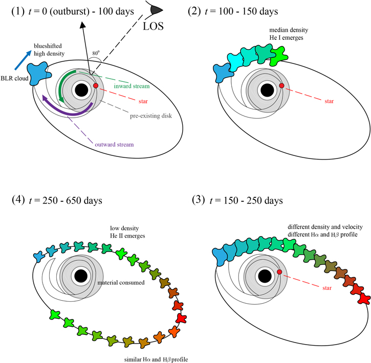
Figure 12. Cartoon showing our proposed scenario for the formation and dynamical evolution of the BLR in the changing-look AGN 1ES 1927+654. Each colored cloud represents a collection of broad-line emitters that has similar location, radial velocity (blue for clouds moving toward our LOS, red for clouds moving away), and density (larger cloud size indicates higher density). We schematically divide the evolution of the event into four successive stages. Stage (1): at t = 0 (outburst) to 100 days, a star (red circle) is tidally disrupted by the supermassive BH, forming a temporary accretion disk. The disk spreads both inward (green arrow) and outward (purple arrow). The temporary, inward-moving accretion flow collides with the preexisting accretion disk, while the material traveling outward moves on an eccentric Keplerian orbit (the outer ellipse). During this phase, BLR clouds can form above and below the elliptical accretion disk (with eccentricity e ≈ 0.6; Section 4.2). The clouds initially have a nonzero radial velocity with respect to the observer (blue cloud). Stage (2): t ≈ 100–150 days after the outburst, the outward-moving clouds have reached densities and an ionization level favorable for the production of He i. Stage (3): at t ≈ 150–250 days, the clouds have both positive and negative radial velocity with respect to the observer, occupy an even larger range in density and ionization, and produce different and asymmetric Hα and Hβ profiles. Stage (4): by t ≈ 250–650 days, the high accretion rate of the BH has consumed most of the material, resulting in a decrease of both the continuum and broad-line luminosity. Meanwhile, the low density of the inner clouds allows He ii to be excited, whose emergence coincides with the presence of weak, redshifted broad Hα emission.
Download figure:
Standard image High-resolution imageThe above physical model offers useful constraints on the lifetime of the clouds in 1ES 1927+654. Clouds newly formed in a radiative environment cannot be sustained against destruction by Rayleigh–Taylor and Kelvin–Helmholtz instabilities. According to the hydrodynamical simulations of Proga & Waters (2015), isobaric clouds can dissolve as quickly as tlife ≈ 10 days, although denser clouds (nH ≥ 1012 cm−3), with their sufficiently large cooling rate, potentially can be nonisobaric and stabilized by conduction (Waters & Proga 2019). During Stage 3, the leading clouds evolve quickly, as evidenced by the notable differences of ΔV, FWHM, and S between broad Hα and Hβ (Figure 8). After ∼250 days, however, the differences disappear, while the line luminosities quickly drop (Figure 6). If we posit that these secular changes are induced by the fragmentation of the leading clouds, we can estimate tlife ≈ 150 days. Once fragmented, the clouds would span more evenly in space, possibly explaining the FWHM "echo" in Figure 8(b).
Scepi et al. (2021), followed by Laha et al. (2022), suggest the alternative scenario that the changing-look event in 1ES 1927+654 can arise from a change in the accretion rate and an inversion of magnetic flux in a magnetically arrested disk. In this picture, the peculiar optical and X-ray light curves result from an inward-leading advection event that brings magnetic flux of the opposite polarity. This model, however, gives no predictions for the broad emission lines after the outburst event, and therefore no direct comparison can be made based on our spectroscopic analysis. These authors attribute the nondetection of broad lines before the outburst to a low AGN power, which, however, is inconsistent with the high accretion rate we deduced for 1ES (Section 5.1).
5.3. Comparison with Other TDEs
The evidence assembled in this study suggests that the BLR clouds of 1ES 1927+654 condensed from a wind radiatively driven from a temporary accretion disk created by the TDE. Here we draw some comparisons of this physical model with parallels seen in a few other TDEs. In hydrodynamical simulation of TDE debris (Guillochon et al. 2014), the density evolution of the clouds is directly linked to their dynamical motion. In the physical scenario offered in Section 5.2, He ii λ4686 emerges when the clouds have evolved to sufficiently low density to allow efficient photoionization of helium. Interestingly, the above scenario of He ii production implies that if the clouds initially were not fully ionized (below the blue dashed line in Figure 10(c)), the He ii/Hα ratio would gradually increase with decreasing cloud density (see examples also in Charalampopoulos et al. 2022). TDEs that exhibit large He ii/Hα immediately after discovery (e.g., ASASSN-14li and ASASSN-14ae) might have clouds of intrinsically lower density or that are helium-rich (Gezari et al. 2012).
The link between density evolution of the clouds and their dynamical motion offers an explanation as to why in 1ES 1927+654 He ii
λ4686 emerged significantly delayed (by ∼240 days relative to the peak of the Hα emission) compared to the handful of other TDEs that initially had low He ii/Hα. In their detailed spectroscopic analysis of AT 2018hyz, whose Hα and Hβ response relative to the optical continuum closely resembles that of 1ES 1927+654, Short et al. (2020) report that He ii appeared roughly 70 days after the Hα peak, much quicker than the 240-day delay observed for 1ES 1927+654. To understand the difference, we note that the average FWHM of the Hα and Hβ lines in AT 2018hyz is ∼ 12, 000 km s−1, about 1.5 times larger than in 1ES 1927+654 (FWHM ≈ 8000 km s−1). Given the similar BH mass (MBH ≈ 106
M⊙; Short et al. 2020), the broader emission lines of AT 2018hyz imply that its BLR clouds are located at smaller semimajor radii, which have correspondingly shorter dynamical timescales: 

 . If the emergence of He ii is related to the dynamical evolution of the disk, the factor of ∼3 in dynamical timescale for the two TDEs can naturally account for the time difference in relative lag between He ii and Hα (0.3 × 240 ≃ 70 days). A similar argument can be made for the TDE PS18kh (Holoien et al. 2019). Although it has a larger BH mass (MBH ≈ 106.9
M⊙) than 1ES 1927+654, its Hα line is also broader (FWHM = 12,000 km s−1), such that their dynamical timescales end up being roughly comparable:
. If the emergence of He ii is related to the dynamical evolution of the disk, the factor of ∼3 in dynamical timescale for the two TDEs can naturally account for the time difference in relative lag between He ii and Hα (0.3 × 240 ≃ 70 days). A similar argument can be made for the TDE PS18kh (Holoien et al. 2019). Although it has a larger BH mass (MBH ≈ 106.9
M⊙) than 1ES 1927+654, its Hα line is also broader (FWHM = 12,000 km s−1), such that their dynamical timescales end up being roughly comparable:  . This may explain why the time delay for the emergence of He ii is almost identical for both, namely, 250 days for PS18kh (Holoien et al. 2019) versus 240 days for 1ES 1927+654. The two TDEs bear a close resemblance in another intriguing aspect. As in 1ES 1927+654 (see Section 4.4), the Balmer decrement of PS18kh increased over time, from (Hα/Hβ)b
≈ 3 initially to ∼7 at late times (Holoien et al. 2019).
. This may explain why the time delay for the emergence of He ii is almost identical for both, namely, 250 days for PS18kh (Holoien et al. 2019) versus 240 days for 1ES 1927+654. The two TDEs bear a close resemblance in another intriguing aspect. As in 1ES 1927+654 (see Section 4.4), the Balmer decrement of PS18kh increased over time, from (Hα/Hβ)b
≈ 3 initially to ∼7 at late times (Holoien et al. 2019).
The changing-look AGN SDSS J015957.64+003310.5 (LaMassa et al. 2015; Zhang 2021) provides a final interesting case for comparison, for, like 1ES 1927+654, its broad Balmer lines exhibit a long-term radial velocity shift (between 2000 and 2010) that may be interpreted as arising from the orbital motion of BLR clouds. With MBH ≈ 106 M⊙ and HαFWHM ≈ 6000 km s−1 (Zhang et al. 2019), the dynamical timescale of SDSS J015957.64+003310.5 is close to twice that of 1ES 1927+654, or ∼7 yr. This is roughly comparable to the 10 yr timescale over which velocity changes were detected. SDSS J015957.64+003310.5 shares another important similarity with 1ES 1927+654 in that its broad Hβ line grossly overestimates by ∼2 orders of magnitude the BH mass predicted by the MBH − σ* relation.
But not all the characteristics of 1ES 1927+654 are reproduced in other TDEs. For example, the broad Hα and Hβ of AT 2018hyz showed no evidence of velocity shift, but instead were asymmetric and double-peaked during the first 100 days (Short et al. 2020). Such double-peaked Balmer lines are found in TDEs (e.g., PTF09djl; Arcavi et al. 2014) whose profiles can be fit well with a relativistic, elliptical accretion disk model (Liu et al. 2017). If this model applies to AT 2018hyz, it implies that its broad, double-peaked Balmer lines are produced in low-density, optically thin material just above the disk (Gomez et al. 2020), conditions perhaps unfavorable for cloud condensation that would result in detectable changes in velocity or Balmer decrement. By contrast, the broad Hα and Hβ lines of 1ES 1927+654 remained quite symmetric throughout our observations (S > 0.7; Figure 6(b)), decidedly distinct from the highly asymmetric or double-peaked broad profiles expected from a disk. The disk model also has difficulty accounting for the velocity shifts of 1ES 1927+654, which can be modeled by a simple Keplerian orbit (Figure 8(a)).
The above-mentioned differences between 1ES 1927+654 and other TDEs suggests an alternative explanation for the double-peaked Balmer line profile, namely, that it might comprise two kinematic distinct components, a main Keplerian component and an additional outflow component, as commonly invoked in velocity-resolved RM models of type 1 AGNs (Pancoast et al. 2014; Li et al. 2018; Williams et al. 2018). If we were to view the TDE disk from a more face-on orientation, the outflowing broad-line clouds would contribute a blue horn to the original broad profile, but we would see little velocity shift evolution, as in the case of AT 2018hyz. For a more edge-on view, the additional flux would be centered closer to the rest wavelength, and more significant velocity shift evolution would be seen, as in the case of 1ES 1927+654 and ASASSN-18pg (Holoien et al. 2020). Since the two components can have intrinsically different light curves (Figure 6), the disappearance of the second Hα peak of AT 2018hyz (Short et al. 2020) after ∼100 days can be attributed to the decrease of the flux of the outflow component. The two-component BLR model provides an alternative to the reprocessing scenario (Dai et al. 2018) to explain the viewing angle dependence of the observed spectroscopic properties of TDEs (Charalampopoulos et al. 2022).
The roughly t−5/3 decline of both the optical (Figure 4(a)) and UV (Trakhtenbrot et al. 2019) continuum is consistent with the fallback accretion rate of TDEs (Rees 1988). While a similar light curve is expected in the X-rays (Saxton et al. 2021), this is not observed in 1ES 1927+654 (Ricci et al. 2020, 2021). Ricci et al. (2020) argue, based on the evolution of the X-ray hardness, that the X-ray corona might be destroyed around 200 days, after which it gradually gets recreated. Perhaps this event can be linked to the interaction between the preexisting disk and the debris from a tidally disrupted star. In this respect, 1ES 1927+654, already active prior to the outburst, fundamentally differs greatly from other TDEs.
6. Summary
1ES 1927+654, historically a "true" type 2 AGN (Boller et al. 2003; Tran et al. 2011) with relatively high accretion rate, transitioned into a type 1 AGN on 2017 December 23 with the appearance of a blue continuum and broad optical emission lines (Trakhtenbrot et al. 2019). The changing-look event was accompanied by a sharp drop and then rebound in the X-rays ∼200 days after the outburst (Ricci et al. 2020, 2021). The optical continuum light curve and overall evolution of the broad emission lines suggest that the changing-look event was associated with a TDE. In this work, we provide a detailed analysis of the properties of the host galaxy, with the primary aim of securing an independent constraint on the mass of the central BH. To ascertain the host galaxy morphology, bulge type, and stellar mass, we perform 2D image decomposition of optical images acquired with XMM-Newton prior to the outburst, supplemented by SED modeling of optical spectra and broadband (UV, optical, and near-IR) photometry. We study 34 optical spectra covering a period of ∼500 days to conduct a thorough investigation of the spectral evolution of the AGN outburst, to elucidate the origin and characteristics of the BLR.
With a stellar mass of merely  , the host galaxy of 1ES 1927+654 is relatively young (stellar population age ≃ 1 Gyr) and likely hosts a pseudobulge that composes 44% of the total mass. We use these mass measurements and an estimate of the stellar velocity dispersion of the bulge, in conjunction with standard scaling relations between BH mass and host galaxy properties, to bracket the BH mass in the range ∼ (1–5) × 106
M⊙, with a preferred, final adopted value of
, the host galaxy of 1ES 1927+654 is relatively young (stellar population age ≃ 1 Gyr) and likely hosts a pseudobulge that composes 44% of the total mass. We use these mass measurements and an estimate of the stellar velocity dispersion of the bulge, in conjunction with standard scaling relations between BH mass and host galaxy properties, to bracket the BH mass in the range ∼ (1–5) × 106
M⊙, with a preferred, final adopted value of  . At the peak of the AGN outburst, the bolometric luminosity of the BH exceeded the Eddington limit (λE ≃ 1.3).
During the course of the monitoring campaign, 1ES 1927+654 displayed dramatic spectral variability, as follows:
- 1.Contrary to the behavior in the X-rays, the optical continuum luminosity decreased monitonically with time, roughly as t−5/3 as observed in TDEs. The spectral index of the continuum was initially close to that predicted for a standard thin disk (fν ∝ ν+0.33), and then, after an erratic drop around 200 days after the outburst, gradually fell to a value typically found in normal quasars (fν ∝ ν−0.44).
- 2.The broad Balmer lines emerged at ∼100 days, and their flux rose sharply to a prolonged maximum that extended from ∼120 to 230 days. The Balmer decrement of the broad lines increased substantially and systematically from (Hα/Hβ)b ≈ 1 to 5.
- 3.The kinematics of the broad Balmer lines changed in a complex but systematic manner. The radial velocities were initially blueshifted, but they became redshifted by the end of the observation campaign, following a trend with time that can described by an eccentric (e ≈ 0.6) Keplerian orbit. The FWHM of broad Hα and Hβ decreased by a factor ∼2 from the time the lines first appeared to the last epoch of observation. The profiles were roughly symmetric at the beginning and the end of the campaign, but they transitioned to a period of high asymmetry when they were strongest at ∼100–200 days.
- 4.We detected a new component of narrow Balmer emission. Narrow Hα and Hβ systematically increased in strength by as much as a factor of 4 after 200 days, and then gradually declined. By the end of the last epoch they had not yet returned to their pre-outburst level. The light curves for the narrow lines rose and fell more gradually than those of the broad lines.
- 5.Helium lines were detected later than the hydrogen Balmer lines, at ∼150 days for He i λ5877 and ∼450 days for He ii λ4686. The ratio of narrow He ii/Hα increased significantly at late times, until finally reaching the value for fully ionized nebular gas.
The above observational characteristics paint a complex yet consistent physical picture for the changing-look event in 1ES 1927+654. We propose that the debris of a tidally disrupted star formed a temporary accretion disk. The super-Eddington accretion event drove a strong disk wind, which promoted the condensation of clouds whose density and kinematics changed systematically throughout their orbital evolution, as manifested by the appearance of emission lines of varying strength, ionization, relative intensity, velocity width, and asymmetry. An unavoidable consequence of such a dynamically evolving BLR is that the common practice of using the broad lines to derive a virial mass for the central BH is invalid, as evidenced by the time-varying BH masses inferred from broad Hα and Hβ, which appear grossly overestimated compared to the mass estimates based on the host galaxy properties. This study highlights the value of coordinated, long-term spectroscopic monitoring of TDEs and changing-look AGNs, which can serve as an effective laboratory for elucidating the physical processes around the central engine of supermassive BHs.
We thank the anonymous referee for helpful suggestions. This work was supported by the National Science Foundation of China (11721303, 11991052, 12011540375) and the China Manned Space Project (CMS-CSST-2021-A04, CMS-CSST-2021-A06). C.R. acknowledges support from the Fondecyt Iniciacion grant 11190831. B.T. acknowledges support from the European Research Council (ERC) under the European Union's Horizon 2020 research and innovation program (grant agreement 950533) and from the Israel Science Foundation (grant 1849/19). I.A. is a CIFAR Azrieli Global Scholar in the Gravity and the Extreme Universe Program and acknowledges support from that program, from the European Research Council (ERC) under the European Unions Horizon 2020 research and innovation program (grant agreement No. 852097), from the Israel Science Foundation (grant No. 2752/19), from the United States—Israel Binational Science Foundation (BSF), and from the Israeli Council for Higher Education Alon Fellowship.
Software: SAS (v18.0.0; Gabriel et al. 2004), SExtractor (Bertin & Arnouts 1996), GALFIT (Peng et al. 2002, 2010), photutils (Bradley et al. 2019), IRAF (Tody 1986, 1993), lmfit (Newville et al. 2021), emcee (Foreman-Mackey et al. 2013).
Appendix: The Effect of Spectral Resolution on Velocity Shift Measurements
Our interpretation of a rapidly evolving BLR relies on detailed decomposition of the multiepoch spectra. However, the spectra from different instruments deliver a range of spectral resolution, from R ≈ 400 for data taken with FLOYDS 18 to R ≈ 5000 for spectra from DIS. 19 To test the robustness of our results, we generate a series of simulated spectra that resemble the spectral resolution and S/N of the data and repeat the spectral decomposition.
We focus on the two spectral regions most relevant to our analysis, namely, the Hβ region (4430–5200 Å) and the Hα region (6100–7100 Å), and we mimic the conditions for the FLOYDS data set, which has the sparsest sampling (Δλ ≈ 1.7 Å) and lowest spectral resolution (R ≈ 400). For each epoch of the observation, we simulate 100 mock spectra drawn from the S/N distribution, using the best-fit model of the original spectrum as the input. We perform least-squares minimization of the 100 realizations to derive the distribution of the best-fit parameters. Since the average FWHM of the broad Balmer lines ( ∼ 9000 km s−1) is much larger than the lowest spectral resolution (750 km s−1), the output values of the FWHM derived from the mock spectra are, as expected, quite consistent with our measurements. The median differences are small for line width (ΔFWHM/FWHM = 2% ± 19%) and broad Balmer line luminosity (ΔLHα
/LHα
= − 2% ± 14%; ΔLHβ
/LHβ
= − 0.5% ± 18%). The output velocity shift, as illustrated in Figure A1, shows good consistency for broad Hα
 ). The situation is much worse for broad Hβ, which exhibits not only a large scatter but also a systematic bias
  ) because of severe blending with broad He ii, especially when Hβ is weak (S/N < 2). Consequently, when fitting the evolution of ΔV with our Keplerian model (Section 4.2), we only use ΔVHα
.
) because of severe blending with broad He ii, especially when Hβ is weak (S/N < 2). Consequently, when fitting the evolution of ΔV with our Keplerian model (Section 4.2), we only use ΔVHα
.
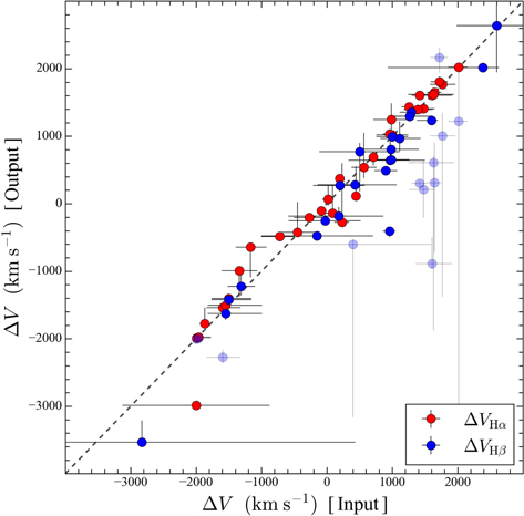
Figure A1. Simulation test on velocity shift (ΔV) measurements for 1ES 1927+654. The x-axis is derived from our MCMC best-fit model (Section 3.3). Each point indicates an individual epoch. The y-axis is derived from fitting simulated spectra; each point represents 100 realizations, where the error bar is calculated from the 16% and 84% values. Weak detections of Hβ (S/N < 2) are labeled by lighter color. The dashed line denotes the one-to-one relation.
Download figure:
Standard image High-resolution image
Footnotes
- 10
XMM-Newton Users Handbook: https://xmm-tools.cosmos.esa.int/external/xmm_user_support/documentation/uhb/omlimits.html.
- 11
Rest-frame wavelength intervals: 3820−3900 Å, 4060−4140 Å, 4300−4380 Å, 4820−4900 Å, 4920−5050 Å, 6500−6620 Å, and 6670−6770 Å.
- 12
The best-fit result with only one SSP left a strong residual on the blue part of the optical spectrum and the XMM-Newton OM UVM2 and UVW1 points, requiring a composite stellar population to achieve a decent fit. Our tests indicate that adding additional SSPs does not improve the fit significantly.
- 13
We tried to fit different values of i and found that i = 80° best describes the data. Lower i (face-on inclination) would result in values of a too small to match the observed ΔV.
- 14
We focus on Hα because it has higher S/N compared to Hβ or He i, and because the tests described in the Appendix indicate that the velocity shifts measured from broad Hα, unlike those from broad Hβ, are robust against the low spectral resolution of some of our data.
- 15
- 16
- 17
As mentioned in Section 4.5, ∼10% of the clouds had outflow kinematics that depart from Keplerian motion.
- 18
- 19