COLOSSUS: A Python Toolkit for Cosmology, Large-scale Structure, and Dark Matter Halos

In Colossus, the cosmology is set globally so that it does not need to be passed to functions. If necessary, the user can store multiple cosmology objects and activate them in turn. For convenience, the user can choose from an extensive list of pre-defined sets of cosmological parameters (Table 1).

Table 1.  Pre-set Cosmologies

ID	rel	H0	${{\rm{\Omega }}}_{{\rm{m}}}$	${{\rm{\Omega }}}_{{\rm{b}}}$	${n}_{{\rm{s}}}$	${\sigma }_{8}$	Reference	Comment
planck18	yes	67.66	0.3111	0.0490	0.9665	0.8102	Planck Coll. (2018), Table 2	Best fit, with BAO (column 6)
planck18-only	yes	67.36	0.3153	0.0493	0.9649	0.8111	Planck Coll. (2018), Table 2	Best fit, Planck only (column 5)
planck15	yes	67.74	0.3089	0.0486	0.9667	0.8159	Planck Coll. (2016), Table 4	Best fit, with external data (column 6)
planck15-only	yes	67.81	0.3080	0.0484	0.9677	0.8149	Planck Coll. (2016), Table 4	Best fit, Planck only (column 2)
planck13	yes	67.77	0.3071	0.0483	0.9611	0.8288	Planck Coll. (2014), Table 5	Best fit, with external data
planck13-only	yes	67.11	0.3175	0.0490	0.9624	0.8344	Planck Coll. (2014), Table 2	Best fit, Planck only
WMAP9	yes	69.32	0.2865	0.0463	0.9608	0.8200	Hinshaw et al. (2013), Table 4	Best fit, combined data
WMAP9-only	yes	69.70	0.2814	0.0464	0.9710	0.8200	Hinshaw et al. (2013), Table 2	Max. likelihood, WMAP only
WMAP9-ML	yes	69.70	0.2821	0.0461	0.9646	0.8170	Hinshaw et al. (2013), Table 2	Max. likelihood, combined data
WMAP7	yes	70.20	0.2743	0.0458	0.9680	0.8160	Komatsu et al. (2011), Table 1	Best fit, with BAO and H0
WMAP7-only	yes	70.30	0.2711	0.0451	0.9660	0.8090	Komatsu et al. (2011), Table 1	Max. likelihood, WMAP only
WMAP7-ML	yes	70.40	0.2715	0.0455	0.9670	0.8100	Komatsu et al. (2011), Table 1	Max. likelihood, with BAO and H0
WMAP5	yes	70.50	0.2732	0.0456	0.9600	0.8120	Komatsu et al. (2009), Table 1	Best fit, with BAO and SNe
WMAP5-only	yes	72.40	0.2495	0.0432	0.9610	0.7870	Komatsu et al. (2009), Table 1	Max. likelihood, WMAP only
WMAP5-ML	yes	70.20	0.2769	0.0459	0.9620	0.8170	Komatsu et al. (2009), Table 1	Max. likelihood, with BAO and SNe
WMAP3	yes	73.50	0.2342	0.0413	0.9510	0.7420	Spergel et al. (2007), Table 5	Best fit, WMAP only
WMAP3-ML	yes	73.20	0.2370	0.0414	0.9540	0.7560	Spergel et al. (2007), Table 2	Max. likelihood, WMAP only
WMAP1	yes	72.00	0.2700	0.0463	0.9900	0.9000	Spergel et al. (2003), Table 7/4	Best fit, WMAP only
WMAP1-ML	yes	68.00	0.3136	0.0497	0.9700	0.9000	Spergel et al. (2003), Table 1/4	Max. likelihood, WMAP only
illustris	no	70.40	0.2726	0.0456	0.9630	0.8090	Vogelsberger et al. (2014)	Cosmology of the Illustris simulation
bolshoi	no	70.00	0.2700	0.0469	0.9500	0.8200	Klypin et al. (2011)	Cosmology of the Bolshoi simulation
multidark-planck	no	67.80	0.3070	0.0480	0.9600	0.8290	Klypin et al. (2016)	Cosmology of the Multidark-Planck simulations
millennium	no	73.00	0.2500	0.0450	1.0000	0.9000	Springel et al. (2005)	Cosmology of the Millennium simulation
EdS	no	70.00	1.0000	0.0000	1.0000	0.8200	⋯	Einstein-de Sitter cosmology

Note. All cosmologies listed are flat ΛCDM cosmologies, i.e., they have no curvature and $w=-1$ (or no dark energy in the case of an Einstein-de Sitter cosmology). The "rel" field indicates whether relativistic species (neutrinos and radiation) are included. By default, they are included, except for the cosmologies of numerical simulations that do not explicitly follow relativistic species. The cosmology of the IllustrisTNG simulation suite is equivalent to the "planck15" cosmology (Pillepich et al. 2018).

Download table as:  ASCIITypeset image

For many of its functions, the cosmology module relies on the interpolation of lookup tables to speed up the evaluation. These tables are computed on demand, i.e., when a function is first evaluated for a given cosmology. The number of bins in the tables was adjusted to obtain a particular accuracy. The interpolation uses cubic splines that are also used to invert the functions (e.g., give z(t) rather than t(z)) and evaluate derivatives (e.g., dz/dt or dt/dz). However, no guarantee is given on the accuracy of the derivatives, particularly for higher-order derivatives.

Table 2 gives an overview of the accuracy and range of validity of key functions in the cosmology module. The quoted accuracy refers to the default parameters, but can be modified by the user in a number of ways. First, interpolation can be turned off altogether, though at a significant performance penalty. Second, the accuracy of many computations (such as numerical integrations) can be altered from the default settings. Finally, the user can change the binning scheme of the lookup tables, though this is generally not recommended.

Table 2.  Accuracy and Range of Validity of Key Functions in the Cosmology Module

Function	Dependent Funcs. (Incomplete List)	Section	Rangea	Comput. acc.b	Interp. acc.b	Inverse	Derivs.c
Hubble parameter E(z)	Densities, times	2.3	$-0.995\lt z\lt 200$	Mach. precision	⋯	no	⋯
Age of the universe	⋯	2.3	$-0.995\lt z\lt 200$	10−8	$6\times {10}^{-5}$	yes	1st, 2nd
Comoving distance	Angular diameter/luminosity dist.	2.3	$-0.995\lt z\lt 200$	10−8	⋯	yes	1st, 2nd
Angular diameter dist.	⋯	2.3	$0\lt z\lt 200$	10−8	$9\times {10}^{-5}$	no	1st, 2nd
Luminosity distance	⋯	2.3	$0\lt z\lt 200$	10−8	$6\times {10}^{-4}$	yes	1st, 2nd
Linear growth factor	Power spectrum, variance, etc	2.4	$-0.995\lt z\lt 200$	10−6 (low z)d	$2\times {10}^{-4}$	yes	1st, 2nd
Linear power spectrum	Variance, correlation function	2.5	${10}^{-20}\lt k\lt {10}^{20}$	5% (EH98)	$3\times {10}^{-4}$	yes	1st
Variance	Peak height, nonlinear mass	2.6	${10}^{-12}\lt R\lt {10}^{3}$	$3\times {10}^{-3}$ e	$5\times {10}^{-3}$	yes	1st
Correlation function	2-halo term	2.7	${10}^{-3}\lt R\lt 5\times {10}^{2}$	10−5 e	10−2	no	1st

Notes.

^aMany of the functions listed can be evaluated outside the given redshift range but have not been tested in those regimes. The ranges are given in the native units of the cosmology module, i.e., $\mathrm{Mpc}\,{h}^{-1}$ for distances and radii and $h\,{\mathrm{Mpc}}^{-1}$ for wavenumbers. A number of functions (the power spectrum, variance, and correlation function) depend on redshift through the linear growth factor, which thus defines the redshift range over which they can be reliably computed. ^bThe table gives two different indicators of accuracy, namely the maximum error to which a quantity is computed (for example, in an integration), and the additional error due to interpolation. The latter can be avoided by switching interpolation off, though at a (sometimes steep) performance penalty. The interpolation error quoted here is the maximum error found at any redshift in a number of representative cosmologies. ^cSome functions can return their first derivative, and some functions return even higher orders. Note, however, that the accuracy of those derivatives is not guaranteed and likely to get worse at higher orders due to interpolation errors. In particular, cubic splines are prone to ringing that has virtually no effect on the solution but affects the higher derivatives of the spline. ^dThe linear growth factor is computed to an integration accuracy of 10⁻⁶ at low redshift, but at high z relies on the fitting function of Gnedin et al. (2011), for which no estimate of the accuracy is given. ^eThe accuracy of the variance and correlation function refers to the accuracy of the integration and does not include the (generally much larger) inaccuracies due to the underlying approximation of the power spectrum (see Sections 2.6 and 2.7 for estimates of those errors).

Download table as:  ASCIITypeset image

Constructing all cosmological interpolation tables takes about 1.7 s on a typical machine (2015 MacBook Pro, Python 3.5). This time is dominated by the correlation function without which the calculation is reduced to about 0.15 s. Importantly, interpolation tables are computed only once: after the first execution, they are stored on disk and loaded on demand. To ensure that only matching tables are loaded for a given cosmology, all relevant parameters are expressed as a string and converted to a unique hash identifier using the md5 algorithm. The tables are discarded when cosmological parameters are changed.

Cosmology objects are initiated from a set of cosmological parameters and settings, including the Hubble constant H₀ (often denoted $h\equiv {H}_{0}/(100\,\mathrm{km}\,{{\rm{s}}}^{-1}\,{\mathrm{Mpc}}^{-1})$), the primordial power spectrum index ${n}_{{\rm{s}}}$, the power spectrum normalization ${\sigma }_{8}$, and the densities of certain species. The Colossus cosmology includes the densities of matter (dark matter and baryons), baryons, dark energy, curvature, photons, neutrinos, and the sum of relativistic species (photos and neutrinos), denoted ${\rho }_{{\rm{m}}}$, ${\rho }_{{\rm{b}}}$, ${\rho }_{\mathrm{de}}$, ${\rho }_{{\rm{k}}}$, ${\rho }_{\gamma }$, ${\rho }_{\nu }$, and ${\rho }_{\mathrm{rel}}$, respectively. Their fraction with respect to the critical density, ${\rho }_{{\rm{c}}}$, are denoted ${{\rm{\Omega }}}_{{\rm{m}}}$, ${{\rm{\Omega }}}_{{\rm{b}}}$, ${{\rm{\Omega }}}_{\mathrm{de}}$, ${{\rm{\Omega }}}_{{\rm{k}}}$, ${{\rm{\Omega }}}_{\gamma }$, ${{\rm{\Omega }}}_{\nu }$, and ${{\rm{\Omega }}}_{\mathrm{rel}}$, their values at z = 0 as ${\rho }_{{\rm{m}},0}$ and ${{\rm{\Omega }}}_{{\rm{m}},0}$ and so on. The user can specify whether a flat cosmology is assumed and whether relativistic species should be included. By default, the cosmology does contain relativistic species, namely radiation and neutrinos whose contributions are computed as follows. The density of radiation today follows from the Stefan–Boltzmann law for a blackbody:

$$\begin{eqnarray}&&{\rho }_{\gamma ,0}=4{\sigma }_{\mathrm{SB}}{T}_{\mathrm{CMB},0}^{4},\end{eqnarray} \tag{ 1 }$$

where ${\sigma }_{\mathrm{SB}}$ is the Stefan–Boltzmann constant. Dividing by the critical density and converting to the appropriate units, we find

$$\begin{eqnarray}&&{{\rm{\Omega }}}_{\gamma ,0}=\displaystyle \frac{4.4813\,\times \,{10}^{-7}}{{h}^{2}}{\left(\displaystyle \frac{{T}_{\mathrm{CMB},0}}{K}\right)}^{4}\approx 5.4\,\times \,{10}^{-5},\end{eqnarray} \tag{ 2 }$$

where we have assumed a default CMB temperature of ${T}_{\mathrm{CMB},0}=2.7255\,{\rm{K}}$ (Fixsen 2009) and the "planck15" cosmology (Table 1). The density of neutrinos is

$$\begin{eqnarray}&&{{\rm{\Omega }}}_{\nu ,0}=\displaystyle \frac{7}{8}{\left(\displaystyle \frac{4}{11}\right)}^{4/3}{N}_{\mathrm{eff}}{{\rm{\Omega }}}_{\gamma ,0}\approx 0.69\,{{\rm{\Omega }}}_{\gamma ,0}\approx 3.7\,\times \,{10}^{-5},\end{eqnarray} \tag{ 3 }$$

where the effective number of neutrino species, ${N}_{\mathrm{eff}}=3.046$, accounts for three neutrino species and subtle effects that influence the ratio of the photon and neutrino temperatures (Mangano et al. 2002; de Salas & Pastor 2016; Planck Collaboration et al. 2018). The user can, of course, set different values for ${T}_{\mathrm{CMB},0}$ and ${N}_{\mathrm{eff}}$, but the neutrino mass is currently fixed.

Finally, we need to compute the contributions from curvature and dark energy. If the cosmology is flat, ${{\rm{\Omega }}}_{{\rm{k}},0}=0$ and

$$\begin{eqnarray}&&{{\rm{\Omega }}}_{\mathrm{de},0}=1-{{\rm{\Omega }}}_{{\rm{m}},0}-{{\rm{\Omega }}}_{\gamma ,0}-{{\rm{\Omega }}}_{\nu ,0}.\end{eqnarray} \tag{ 4 }$$

If the user has chosen a non-flat cosmology, ${{\rm{\Omega }}}_{\mathrm{de},0}$ needs to be set and we compute

$$\begin{eqnarray}&&{{\rm{\Omega }}}_{{\rm{k}},0}=1-{{\rm{\Omega }}}_{\mathrm{de},0}-{{\rm{\Omega }}}_{{\rm{m}},0}-{{\rm{\Omega }}}_{\gamma ,0}-{{\rm{\Omega }}}_{\nu ,0}.\end{eqnarray} \tag{ 5 }$$

Dark energy is described by an equation of state parameter $w(z)=P(z)/\rho (z)$, which can be −1 (a cosmological constant resulting in a ΛCDM cosmology), a constant other than −1 (wCDM), linearly varying with redshift according to Chevallier & Polarski (2001),

$$\begin{eqnarray}&&w(z)={w}_{0}+{w}_{{\rm{a}}}\displaystyle \frac{z}{z\,+\,1},\end{eqnarray} \tag{ 6 }$$

or follow an arbitrary function w(z) set by the user.

The scale factor a is defined as usual, a = 1 at z = 0. Many cosmological quantities rely on the Hubble constant as a function of time, normalized to the z = 0 value,

$$\begin{eqnarray}&&E(a)=\sqrt{{{\rm{\Omega }}}_{{\rm{m}},0}{a}^{-3}+{{\rm{\Omega }}}_{{\rm{k}},0}{a}^{-2}+{{\rm{\Omega }}}_{\mathrm{rel},0}{a}^{-4}+f(z){{\rm{\Omega }}}_{\mathrm{de},0}},\end{eqnarray} \tag{ 7 }$$

where f(z) encapsulates any possible evolution of the dark energy equation of state,

$$\begin{eqnarray}&&f(z)=\exp \left(3{\int }_{0}^{\mathrm{ln}(1+z)}[1+w(z^{\prime} )]d\mathrm{ln}(1+z^{\prime} )\right).\end{eqnarray} \tag{ 8 }$$

This expression evaluates to unity for a cosmological constant, to $f(z)={a}^{-3(1+{w}_{0})}$ for $w={w}_{0}$, and to

$$\begin{eqnarray}&&f(z)={a}^{-3(1+{w}_{0}+{w}_{{\rm{a}}})}{e}^{-3{w}_{{\rm{a}}}(1-a)}\end{eqnarray} \tag{ 9 }$$

for $w(z)={w}_{0}+{w}_{{\rm{a}}}(1-a)$ (Chevallier & Polarski 2001; Linder 2003). Colossus always computes E(z) exactly, i.e., without any interpolation. The critical density is evaluated as ${\rho }_{{\rm{c}}}(z)\,={\rho }_{{\rm{c}},0}{E}^{2}(z)$, whereas the other densities (${\rho }_{{\rm{m}}}$, ${\rho }_{{\rm{b}}}$, ${\rho }_{\mathrm{de}}$, ${\rho }_{\gamma }$, ${\rho }_{\nu }$) are computed from their z = 0 values and the redshift scalings implied by Equation (7). A number of quantities depend on integrals of E(z), and these quantities are stored in interpolation tables to avoid repeated evaluation of the integrals. For example, the age of the universe is

$$\begin{eqnarray}&&t(z)=\displaystyle \frac{1}{{H}_{0}}{\int }_{z}^{\infty }\displaystyle \frac{{dz}}{E(z)\times (1+z)}.\end{eqnarray} \tag{ 10 }$$

All times are expressed in units of Gyr in Colossus. The line-of-sight comoving distance to a particular redshift is

$$\begin{eqnarray}&&{d}_{\mathrm{com},\mathrm{los}}(z)=\displaystyle \frac{c}{{H}_{0}}{\int }_{0}^{z}\displaystyle \frac{1}{E(z)},\end{eqnarray} \tag{ 11 }$$

where all distances are expressed in units of comoving $\,{h}^{-1}\,\mathrm{Mpc}$. The distance between two events at the same redshift that are separated by an angle of one radian depends on whether the cosmology is flat or not,

$$\begin{eqnarray}{d}_{\mathrm{com},\mathrm{trans}}(z)=\left\{\begin{array}{ll}\displaystyle \frac{c/{H}_{0}}{\sqrt{{{\rm{\Omega }}}_{{\rm{k}},0}}}\sinh \left(\displaystyle \frac{\sqrt{{{\rm{\Omega }}}_{{\rm{k}},0}}}{c/{H}_{0}}{d}_{\mathrm{com},\mathrm{los}}\right) & \forall \,{{\rm{\Omega }}}_{{\rm{k}},0}\gt 0\\ {d}_{\mathrm{com},\mathrm{los}} & \forall \,{{\rm{\Omega }}}_{{\rm{k}},0}=0\\ \displaystyle \frac{c/{H}_{0}}{\sqrt{-{{\rm{\Omega }}}_{{\rm{k}},0}}}\sin \left(\displaystyle \frac{\sqrt{-{{\rm{\Omega }}}_{{\rm{k}},0}}}{c/{H}_{0}}{d}_{\mathrm{com},\mathrm{los}}\right) & \forall \,{{\rm{\Omega }}}_{{\rm{k}},0}\lt 0\end{array}\right..\end{eqnarray} \tag{ 12 }$$

In Colossus, this distance is referred to as the "transverse comoving distance" (e.g., Hogg 1999), but a number of other terms are used in the literature, e.g., "comoving angular diameter distance" (Dodelson 2003), "comoving coordinate distance" (Mo et al. 2010), or "angular size distance" (Peebles 1993). The latter is not to be confused with the angular diameter distance ${d}_{\mathrm{ang}}={d}_{\mathrm{com},\mathrm{trans}}/(1+z)$ or the luminosity distance ${d}_{\mathrm{lum}}={d}_{\mathrm{com},\mathrm{trans}}(1+z)$.

The Colossus results for densities, distances, and times agree to a few times 10⁻⁴ or better with those computed by astropy, which was itself tested against several other calculators (The Astropy Collaboration et al. 2013). By default, interpolation is used to speed up the evaluations. For this purpose, Colossus computes tables with 50 bins in redshift, equally spaced in $\mathrm{ln}(1+z)$. The resulting interpolation errors are a few times 10⁻⁴ or better in all quantities, at all redshifts, and over a range of representative cosmologies (Table 2).

The final quantity that relies on an integral of E(z) is the linear growth factor, ${D}_{+}(z)$, the time-dependent normalization of the linear fluctuations in the density field. The value of ${D}_{+}$ is influenced by relativistic species at high redshift and by dark energy at low redshift, leading to different possibilities for the normalization of ${D}_{+}$ (e.g., Eisenstein & Hu 1999; Percival 2005). Internally, Colossus computes the growth factor such that ${D}_{+}(a)=a$ at high redshift, as is the case in an Einstein-de Sitter cosmology. By default, the growth factor is renormalized such that ${D}_{+}(z=0)=1$, but the user can request either normalization.

We compute ${D}_{+}$ by splitting the redshift range into multiple segments. At $z\gt 10$, ${D}_{+}$ is approximated using Equation (5) in Gnedin et al. (2011),

$$\begin{eqnarray}\begin{array}{rcl}{D}_{+}(a) & = & a+\displaystyle \frac{2}{3}{a}_{\mathrm{mr}}+\displaystyle \frac{{a}_{\mathrm{mr}}}{2\mathrm{ln}(2)-3}\\ & \times & \left[2\sqrt{1+x}+\left(\displaystyle \frac{2}{3}+x\right)\mathrm{ln}\displaystyle \frac{\sqrt{1+x}-1}{\sqrt{1+x}+1}\right],\end{array}\end{eqnarray} \tag{ 13 }$$

where $x\equiv a/{a}_{\mathrm{mr}}$ and ${a}_{\mathrm{mr}}\equiv {{\rm{\Omega }}}_{\mathrm{rel},0}/{{\rm{\Omega }}}_{{\rm{m}},0}$ is the epoch of matter-radiation equality. If relativistic species are not included in the cosmology, ${D}_{+}(a)=a$ in this redshift regime. The relativistic corrections become very small at low redshift and can be neglected, but dark energy needs to be taken into account instead. The evolution of ${D}_{+}$ is determined by the differential equation

$$\begin{eqnarray}&&{D}_{+}^{{\prime\prime} }+\displaystyle \frac{3}{2a}\left[1-\displaystyle \frac{w(a)}{1+X(a)}\right]{D}_{+}^{{\prime} }-\displaystyle \frac{3X(a)}{2[1+X(a)]{a}^{2}}{D}_{+}=0,\end{eqnarray} \tag{ 14 }$$

where $X(a)\equiv {{\rm{\Omega }}}_{{\rm{m}}}(a)/{{\rm{\Omega }}}_{\mathrm{de}}(a)$ (Linder & Jenkins 2003). Because ${D}_{+}(a)$ is approximately proportional to a, Linder & Jenkins (2003) suggest integrating ${G}_{+}={D}_{+}/a$ so that

$$\begin{eqnarray}&&{G}_{+}^{{\prime\prime} }+\left[\displaystyle \frac{7}{2}-\displaystyle \frac{3w(a)}{2[1+X(a)]}\right]\displaystyle \frac{{G}_{+}^{{\prime} }}{a}+\displaystyle \frac{3[1-w(a)]}{2[1+X(a)]{a}^{2}}{G}_{+}=0.\end{eqnarray} \tag{ 15 }$$

We solve this equation by setting ${G}_{+}(a)=1$ and ${G}_{+}^{{\prime} }(a)=0$ at $a={10}^{-3}$ and integrating forward using a Runge–Kutta integrator. For ΛCDM cosmologies, we instead evaluate a simpler expression (Heath 1977; Peebles 1980),

$$\begin{eqnarray}&&{D}_{+}(z)=\displaystyle \frac{5}{2}{{\rm{\Omega }}}_{{\rm{m}},0}E(z){\int }_{z}^{\infty }\displaystyle \frac{1\,+\,z^{\prime} }{E{(z^{\prime} )}^{3}}{dz}^{\prime} .\end{eqnarray} \tag{ 16 }$$

The normalization of this expression corresponds to ${D}_{+}(a)=a$ in the matter-dominated regime to match the high-redshift formula of Equation (13). According to Equation (16), however, E(z) does not include contributions from relativistic species, leading to a slight mismatch of 10⁻³ between Equations (13) and (16) if relativistic species are included in the cosmology. To remove this disagreement, we interpolate ${D}_{+}$ in $\mathrm{log}(a)$ space between z = 20 and z = 5, leading to inaccuracies smaller than $3\times {10}^{-4}$ at any redshift.

The growth factor calculation was tested against the iCosmos calculator (icosmos.co.uk) and found to agree to much better than a percent at low redshift (for ΛCDM cosmologies). At high redshift, it is not clear that the two computations are directly comparable.

Numerous important quantities in structure formation are based on the linear matter power spectrum, P(k), the amplitude of density fluctuations as a function of scale. The power spectrum can be parameterized in terms of the primordial density field whose power spectrum is assumed to be a power law,

$$\begin{eqnarray}&&P(k)={T}^{2}(k)\times {k}^{{n}_{{\rm{s}}}}\end{eqnarray} \tag{ 17 }$$

where T(k) is the transfer function and ${n}_{{\rm{s}}}$ is the scalar spectral index, a free parameter. A spectral index of one corresponds to a scale-free power spectrum in the sense that all modes contribute equal power when they enter the horizon, and that all modes contribute equally to fluctuations in the gravitational potential. Observationally, ${n}_{{\rm{s}}}$ is, indeed, measured to be close to unity (Table 1). The transfer function encapsulates the physics of growing and decaying perturbations, starting with the primordial power law and including effects such as the stagnation of growth during the radiation-dominated era, baryon acoustic oscillations (BAO), and various damping terms. After recombination, the evolution simplifies because both baryons and dark matter behave like pressureless fluids on large scales.

The left top panel of Figure 1 shows the power spectrum calculated using the Boltzmann code Camb (Lewis et al. 2000). At small k, $T(k)=1$, meaning that the power spectrum is equal to the primordial power law. The transfer function starts to decrease around the horizon scale at the epoch of matter-radiation equality. By definition, the linear power spectrum captures only the linear contribution to the growth of perturbations but not their nonlinear collapse. The time evolution of the linear component is described by the linear growth factor, $P(k,z)={D}_{+}^{2}(z)P(k,0)$. The power spectrum is normalized to give a particular variance ${\sigma }_{8}\equiv \sigma (8\,{h}^{-1}\,\mathrm{Mpc},z=0)$ (Section 2.6).

Zoom In Zoom Out Reset image size

While Colossus allows the user to supply a tabulated power spectrum from, for example, numerical calculations using Camb or Cmbfast (Seljak & Zaldarriaga 1996), the default is to compute T(k) using the approximation of Eisenstein & Hu (1998, see Table 3 for a listing of all fitting functions). This semi-analytical fitting function is accurate to better than 5% if the effects of baryons are included (Figure 1). Colossus computes an interpolation table for the power spectrum when it is first evaluated for a given cosmology. This table covers wavenumbers between 10⁻²⁰ and ${10}^{20}\,h\,{\mathrm{Mpc}}^{-1}$ and uses a non-uniform binning scheme with an increased density of bins near the BAO features. The interpolation accuracy is better than $2\times {10}^{-4}$ across the entire range of wavenumbers (bottom left panel of Figure 1).

Table 3.  Fitting Functions Implemented in Colossus

Model ID	Reference	Comments
Cosmology: Power spectrum
eisenstein98	Eisenstein & Hu (1998)	Semi-analytical fit to the transfer function calibrated based on numerical calculations
eisenstein98_zb	Eisenstein & Hu (1998)	The zero-baryon limit of the Eisenstein & Hu (1998) model (i.e., no baryon acoustic oscillations)
LSS: Mass function
press74	Press & Schechter (1974)	Prediction based on the statistics of peaks in Gaussian random fields (FOF, uses ${\delta }_{{\rm{c}}}(z)$)
sheth99	Sheth & Tormen (1999)	A calibration based on numerical results (FOF, uses ${\delta }_{{\rm{c}}}(z)$); see also Sheth et al. (2001)
jenkins01	Jenkins et al. (2001)	A calibration based on numerical results (FOF, no z-dependence)
reed03	Reed et al. (2003)	High-mass correction to Sheth & Tormen (1999) model (FOF, uses ${\delta }_{{\rm{c}}}(z)$)
warren06	Warren et al. (2006)	A calibration based on numerical results (FOF, no z-dependence)
reed07	Reed et al. (2007)	A model that takes the varying slope of the power spectrum into account (FOF, z-dependent)
tinker08	Tinker et al. (2008)	A calibration for SO halos with $200\leqslant {{\rm{\Delta }}}_{{\rm{m}}}\leqslant 3200$, explicit z-dependence
crocce10	Crocce et al. (2010)	A calibration based on numerical results (FOF, uses ${\delta }_{{\rm{c}}}(z)$)
bhattacharya11	Bhattacharya et al. (2011)	A calibration based on numerical results (FOF, explicit z-dependence)
courtin11	Courtin et al. (2011)	A calibration based on numerical results (FOF, uses fixed ${\delta }_{{\rm{c}}}=1.673$)
angulo12	Angulo et al. (2012)	A calibration based on numerical results (FOF, no z-dependence)
watson13	Watson et al. (2013)	Both FOF and SO fits, explicit z-dependence in the latter
bocquet16	Bocquet et al. (2016)	A model for different mass definitions, redshifts, and both hydro and DM-only simulations
despali16	Despali et al. (2016)	A redshift and mass definition-dependent calibration for both ellipsoidal and SO halo finders
LSS: Bias
cole89	Cole & Kaiser (1989)	Bias prediction based on the peak-background split model (see also Mo & White 1996)
jing98	Jing (1998)	Calibrated on scale-free universes, but also applicable to ΛCDM
sheth01	Sheth et al. (2001)	Bias model taking the ellipsoidal nature of halos into account
seljak04	Seljak & Warren (2004)	Model with an optional cosmological correction term
pillepich10	Pillepich et al. (2010)	A numerical calibration
tinker10	Tinker et al. (2010)	Fitting function that depends on the mass definition
Halo: Density profile
Einasto	Einasto (1965)	A three-parameter profile with smoothly varying slope
Hernquist	Hernquist (1990)	A two-parameter profile with inner and outer logarithmic slopes of −1 and −4
NFW	Navarro et al. (1995, 1996, 1997)	A two-parameter profile with inner and outer logarithmic slopes of −1 and −3
DK14	Diemer & Kravtsov (2014)	A profile function that models the steepening due to the splashback radius
Halo: Concentration
bullock01	Bullock et al. (2001)	universal model, ${c}_{200{\rm{c}}}$ for any mass, redshift, and cosmology
duffy08	Duffy et al. (2008)	Power-law fit, ${c}_{200{\rm{c}}}$, ${c}_{\mathrm{vir}}$, and ${c}_{200{\rm{m}}}$ for $1\times {10}^{11}\lt M\lt {10}^{15}\,{h}^{-1}{M}_{\odot }$, $0\lt z\lt 2$, WMAP5
klypin11	Klypin et al. (2011)	Power-law fit, ${c}_{\mathrm{vir}}$ for $3\times {10}^{10}\lt M\lt 5\times {10}^{14}\,{h}^{-1}{M}_{\odot }$, z = 0, WMAP7 cosmology
prada12	Prada et al. (2012)	Fit based on peak height, ${c}_{200{\rm{c}}}$ for any mass, redshift, and cosmology
bhattacharya13	Bhattacharya et al. (2013)	Power-law fit in ν, ${c}_{200{\rm{c}}}$, ${c}_{\mathrm{vir}}$, and ${c}_{200{\rm{m}}}$ for $2\times {10}^{12}\lt M\lt 2\times {10}^{15}\,{h}^{-1}{M}_{\odot }$, $0\lt z\lt 2$, WMAP7
dutton14	Dutton & Macciò (2014)	Power-law fit, ${c}_{200{\rm{c}}}$ and ${c}_{\mathrm{vir}}$ for $M\gt {10}^{10}\,{h}^{-1}{M}_{\odot }$, $0\lt z\lt 5$, planck13 cosmology
diemer15	Diemer & Kravtsov (2015)	universal model, ${c}_{200{\rm{c}}}$ for any mass, redshift, or cosmology
klypin16_m	Klypin et al. (2016)	Power-law fit, ${c}_{200{\rm{c}}}$ and ${c}_{\mathrm{vir}}$ for $M\gt {10}^{10}\,{h}^{-1}{M}_{\odot }$, $0\lt z\lt 5$, planck13 or WMAP7 (function of M)
klypin16_nu	Klypin et al. (2016)	Power-law fit, ${c}_{200{\rm{c}}}$ and ${c}_{\mathrm{vir}}$ for $M\gt {10}^{10}\,{h}^{-1}{M}_{\odot }$, $0\lt z\lt 5$, planck13 (function of ν)
ludlow16	Ludlow et al. (2016)	universal model, ${c}_{200{\rm{c}}}$ for any mass, redshift, or cosmology
child18	Child et al. (2018)	Fit in $M/{M}_{* }$ space, ${c}_{200{\rm{c}}}$ for $M\gt 2.1\times {10}^{11}\,{h}^{-1}{M}_{\odot }$, $0\lt z\lt 4$, WMAP7
diemer18	Diemer & Joyce (2018)	universal model, ${c}_{200{\rm{c}}}$ for any mass, redshift, or cosmology
Halo: Splashback radius
adhikari14	Adhikari et al. (2014)	Semi-analytical model, ${R}_{\mathrm{sp}}$ and ${M}_{\mathrm{sp}}$ as a function of (Γ, z)
more15	More et al. (2015)	Numerical calibration, ${R}_{\mathrm{sp}}$ and ${M}_{\mathrm{sp}}$ as a function of (Γ, z) or (M, z)
shi16	Shi (2016)	Semi-analytical model, ${R}_{\mathrm{sp}}$ and ${M}_{\mathrm{sp}}$ as a function of (Γ, z)
mansfield17	Mansfield et al. (2017)	Numerical calibration, ${R}_{\mathrm{sp}}$, ${M}_{\mathrm{sp}}$, and scatter as a function of (Γ, M, z)
diemer17	Diemer et al. (2017)	Numerical calibration, ${R}_{\mathrm{sp}}$, ${M}_{\mathrm{sp}}$, and scatter as a function of (Γ, M, z) or (M, z)

Note. Most Colossus modules (e.g., concentration and mass function) can automatically convert spherical overdensity mass definitions. There is, however, no simple conversion between friends-of-friends (FOF) and spherical overdensity (SO) definitions (More et al. 2011).

Download table as:  ASCIITypeset image

Given the linear power spectrum, we can compute the variance of the density field

$$\begin{eqnarray}&&{\sigma }^{2}(R,z)=\displaystyle \frac{1}{2{\pi }^{2}}{\int }_{0}^{\infty }{k}^{2}P(k,z){| \widetilde{W}({kR})| }^{2}{dk},\end{eqnarray} \tag{ 18 }$$

where $\tilde{W}$ is a filter. Colossus offers multiple options for this filter, namely the most commonly used top-hat in real space,

$$\begin{eqnarray}&&{\widetilde{W}}_{\mathrm{tophat}}=\displaystyle \frac{3}{{({kR})}^{3}}[\sin ({kR})-{kR}\times \cos ({kR})].\end{eqnarray} \tag{ 19 }$$

When this filter is used, σ quantifies the variance in spheres of radius R. Alternative filters include a Gaussian,

$$\begin{eqnarray}&&{\widetilde{W}}_{\mathrm{Gaussian}}=\exp \left[\displaystyle \frac{-{({kR})}^{2}}{2}\right],\end{eqnarray} \tag{ 20 }$$

and a sharp k-space filter,

$$\begin{eqnarray}&&{\widetilde{W}}_{\mathrm{sharp} \mbox{-} {\rm{k}}}={\rm{\Theta }}(1-{kR}),\end{eqnarray} \tag{ 21 }$$

where Θ is the Heaviside step function. The variance grows with time according to the linear growth factor, $\sigma (R,z)={D}_{+}(z)\sigma (R,0)$.

The center column of Figure 1 compares σ calculated from a numerically computed power spectrum and from the Eisenstein & Hu (1998) approximation. The agreement is better than 2% at all relevant radii. The larger disagreement at very small R is caused by two effects: first, the Eisenstein & Hu (1998) approximation overestimates the power at large k because it ignores the pressure from baryons, and second, the Camb power spectrum can only be computed to a finite wavenumber, meaning that σ is underestimated at small R.

The interpolation table for the variance covers a radial range from 10⁻¹² to ${10}^{3}\,{h}^{-1}\,\mathrm{Mpc}$. The integration accuracy is set to $3\times {10}^{-3}$ or better, and the interpolation is accurate to $5\times {10}^{-3}$ or better (center bottom panel of Figure 1).

The linear matter–matter correlation function is given by yet another integral over the power spectrum,

$$\begin{eqnarray}&&{\xi }_{\mathrm{mm}}(R,z)=\displaystyle \frac{1}{2\pi }{\int }_{0}^{\infty }{k}^{2}P(k,z)\displaystyle \frac{\sin ({kR})}{{kR}}{dk}.\end{eqnarray} \tag{ 22 }$$

This integral converges slowly because of the fast frequency and slow fall-off of the sinc term at high kR, making efficient interpolation particularly important. Colossus reduces the computation time using two numerical tricks. First, the integrand is exponentially suppressed at ${kR}\gt 1000$ because those fast oscillations contribute a negligible amount to the overall integral. Second, Clenshaw–Curtis integration speeds up the integration of the sinusoidal term.

The integration accuracy is set to an error of at most 10⁻⁵. The inaccuracy due to the power spectrum approximation is much larger, up to about 4% between ${10}^{-2}\,{h}^{-1}\,\mathrm{Mpc}$ and the zero-crossing of the correlation function (Figure 1). Around the zero-crossing, the relative error grows because the absolute value of the function becomes small. The interpolation for the correlation function spans radii between 10⁻³ and $500\,{h}^{-1}\,\mathrm{Mpc}$, and is accurate to better than 1% (bottom right panel of Figure 1).

For the computations in this section, we assume that matter follows a linear Gaussian overdensity field δ. In such a field, the statistical significance of a peak can be quantified by its "peak height," $\nu =\delta /\sigma$, where σ is the variance of the field. Halos, however, are nonlinearly collapsed objects, meaning that it is not obvious how to define their statistical significance compared to the linear density field. To construct an equivalent overdensity and variance, we translate some measure of halo mass (e.g., ${M}_{\mathrm{vir}}$) into its Lagrangian radius, ${R}_{{\rm{L}}}$, the comoving radius of a sphere that encompasses the halo's mass at the mean density of the universe,

$$\begin{eqnarray}&&{M}_{{\rm{L}}}=(4\pi /3){\rho }_{{\rm{m}}}(z=0){R}_{{\rm{L}}}^{3}.\end{eqnarray} \tag{ 23 }$$

The peak height is then derived by comparing the variance on this radial scale with the overdensity above which density fluctuations are expected to collapse into halos,

$$\begin{eqnarray}&&\nu \equiv \displaystyle \frac{{\delta }_{{\rm{c}}}}{\sigma ({M}_{{\rm{L}}},z)}=\displaystyle \frac{{\delta }_{{\rm{c}}}}{\sigma ({M}_{{\rm{L}}},z=0)\times {D}_{+}(z)}.\end{eqnarray} \tag{ 24 }$$

The critical overdensity for collapse,

$$\begin{eqnarray}&&{\delta }_{{\rm{c}},\mathrm{EdS}}=\displaystyle \frac{3}{5}{\left(\displaystyle \frac{3\pi }{2}\right)}^{2/3}\simeq 1.68647,\end{eqnarray} \tag{ 25 }$$

is derived from the spherical top-hat collapse model in an Einstein-de Sitter universe (Gunn & Gott 1972). In other cosmologies, small corrections apply, namely

$$\begin{eqnarray}&&{\delta }_{{\rm{c}}}(z)\simeq {\delta }_{{\rm{c}},\mathrm{EdS}}{{\rm{\Omega }}}_{{\rm{m}}}{(z)}^{0.0185}\end{eqnarray} \tag{ 26 }$$

in non-flat cosmologies without dark energy and

$$\begin{eqnarray}&&{\delta }_{{\rm{c}}}(z)\simeq {\delta }_{{\rm{c}},\mathrm{EdS}}{{\rm{\Omega }}}_{{\rm{m}}}{(z)}^{0.0055}\end{eqnarray} \tag{ 27 }$$

in flat cosmologies with dark energy (Mo et al. 2010). These corrections change ${\delta }_{{\rm{c}}}$ by less than one percent for realistic cosmologies, and Colossus applies them only if requested by the user. Finally, the nonlinear mass, M^*, is defined as the mass where $\sigma ({M}^{* })={\delta }_{{\rm{c}}}$, and thus $\nu ({M}^{* })=1$.

By analogy with the peak height, we can define the curvature of a field as $x\equiv -{{\rm{\nabla }}}^{2}\delta /{\sigma }_{2}$, where ${\sigma }_{2}$ is the second moment of the variance (Equation 4.6(c) in Bardeen et al. (1986) or Equation (18) with a factor of k⁴ inside the integral). For halos, peak curvature is a measure of their steepness, though other definitions exist (Dalal et al. 2008, 2010). As with peak height, we need to define a measure that applies to nonlinearly collapsed objects. Bardeen et al. (1986) derived an average curvature as a function of peak height, $\langle x\rangle$, which can be computed by integrating their Equations (A14) and (A15). They also give a 1% accurate fitting function in Equation (6.13); both versions are available in Colossus. The higher-order moments of the variance (such as ${\sigma }_{2}$) must be computed using a Gaussian filter rather than a top-hat because the integral does not converge in the latter case.

One important issue with peak curvature is the cloud-in-cloud problem: while $\langle x\rangle$ gives the average curvature of peaks of a certain significance, not all of those peaks end up forming halos because some of them are absorbed into other, larger peaks. Thus, $\langle x\rangle$ does not necessarily correspond to the average curvature of the peaks that create halos of a particular mass (Bardeen et al. 1986).

The halo mass function quantifies how many halos of a given mass have formed at a given redshift and cosmology. According to the Press–Schechter ansatz (Press & Schechter 1974; Bond et al. 1991), the mass function is expected to be universal (i.e., independent of redshift and cosmology) when expressed as the multiplicity function, $f(\sigma )$. This function translates to the number of halos per logarithmic mass interval as

$$\begin{eqnarray}&&\displaystyle \frac{{dn}}{d\mathrm{ln}(M)}=f(\sigma )\displaystyle \frac{{\rho }_{{\rm{m}},0}}{M}\displaystyle \frac{d\mathrm{ln}({\sigma }^{-1})}{d\mathrm{ln}(M)},\end{eqnarray} \tag{ 28 }$$

where $\sigma (M)$ is the variance on the Lagrangian scale of a halo as defined in Equation (18). The multiplicity function can be interpreted as the fraction of mass that has collapsed to form halos in a unit interval of $\mathrm{ln}({\sigma }^{-1})$. Colossus can return the mass function in units of $f(\sigma )$, in the number density per logarithmic interval in mass, ${dn}/d\mathrm{ln}(M)$, or as the dimensionless quantity ${M}^{2}/{\rho }_{{\rm{m}},0}{dn}/{dM}$. Press & Schechter (1974) derived the generic prediction that

$$\begin{eqnarray}&&{f}_{\mathrm{PS}}(\sigma )=\sqrt{\displaystyle \frac{2}{\pi }}\displaystyle \frac{{\delta }_{{\rm{c}}}}{\sigma }\exp \left(-\displaystyle \frac{{\delta }_{{\rm{c}}}^{2}}{2{\sigma }^{2}}\right),\end{eqnarray} \tag{ 29 }$$

but this form was found to be in disagreement with numerical simulations, leading to numerous improved fitting functions for $f(\sigma )$. The models implemented in Colossus are listed in Table 3, Figure 2 shows a comparison for halos defined via the friends-of-friends algorithm (FOF, Davis et al. 1985), and for halos defined via the spherical overdensity (SO) definition.

Zoom In Zoom Out Reset image size

While the universality of $f(\sigma )$ is still debated (e.g., Tinker et al. 2008; Bhattacharya et al. 2011), its redshift evolution is agreed to be relatively mild. Some models encode an evolution explicitly, while some exhibit a slightly changing $f(\sigma )$ due to the weak redshift evolution of ${\delta }_{{\rm{c}}}$ (Equations (26) and (27)). The user can choose whether this evolution is taken into account or not (unless the model explicitly specifies that ${\delta }_{{\rm{c}}}$ should be a particular constant, e.g., Courtin et al. 2011). Finally, models for the SO mass function that can rescale between different mass definitions introduce a redshift dependence simply because of the dependence of the overdensity threshold on redshift (e.g., Tinker et al. 2008; Watson et al. 2013; Despali et al. 2016).

The mass functions from Colossus were compared to the hmf package (Murray et al. 2013) and exhibit excellent agreement. However, some choices (such as the definition of the collapse overdensity) differ in the default versions of the two codes.

Halo bias quantifies the excess clustering of collapsed halos over that of dark matter. Thus, bias can be defined as the ratio of the halo and linear matter power spectra,

$$\begin{eqnarray}&&b\equiv \sqrt{\displaystyle \frac{{P}_{\mathrm{halo}}(k)}{{P}_{\mathrm{lin},\mathrm{matter}}(k)}}.\end{eqnarray} \tag{ 30 }$$

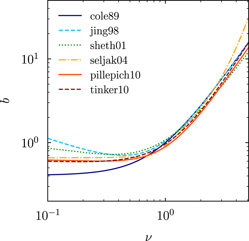
The bias is, in principle, a function of both halo mass and scale, but is expected to become scale-independent at large radii (e.g., Sheth & Tormen 1999; Tinker et al. 2005; Smith et al. 2007). Thus, all bias models implemented in Colossus ignore the scale dependence and quantify the large-scale bias. A simple prediction for the bias can be derived from the peak-background split ansatz (Cole & Kaiser 1989; Mo & White 1996). This model was modified at low masses by Jing (1998), who calibrated their model on simulations of scale-free cosmologies. Sheth et al. (2001) further improved upon the Mo & White (1996) prescription by taking the ellipsoidal nature of the collapse into account. Tinker et al. (2010) undertook a careful numerical calibration and included a prescription for the dependence of bias on the halo mass definition. As a result, their model exhibits a slight redshift dependence for most mass definitions. In addition, a number of numerical calibrations of bias have been undertaken (e.g., Manera et al. 2010; Pillepich et al. 2010). Figure 3 compares the bias models implemented in Colossus as a function of peak height.

Zoom In Zoom Out Reset image size

The most commonly used definition of a halo's boundary and mass is the SO definition, where the radius is defined to enclose a particular overdensity Δ such that

$$\begin{eqnarray}&&{M}_{{\rm{\Delta }}}=\displaystyle \frac{4\pi }{3}{\rm{\Delta }}{\rho }_{\mathrm{ref}}{R}_{{\rm{\Delta }}}^{3},\end{eqnarray} \tag{ 31 }$$

where ${\rho }_{\mathrm{ref}}$ is either the critical or mean matter density of the universe (e.g., Cole & Lacey 1996),

$$\begin{eqnarray}&&{M}_{{\rm{\Delta }}{\rm{m}}}=M(\lt {R}_{{\rm{\Delta }}{\rm{m}}})=\displaystyle \frac{4\pi }{3}{\rm{\Delta }}{\rho }_{{\rm{m}}}(z){R}_{{\rm{\Delta }}{\rm{m}}}^{3},\end{eqnarray} \tag{ 32 }$$

for example, ${R}_{200{\rm{m}}}$ and ${M}_{200{\rm{m}}}$, or

$$\begin{eqnarray}&&{M}_{{\rm{\Delta }}{\rm{c}}}=M(\lt {R}_{{\rm{\Delta }}{\rm{c}}})=\displaystyle \frac{4\pi }{3}{\rm{\Delta }}{\rho }_{{\rm{c}}}(z){R}_{{\rm{\Delta }}{\rm{c}}}^{3},\end{eqnarray} \tag{ 33 }$$

for example, ${R}_{200{\rm{c}}}$ and ${M}_{200{\rm{c}}}$. The labels ${M}_{\mathrm{vir}}$ and ${R}_{\mathrm{vir}}$ indicate a varying overdensity ${{\rm{\Delta }}}_{\mathrm{vir}}(z)$, which Colossus computes using the approximation of Bryan & Norman (1998). Colossus offers a number of basic routines related to SO masses and radii, beginning with the computation of the density threshold ${\rho }_{\mathrm{ref}}$. Based on this threshold, we define a typical velocity

$$\begin{eqnarray}&&{v}_{{\rm{\Delta }}}\equiv \sqrt{\displaystyle \frac{{{GM}}_{{\rm{\Delta }}}}{{R}_{{\rm{\Delta }}}}},\end{eqnarray} \tag{ 34 }$$

which we use to define the dynamical time of the halo as the time it takes to cross $2{R}_{{\rm{\Delta }}}$,

$$\begin{eqnarray}&&{t}_{\mathrm{dyn}}(z)\equiv {t}_{\mathrm{cross}}(z)=\displaystyle \frac{2{R}_{{\rm{\Delta }}}}{{v}_{{\rm{\Delta }}}}={2}^{3/2}{t}_{{\rm{H}}}(z){\left(\displaystyle \frac{{\rho }_{{\rm{\Delta }}}(z)}{{\rho }_{{\rm{c}}}(z)}\right)}^{-1/2}.\end{eqnarray} \tag{ 35 }$$

Notably, this time does not depend on the distribution of matter inside the halo or even the halo radius, but only on ${\rho }_{{\rm{\Delta }}}$ and the Hubble time,

$$\begin{eqnarray}&&{t}_{{\rm{H}}}(z)\equiv \displaystyle \frac{1}{H(z)}=\sqrt{\displaystyle \frac{3}{8\pi G{\rho }_{{\rm{c}}}(z)}}.\end{eqnarray} \tag{ 36 }$$

Alternatively, Colossus offers the time to pericenter (traveling one ${R}_{{\rm{\Delta }}}$) or the orbital time (traveling $2\pi {R}_{{\rm{\Delta }}}$) as definitions of the dynamical time.

If we wish to convert between ${R}_{{\rm{\Delta }}}$ and ${M}_{{\rm{\Delta }}}$ for different overdensity definitions, the results depend on the density profile. In particular, we need to solve Equation (31) numerically given a particular ${\rho }_{\mathrm{ref}}$ and M(r). By default, Colossus uses a Navarro–Frenk–White (NFW) profile (see Section 4.2) to convert between definitions, but the user can also choose other profile models. The concentration can either be given by the user or be automatically computed using a model of the concentration–mass relation (Section 4.3).

The conversion between different overdensity definitions constitutes a special case of a more general conversion where not only the overdensity is varied but also the redshift. Here, the assumption is that the halo density profile is static in time, but that the spherical overdensity (SO) "pseudo-evolves" due to the change in the critical or mean density (see, e.g., Diemand et al. 2005; Cuesta et al. 2008; Diemer et al. 2013; Zemp 2014; More et al. 2015). This more general routine is also implemented in Colossus. All conversion routines are based on the Brent (1973) root finding algorithm with a default accuracy of 10⁻¹².

The density profiles of dark matter halos have been studied extensively in the literature, generally based on the results of numerical simulations. All profile models implemented in Colossus describe the spherically averaged density profile $\rho (r)$. The implementation of each model relies on a base class that numerically computes numerous quantities, including:

• 1.  
  the linear and logarithmic derivatives of density, $d\rho /{dr}$ and $d\mathrm{ln}(\rho )/d\mathrm{ln}(r)$;
• 2.  
  the enclosed mass, $M(\lt r)$;
• 3.  
  the surface density Σ and excess surface density ${\rm{\Delta }}{\rm{\Sigma }}$ (sometimes referred to as "differential surface density"), defined as ${\rm{\Delta }}{\rm{\Sigma }}(R)\equiv {\rm{\Sigma }}(\lt R)-{\rm{\Sigma }}(R)$, where ${\rm{\Sigma }}(\lt R)$ is the average surface density inside R weighted by area,

  $$\begin{eqnarray}&&{\rm{\Sigma }}(\lt R)\equiv \displaystyle \frac{2}{{R}^{2}}{\int }_{0}^{R}r{\rm{\Sigma }}(r){dr};\end{eqnarray} \tag{ 37 }$$
• 4.  
  the circular velocity, ${v}_{{\rm{c}}}(r)=\sqrt{{GM}(\lt r)/r}$, and the maximum circular velocity, ${v}_{\max }$; and
• 5.  
  SO radius and mass for a given overdensity definition and redshift.

A profile model is fully specified by only the density $\rho (r)$. The quantities listed above are, by default, computed numerically from $\rho (r)$ unless a model implementation overwrites them when, for example, analytical solutions are available. In Colossus, the density profile is modeled as the sum of an "inner" profile (or 1-halo term) as well as an arbitrary number of "outer" profiles. The left panels of Figure 4 show a comparison of the inner profile models implemented in Colossus.

• 1.  
  The three-parameter profile of Einasto (1965) is described by a logarithmic slope that changes progressively with radius,

  $$\begin{eqnarray}&&{\rho }_{\mathrm{Einasto}}(r)={\rho }_{{\rm{s}}}\exp \left(-\displaystyle \frac{2}{\alpha }\left[{\left(\displaystyle \frac{r}{{r}_{{\rm{s}}}}\right)}^{\alpha }-1\right]\right).\end{eqnarray} \tag{ 38 }$$

  The user can either choose the shape parameter α or let it be determined by the fitting function of Gao et al. (2008),

  $$\begin{eqnarray}&&\alpha (\nu )=0.155\,+\,0.0095{\nu }^{2},\end{eqnarray} \tag{ 39 }$$

  which gives $\alpha =0.25$ for the massive halo shown in Figure 4.
• 2.  
  The two-parameter Hernquist (1990) profile is given by the expression

  $$\begin{eqnarray}&&{\rho }_{\mathrm{Hernquist}}(r)=\displaystyle \frac{{\rho }_{{\rm{s}}}}{\left(\tfrac{r}{{r}_{{\rm{s}}}}\right){\left(1+\tfrac{r}{{r}_{{\rm{s}}}}\right)}^{3}}.\end{eqnarray} \tag{ 40 }$$

  This profile approaches power laws of slope −1 and −4 at small and large radii, respectively, turning over around the scale radius ${r}_{{\rm{s}}}$.
• 3.  
  The NFW profile (Navarro et al. 1995, 1996, 1997) changes the outer slope of the Hernquist profile to −3,

  $$\begin{eqnarray}&&{\rho }_{\mathrm{NFW}}(r)=\displaystyle \frac{{\rho }_{{\rm{s}}}}{\left(\tfrac{r}{{r}_{{\rm{s}}}}\right){\left(1+\tfrac{r}{{r}_{{\rm{s}}}}\right)}^{2}}.\end{eqnarray} \tag{ 41 }$$
• 4.  
  In order to account for the steepening at the splashback radius (Section 4.4), Diemer & Kravtsov (2014, DK14) combined the Einasto profile at small radii with a steepening function in the outer profile,

  $$\begin{eqnarray}&&{\rho }_{\mathrm{DK}14}(r)={\rho }_{\mathrm{Einasto}}\times {\left[1+{\left(\displaystyle \frac{r}{{r}_{{\rm{t}}}}\right)}^{\beta }\right]}^{-\tfrac{\gamma }{\beta }},\end{eqnarray} \tag{ 42 }$$

  where β determines how rapidly this steepening happens and γ represents the limiting slope of the steepening term. Diemer & Kravtsov (2014) recommend $(\beta ,\gamma )=(4,8)$ or $(6,4)$, depending on how the halo sample was selected (the profile shown in Figure 4 uses $(4,8)$). The turnover radius ${r}_{{\rm{t}}}$ depends on the location of the splashback radius and thus on the mass accretion rate. The DK14 profile makes sense only when combined with a prescription for the outer profile as described below.

Regardless of the parameterization of the given profile, the user can initialize a profile from a mass and concentration that are automatically converted to the native parameters (e.g., ${\rho }_{{\rm{s}}}$ and ${r}_{{\rm{s}}}$). Furthermore, Colossus provides an arbitrary spline-interpolated profile based on a table of either $\rho (r)$ or M(r). Care needs to be taken when integrating over such profiles if, for example, the radial extent of the table is not sufficient to compute the surface density.

Zoom In Zoom Out Reset image size

The left panels of Figure 4 show a comparison of these profile forms and their logarithmic derivatives. All models of the inner profile become somewhat unrealistic at $r\gtrsim {R}_{\mathrm{vir}}$, where the outer profile begins to contribute significantly. Physically, the excess density at large radii is due to a combination of the nonlinear infall of matter into the halo and the statistical contribution from neighboring halos (the 2-halo term, e.g., Smith et al. 2003; Hayashi & White 2008). In Colossus, these contributions are modeled as the sum of an arbitrary combination of the following terms:

• 1.  
  The mean density of the universe, $\rho ={\rho }_{{\rm{m}}}(z)$. This term should always be included if the profile is evaluated at large radii.
• 2.  
  An estimate of the 2-halo term based on the linear matter–matter correlation function,

  $$\begin{eqnarray}&&{\rho }_{2{\rm{h}}}(r,z)={\rho }_{{\rm{m}}}(z)\xi (r,z)b(\nu ),\end{eqnarray} \tag{ 43 }$$

  where the bias $b(\nu )$ can be estimated based on a model of halo bias (Section 3.3). The 2-halo term shown in the right panels of Figure 4 corresponds to b = 6.1, appropriate for a very massive halo.
• 3.  
  A power-law outer profile (e.g., Diemer & Kravtsov 2014) that can be used to approximate the profile of infalling matter (Bertschinger 1985) or mimic a 2-halo term. Mathematically the power-law outer term is described as

  $$\begin{eqnarray}&&{\rho }_{\mathrm{PL}}(r,z)={\rho }_{{\rm{m}}}(z)\displaystyle \frac{a}{\tfrac{1}{{\rho }_{\max }}+{\left(\tfrac{r}{{r}_{\mathrm{pivot}}}\right)}^{b}},\end{eqnarray} \tag{ 44 }$$

  where a is a normalization, b is the slope, and ${r}_{\mathrm{pivot}}$ is an arbitrary pivot radius that can be set to either a fixed radius or an SO radius. The limiting density ${\rho }_{\max }$ is introduced to avoid spurious contributions at small radii. The power-law outer profile shown in Figure 4 has a = 1 and b = 1.5 (Diemer & Kravtsov 2014).

Finally, the density profile object provides powerful functionality to fit profile models to data. The data can be density, enclosed mass, or (excess) surface density. Estimates of the uncertainties on those data and their covariances are taken into account if desired, and the fit can be performed using either a least-squares or MCMC algorithm (Goodman & Weare 2010).

As illustrated in the previous section, the most popular expressions for halo density profiles are characterized by a scale radius, ${r}_{{\rm{s}}}$. Such profiles are more naturally described by an SO mass and a concentration, the ratio between the SO radius and the scale radius, ${c}_{{\rm{\Delta }}}\equiv {R}_{{\rm{\Delta }}}/{r}_{{\rm{s}}}$. If concentration can be quantified as a function of mass and other parameters, a full description of the halo profile can be derived from only an input mass, making the concentration–mass relation a paramount tool in halo modeling. However, the c–M relation turns out to depend on redshift and cosmology in a non-trivial fashion, and to exhibit significant halo-to-halo scatter. Thus, numerous models for the c–M relation have been proposed in the literature. Most works rely on NFW-based concentrations, i.e., fitting halo profiles with the NFW form to derive ${r}_{{\rm{s}}}$, but other parameterizations exist (e.g., Klypin et al. 2011; Prada et al. 2012; see Dutton & Macciò 2014 for a comparison with Einasto-based concentrations).

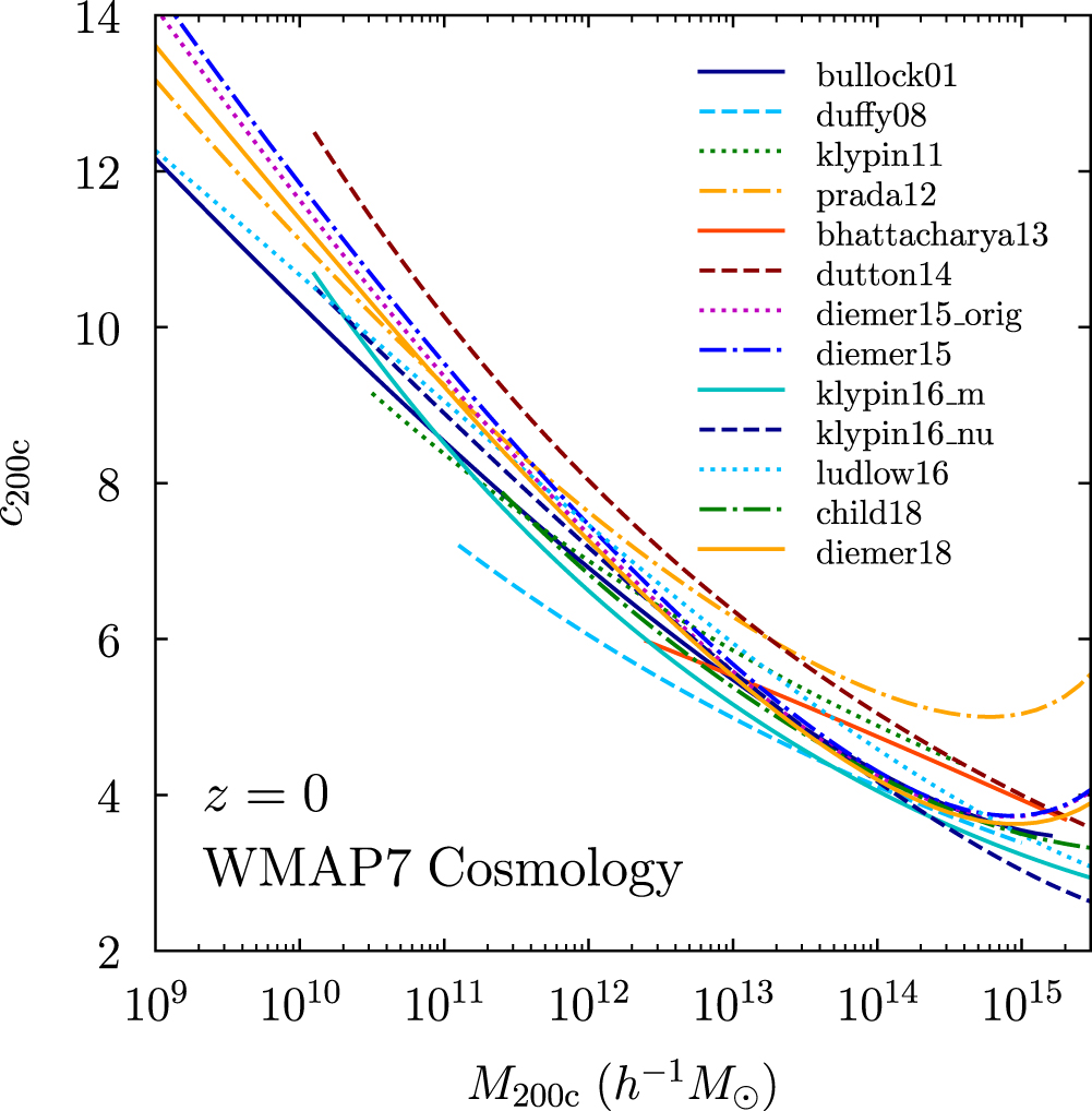
The Colossus concentration module implements several models for the c–M relation (Table 3). Figure 5 shows a comparison of their predictions at z = 0. The models broadly fall into three categories. First, the c–M relation is reasonably well described by a power law for a given redshift and cosmology, and within a certain range of halo mass (Duffy et al. 2008; Klypin et al. 2011, 2016; Dutton & Macciò 2014; Child et al. 2018). Second, concentration is strongly correlated with halo age, giving rise to models that base concentration on a description of halo formation times (e.g., Bullock et al. 2001; Wechsler et al. 2002; Zhao et al. 2003, 2009; Ludlow et al. 2016). Finally, the c–M relation is almost universal with redshift when mass is expressed as peak height (Section 3.1), leading to models that parameterize the dependence either empirically or based on physical arguments (Prada et al. 2012; Bhattacharya et al. 2013; Diemer & Kravtsov 2015; Diemer & Joyce 2018). Some noteworthy models are not implemented in Colossus, most commonly because they are not based on simple analytical expressions and thus demand significant computation (e.g., Eke et al. 2001; Zhao et al. 2009; Correa et al. 2015).

Zoom In Zoom Out Reset image size

A further complication arises because the models quantify different definitions of concentration, including ${c}_{200{\rm{m}}}$, ${c}_{200{\rm{c}}}$, and ${c}_{\mathrm{vir}}$. The conversion to the desired mass definition is performed automatically by Colossus and can be based on either NFW or DK14 profiles. This process is iterative because an input mass in one definition may lead to an output concentration in another definition, which in turn changes the conversion between the masses. The conversion can introduce slight inaccuracies into the predictions for concentration because the profile models do not describe real halos perfectly (Diemer & Kravtsov 2015). Moreover, the c–M relations measured in simulations depend on technical details such as the fitting procedure and binning (Dooley et al. 2014; Meneghetti et al. 2014). Taking these effects into account would add significant complication and is beyond the scope of Colossus.

The splashback radius, ${R}_{\mathrm{sp}}$, has recently been proposed as a physically motivated definition of the halo boundary (Adhikari et al. 2014; Diemer & Kravtsov 2014; More et al. 2015) and has since been observed in stacked cluster density profiles (More et al. 2016; Baxter et al. 2017; Chang et al. 2018). Unlike SO radii, the splashback depends on the dynamical state of a halo, namely on its mass accretion rate. A number of models for this dependence, and additional dependencies on halo mass and redshift, have been proposed (Table 3). Colossus provides a general function to evaluate the model predictions for the splashback radius, splashback mass, enclosed overdensity, and the scatter in those quantities. Figure 6 compares the model predictions for the splashback radius of halo with ${M}_{200{\rm{m}}}={10}^{14}\,{h}^{-1}{M}_{\odot }$ at z = 0.

Zoom In Zoom Out Reset image size

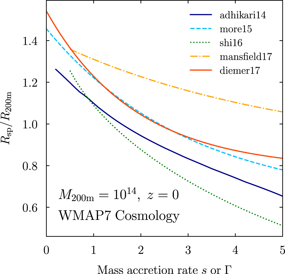
The semi-analytical models of Adhikari et al. (2014) and Shi (2016) are based on spherically collapsing shells whose radial trajectories are integrated numerically. While the Adhikari et al. (2014) model predicts that ${R}_{\mathrm{sp}}$/${R}_{200{\rm{m}}}$ should depend only on the mass accretion rate $s\equiv d\mathrm{ln}(M)/d\mathrm{ln}(a)$, the Shi (2016) model also predicts an evolution with redshift. Numerical calibrations have shown that ${R}_{\mathrm{sp}}$/${R}_{200{\rm{m}}}$ does depend on redshift, regardless of the way ${R}_{\mathrm{sp}}$ is measured: from stacked density profiles (More et al. 2015), non-spherical splashback shells (Mansfield et al. 2017), or particle orbits (Diemer 2017; Diemer et al. 2017). In these calibrations, the mass accretion rate is defined as

$$\begin{eqnarray}&&{\rm{\Gamma }}\equiv \displaystyle \frac{{\rm{\Delta }}\mathrm{ln}(M)}{{\rm{\Delta }}\mathrm{ln}(a)}\end{eqnarray} \tag{ 45 }$$

because the instantaneous rate is not a well-defined quantity in simulations. The time interval over which the mass accretion rate is measured has also varied slightly between the different models but is generally close to a dynamical time. The different definitions of the mass accretion rate complicate the interpretation of the comparison in Figure 6.