Surface Rotation and Photometric Activity for Kepler Targets. I. M and K Main-sequence Stars

A. R. G. Santos; R. A. García; S. Mathur; L. Bugnet; J. L. van Saders; T. S. Metcalfe; G. V. A. Simonian; M. H. Pinsonneault

doi:10.3847/1538-4365/ab3b56

1. Introduction

Stellar rotation is a key ingredient for the generation of magnetic fields and magnetic cycles in the Sun and other solar-type stars (e.g., Brun & Browning 2017). Stars are observed to spin down as they evolve and lose angular momentum (e.g., Wilson 1963; Wilson & Skumanich 1964). Therefore, rotation can also be used as a diagnostic for stellar age, in what we call gyrochronology (e.g., Skumanich 1972; Barnes 2003, 2007; Mamajek & Hillenbrand 2008; García et al. 2014a; Davies et al. 2015; Metcalfe & Egeland 2019). To calibrate the empirical gyrochronology relations, rotation-period estimates for large sample stars are needed as well as precise ages estimates.

Thanks to the NASA mission Kepler, almost 200,000 stars were observed almost continuously for up to four years. These long-duration photometric observations obtained with high precision allow us to measure rotation periods through the modulation of the stellar brightness caused by the passage of spots on the stellar disk. This has been done on a large number of stars observed by Kepler using different techniques, such as periodogram analysis (e.g., Nielsen et al. 2013; Reinhold et al. 2013), autocorrelation function (ACF; e.g., McQuillan et al. 2013b, 2014), and time–frequency analysis with wavelets (e.g., García et al. 2014a). Based on simulated data, the comparison of different pipelines developed to retrieve surface rotation periods using photometric data showed that a combination of different techniques such as those used in García et al. (2014a) and Ceillier et al. (2016, 2017) provides the most complete and reliable set of rotation-period estimates (see details in Aigrain et al. 2015).

Ages can be constrained from gyrochronology relations. However, these relations are calibrated, requiring targets with known ages from independent methods. This is the reason why stars belonging to clusters have been used in the past (e.g., Meibom et al. 2011a, 2011b, 2015). Asteroseismology has proven to be a powerful tool to provide precise stellar ages (e.g., Mathur et al. 2012; Metcalfe et al. 2014; Silva Aguirre et al. 2015; Creevey et al. 2017; Serenelli et al. 2017), and we can now test and improve those relations with a large number of field stars. This led to the results of van Saders et al. (2016) who found that solar-like stars older than the Sun rotate faster than predicted by the classical gyrochronology relations (see also Angus et al. 2015). The authors suggested that this could be the result of the weakening of the magnetic braking when the Rossby number of the star (the ratio between the rotation period and the convective turnover time) reaches a given value. Thus, gyrochronology may not be a uniformly suitable technique for all main-sequence stars, and the apparent weakened braking has implications for the dynamo theory. van Saders et al. (2019) suggested that signatures of this weakened braking might be visible in large samples of field stars with measured rotation periods. However, these relations are still valid for young main-sequence stars. Note that gyrochronology is also not suitable for pre-main-sequence and early-spectral-type stars (e.g., Kraft 1967; Gallet & Bouvier 2013; Epstein & Pinsonneault 2014; Amard et al. 2016).

One of the largest analyses of the surface rotation of main-sequence stars observed by Kepler was performed by McQuillan et al. (2014). They looked for rotation periods in a sample of 133,030 targets using Quarters 3 to 14 and obtained reliable values for 34,030 stars. They estimated ages by comparing their field population to empirical gyrochrones and found that the most slowly rotating stars were consistent with a gyrochronological age of 4.5 Gyr.

In this work, we perform a similar analysis focusing on 26,521 M and K dwarfs observed by Kepler. We use the longest time-series available: up to Kepler Quarter 17, while McQuillan et al. (2014) used only 11 Kepler Quarters. We calibrate the light curves using our own independent software, which high-pass filters the data using filters of 20, 55, and 80 days, preventing us from measuring a harmonic of the real rotation period. In addition, we analyze the Presearch Data Conditioning-Maximum A Posteriori (PDC-MAP; e.g., Jenkins et al. 2010; Smith et al. 2012; Stumpe et al. 2012) light curves to be sure that the rotational modulation detected does not result from photometric pollution by nearby stars. We are particularly careful to remove possible polluters such as red giants, classical pulsators (CPs), and eclipsing binary systems, which can result in the detection of a spurious periodicity. The sample selection and data calibration are described in Section 2. We then apply our rotation pipeline (Section 3) that consists of the combination of the ACF, the wavelet analysis, and the composite spectrum (CS; a combination of the two former methods) to derive the most reliable periods. Our analysis allows us to retrieve rotation periods for more than 4000 additional targets in comparison with the analysis in McQuillan et al. (2014). In particular, we are able to retrieve rotation periods for both fainter and cooler stars. We then measure the photometric magnetic activity proxy S_ph (Section 4). Finally, we interpret the results in Section 5 in terms of rotation, activity, mass, and temperature relations, and conclude in Section 6.

2. Data Preparation and Sample Selection

2.1. Data Preparation

The light curves are obtained from Kepler pixel-data files using large custom apertures that produce stable light curves. For each pixel in the pixel-data file, a reference flux value is computed as the 99.9^th percentile of the flux. Starting from the center of the point-spread function of the target-pixel mask, new pixels are added in one direction of the mask if two conditions are fulfilled: (1) the reference flux of the pixel is higher than a threshold of 100e⁻ s⁻¹; and (2) the flux is smaller than the value of the previous pixel within a small tolerance. In most cases, this second condition allows us to remove the pixels corresponding to a second star present in the aperture.

The resulting light curve is processed through the implementation of the Kepler Asteroseismic Data Analysis and Calibration Software (KADACS; García et al. 2011). KADACS corrects for outliers, jumps, and drifts, and it properly concatenates the independent Kepler Quarters on a star-by-star basis. It also fills the gaps shorter than 20 days in long-cadence data following in-painting techniques based on a multi-scale cosine transform (García et al. 2014b; Pires et al. 2015). The resulting light curves are high-pass filtered at 20, 55 (quarter-by-quarter), and 80 days (using the entire light curve), yielding three different light curves for each target. For light curves longer than one month, KADACS corrects for discontinuities at the edges of the Kepler Quarters. Hereafter, we will refer to KADACS data products, which are optimized for seismic studies, as KEPSEISMIC.⁹

To correctly prepare the Kepler Objects of Interest (KOI) light curves for seismic analysis, we used the published ephemeris of each star from the Mikulski Archive for Space Telescopes (MAST) to remove the transits and interpolate the resultant gaps using the same in-painting techniques mentioned above.

In the analysis below, we compare the results for the different high-pass filters to determine the final stellar rotation period. However, we note that the longer-period filters are also less effective at removing long periodicity instrumental trends from the light curves, including the Kepler yearly modulation.

In our analysis, to ensure that the correct rotation period is retrieved, we also use PDC-MAP light curves from Data Release 25. The comparison between the KEPSEISMIC and PDC-MAP light curves also helps to identify light curves with photometric pollution from nearby stars. We typically construct the KEPSEISMIC light curves using larger apertures than those of the PDC-MAP time-series, which leads to an increase in the number of polluted light curves. Nevertheless, a significant number of light curves show evidence of pollution or multiple signals in both the KEPSEISMIC and PDC-MAP data sets (see Section 2.2, and Tables 4 and 5). To properly understand the source of pollution and/or multiple signals (e.g., possible binary or just nearby star in the field of view) further analyses are needed and currently beyond the scope of this study. Note that, in addition to the difference in the aperture sizes, the PDC-MAP light curves are calibrated quarter-by-quarter while the KEPSEISMIC light curves are calibrated using all of the quarters at once. Furthermore, the PDC-MAP light curves are often high-pass filtered at a period of 20 days, which can lead to biased results (see Appendix B).

2.2. Sample Selection

We analyze long-cadence (Δt = 29.42 minutes) data of M and K main-sequence stars observed during the main mission of the Kepler satellite (Borucki et al. 2010). The targets were selected according to the Kepler Stellar Properties Catalog for Data Release 25 (KSPC DR25; Mathur et al. 2017), where M dwarfs have effective temperatures ${T}_{\mathrm{eff}}$ smaller than 3700 K and K dwarfs have temperatures within 3700 and 5200 K. The initial sample is composed of 26,521 targets (24,171 K stars and 2350 M stars) shown in Figure 1.

**Figure 1.** Surface gravity-effective temperature diagram of the 26,521 M and K dwarfs according to KSPC DR25 (Mathur et al. 2017), color-coded by the number of stars in each bin. The sizes of the ${T}_{\mathrm{eff}}$ and $\mathrm{log}\,g$ bins are ∼16 K and ∼7 × 10⁻³ dex, respectively. For context, other stars in KSPC DR25 are plotted in gray. Effective temperature ( ${T}_{\mathrm{eff}}$ ) and surface gravity ( $\mathrm{log}\,g$ ) values are adopted from KSPC DR25.
Download figure:
Standard image High-resolution image

**Figure 1.** Surface gravity-effective temperature diagram of the 26,521 M and K dwarfs according to KSPC DR25 (Mathur et al. 2017), color-coded by the number of stars in each bin. The sizes of the ${T}_{\mathrm{eff}}$ and $\mathrm{log}\,g$ bins are ∼16 K and ∼7 × 10⁻³ dex, respectively. For context, other stars in KSPC DR25 are plotted in gray. Effective temperature ( ${T}_{\mathrm{eff}}$ ) and surface gravity ( $\mathrm{log}\,g$ ) values are adopted from KSPC DR25.
Download figure:
Standard image High-resolution image

We expect a number of different polluters in the sample of main-sequence M and K stars. These polluters will display stellar variability due to pulsations, eclipses, or other astrophysical variability not related to spot modulation. Therefore, we search and identify such polluters.

We start by removing the known eclipsing binaries (a total of 272 stars in the Villanova Kepler Eclipsing Binary Catalog; Abdul-Masih et al. 2016; Kirk et al. 2016) and known RR Lyrae (three stars in this sample; R. Szabó et al. 2019, in preparation). These are listed in Table 4. For rotational analysis of eclipsing binaries, see Lurie et al. (2017).

We also remove possible misclassified red giants (listed in Table 4; R. A. García et al. 2019, in preparation). A significant fraction of those were identified by Berger et al. (2018) using astrometric data from Gaia (Gaia Data Release 2; Gaia Collaboration et al. 2018). The remainder of the misclassified targets were identified using the hallmark signature of red-giant stars in light curves: the presence of red-giant oscillations. We use both neural-network and machine-learning techniques that automatically identify power spectra consistent with red-giant stars (see Bugnet et al. 2018; Hon et al. 2018) and/or by visual examination for red-giant pulsations. In total, 1221 misclassified red giants were removed from the subsequent rotation analysis. Thirty of those targets are also identified as eclipsing binaries (flagged accordingly in Table 4), which may suggest that one of the components of the binary is a red giant.

Another group of potential polluters in the sample corresponds to light curves exhibiting evidence of photometric pollution possibly from nearby stars in the field of view. We consider light curves to be photometrically polluted when the signal is only present in some Kepler Quarters, namely every four Quarters.¹⁰ We also identify targets as photometrically polluted when their light curves contain a signal or multiple signals only in the KEPSEISMIC time-series. As mentioned previously, the apertures used for the KEPSEISMIC data sets are typically larger than those of the PDC-MAP data sets, and thus more likely to be affected by the contribution of background stars in the field of view. In total, we have flagged the light curves of 255 targets as photometrically polluted (Table 4).

Targets with multiple signals in both the PDC-MAP and KEPSEISMIC light curves are likely to be associated with different unresolved sources. Although determining whether these targets are true binary systems or merely polluted by background stars is beyond the scope of this work, we perform a rotation analysis of these light curves (Table 5). In total, we have identified 270 targets with multiple signals in both the KEPSEISMIC and PDC-MAP data sets.

Another concern is pollution by possible CP that were not previously identified. We start by flagging the targets that exhibit multiple high-amplitude peaks at relatively high frequencies (higher than 3.5 μHz) in the power-density spectrum, which are typical of CPs. Then, we visually check those targets and all of the other targets for which the rotation estimate (from Section 3.1) is shorter than 10 days. We only flag stars as CP candidates when there are more than three associated peaks in the power spectra.

We also distinguish between three types of CP candidates. Type-1 candidates (left panels of Figure 2) show a behavior somewhat similar to RR Lyrae and Cepheids (see, e.g., R. Szabó et al. 2019, in preparation; Kolenberg et al. 2010; Moskalik et al. 2015): high-amplitude and stable flux variations, beating patterns, and a large number of harmonics. Interestingly, a significant fraction of these targets were identified as Gaia binary candidates in Berger et al. (2018) and Simonian et al. (2019). In particular, Simonian et al. (2019) focused on tidally synchronized binary systems. Of the 74 Type-1 candidates we identify common to their analysis, 51 are found to be possible synchronized binaries. Therefore, it is possible that these targets are not CPs but close-in binaries (CB). If that is the case, the signal may still be related to rotation, but may be distinct from the rotational behavior of single stars. For the remainder of this paper, we refer to these targets (350) as Type-1 CP/CB candidates. Type-1 CP/CB candidates are listed and flagged in Table 3. Targets marked as Type-2 CP/CB candidates (nine stars; middle panel of Figure 2) exhibit a large number of harmonics in the power spectrum, similarly to Type-1 CP/CB candidates. However, these targets differ from Type 1, in particular, in that the highest peak in the periodogram is the second harmonic associated with the signal instead of the first harmonic (period of the signal). This signature may also be consistent with contact binary systems (see, e.g., Lee et al. 2016; Colman et al. 2017). Therefore, similarly to Type 1, these targets are flagged as CP/CB candidates. The power spectrum of Type-3 CP candidates (nine stars; right panel of Figure 2) resembles those of γ Doradus or δ Scuti, depending on characteristic frequencies and nature of the modes (see, e.g., Bradley et al. 2015; Van Reeth et al. 2015; Barceló Forteza et al. 2017). A proper analysis of these targets is, however, beyond the scope of this work. Type-2 and -3 candidates are listed in Table 4.

We do not provide rotation periods for confirmed RR Lyrae, misclassified red giants, eclipsing binaries, light curves with photometric pollution, or Type-2 and -3 CP/CB candidates. This leaves us with 24,782 stars for the rotational analysis. Table 1 summarizes the number of polluters and targets used in the subsequent analysis.

Table 1. Summary of Targets Classified as M and K Dwarfs in KSPC DR25 (Mathur et al. 2017)

M dwarfs	2156
K dwarfs	22,006
Type-1 CP/CB candidates	350
Multiple signals	270

Eclipsing Binaries (EB)	242
Red giants (RG)	1191
EB and RG	30
RR Lyrae	3
Photometric pollution	255
Type-2 and -3 CP/CB candidates	18

Note. The top part of the table corresponds to the targets for which we perform the rotational analysis, while the polluters summarized in the bottom part are not used for the rotational analysis.

Download table as: ASCII Typeset image

Finally, possible additional non-single non-main-sequence M and K stars are flagged in Tables 3–5 but not removed from the analysis. We add subgiant and binary flags from Berger et al. (2018; Gaia DR2), a synchronized binary flag from Simonian et al. (2019), and a FliPer_Class flag (see Bugnet et al. 2019), which indicates solar-type stars, CPs, and binary/photometric pollution. We do not remove these targets from the analysis, but we alert the reader to this possible pollution.

3. Surface Rotation Detection

In Section 3.1, we present the methodology implemented to estimate the surface rotation period. Sections 3.1.1 and 3.1.2 summarize the results from the automatic selection and visual examination, respectively.

3.1. Methodology to Retrieve Rotation Periods

To extract the rotation-period estimates, we implement the methodology described in Ceillier et al. (2016, 2017). It combines a time–frequency analysis and the ACF. This methodology was found by Aigrain et al. (2015) to have the best performance in terms of completeness and reliability compared to the periodogram analysis alone, ACF alone, or a combination between the two and spot modeling.

Despite the fact that our KEPSEISMIC light curves have been corrected for instrumental effects (see Section 2.1; García et al. 2011), calibrated light curves may still exhibit instrumental modulations. We therefore remove Kepler Quarters with anomalously high variance compared with their neighbors from the rotation analysis (see García et al. 2014a).

First, we estimate periods from a time-period analysis using the wavelet decomposition (Torrence & Compo 1998) adapted by Mathur et al. (2010) using the correction by Liu et al. (2007). The wavelet analysis assesses the correlation between the mother wavelet and the rebinned data (to decrease the computing time) by sliding the wavelet in time for a given period of the wavelet. The range of periods is probed through an iterative process. For the mother wavelet, we use the Morlet wavelet, which is the convolution between a sinusoidal and a Gaussian function. This analysis provides the wavelet power spectrum (WPS). An example is given in panel (b) of Figure 3, where red and black indicate high power, while blue indicates low power. The visual inspection of the WPS also helps us to determine whether the signal is present along the time-series or if an artifact resulting from instrumental noise at a particular time is present. The black hashed area indicates the cone of influence that marks the limit on observing at least four rotations in the light curve. Rotation signals found inside the cone have a lower confidence level. Finally, we obtain the global wavelet power spectrum (GWPS) by computing the sum of the WPS along time for each period of the wavelet (panel c) of Figure 3. We then fit the GWPS, through a least-squares minimization, with multiple Gaussian functions. The rotation estimate from the wavelet analysis corresponds to the central period of the highest fitted period peak, while the uncertainty corresponds to the half width at half maximum (HWHM) of the corresponding Gaussian profile. Computed in this way, the inferred uncertainty also accounts for possible differential rotation.

**Figure 3.** Rotation analysis for KIC 4918333. (a) KEPSEISMIC light curve obtained with the 55 day filter. (b) Wavelet power spectrum (WPS) where red and black correspond to high power and blue to low power. The cone of influence is shown by the black crossed area. (c) Global wavelet power spectrum (GWPS; black) and corresponding best fit with multiple Gaussian functions (red). (d) ACF (black) of the light curve and smoothing ACF (red). (e) Composite spectrum (black) and respective fit with multiple Gaussian profiles (red). For the GWPS, ACF, and CS, the black dotted lines mark the respective rotation-period estimates.
Download figure:
Standard image High-resolution image

Our second method for measuring periods consists of the ACF of light curves (ACF; following the procedure in McQuillan et al. 2013a), which was combined with wavelet analysis for the first time in García et al. (2014a). The ACF is smoothed using a Gaussian function whose width is a tenth of the most significant period selected from the Lomb–Scargle periodogram (Lomb 1976; Scargle 1982) of the ACF. We identify the significant peaks and take the highest peak as the rotation-period estimate from the ACF. We also examine the ACF for evidence of double-peaked features resulting from active regions in anti-phase. Panel (d) of Figure 3 shows the ACF for a given target in the sample.

Finally, the third method of estimating rotation period utilizes the CS, which combines the GWPS and the ACF as described by Ceillier et al. (2016, 2017). The CS corresponds to the product of the normalized GWPS and the normalized ACF resampled in the same period of the GWPS. Periods present in both methods, GWPS and ACF, are enhanced by the CS, allowing for a better identification of the intrinsic rotation periods of the star. We also fit the CS with multiple Gaussian functions; the central period and HWHM of the profile corresponding to the highest peak are taken as its period estimate and uncertainty. Panel (e) of Figure 3 shows an example of the CS.

For the rotation-period estimate provided in Tables 3 and 5, we prioritize the value returned by the wavelet analysis. When the WPS does not allow us to successfully recover the rotation period, we provide the value recovered from the CS. If both WPS and CS fail to infer the rotation period, the rotation period provided is that found by the ACF without uncertainty. Note that the primary goal of the ACF and CS is to validate the rotation period and better identify the reliable results.

3.1.1. Automatic Selection

Having the rotation-period estimates from the GWPS, ACF, and CS for the three sets of KEPSEISMIC light curves, we start by selecting the targets with the most reliable rotation estimates.

For the automatic selection, the appropriate filter is chosen according to the rotation period. We note that it is still possible to recover periods longer than the cut-off period of the filter. The transfer function is unity below the cut-off period. Above that, it varies sinusoidally and slowly approaches zero at twice of the cut-off period. Therefore, the amplitude of rotation periods that are slightly longer than the cut-off period would be only slightly reduced, while rotation periods close to 1.5 times the cut-off period would have roughly half of the original amplitude. It is therefore still possible to extract a high signal-to-noise ratio, reliable peak of a period 1.5 times the cut-off period using our rotation pipeline. However, the 80 day filtered light curves are the least stable, often exhibiting instrumental modulations and, thus, we only use them in the automatic selection for rotation periods longer than 60 days. For rotation periods shorter than 23 days, priority is given to the period estimate obtained from the 20 day filter. For rotation periods between 23 and 60 days, the primary filter is the 55 day filter, while for longer periods, priority is given to the 80 day filter.

The targets with reliable rotation-period estimates are automatically selected if:

1.
for a given filter, the rotation-period estimates from GWPS, ACF, and CS agree within 2σ where σ is chosen to be the period uncertainty from GWPS;
2.
the rotation-period estimates agree within 20% between different filters
- (a)
  for P_rot < 60 days, the rotation estimates agree between the 20 day and 55 day filters;
- (b)
  or for P_rot ≥ 60 days, the rotation estimates agree between the 55 day and 80 day filters;
3.
for the appropriate filter, the peak height in the ACF and CS are larger than a given threshold. We adopt the thresholds imposed by Ceillier et al. (2017):
- (a)
  G_ACF ≥ 0.2, where G_ACF is the height of the ACF peak that corresponds to P_rot;
- (b)
  H_ACF ≥ 0.3, where H_ACF is the mean difference between the height of the ACF peak and the values of the two local minima on either side of the peak;
- (c)
  and H_CS ≥ 0.15, where H_CS is calculated in the same manner as H_ACF but for the CS.

Following the steps above, 9586 targets were automatically selected (this number includes Type-1 CP/CB candidates), which corresponds to ∼60% of the total number of targets for which we provide rotation-period estimates (Table 3). Targets whose retrieved period is consistent with the reported orbital periods for confirmed and candidate planet hosts (data from the Exoplanet Archive) are reported as targets with no spot modulation (Table 4).

3.1.2. Visual Check

For stars that were not automatically selected, we proceed to visually check their KEPSEISMIC (three filters) and PDC-MAP light curves, the respective power-density spectra, and the rotation diagnostics. We also visually check the light curves of the targets for which the rotation results for the PDC-MAP light curves are not consistent with those for the KEPSEISMIC light curves. Often, half of the rotation period is recovered from the PDC-MAP time-series (see Appendix B). This is probably due to the fact that PDC-MAP applies a 20 day filter, but not systematically in all quarters or to all stars. The comparison with PDC-MAP also helps to identify KEPSEISMIC light curves polluted by nearby stars, as the latter use larger apertures (see Section 2.1). Targets showing evidence for photometric pollution are listed in Table 4.

Although multiple signals present in both the KEPSEISMIC and PDC-MAP light curves may still be the result of photometric pollution by background stars, we determine and report the periods of the observed multiple signals (Table 5). Note that these multiple signals are most likely not related to differential rotation, as the detected periods are well separated. For most of these targets, the periods of the different signals have to be determined through visual inspection and manually, for example, by limiting the range of period to be searched. For some of the targets, one of the multiple signals is consistent with one of the CP/CB candidates described above. Thus, we also provide the respective flag in Table 5. For signals consistent with Type 2 and 3, we do not provide a period. Finally, we note that some of the signatures can be the result of eclipses or transits. Although some of the targets with multiple signals are KOIs reported as false negatives, none of these targets is a confirmed eclipsing binary.

The rotation-period estimate in Tables 3 and 5 is provided as described in Section 3.1, prioritizing the results from the wavelet analysis.

From the visual inspection, the rotation periods for 6,324 additional targets were determined. In total, we provide rotation-period estimates for 15,910 targets (Tables 3–5; including Type 1 CP/CB candidates and light curves with multiple signals).

Although a significant number of targets exhibit evidence for rotational modulation (3562), we are not able to confidently recover rotation periods. Generally, their light curves exhibit instrumental effects, which hamper the detection of the true rotation period. We mark these in Table 4 as targets with possible spot modulation.

From this analysis, we find that 5310 targets (also listed in Table 4) show no evidence for spot modulation. This could be due to the combination of small-amplitude spot modulation and noise, or due to the spot visibility, which depends on the stellar inclination angle and spot latitudinal distribution.

The results from the rotational analysis are summarized in Table 2.

Table 2. Summary of the Results from the Rotational Analysis of 24,782 Targets

With ${P}_{\mathrm{rot}}$ Estimate
	Auto. selected	Visually selected
M dwarfs	918	612
K dwarfs	8380	5380

Type-1 CP/CB candidates 350

Multiple signals 270

Without ${P}_{\mathrm{rot}}$ estimate

	No rotation	Possible rotation
M dwarfs	494	132
K dwarfs	4816	3430

Note. The top part of the table corresponds to the targets for which we provide an P_rot estimate (automatically and visually selected). The bottom part of the table corresponds to the targets for which we do not provide an P_rot estimate. Some of those targets do not exhibit spot modulation while others show possible spot modulation, but we are unable to confidently provide a P_rot value.

Download table as: ASCII Typeset image

4. Photometric Magnetic Activity Proxy

Using Convection, Rotation, and planetary Transits (CoRot; Baglin et al. 2006) data for the solar-type star HD 49933, García et al. (2010) showed that the light-curve variability due to the presence of magnetic features on the stellar surface—including starspots—provides a proxy of stellar magnetic activity. However, brightness variations may include contributions from different phenomena, such as active regions, granulation, oscillations, stellar companions, or instrumental effects. Different phenomena affect the light curve at different timescales. Therefore, to properly estimate a photometric magnetic activity proxy, the stellar rotation period must be taken into account. Mathur et al. (2014) determined that the activity proxy ${S}_{\mathrm{ph}}$ computed as the standard deviation of subseries of length 5 × P_rot provides a reasonable measure of activity and is primarily related to magnetism and minimizes the contributions from other sources of variability. Furthermore, using the Variability of Solar Irradiance and Gravity Oscillations (VIRGO; Fröhlich et al. 1995) and Global Oscillations at Low Frequency (GOLF; Gabriel et al. 1995) data, the photometric activity proxy ${S}_{\mathrm{ph}}$ was shown to recover the variation associated with the solar activity cycle at both 11 yr and quasi-biennial timescales (Salabert et al. 2017). For seismic solar-analog stars observed by Kepler and by the ground-based, high-resolution Hermes spectrograph (Raskin et al. 2011), Salabert et al. (2016) demonstrated that ${S}_{\mathrm{ph}}$ measurements are consistent with the chromospheric activity index measured from the Ca K-line emission (Wilson 1978).

Thanks to the Kepler space mission, the photometric activity can be easily estimated through ${S}_{\mathrm{ph}}$ for a large number of stars with known rotation periods (which we estimate here). This is a clear advantage in relation to chromospheric activity indices, which require a large amount of ground-based telescope time and are only possible to measure for bright targets. However, the photometric variability depends on the visibility of active regions. For example, assuming a similar latitudinal distribution of active regions in the Sun for other solar-type stars (note that it may not be true for late-type M dwarfs), ${S}_{\mathrm{ph}}$ will correspond to a lower limit of the true photometric activity level for stars with small inclination angles, i.e., the angle between the rotation axis and the line of sight, which is unknown for most targets.

In this work, we compute the photometric activity index ${S}_{\mathrm{ph}}$ for the M and K dwarfs with period estimates obtained in Section 3. In Tables 3 and 5, the ${S}_{\mathrm{ph}}$ value and respective uncertainty are provided as the mean value and standard deviation of the ${S}_{\mathrm{ph}}$ computed over subseries of length 5 × P_rot. The ${S}_{\mathrm{ph}}$ index is corrected for the photon noise following the approach by Jenkins et al. (2010). However, for 1% of the targets with P_rot estimate, the correction from Jenkins et al. (2010) leads to negative ${S}_{\mathrm{ph}}$ values. For such targets, the correction to the photon noise is instead computed from the flat component in the power-density spectra. In Table 5 (light curves with multiple signals), the multiple ${S}_{\mathrm{ph}}$ values for a given target may change significantly as they are computed at different timescales depending on the respective period.

5. Results

Following the methodology described in Section 3, surface rotation periods were successfully measured for 15,290 stars (∼62% of the targets for which we perform the rotational analysis; 1530 M and 13,760 K dwarfs), and for additional 350 Type-1 CP/CB candidates and 270 targets whose light curves show multiple signals. The photometric activity proxy ${S}_{\mathrm{ph}}$ was also measured for the same targets.

Tables 3 and 5 summarize the properties and results for the stars with rotation-period estimates, including Type-1 CP/CB candidates and those light curves with multiple signals in both the KEPSEISMIC and PDC-MAP data sets. Table 4 lists the remainder of the target sample.

Figure 4 compares the distribution of Kepler magnitudes (Kp) for targets with rotation-period estimate with those for CP/CB candidates (Type 1, 2, and 3), targets with possible spot modulation, and targets without evidence for spot modulation. The magnitude of stars with possible rotation modulation and of CP/CB candidates is consistent with that of stars with successful rotation measurement. For CP/CB candidates, there is, however, a slight excess of brighter targets. The distribution of targets that do not exhibit spot modulation extends to fainter magnitudes than that of targets with rotation estimates. Faint targets often show high levels of noise which hampers detection of rotational signatures.

Type-1 CP/CB candidates and targets whose light curves show multiple signals are neglected in Figures 5–9, as are all of the possible non-single non-main-sequence stars flagged by Berger et al. (2018), Simonian et al. (2019), and FliPer_Class (Bugnet et al. 2019). In Appendix A, we present the same figures where all targets in Tables 3 and 5 are considered.

**Figure 5.** Distribution of rotation periods (left panels) and ${S}_{\mathrm{ph}}$ values (right panels) for M (top panels) and K dwarfs (bottom panels) shown in red. The respective median values are marked by the dotted lines. The distributions and corresponding median values for the full subsample of M and K dwarfs with P_rot estimate are shown by the black solid and dashed lines, respectively.
Download figure:
Standard image High-resolution image

**Figure 5.** Distribution of rotation periods (left panels) and ${S}_{\mathrm{ph}}$ values (right panels) for M (top panels) and K dwarfs (bottom panels) shown in red. The respective median values are marked by the dotted lines. The distributions and corresponding median values for the full subsample of M and K dwarfs with P_rot estimate are shown by the black solid and dashed lines, respectively.
Download figure:
Standard image High-resolution image

**Figure 6.** Rotation period as a function of effective temperature (left panel) and mass (right panel) color-coded by the number of stars in a given parameter range. Brighter colors indicate higher density regions than darker colors. Stellar effective temperature and mass are taken from KSPC DR25.
Download figure:
Standard image High-resolution image

**Figure 7.** Photometric activity index ${S}_{\mathrm{ph}}$ as a function of effective temperature (left panel) and mass (right panel) color-coded by the number of stars in a given parameter range. Stellar effective temperature and mass are taken from KSPC DR25.
Download figure:
Standard image High-resolution image

**Figure 8.** Comparison between the stellar masses from McQuillan et al. (2014; Mass_McQ) and Mathur et al. (2017; Mass_{KSPC DR25}).
Download figure:
Standard image High-resolution image

**Figure 9.** Photometric activity proxy as a function of the rotation period color-coded by the number of stars in a given parameter range for: all M and K dwarfs (top panel), M dwarfs (middle panel), and K dwarfs (bottom panel). For comparison, the ${S}_{\mathrm{ph}}$ values at solar activity maximum (314.5 ppm) and minimum (67.4 ppm) are marked by the dashed green lines. Solar values from Mathur et al. (2014).
Download figure:
Standard image High-resolution image

Figure 5 summarizes the results for the targets with period estimate. M dwarfs have, on average, longer rotation periods and larger ${S}_{\mathrm{ph}}$ values than K dwarfs, which is consistent with the results in McQuillan et al. (2014).

In the following sections, we take a more detailed look at the dependency of the surface rotation and photometric activity on the stellar effective temperature and mass.

5.1. Rotation–Mass/Temperature Relation

The left panel of Figure 6 shows the rotation period as a function of stellar effective temperature (from KSPC DR25). As the effective temperature increases, the average rotation period is found to decrease, meaning that hotter stars are generally faster rotators than cooler stars. Our results exhibit two sequences in the P_rot– ${T}_{\mathrm{eff}}$ relation that are consistent with the bimodal P_rot distribution previously reported by McQuillan et al. (2013a, 2014). The vertical features and gaps are the result of artifacts in the Kepler Stellar Properties Catalog temperature scale.

The right panel of Figure 6 shows the rotation period as a function of stellar mass (from KSPC DR25; Mathur et al. 2017). Rotation period decreases slightly with increasing mass. In this case, the bimodal rotation-period distribution is not as obvious as that in the P_rot– ${T}_{\mathrm{eff}}$ relation and, in particular, not as clear as in the P_rot–mass relation found by McQuillan et al. (2014). We note that the stellar masses used in this work are different from those in McQuillan et al. (2014), as different stellar evolution codes with different physics and observables were used. As shown in Section 5.4, for the common targets, the period estimates obtained in this study and in McQuillan et al. (2014) are in very good agreement. Thus, the stellar masses are the source for the discrepancy. See Figure 8 for the comparison between the masses from McQuillan et al. (2014) and those from Mathur et al. (2017).

5.2. Photometric Activity–Mass/Temperature Relation

The left panel of Figure 7 shows the photometric activity proxy ${S}_{\mathrm{ph}}$ as a function of the effective temperature. For the parameter space considered in this work, the photometric activity proxy takes on a wider range of values with increasing effective temperature. The upper envelope of the ${S}_{\mathrm{ph}}$ values increases with increasing temperature, while the lower envelope decreases. A similar behavior is found for the ${S}_{\mathrm{ph}}$ as a function of mass (right panel in Figure 7). Our results are consistent with those of McQuillan et al. (2014).

The transition between fully convective stars and stars with a radiative core is expected to take place at 0.35 M_⊙ (e.g., Chabrier & Baraffe 1997). If the tachocline (transition between a differentially rotating convective envelope and a uniformly rotating radiative core) played an important role in the dynamo mechanism for M stars, one might expect to observe a transition in the rotation period and photometric activity proxy distributions. However, due to the small number of targets with lower masses, there is no sufficient evidence to support or reject that hypothesis.

5.3. Photometric Activity–Rotation Relation

Faster rotators are expected to be more active than slower rotators at fixed effective temperature (e.g., Vaughan et al. 1981; Baliunas et al. 1983; Noyes et al. 1984). Therefore, one should expect the photometric activity proxy ${S}_{\mathrm{ph}}$ to be related to the rotation period. Figure 9 shows the ${S}_{\mathrm{ph}}$ as a function of the rotation period. For M dwarfs, there is no clear relationship. Nevertheless, for K dwarfs, we find a negative correlation: photometric activity increases with increasing rotation rate. The bimodality in the rotation-period distribution is also obvious in the ${S}_{\mathrm{ph}}$ –P_rot relation, which exhibits two distinct sequences for faster and slower rotators. Although we have made an effort to identify CP candidates, we note that there is still the possibility for additional polluters, namely Type-1 CP/CB candidates. We advise caution in particular when dealing with fast rotators with very large ${S}_{\mathrm{ph}}$ values. Despite their similarity with targets flagged as Type-1 CP/CB candidates, these targets show three or less harmonics in the power spectra and thus do not obey the criteria imposed in Section 2.2 to discriminate the CP/CB candidates.

5.4. Comparison with McQuillan et al. (2013, 2014)

In this section, we compare our results with those from McQuillan et al. (2013b, 2014). The periods from those works were estimated from the ACF of the PDC-MAP light curves for Kepler Quarters 3–14 (3 yr of data).

Only 11,209 of the targets for which we provide a rotation-period estimate in Table 3 (15,640 targets in total) are in common with the detection by McQuillan et al. (2013b, 2014). Figure 10 shows the comparison between the rotation-period estimates, which agree within 2σ for ∼99.4% of the common targets (∼99.1% within 1σ). The most common cases outside of 2σ (∼0.3% of the common targets) correspond to targets for which McQuillan et al. (2013b, 2014) measured double the rotation period found in our analysis. For a smaller number of stars (∼0.1%), McQuillan et al. (2013b, 2014) recovered half of the rotation period.

**Figure 10.** Comparison between the rotation estimates from this work (P_{rot, This work}) and those from McQuillan et al. (2013b, 2014; P_rot,McQ). The dashed lines indicate the two-to-one, one-to-one, and one-to-two lines.
Download figure:
Standard image High-resolution image

We provide rotation-period estimates for 4431 targets (3831 K stars; 618 M stars) that were not reported by McQuillan et al. (2013b, 2014). From those, only 558 targets were not identified as M and K main-sequence stars by Brown et al. (2011) and Dressing & Charbonneau (2013), which provided the Kepler properties adopted by McQuillan et al. (2013b, 2014). Therefore, most of the additional estimates are rotation periods that McQuillan et al. (2013b, 2014) could not detect with their data and methodology.

McQuillan et al. (2014) reported rotation-period estimates for 465 targets in Table 4, including misclassified red giants (184), eclipsing binaries (5), RR Lyrae (3), Type-2 CP/CB candidates (2), and Type-3 CP candidates (3). McQuillan et al. (2014) reported rotation periods for 26 targets that we have identified as not showing rotational modulation and 180 targets with possible rotational modulation. The time-series of these targets show significant instrumental effects, which would lead to incorrect period estimates. The time-series of 62 targets for which McQuillan et al. (2014) reported P_rot exhibit photometric pollution in both PDC-MAP and/or KEPSEISMIC data sets.

We also note that 286 targets with P_rot estimate in McQuillan et al. (2014) are flagged as Type-1 CP/CB candidates in Table 3, while 179 show multiple signals (Table 5), which can be related to multiple systems or photometric pollution by background stars. For the latter, an automatic rotation estimate will be biased toward the signal with largest amplitude.

The rotation analysis we perform combines the wavelet analysis with the ACF of the light curves (e.g., García et al. 2014a; Ceillier et al. 2016, 2017). This methodology performs better than the ACF alone (e.g., McQuillan et al. 2013a, 2013b, 2014) in terms of completeness and reliability (Aigrain et al. 2015). Furthermore, we used both the longest time-series available and our own calibrated light curves (KEPSEISMIC), which may have contributed to the significant improvement in the fraction of rotational signals we detect (see also Appendix B). Figure 11 shows the comparison between the number of estimates in this work and in McQuillan et al. (2014). As mentioned previously, we provide rotation periods for a larger number of stars—in particular, the fraction of stars cooler than 4200 K with measured rotation periods is larger than that in McQuillan et al. (2014). Moreover, our methodology is also able to retrieve rotation periods for fainter stars than the analysis by McQuillan et al. (2014), which only retrieved P_rot for 57 targets (M and K dwarfs) fainter than 16 mag.

**Figure 11.** Distribution of the number of P_rot estimates from this work (red) and from the analysis in (McQuillan et al. 2014; black) as a function of effective temperature (left panel) and *Kepler* magnitude (right panel).
Download figure:
Standard image High-resolution image

5.5. Gaia Binary Candidates

In this section, we compare our target sample with the binary candidates proposed in Simonian et al. (2019) and Berger et al. (2018), both of which used information from Gaia DR2. Only 198 targets are in common with the Simonian et al. (2019) sample, which focused only on the fast rotators (P_rot < 7 d), while 22,378 targets are in common with the Berger et al. (2018) sample. Appendix A describes these targets via $\mathrm{log}\,g$ – ${T}_{\mathrm{eff}}$ , P_rot– ${T}_{\mathrm{eff}}$ , ${S}_{\mathrm{ph}}$ – ${T}_{\mathrm{eff}}$ , and ${S}_{\mathrm{ph}}$ –P_rot diagrams.

Using Gaia DR2, Simonian et al. (2019) found that faster rotators are often systematically offset in luminosity from the single-star main sequence in comparison to slower rotators. This was interpreted as a signature of tidally synchronized binaries, for which tidal interactions synchronize the rotation and orbital periods. Both because the fast-rotator population in Simonian et al. (2019) was dominated by binary systems, and because our rapid rotators do not behave like typical active spotted stars, we advise caution in the interpretation of measurements of rapidly rotating stars. The left-hand pie chart of Figure 12 summarizes the comparison between targets that are both in our sample and those of Simonian et al. (2019). The size of the slices indicate the percentage of possible tidally synchronized binaries of each subcategory distinguished in this work. The fractions denoted along the chart indicate the number of possible binaries over the total number of common targets between the two analyses for each subcategory. For example: seven misclassified red giants were analyzed by Simonian et al. (2019), six of which have luminosity excess consistent with binarity, representing ∼4% of the targets in this study that are identified as synchronized binaries by Simonian et al. (2019). ΔM_Ks indicates the luminosity excess correction (also listed in Tables 3–5), which corresponds to the difference between the observed luminosity of a star based on the absolute magnitude in the Ks-band and the expected luminosity for a single star with a given temperature, metallicity, and age inferred from models (for details, see Simonian et al. 2019). We adopted the inclusive binary threshold ΔM_Ks < −0.2 defined by Simonian et al. (2019).

**Figure 12.** Summary of our results for targets identified as binary candidates by Simonian et al. (2019; left panel) and Berger et al. (2018; right panel). The size of the slices only concern the targets that are binary candidates. The annotations indicate the fraction of targets flagged as binary candidate over the total number of common targets in each category. Asterisks mark categories with subcategories (see captions of Tables 3 and 4). Note that three RR Lyrae are analyzed and identified as single main-sequence stars by Berger et al. (2018).
Download figure:
Standard image High-resolution image

Interestingly, a significant fraction of possible tidally synchronized binaries show multiple signals in their KEPSEISMIC and PDC-MAP light curves, and most of the Type-1 CP/CB candidates are identified as possible binaries in Simonian et al. (2019). Also, four of the misclassified red giants identified as possible binaries show signatures consistent with the Type-1 CP/CB candidates. Seventy-two targets for which we provide an P_rot estimate (none of which are Type-1 CP/CB candidates or targets with multiple signals) are likely to be tidally synchronized binaries according to Simonian et al. (2019). Note that Figures 5–9 do not include binary candidates. Moreover, we do not find any particular P_rot or ${S}_{\mathrm{ph}}$ trend as a function of the luminosity excess correction. However, most of the targets that are possibly tidally synchronized binaries (∼70%) have ${S}_{\mathrm{ph}}$ larger than 10⁴ ppm.

Using Gaia DR2, Berger et al. (2018) revised the radii of the Kepler targets and identified misclassified targets (possible subgiants and red giants) and possible binary systems. Flags are added to Tables 3–5. Most of the targets with P_rot estimates that were not CP/CB candidates analyzed by Berger et al. (2018; 11,400 out of 13,072) are found to be likely single stars. One-hundred thirteen CP/CB candidates are identified as possible binaries, with 112 of those being Type-1 CP/CB candidates. Sixty-nine of the binary candidates show multiple signals in the PDC-MAP and KEPSEISMIC time-series. One-hundred one eclipsing binaries (four are also flagged as misclassified red giants) are found to be Gaia binary candidates. Note that misclassified red giants can be in binary systems and, thus, it is reasonable to have misclassified red giants with more than one flag. The three RR Lyrae in the sample are in common with the analysis of Berger et al. (2018), which identified them as single main-sequence stars.

Finally, for targets in common with both Berger et al. (2018) and Simonian et al. (2019), the results agree reasonably well. All of the common targets found to be likely binary systems by Berger et al. (2018) are also identified as possible tidally synchronized binaries by Simonian et al. (2019). However, some of the single stars from Berger et al. (2018) are below the threshold imposed by Simonian et al. (2019) for targets to be flagged as binaries.

As mentioned in Section 2.2, 368 presumably fast rotators do not behave as typical active stars. While we have identified three types of possible CPs, it is not clear whether they are indeed CPs. The results from Simonian et al. (2019) and Berger et al. (2018) suggest the interesting possibility that these Type-1 targets are close-in binary systems. A detailed analysis of these targets is beyond the scope of the current work. Nevertheless, we consider that one should be careful drawing conclusions based on the rotation estimate for fast rotators. Note that flags with the results of Simonian et al. (2019) and Berger et al. (2018) are added to Tables 3–5.

Finally, using Gaia DR2, Berger et al. (2018) also identified the evolutionary stage of Kepler targets. We have removed the misclassified red-giant candidates from the rotation analysis (Section 2.2; Table 4; R. A. García et al. 2019, in preparation). However, we did not remove the subgiant candidates from the analysis. Sixty-one targets in Table 3 were flagged as subgiants by Berger et al. (2018). These targets were neglected in Figures 5–9, and the Gaia subgiant flag is provided in Tables 3 and 5.

6. Summary and Conclusions

One can learn about surface rotation and magnetic activity by studying the brightness variations due to dark spots rotating across the visible stellar disk. In this work, we analyze Kepler long-cadence data of 26,521 M and K main-sequence stars. The main goal of this work was to determine the average surface rotation and photometric activity level of the targets using the longest time-series available.

Rotation estimates are obtained by combining wavelet analysis, ACF, and CS of light curves (e.g., Mathur et al. 2010; García et al. 2014a; Ceillier et al. 2016, 2017). This methodology was found to be the best in terms of completeness and reliability (Aigrain et al. 2015). We compared the results for three KEPSEISMIC time-series (obtained with 20, 55, and 80 day filters) and PDC-MAP time-series to determine reliable rotation periods.

Given the rotation period, we also calculated the photometric activity proxy ${S}_{\mathrm{ph}}$ , which corresponds to the average standard deviation computed over subseries of length 5 × P_rot (Mathur et al. 2014). ${S}_{\mathrm{ph}}$ is sensitive to the spot visibility and, thus, to their latitudinal distribution and stellar inclination angle. For this reason, ${S}_{\mathrm{ph}}$ is likely to be a lower limit of the true photometric activity level. Also, in cases where spots are approximately in anti-phase (approximately 180° apart in longitude), ${S}_{\mathrm{ph}}$ will underestimate the true activity level. Nevertheless, ${S}_{\mathrm{ph}}$ was demonstrated to be consistent with other solar activity proxies (Salabert et al. 2017) and complementary to the chromospheric activity S index for solar analogs (Salabert et al. 2016).

We successfully recovered the surface rotation periods and respective photometric activity proxy for 15,290 stars (∼62% of the targets analyzed in Section 3). We provide period estimates for targets whose KEPSEISMIC and PDC-MAP light curves show multiple signals (270 targets). We also provide period estimates for another 350 stars that we flagged as possible CPs or close-in binary systems. Their behavior is not consistent with that of single active stars, resembling that of RR Lyrae or Cepheids. We also have identified γ-Doradus or δ-Scuti candidates (18 in total). We note, however, that further analysis is needed to properly classify these 368 targets and determine the source of the multiple signals in the light curves of the 270 targets.

Another 3562 targets (∼14% of the sample) showed spot modulation in their light curves, but we are unable recover reliable rotation periods. There were 5310 targets (∼20% of the sample) that did not exhibit any apparent spot modulation. The magnitude distribution of these targets is slightly shifted toward fainter values in comparison with stars with spot modulation in the light curves. We do not provide rotation estimates for confirmed RR Lyrae (three stars; R. Szabó et al. 2019, in preparation), known eclipsing binaries (272 stars; Abdul-Masih et al. 2016; Kirk et al. 2016), targets identified as misclassified red giants (1221; R. A. García et al. 2019, in preparation), and targets whose light curves show evidence for photometric pollution (255 targets). We consider a light curve photometrically polluted when only particular Kepler Quarters show modulation signals or the signal is only present in the KEPSEISMIC light curves. These targets are listed in Table 4.

Berger et al. (2018) and Simonian et al. (2019) identified possible binary systems, and we have crossed-checked our sample with their results. In terms of rotation and photometric activity proxy, we did not find any particular difference between binaries and single stars. Nevertheless, it is interesting to note that a significant number of targets show evidence of photometric pollution by nearby stars. Also, most of the CP candidates flagged as binary candidates show stable, high-amplitude variations and beating patterns, and we therefore treat them as CP/CB candidates. Note that we did not remove binary candidates from the analysis, but did include the respective flags from Berger et al. (2018) and Simonian et al. (2019) in our tables.

Only ∼72% of the targets with rotation period estimates were also detected in spot modulation in McQuillan et al. (2013b, 2014). For the common targets, the agreement with the P_rot estimate is about 99.4% at 2σ. We also show that our methodology is able to recover rotation periods for a larger number of stars (4431 additional P_rot) than the analysis by McQuillan et al. (2014). In particular, we provide P_rot for a higher fraction of cool and faint stars.

For the parameter range studied here (M and K dwarfs), we find that the mean rotation period to decrease with increasing stellar effective temperature and mass, i.e., K dwarfs are on average faster rotators than M dwarfs. This is consistent with previous findings (e.g., García et al. 2014a; McQuillan et al. 2014). As in McQuillan et al. (2014), we also found two sequences in the P_rot– ${T}_{\mathrm{eff}}$ relation: a wider and more populated sequence for slower rotators, and a narrower and less populated sequence for faster rotators. The bimodality is clear in the rotation-period distribution for M dwarfs. Due to the wider range of effective temperatures of K dwarfs compared to the M dwarfs in the sample, the bimodality is not clear in the P_rot distribution for K dwarfs. However, we verified that the bimodality is present while splitting the K dwarfs into smaller subsamples according to their temperature. Furthermore, the bimodality is also visible in the density plot of rotation period as a function of effective temperature.

For M and K dwarfs, we found that the photometric activity proxy takes on a wider range of values as effective temperature and mass increase, and the extremes of the distribution extend to both higher and lower ${S}_{\mathrm{ph}}$ values.

The photometric activity proxy ${S}_{\mathrm{ph}}$ increases as rotation period decreases. This is consistent with faster rotators being more active than slower rotators (e.g., Vaughan et al. 1981; Baliunas et al. 1983; Noyes et al. 1984). The bimodal rotation-period distribution is also visible through the two branches in the ${S}_{\mathrm{ph}}$ –P_rot relation. A similar behavior was also found by McQuillan et al. (2013a, 2014) while using a different measure of photometric variability, R_var (see Section 4; Basri et al. 2011, 2013).

Based on the evidence of two distinct proper motion distributions, McQuillan et al. (2013a) interpreted the bimodal rotation-period distribution as evidence for two stellar populations with different ages associated to different star formation episodes. Using Gaia data, the results by Davenport (2017) and Davenport & Covey (2018) are consistent with the bimodal rotation-period distribution being associated with a bimodal age distribution. In particular, the authors found that the bimodality is more pronounced at low Galactic scale height, which is assumed to be an age indicator. Montet et al. (2017) and Reinhold et al. (2019) found that the fast-rotating, more active sequence corresponds to spot-dominated stars, while the slowly rotating, less active stars are faculae-dominated. These studies support the idea that solar-type stars transition from spot-dominated to faculae-dominated as stars evolve. Reinhold et al. (2019) suggested that the observed period bimodality is actually a dearth of detections at intermediate rotation periods due to the cancellation between dark spots and bright faculae. In this work, we found that the photometric activity proxy ${S}_{\mathrm{ph}}$ varies approximately within the same range for M dwarfs in both fast and slow rotator branches. For K dwarfs, although most of the targets in both branches have ${S}_{\mathrm{ph}}$ values smaller than ∼7000 ppm, ${S}_{\mathrm{ph}}$ values for slow rotators extend to significantly smaller values (∼200 ppm), while the fast rotators are mostly within ∼600−7000 ppm.

The methodology followed in this work will be extended to G and F main-sequence stars and subgiants in a future paper. See Santos et al. (2018) for a brief summary where the analysis is also applied to G main-sequence stars cooler than 5500 K and subgiants cooler than 5500 K and with surface gravities larger than log g = 3.5 dex.

The authors thank Róbert Szabó Paul G. Beck, Katrien Kolenberg, and Isabel L. Colman for helping on the classification of stars. This paper includes data collected by the Kepler mission and obtained from the MAST data archive at the Space Telescope Science Institute (STScI). Funding for the Kepler mission is provided by the National Aeronautics and Space Administration (NASA) Science Mission Directorate. STScI is operated by the Association of Universities for Research in Astronomy, Inc., under NASA contract NAS 5–26555. A.R.G.S. acknowledges the support from NASA under grant NNX17AF27G. R.A.G. and L.B. acknowledge the support from PLATO and GOLF CNES grants. S.M. acknowledges the support from the Ramon y Cajal fellowship number RYC-2015-17697. T.S.M. acknowledges support from a Visiting Fellowship at the Max Planck Institute for Solar System Research. This research has made use of the NASA Exoplanet Archive, which is operated by the California Institute of Technology, under contract with the National Aeronautics and Space Administration under the Exoplanet Exploration Program.

Software: KADACS (García et al. 2011), NumPy (van der Walt et al. 2011), SciPy (Jones et al. 2001), Matplotlib (Hunter 2007).

Facilities: MAST - , Kepler Eclipsing Binary Catalog - , Exoplanet Archive. -

Appendix A: Rotation and Photometric Activity Index Including Potential Non-single Non-main-sequence M and K Stars

The study presented here is focused on main-sequence M and K stars selected according to the Kepler Stellar Properties Catalog for Data Release 25 (KSPC DR25; Mathur et al. 2017). However, there are a number of possible polluters in the sample, as well as potential binary systems.

Here, we do not perform the rotation analysis for misclassified red giants (R. A. García et al. 2019, in preparation), confirmed RR Lyare (R. Szabó et al. 2019, in preparation), eclipsing binaries (Villanova Kepler Eclipsing Binary Catalog; Abdul-Masih et al. 2016; Kirk et al. 2016, see Lurie et al. (2017) for rotational analysis of these systems), or Type-2 and -3 CP/CB candidates. In addition to these polluters, we have identified other potential non-single non-main-sequence M and K stars, including those flagged by Berger et al. (2018), Simonian et al. (2019), and FliPer_Class (Bugnet et al. 2019). In this section, we add the results from the rotational analysis and photometric activity index of these targets. Note that the results are listed in Tables 3–5 with the respective flags.

Table 3. Stellar Properties for Stars with Successfully Recovered Rotation Period; ${T}_{\mathrm{eff}}$ , $\mathrm{log}\,g$ , and Mass from Mathur et al. (2017; KSPC DR25)

KIC	Kp	Q	${T}_{\mathrm{eff}}$	$\mathrm{log}\,g$	Mass	P_rot	${S}_{\mathrm{ph}}$	CP/CB	ΔM_K	Gaia	Gaia	KOI	FPC
			(K)	(dex)	(M_⊙)	(days)	(ppm)	cand.	(mag)	Bin.	Subg.
892834	15.269	1–17	${4940}_{-136}^{+151}$	${4.615}_{-0.063}^{+0.032}$	${0.785}_{-0.078}^{+0.057}$	13.61 ± 1.02	2077.5 ± 82.5	⋯	⋯	0	0	⋯	0
892882	14.979	1–17	${5149}_{-153}^{+153}$	${4.518}_{-0.067}^{+0.082}$	${0.748}_{-0.059}^{+0.103}$	21.96 ± 1.70	1765.2 ± 55.0	⋯	⋯	⋯	⋯	⋯	0
893033	15.303	1–17	${4862}_{-145}^{+145}$	${4.607}_{-0.060}^{+0.024}$	${0.814}_{-0.079}^{+0.042}$	25.94 ± 1.88	2173.1 ± 62.4	⋯	⋯	0	0	⋯	0
1026146	15.439	1–17	${4419}_{-133}^{+119}$	${4.624}_{-0.024}^{+0.049}$	${0.640}_{-0.051}^{+0.068}$	14.69 ± 1.01	2528.6 ± 95.8	⋯	⋯	⋯	⋯	⋯	0
1026287	15.034	1–17	${4989}_{-136}^{+151}$	${4.545}_{-0.044}^{+0.066}$	${0.749}_{-0.064}^{+0.085}$	27.80 ± 5.17	271.1 ± 12.9	⋯	⋯	0	0	⋯	0
1026992	15.851	1–17	${4854}_{-145}^{+145}$	${4.657}_{-0.058}^{+0.031}$	${0.695}_{-0.067}^{+0.067}$	33.54 ± 2.13	519.1 ± 30.7	⋯	⋯	0	0	⋯	0
1027016	14.206	1–17	${4760}_{-76}^{+85}$	${4.630}_{-0.045}^{+0.013}$	${0.760}_{-0.050}^{+0.027}$	1.24 ± 0.08	2681.5 ± 326.0	1	⋯	1	0	⋯	0
1027270	15.754	1–17	${4513}_{-134}^{+121}$	${4.603}_{-0.025}^{+0.049}$	${0.672}_{-0.054}^{+0.066}$	30.00 ± 2.43	1790.9 ± 51.9	⋯	⋯	0	0	⋯	0
1027330	15.357	1–17	${4880}_{-146}^{+146}$	${4.588}_{-0.035}^{+0.065}$	${0.667}_{-0.041}^{+0.088}$	31.27 ± 2.57	770.7 ± 25.0	⋯	⋯	0	0	⋯	0
1027631	14.808	1–17	${4776}_{-142}^{+142}$	${4.640}_{-0.032}^{+0.059}$	${0.604}_{-0.033}^{+0.065}$	32.15 ± 2.15	779.8 ± 32.1	⋯	⋯	⋯	⋯	⋯	0
1160947	15.826	1–17	${4583}_{-138}^{+124}$	${4.655}_{-0.052}^{+0.024}$	${0.713}_{-0.074}^{+0.050}$	24.54 ± 1.80	3203.1 ± 94.4	⋯	⋯	0	0	⋯	0
1161315	14.908	1–17	${4242}_{-76}^{+76}$	${4.644}_{-0.015}^{+0.039}$	${0.596}_{-0.024}^{+0.040}$	48.06 ± 5.63	880.7 ± 20.7	⋯	⋯	⋯	⋯	⋯	0
1162635	15.802	1–17	${3758}_{-50}^{+45}$	${4.756}_{-0.020}^{+0.030}$	${0.506}_{-0.025}^{+0.023}$	15.42 ± 1.04	1800.1 ± 73.2	⋯	⋯	⋯	⋯	⋯	0
1163090	15.617	2–17	${4877}_{-145}^{+145}$	${4.571}_{-0.041}^{+0.050}$	${0.752}_{-0.061}^{+0.068}$	15.64 ± 1.21	3927.5 ± 139.5	⋯	⋯	0	0	⋯	0
1163303	15.816	4–17	${5044}_{-176}^{+176}$	${4.589}_{-0.070}^{+0.035}$	${0.805}_{-0.078}^{+0.071}$	9.90 ± 0.73	2930.8 ± 137.5	⋯	⋯	0	0	⋯	0
1163994	15.554	1–17	${4633}_{-125}^{+139}$	${4.617}_{-0.035}^{+0.039}$	${0.691}_{-0.062}^{+0.062}$	28.18 ± 2.40	574.1 ± 22.8	⋯	⋯	0	0	⋯	2
1164071	15.797	2-16	${4701}_{-142}^{+128}$	${4.599}_{-0.032}^{+0.048}$	${0.684}_{-0.055}^{+0.076}$	13.43 ± 1.06	509.7 ± 35.8	⋯	⋯	0	0	⋯	0
1164102	15.274	1–17	${4203}_{-139}^{+126}$	${4.636}_{-0.021}^{+0.045}$	${0.631}_{-0.059}^{+0.054}$	29.59 ± 3.38	307.1 ± 14.4	⋯	⋯	0	0	⋯	0
1164583	14.270	1–17	${4584}_{-124}^{+124}$	${4.615}_{-0.032}^{+0.042}$	${0.684}_{-0.055}^{+0.067}$	46.75 ± 5.50	1506.3 ± 31.3	⋯	⋯	⋯	⋯	⋯	0
1292688	15.823	1–17	${3776}_{-75}^{+68}$	${4.726}_{-0.018}^{+0.039}$	${0.526}_{-0.029}^{+0.033}$	43.02 ± 4.63	1315.8 ± 34.5	⋯	⋯	0	0	⋯	0
1293861	15.708	2–17	${5118}_{-153}^{+153}$	${4.607}_{-0.083}^{+0.028}$	${0.839}_{-0.095}^{+0.059}$	32.60 ± 1.60	638.0 ± 33.4	⋯	⋯	0	0	⋯	0
1293907	13.736	1–17	${5076}_{-138}^{+153}$	${4.533}_{-0.058}^{+0.071}$	${0.759}_{-0.057}^{+0.090}$	26.30 ± 2.13	1196.8 ± 33.0	⋯	⋯	⋯	⋯	⋯	0
1293993	14.753	1–17	${4996}_{-82}^{+75}$	${4.606}_{-0.068}^{+0.008}$	${0.867}_{-0.063}^{+0.021}$	20.78 ± 1.83	1039.2 ± 35.3	⋯	⋯	0	0	⋯	0
1294535	15.762	1–17	${4753}_{-142}^{+128}$	${4.589}_{-0.032}^{+0.052}$	${0.700}_{-0.055}^{+0.076}$	36.18 ± 5.85	869.4 ± 27.7	⋯	⋯	0	0	⋯	0
1295195	13.810	1–17	${4903}_{-133}^{+148}$	${4.576}_{-0.045}^{+0.045}$	${0.755}_{-0.062}^{+0.069}$	21.96 ± 1.83	2925.5 ± 83.4	⋯	⋯	0	0	⋯	0
1295289	15.565	1–17	${5060}_{-151}^{+151}$	${4.598}_{-0.085}^{+0.025}$	${0.861}_{-0.085}^{+0.049}$	9.63 ± 0.70	3160.3 ± 145.7	⋯	⋯	⋯	⋯	⋯	0

Note. The rotation period and photometric activity estimates are obtained in this work. CP/CB candidate flag: Type-1 CP/CB candidate (1). ΔM_Ks is the correction to the luminosity excess from Simonian et al. (2019), where inclusive and conservative binary thresholds are ΔM_Ks ≤ −0.2 and ΔM_Ks ≤ −0.3, respectively. Gaia binary (Gaia Bin.) and subgiant (Gaia Subg.) candidate flags from Berger et al. (2018), where 0 corresponds to single star and main-sequence star, respectively, and 1 corresponds to binary system and subgiant star, respectively. KOI flag indicates confirmed (0) and candidate (1) planet hosts, and false-positives (2). FliPer_Class (FPC) indicates targets that are possibly solar-type stars (0), classical pulsators (1), and binary systems/photometric pollution (2).

Only a portion of this table is shown here to demonstrate its form and content. A machine-readable version of the full table is available.

Download table as: Data Typeset image

Table 4. Stellar Properties for Stars without Rotation-period Estimate

KIC	Kp	Q	${T}_{\mathrm{eff}}$	$\mathrm{log}\,g$	Mass	no P_rot	${\rm{\Delta }}{M}_{K}$	Gaia	Gaia	KOI	FPC
			(K)	(dex)	(M_⊙)	flag	(mag)	Bin.	Subg.
892718	15.963	4–17	${5110}_{-179}^{+179}$	${4.574}_{-0.054}^{+0.078}$	${0.678}_{-0.042}^{+0.090}$	0	⋯	0	0	⋯	0
892702	15.162	4–17	${5037}_{-181}^{+181}$	${4.547}_{-0.054}^{+0.072}$	${0.727}_{-0.055}^{+0.095}$	0	⋯	0	0	2	0
892832	15.780	4–17	${5196}_{-166}^{+184}$	${4.560}_{-0.084}^{+0.045}$	${0.811}_{-0.078}^{+0.085}$	0	⋯	0	0	⋯	0
893305	15.834	4–17	${4286}_{-165}^{+150}$	${4.612}_{-0.021}^{+0.049}$	${0.670}_{-0.059}^{+0.047}$	0	⋯	0	0	⋯	0
893647	15.279	1–17	${4856}_{-131}^{+146}$	${4.583}_{-0.035}^{+0.060}$	${0.676}_{-0.047}^{+0.088}$	2	⋯	0	0	⋯	2
1025859	16.528	14–17	${3716}_{-155}^{+116}$	${4.681}_{-0.022}^{+0.076}$	${0.573}_{-0.068}^{+0.036}$	1	⋯	0	0	⋯	0
1026328	15.865	4–17	${4946}_{-176}^{+176}$	${4.585}_{-0.054}^{+0.041}$	${0.759}_{-0.064}^{+0.078}$	0	⋯	0	0	⋯	2
1026474	15.278	4–17	${4276}_{-165}^{+150}$	${4.599}_{-0.017}^{+0.052}$	${0.690}_{-0.052}^{+0.042}$	2,7	⋯	0	0	⋯	0
1026957	12.559	0-17	${4859}_{-97}^{+97}$	${4.612}_{-0.045}^{+0.015}$	${0.781}_{-0.049}^{+0.034}$	3	⋯	0	0	1	0
1027226	14.479	1–17	${5074}_{-136}^{+151}$	${4.537}_{-0.054}^{+0.078}$	${0.731}_{-0.057}^{+0.100}$	2	⋯	0	0	⋯	0
1027252	15.270	4–17	${4985}_{-161}^{+181}$	${4.549}_{-0.052}^{+0.071}$	${0.716}_{-0.057}^{+0.100}$	2	⋯	0	0	⋯	0
1027397	14.145	1–17	${5045}_{-136}^{+151}$	${4.542}_{-0.052}^{+0.078}$	${0.721}_{-0.050}^{+0.093}$	2	⋯	0	0	⋯	0
1027842	15.496	1–17	${4590}_{-137}^{+124}$	${4.640}_{-0.042}^{+0.028}$	${0.698}_{-0.068}^{+0.061}$	0	⋯	0	0	⋯	0
1028843	15.510	4-16	${5197}_{-179}^{+197}$	${4.516}_{-0.080}^{+0.080}$	${0.777}_{-0.066}^{+0.099}$	0	⋯	0	0	⋯	2
1160660	15.410	1–17	${4362}_{-130}^{+117}$	${4.636}_{-0.024}^{+0.052}$	${0.605}_{-0.049}^{+0.067}$	1	⋯	0	0	⋯	0
1162181	15.739	4–17	${5098}_{-179}^{+179}$	${4.518}_{-0.067}^{+0.090}$	${0.746}_{-0.057}^{+0.106}$	2	⋯	0	0	⋯	0
1162725	14.786	1–17	${5153}_{-82}^{+82}$	${4.510}_{-0.040}^{+0.060}$	${0.820}_{-0.035}^{+0.053}$	6	⋯	0	0	⋯	0
1162850	15.508	2–17	${5044}_{-151}^{+151}$	${4.520}_{-0.067}^{+0.082}$	${0.751}_{-0.057}^{+0.100}$	0	⋯	0	1	⋯	0
1163712	15.382	1–17	${4353}_{-129}^{+129}$	${4.637}_{-0.028}^{+0.042}$	${0.632}_{-0.056}^{+0.062}$	0	⋯	0	0	⋯	0
1164272	15.901	4–17	${5088}_{-179}^{+179}$	${4.517}_{-0.064}^{+0.088}$	${0.749}_{-0.057}^{+0.098}$	0	⋯	0	1	⋯	0
1293046	15.544	1–17	${4264}_{-128}^{+128}$	${4.637}_{-0.021}^{+0.053}$	${0.607}_{-0.050}^{+0.067}$	2	⋯	0	0	2	0
1293177	16.242	6-9	${3385}_{-40}^{+44}$	${5.077}_{-0.040}^{+0.036}$	${0.204}_{-0.026}^{+0.032}$	6	⋯	0	0	⋯	0
1293393	16.477	6-6	${3954}_{-137}^{+124}$	${4.726}_{-0.048}^{+0.072}$	${0.553}_{-0.077}^{+0.063}$	0	⋯	0	0	⋯	0
1293564	15.669	4–17	${4879}_{-175}^{+175}$	${4.558}_{-0.039}^{+0.072}$	${0.712}_{-0.053}^{+0.090}$	0	⋯	⋯	⋯	⋯	0
1293587	14.882	1–17	${4914}_{-133}^{+148}$	${4.555}_{-0.039}^{+0.072}$	${0.713}_{-0.054}^{+0.092}$	2	⋯	0	0	⋯	0
1293946	15.849	4–17	${4865}_{-175}^{+175}$	${4.585}_{-0.040}^{+0.065}$	${0.679}_{-0.054}^{+0.088}$	6	⋯	0	0	⋯	0
1295375	15.586	4–17	${4972}_{-176}^{+176}$	${4.552}_{-0.055}^{+0.055}$	${0.771}_{-0.064}^{+0.078}$	0	⋯	0	0	⋯	0
1429475	15.839	1–17	${4805}_{-144}^{+129}$	${4.633}_{-0.059}^{+0.027}$	${0.769}_{-0.079}^{+0.053}$	0	⋯	0	0	⋯	0

Note. Same as in Table 3, with the exception of the no P_rot flag, which indicates the type target: (0) no rotational modulation; (1) possible rotational modulation; (2) misclassified red-giant star; (3) known eclipsing binary; (4) known RR Lyrae; (5) photometric pollution in KEPSEISMIC and PDC-MAP time-series; (6) photometric pollution in KEPSEISMIC time-series; (7) Type-1 CP/CB candidate only as a secondary flag; 8) Type-2 CP/CB candidate; and (9) Type-3 CP candidate.

Only a portion of this table is shown here to demonstrate its form and content. A machine-readable version of the full table is available.

Download table as: Data Typeset image

Table 5. Stellar Properties for Stars Whose KEPSEISMIC and PDC-MAP Light Curves Show Multiple Signals (Up to Three)

KIC	Kp	Q	${T}_{\mathrm{eff}}$	$\mathrm{log}\,g$	Mass	${P}_{\mathrm{rot},1}$	P_rot,2	P_rot,3	S_ph,1	S_ph,2	S_ph,3	CP/CB	ΔM_K	Gaia	Gaia	KOI	FPC
			(K)	(dex)	(M_⊙)	(days)	(days)	(days)	(ppm)	(ppm)	(ppm)	cand.	(mag)	Bin.	Subg.
892376	13.960	1–17	${3973}_{-152}^{+124}$	${4.656}_{-0.022}^{+0.063}$	${0.604}_{-0.067}^{+0.045}$	1.51 ± 0.10	13.80 ± 1.29	⋯	2686.2 ± 293.1	2941.5 ± 106.1	⋯	1	⋯	⋯	⋯	⋯	0
1569863	15.856	1–17	${3587}_{-53}^{+48}$	${4.912}_{-0.042}^{+0.031}$	${0.381}_{-0.045}^{+0.034}$	13.06 ± 0.91	2.71 ± 0.13	⋯	6003.2 ± 228.9	5619.7 ± 472.4	⋯	⋯	⋯	⋯	⋯	⋯	0
1870952	15.396	1–17	${3887}_{-85}^{+69}$	${4.743}_{-0.038}^{+0.031}$	${0.553}_{-0.043}^{+0.032}$	23.70 ± 1.90	6.53 ± 0.47	⋯	1208.5 ± 40.5	1151.9 ± 74.3	⋯	⋯	⋯	0	0	⋯	0
2140782	15.531	1–17	${5068}_{-151}^{+151}$	${4.654}_{-0.036}^{+0.059}$	${0.601}_{-0.022}^{+0.052}$	25.94 ± 2.37	1.06 ± 0.06	⋯	305.1 ± 16.8	476.0 ± 52.2	⋯	⋯	⋯	1	0	⋯	0
2557669	14.746	1–17	${3671}_{-60}^{+54}$	${4.827}_{-0.035}^{+0.039}$	${0.452}_{-0.039}^{+0.028}$	1.84 ± 0.13	16.08 ± 1.18	⋯	9893.6 ± 955.5	10117.5 ± 329.5	⋯	⋯	⋯	0	0	⋯	0
2572698	13.999	2–17	${3669}_{-154}^{+115}$	${4.750}_{-0.042}^{+0.105}$	${0.515}_{-0.103}^{+0.051}$	49.42 ± 3.92	5.23 ± 0.36	⋯	2172.6 ± 42.1	1484.7 ± 91.0	⋯	⋯	⋯	0	0	⋯	0
2579041	15.881	2–17	${4584}_{-138}^{+138}$	${4.567}_{-0.020}^{+0.060}$	${0.721}_{-0.051}^{+0.057}$	19.66 ± 2.79	1.10 ± 0.09	⋯	378.5 ± 24.6	157.9 ± 77.4	⋯	⋯	⋯	1	0	⋯	0
2584190	15.711	4–17	${5067}_{-176}^{+176}$	${4.642}_{-0.077}^{+0.033}$	${0.759}_{-0.085}^{+0.071}$	8.62 ± 0.77	8.65 ± 0.78	⋯	249.5 ± 29.0	249.6 ± 29.0	⋯	⋯	⋯	0	0	⋯	0
2854839	13.203	1–17	${4955}_{-176}^{+176}$	${4.561}_{-0.050}^{+0.061}$	${0.748}_{-0.064}^{+0.085}$	3.70 ± 0.26	14.19 ± 1.00	⋯	4396.5 ± 298.9	5077.3 ± 175.6	⋯	⋯	⋯	⋯	⋯	−1	0
2992668	14.275	1–17	${3874}_{-136}^{+136}$	${4.670}_{-0.023}^{+0.063}$	${0.595}_{-0.067}^{+0.041}$	15.00 ± 1.06	0.61 ± 0.04	⋯	7093.3 ± 239.6	2876.3 ± 500.2	⋯	1	⋯	⋯	⋯	⋯	0
3123292	14.714	1–17	${4862}_{-77}^{+77}$	${4.602}_{-0.039}^{+0.024}$	${0.760}_{-0.041}^{+0.036}$	8.80 ± 0.64	0.59 ± 0.04	⋯	4137.4 ± 187.6	2373.9 ± 431.3	⋯	1	⋯	0	0	⋯	0
3216700	15.702	1–17	${3897}_{-97}^{+97}$	${4.715}_{-0.024}^{+0.033}$	${0.550}_{-0.034}^{+0.030}$	4.22 ± 0.28	22.58 ± 2.57	⋯	2216.2 ± 163.8	2251.8 ± 71.8	⋯	1	−0.908	1	0	⋯	0
3220938	15.297	1–17	${5094}_{-153}^{+169}$	${4.614}_{-0.044}^{+0.066}$	${0.635}_{-0.031}^{+0.073}$	2.58 ± 0.17	27.04 ± 3.63	⋯	1498.5 ± 143.9	1689.0 ± 49.2	⋯	⋯	−0.349	0	0	⋯	0
3232835	15.380	1–17	${5033}_{-150}^{+150}$	${4.589}_{-0.039}^{+0.072}$	${0.659}_{-0.037}^{+0.080}$	21.66 ± 2.80	⋯	⋯	4764.1 ± 139.9	⋯	⋯	2	⋯	0	0	⋯	2
3550434	15.637	1–17	${5089}_{-138}^{+154}$	${4.580}_{-0.045}^{+0.078}$	${0.666}_{-0.037}^{+0.087}$	2.35 ± 0.15	27.80 ± 4.48	⋯	837.6 ± 102.7	1016.3 ± 34.2	⋯	⋯	⋯	0	0	−1	0
3762707	15.862	4–17	${4965}_{-176}^{+176}$	${4.555}_{-0.048}^{+0.072}$	${0.709}_{-0.057}^{+0.093}$	19.39 ± 2.11	2.62 ± 0.18	⋯	393.8 ± 29.8	270.5 ± 60.4	⋯	⋯	⋯	1	0	⋯	0
3865623	14.748	1–17	${5179}_{-140}^{+171}$	${4.433}_{-0.176}^{+0.128}$	${0.839}_{-0.060}^{+0.087}$	7.40 ± 0.59	24.54 ± 5.49	⋯	1224.8 ± 70.6	1256.2 ± 46.5	⋯	⋯	⋯	0	0	⋯	0
3942324	13.393	0-17	${4562}_{-150}^{+137}$	${4.684}_{-0.027}^{+0.054}$	${0.554}_{-0.031}^{+0.046}$	3.48 ± 0.24	7.87 ± 0.55	⋯	10518.1 ± 727.9	10667.1 ± 490.7	⋯	1	⋯	⋯	⋯	⋯	0
3964318	14.144	1–17	${4544}_{-134}^{+121}$	${4.657}_{-0.052}^{+0.024}$	${0.708}_{-0.066}^{+0.054}$	46.12 ± 8.24	1.67 ± 0.07	⋯	557.4 ± 17.2	166.2 ± 32.1	⋯	⋯	⋯	⋯	⋯	⋯	0
3969022	11.798	1–17	${4681}_{-74}^{+83}$	${4.627}_{-0.048}^{+0.012}$	${0.786}_{-0.051}^{+0.022}$	19.25 ± 1.64	5.97 ± 0.35	⋯	5774.0 ± 171.9	5508.6 ± 306.6	⋯	⋯	⋯	0	0	⋯	0
4037164	15.432	1–17	${3920}_{-156}^{+141}$	${4.700}_{-0.033}^{+0.071}$	${0.554}_{-0.064}^{+0.057}$	34.94 ± 2.54	⋯	⋯	4125.1 ± 96.6	⋯	⋯	2	⋯	0	0	−1	2
4042417	13.890	2–17	${4737}_{-170}^{+170}$	${4.597}_{-0.046}^{+0.032}$	${0.798}_{-0.070}^{+0.041}$	0.61 ± 0.04	16.88 ± 1.25	⋯	8710.0 ± 1434.9	9728.8 ± 307.1	⋯	1	⋯	1	0	⋯	2
4065705	15.843	1–17	${4385}_{-131}^{+131}$	${4.645}_{-0.033}^{+0.033}$	${0.661}_{-0.057}^{+0.057}$	1.35 ± 0.09	14.09 ± 1.01	⋯	7430.6 ± 882.1	9332.3 ± 357.9	⋯	1	⋯	0	0	⋯	0
4077867	15.768	1–17	${3490}_{-76}^{+76}$	${4.926}_{-0.058}^{+0.078}$	${0.335}_{-0.068}^{+0.068}$	0.97 ± 0.06	26.48 ± 2.77	⋯	1717.0 ± 282.7	2524.0 ± 85.2	⋯	−1	⋯	⋯	⋯	⋯	2
4136253	15.661	1–17	${5169}_{-153}^{+153}$	${4.620}_{-0.083}^{+0.033}$	${0.807}_{-0.098}^{+0.065}$	24.20 ± 2.51	1.55 ± 0.13	⋯	571.3 ± 25.3	354.0 ± 77.6	⋯	⋯	⋯	0	0	⋯	2
4272610	15.934	3-16	${3878}_{-64}^{+58}$	${4.742}_{-0.030}^{+0.020}$	${0.551}_{-0.031}^{+0.019}$	4.76 ± 0.28	23.22 ± 2.87	⋯	186.4 ± 41.4	241.9 ± 23.3	⋯	⋯	⋯	0	0	⋯	0
4350046	15.611	4–17	${4385}_{-168}^{+152}$	${4.656}_{-0.027}^{+0.059}$	${0.574}_{-0.047}^{+0.065}$	2.96 ± 0.21	11.94 ± 1.02	⋯	1733.2 ± 157.7	1857.5 ± 83.1	⋯	1	⋯	0	0	⋯	0
4351367	15.701	1–17	${4230}_{-142}^{+129}$	${4.611}_{-0.017}^{+0.052}$	${0.659}_{-0.052}^{+0.052}$	11.21 ± 0.86	1.25 ± 0.05	⋯	4746.6 ± 197.1	3772.0 ± 480.2	⋯	⋯	⋯	0	0	⋯	0
4550909	15.172	1–17	${4748}_{-139}^{+139}$	${4.710}_{-0.032}^{+0.044}$	${0.555}_{-0.025}^{+0.036}$	0.71 ± 0.05	13.80 ± 0.98	⋯	10376.8 ± 1626.0	10660.1 ± 376.8	⋯	1	⋯	⋯	⋯	⋯	2
4644174	14.514	1–17	${4135}_{-165}^{+148}$	${4.618}_{-0.017}^{+0.052}$	${0.657}_{-0.058}^{+0.044}$	5.84 ± 0.38	12.88 ± 0.98	⋯	19259.2 ± 1029.4	19400.8 ± 697.9	⋯	⋯	⋯

Note. Same as in Table 3, with exception of the CP/CB candidate flag: Type-1 CP/CB candidate (1), Type-2 CP/CB candidate (2), and Type-3 CP candidate (3).

Only a portion of this table is shown here to demonstrate its form and content. A machine-readable version of the full table is available.

Download table as: Data Typeset image

Figure 13 shows the surface gravity-effective temperature diagram for some of the potential non-single M and K stars. Targets in our sample that were flagged as binaries by Berger et al. (2018; 2841 targets) are shown in blue, while tidally synchronized binaries identified by Simonian et al. (2019) are shown in red. The green, orange, and purple symbols indicate targets that were flagged in this study as Type-1 CP/CB candidates, showing multiple signals (in both KEPSEISMIC and PDC-MAP light curves), or that are photometrically polluted. Multiple signals and photometric pollution may result from nearby stars in the field of view or from different components of multiple systems. The apertures used for KEPSEISMIC light curves are larger than those used for PDC-MAP. Therefore, a given signal that only exists in the KEPSEISMIC light curves is likely due to photometric pollution by a nearby star in the field of view, while multiple signals present in both the KEPSEISMIC and PDC-MAP light curves are likely associated with unresolved sources. Determining whether the multiple signals are due to background stars or actual binary/multiple systems is beyond the scope of this study. Nevertheless, we determine the periods of the signals (Table 5).

Figure 14 shows the P_rot and ${S}_{\mathrm{ph}}$ distributions when including the potential non-single non-main-sequence stars. Figure 15 shows P_rotand S_phas a function of the effective temperature for the same stars. Compared with Figure 5–7, which only depict stars that are likely single main-sequence stars, there is a clear increase of targets at the fast-rotator regime. In particular, there is a significant number of targets with a large photometric activity proxy ${S}_{\mathrm{ph}}$ . This is also seen in Figures 16–19. Figure 18 shows the S_ph–P_rot diagram when including the potential non-single non-main-sequence stars.

**Figure 16.** Same as the left panels of Figures 6 and 7 but including binaries identified by Berger et al. (2018; blue circles), tidally synchronized binaries identified by Simonian et al. (2019; green stars), and Type-1 CP/CB candidates identified in this work (red squares). For reference, the single M and K dwarfs are marked in gray.
Download figure:
Standard image High-resolution image

**Figure 17.** Same as the left panels of Figures 6 and 7 but including the targets whose light curves show multiple signals (orange diamonds). For reference, the single M and K dwarfs are marked in gray. For illustrative purposes, the P_rot axis is different in this figure.
Download figure:
Standard image High-resolution image

**Figure 18.** Same as in Figure 9 but also including potential non-single non-main-sequence stars.
Download figure:
Standard image High-resolution image

**Figure 19.** Same as in Figure 9 but including binaries identified by Berger et al. (2018; blue circles), tidally synchronized binaries identified by Simonian et al. (2019; green stars), and Type-1 CP/CB candidates identified in this work (red squares). For reference, the single M and K dwarfs are marked in gray.
Download figure:
Standard image High-resolution image

Figures 15, 16, and 18 show the P_rot– ${T}_{\mathrm{eff}}$ , ${S}_{\mathrm{ph}}$ – ${T}_{\mathrm{eff}}$ , and ${S}_{\mathrm{ph}}$ –P_rot diagrams where we mark the individual groups of potential binaries, Type-1 CP/CB candidates, and targets whose KEPSEISMIC and PDC-MAP light curves show multiple signals. Most of the binaries identified by Berger et al. (2018) with P_rot estimate (blue circles; 1,784 targets in Table 3) occupy, in general, the same parameter space as single M and K dwarfs (gray; see also Figures 6–9). Simonian et al. (2019) focused on fast rotators identifying targets that are likely tidally synchronized binary systems (green symbols; 123 targets in Table 3). These targets have shorter periods and tend to have larger ${S}_{\mathrm{ph}}$ values than most of the single M and K dwarfs. Type-1 CP/CB candidates (red squares; 350 targets in Table 3), identified in this work, occupy approximately the same parameter space as the tidally synchronized binaries. Figure 16 shows the results for the 270 light curves with multiple signals (Table 5). For most of the targets, the period of at least one of the signals is below the P_rot– ${T}_{\mathrm{eff}}$ relation followed by most of the single M and K stars. The ${S}_{\mathrm{ph}}$ values reflect the contribution from multiple signals and therefore should be used with care.

Appendix B: Comparison with the Rotation Results for PDC-MAP and KEPSEISMIC Data Sets

In this section, we present the comparison between the rotation periods obtained from the KEPSEISMIC light curves with those obtained from the PDC-MAP light curves for DR 25 (Figure 20). Only the common automatically selected targets are represented. Because we only have one PDC-MAP data set, the step in Section 3.1.1 concerning the multiple filters is skipped for PDC-MAP. This comparison illustrates how biased the rotation estimates would be by adopting the PDC-MAP light curves, which leads to a prominent peak around 17 days with very few rotation periods longer than 30 days. Only for 72.7% of targets, the rotation-period estimates from KEPSEISMIC and PDC-MAP agree. With the PDC-MAP light curves, we retrieve the second harmonic (1/2P_rot) for 25.1% of the targets and the third harmonic (1/3P_rot) for 1.3% of the targets. PDC-MAP calibration and filtering are not uniform for all Kepler Quarters or all targets. Also, a high-pass filter of 20 days is often applied for PDC-MAP. We have produced our own light curves (KEPSEISMIC) with customized apertures and a uniform calibration through the implementation of KADACS (García et al. 2011). Gaps shorter than 20 days are filled by applying in-painting techniques (García et al. 2014b; Pires et al. 2015). Furthermore, we obtain three different KEPSEISMIC data sets with high-pass filters of different cut-off periods. This allows us to identify the true rotation period instead of one of its harmonics. Therefore, besides being optimized for seismic studies, KEPSEISMIC light curves are also more adequate for rotation studies.

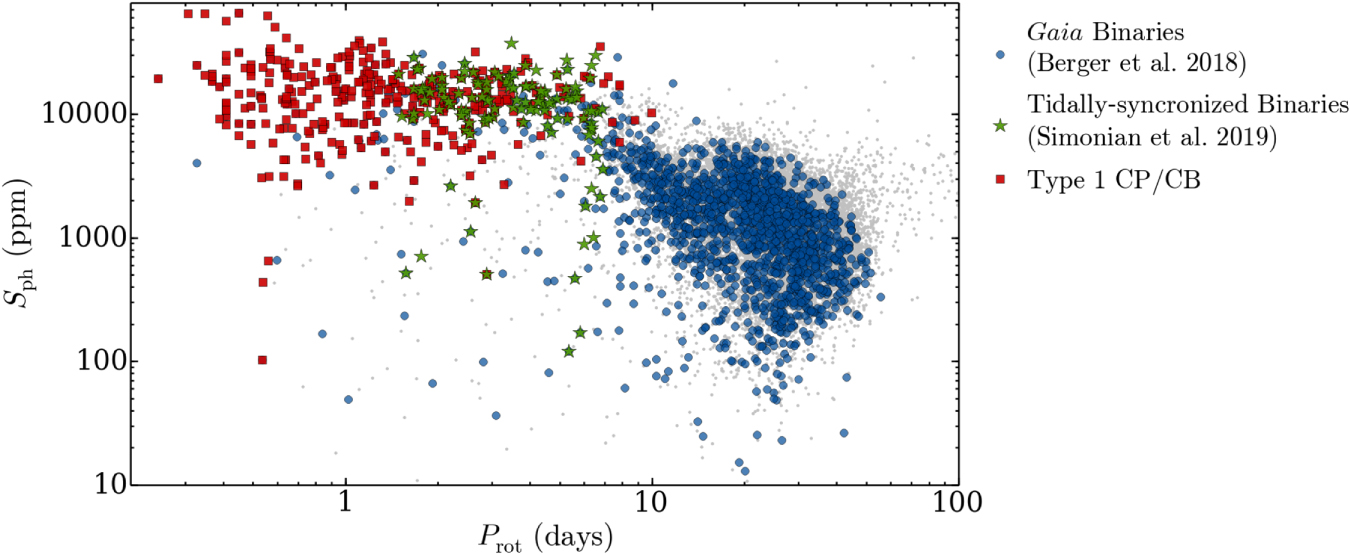
**Figure 20.** Rotation-period distributions for KEPSEISMIC (red) and PDC-MAP (black) light curves. Only the common automatically selected targets (11,131 targets) are represented.
Download figure:
Standard image High-resolution image

Surface Rotation and Photometric Activity for Kepler Targets. I. M and K Main-sequence Stars

Article metrics

Permissions

Author e-mails

Author affiliations

ORCID iDs

Dates

Abstract

1. Introduction

2. Data Preparation and Sample Selection

2.1. Data Preparation

2.2. Sample Selection

3. Surface Rotation Detection

3.1. Methodology to Retrieve Rotation Periods

3.1.1. Automatic Selection

3.1.2. Visual Check

4. Photometric Magnetic Activity Proxy

5. Results

5.1. Rotation–Mass/Temperature Relation

5.2. Photometric Activity–Mass/Temperature Relation

5.3. Photometric Activity–Rotation Relation

5.4. Comparison with McQuillan et al. (2013, 2014)

5.5. Gaia Binary Candidates

6. Summary and Conclusions

Appendix A: Rotation and Photometric Activity Index Including Potential Non-single Non-main-sequence M and K Stars

Appendix B: Comparison with the Rotation Results for PDC-MAP and KEPSEISMIC Data Sets

Footnotes

Surface Rotation and Photometric Activity for Kepler Targets. I. M and K Main-sequence Stars

Article metrics

Permissions

Share this article

Author e-mails

Author affiliations

ORCID iDs

Dates

Abstract

1. Introduction

2. Data Preparation and Sample Selection

2.1. Data Preparation

2.2. Sample Selection

3. Surface Rotation Detection

3.1. Methodology to Retrieve Rotation Periods

3.1.1. Automatic Selection

3.1.2. Visual Check

4. Photometric Magnetic Activity Proxy

5. Results

5.1. Rotation–Mass/Temperature Relation

5.2. Photometric Activity–Mass/Temperature Relation

5.3. Photometric Activity–Rotation Relation

5.4. Comparison with McQuillan et al. (2013, 2014)

5.5. Gaia Binary Candidates

6. Summary and Conclusions

Appendix A: Rotation and Photometric Activity Index Including Potential Non-single Non-main-sequence M and K Stars

Appendix B: Comparison with the Rotation Results for PDC-MAP and KEPSEISMIC Data Sets

Footnotes