


Abstract
In this study, we examine whether the First-Order Taylor Expansion (FOTE) method can be applied to steady-state plasma flow fields in space. We particularly examine whether this method (termed FOTE-V) can be used to identify the flow critical points (including both stagnation point and vortex center) and reconstruct the flow patterns around these points. Quantitatively, we test the accuracy of this method using 3D kinetic simulation data, and find the FOTE-V method can give accurate reconstruction results within an area about 2 times the size of the spacecraft tetrahedron, particularly when there are no clear nonlinear flow structures in the simulation box. With simulation data, we also reveal the ability of the FOTE-V method on reconstructing 3D flow field topology of both radial-type null and spiral-type nulls. We further test the accuracy of this method using measurements from NASA's Magnetospheric Multi-scale (MMS) mission. In a current sheet crossing event, the FOTE-V method successfully identifies the spiral-type nulls in the reconnection exhaust region. In an EDR crossing event, the FOTE-V method detects the stagnation point near the reconnection center. We find these 3D flow structures are quasi-linear at the MMS separation scale. Utilizing the continuity equation of the steady flow, we define a parameter,  , to quantify the error of this method—the smaller this parameter the better the results. This study demonstrates that the plasma flows at small scale are indeed linear, and thus the FOTE-V method can be applied to such flow fields. In particular, this method will be useful to study stagnation points and electron vortices in space plasmas.
Export citation and abstract BibTeX RIS
1. Introduction
Plasmas, consisting of electrons and ions, are indispensable elements in space and high-temperature laboratory equipment. Such matter behaves like a fluid at scales larger than the ion skin depth, similar to the water on the Earth's surface or the air in the Earth's atmosphere, and thus is termed the magnetohydrodynamic (MHD) flow. In space, such MHD flows can form various structures, such as the large-scale flow vortex at the Earth's and planetary magnetopause (termed the Kelvin–Helmholtz vortex; Otto & Fairfield 2000; Hasegawa et al. 2004), the large-scale stagnation point at the duskside plasmapause (termed the duskside bulge; Carpenter & Anderson 1992; Fu et al. 2010a, 2010b) and subsolar magnetopause (termed the nose; Pudovkin et al. 1982; Scudder 1984; Gosling et al. 1990; Phan et al. 1994), the small-scale flow vortex in the magnetosheath (termed the magnetic-hole vortex; Huang et al. 2017), and the small-scale stagnation point in the magnetic reconnection region (termed the flow-reversal point; Sonnerup & Priest 1975; Dorelli et al. 2004; Burch & Phan 2016; Chen et al. 2016).
These flow structures play very import roles in transporting and converting energies in space. For example, the Kelvin–Helmholtz vortex (large-scale vortex) can directly transport solar wind energy into the Earth's magnetosphere (Hasegawa et al. 2004; Hesegawa et al. 2009; Johnson et al. 2014) or release solar wind energy via the the reconnection process (Fu et al. 2019a, 2019b; Eriksson et al. 2016; Li et al. 2016); the duskside plasmapause bulge (large-scale stagnation point) can exchange particles between the plasmasphere and plasmatrough (Fu et al. 2010a, 2010b) and sometimes leads to the formation of plasmaspheric plumes (Goldstein et al. 2003); the magnetic-hole vortex (small-scale vortex) can lead to an energy cascade in turbulent plasmas and weakening of magnetic fields (Haynes et al. 2015); the flow-reversal point (small-scale stagnation point) in a reconnection region indicates the conversion from magnetic energy to particle energy (Burch & Phan 2016). Therefore, it is very necessary to investigate the properties of these flow structures, by using spacecraft (SC) measurements or simulations.
In theory, these four types of flow structures, as mentioned above, all correspond to critical points (or flow nulls called in some literatures; Chong et al. 1990; Jeong & Hussain 1995), where the flow velocities equal zero. Such critical points are three-dimensional (3D) in space, as shown in simulations by Roytershteyn et al. (2015) and Olshevsky et al. (2015, 2016). Investigating the 3D properties of these critical points is possible in simulations, but is very difficult in SC measurements, because typically the SC only provide a few data points at a time instant. To reveal the 3D properties of critical points in SC measurements, a method must be developed to reconstruct the flow patterns. Since the four-point measurement of plasma flow data is available in both the Cluster (Escoubet et al. 2001) and NASA's Magnetospheric Multi-scale (MMS) missions (Burch et al. 2016), a reconstruction method based on four-point data is preferable. In this study, we introduce such a method.
In fluid mechanics, flows (e.g., the Earth's atmosphere) are usually described by the Navier–Stokes and continuity equations. There have been many studies demonstrating that such flows around the critical points (including vortex and stagnation point) are 3D linear structures (e.g., Perry & Chong 1987; Chong et al. 1990; Moffatt et al. 1994; Jeong & Hussain 1995; Kida & Miura 1998; Haller 2005) and can stably exist for a long period (e.g., Hama 1967; Kline et al. 1967; Hussain 1983). In a terrestrial magnetic field system, the space plasmas can also form flows (e.g., electron flow and ion flow) that satisfy the continuity equations. We can examine whether these magnetized flows are 3D linear structures, particularly in the magnetosheath and magnetosphere, where the plasma flow may have a good linearity at a relatively small scale.
Recently, Fu et al. (2015) developed a method to reconstruct 3D linear magnetic structures in space plasmas, based on the First-Order Taylor Expansion (FOTE) of the magnetic field. Successfully, they have applied this method to study magnetic reconnection (e.g., Fu et al. 2017, 2019a, 2019b; Chen et al. 2018, 2019a, 2019c; Huang et al. 2018; Liu et al. 2018, 2019; Man et al. 2018; Wang et al. 2019) and magnetic flux ropes (Fu et al. 2016; Wang et al. 2017; Chen et al. 2019b). In this study, we extend this method (termed the FOTE-V method) to the plasma flow fields to examine whether the flows in space are 3D linear structures. We test the accuracy of this method using both the 3D kinetic simulation data and MMS measurements in a KH vortex-induced magnetopause current sheet, which is associated with a reconnection exhaust. We find that, in real space, the magnetized electron flows can be the 3D linear structures within an area about 2 times the size of the SC tetrahedron, same as the linearity of neutral fluids (Chong et al. 1990; Jeong & Hussain 1995). We therefore suggest using the FOTE-V method to study small-scale (SC separation) plasma flows in space.
We organize the paper as follows. In Section 2, the description of the FOTE-V method is presented. In Section 3, we quantitatively test the accuracy of the FOTE-V method in reconstructing flow patterns by utilizing the 3D kinetic simulation data. The ability of FOTE-V in positioning critical points (flow nulls) and reconstructing the surrounding flow fields with SC data is demonstrated in Section 4. Finally, we summarize the results in Section 5.
2. Method Description
Mathematically, a vector field at a specific time can be described as
where  are the vector coefficients and (xyz)n is the nth-order term (e.g., if n = 4, (xyz)n can be x4,
  ,
,  ...). The more higher-order terms that are considered, the more precisely the function describes the field (Liu et al. 2019). If the change of the vector fields (
 ) mainly is contributed by the first-order terms (
 ), the function can be simplified as
  , meaning that the field changes linearly around the focus point (x, y, z); in other words, it has a good linearity there. The FOTE method assumes linear changes of the magnetic field
  around an SC tetrahedron, so that the magnetic field around this tetrahedron can be expressed as
  , where
  is the magnetic field measured by the SC,
  is a 3 × 3 Jacobian matrix of the magnetic field gradient, and
  is the distance from SC to the point of interest (see Fu et al. 2015 for details). For the FOTE-V method, similarly, we assume the plasma flow velocity
  to change linearly around the SC tetrahedron, and express the flow velocity around this tetrahedron as
  , where
  is the flow velocity measured by the SC,
  is a 3 × 3 Jacobian matrix of the velocity gradient, and
  is the distance from SC to the point of interest. With four-point measurements, the velocity
  and the Jacobian matrix
  can be easily obtained, and thus the position of critical point (flow null)
  can be resolved by requiring
  . In the FOTE method, the eigenvalues and eigenvectors of the Jacobian matrix
  are used to identify magnetic-null types (A, B, As, Bs, X, O) and establish the coordinates for magnetic-topology reconstruction (see Fu et al. 2015 for details). Similarly, in the FOTE-V method, the eigenvalues and eigenvectors of the Jacobian matrix
  can be used to identify the types of critical points (flow nulls) and establish the coordinates for flow-pattern reconstruction, as discussed by Chong et al. (1990). If all the eigenvalues are real, the null is of radial type (node), which includes A type and B type. If one eigenvalue is real while the two others are conjugate complex, the null is of spiral type, which includes As type and Bs type (Chong et al. 1990; Burch et al. 2016). They can, however, degenerate into 2D structures (X type and O type) when one of the eigenvalues is much smaller than the other two. Once the Jacobin matrix
  is obtained with four-point measurements, we can trace the flow streamlines around the null using the FOTE-V formula
  and reconstruct the flow field topology that reveals both the direction and magnitude of the vector field.
In this study, we mainly focus on investigating the suitability of employing the FOTE-V method as a mathematical tool to analyze the plasma electron flow fields in simulation and real space, leaving the detailed physics behind the different type nulls to our future studies. To judge the accuracy of the FOTE method, Fu et al. (2015) use the nondivergence condition of the magnetic field,  , because this condition should be theoretically satisfied. Similarly, to judge the accuracy of the FOTE-V method, we introduce the continuity equation
  , where n is the plasma number density and
  is the flow velocity. Considering a steady-state plasma (
 ), which exists widely in space such as the solar wind and magnetosheath, the continuity equation becomes
  . In this sense, we can use the value of
  to judge the accuracy of the FOTE-V method in steady-state plasmas. We normalize this value using the curl of the flow flux,
  , to get a dimensionless parameter
  , similar as that done in the FOTE method. Following Fu et al. (2015), we treat the FOTE-V results as unreliable if α is greater than 40%.
3. Benchmark Test and Topology Reconstruction Using Simulation Data
In this section, we test the accuracy of FOTE-V in reconstructing 3D electron flow patterns. The electron flow data we investigate are taken from the 3D particle-in-cell (PIC) simulation of a reconnection event by Olshevsky et al. (2015, 2016). Specifically, we compare the flow velocity vector resolved by FOTE-V ( ) with that from simulation (
 ), and normalize the magnitude of their difference (
 ) using the median value of the simulation velocity (
 ) to get a dimensionless parameter (
 ), which is defined as the normalized error of the FOTE-V method. Since any small difference (
 ) can result in big relative errors when the flow velocity is approaching zero, such a normalized error is more reasonable than the relative error.
We consider two snapshots in the simulation run (see Olshevsky et al. 2015 for details): (1) early stage (Ωcit = 3.6) and (2) later stage (Ωcit = 36). The magnitude of electron flow velocities at these two snapshots is shown in Figures 1(a) and (b). As can be seen, at Ωcit = 3.6 (Figure 1(a)), the electron flow field is less chaotic, showing only large-scale flow structures in the simulation box; while at Ωcit = 36 (Figure 1(b)), the electron flow field becomes very chaotic and many small-scale flow structures appear in the simulation box. The whole simulation box (Figures 1(a) and (b)) has size  and consists of 250 × 250 × 250 cubes (Olshevsky et al. 2015), and thus the resolution of simulation is 0.05di or 1 point (hereafter pts). We only test the FOTE-V method in a small box with a size of
  (
( cubes), because this method aims to study flow fields in a limited range around the SC. The flow fields in the two boxes of interest are shown in Figures 1(c) and (d), with the first box (early stage) centered at (225, 168, 218) pts and the second box (later stage) centered at (105, 26, 180) pts. We examine the continuous equation by calculating the
  term at each point in the tested boxes (
 =
= 
 , where i, j, k are the number of grid points), and find the magnitude of
  is significantly smaller than the magnitude of
  , indicating that the flow field in the first box (Figure 1(c)) tend to be steady
  . Meanwhile, in the second box (Figure 1(d)), the flow field is more chaotic than in the first one (Figure 1(c)).
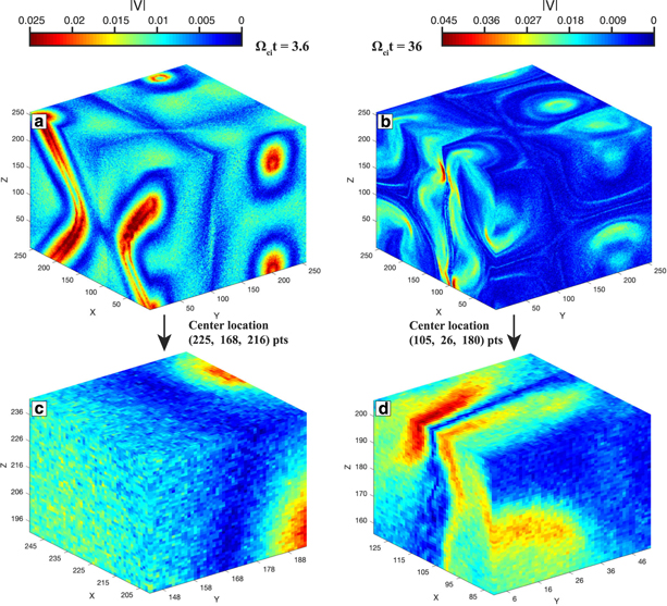
Figure 1. Snapshots from the PIC simulation (Olshevsky et al. 2015, 2016) corresponding to the evolution stage Ωcit = 3.6 and Ωcit = 36, colored with flow field magnitude. (a), (b) The overall snapshot of the less-turbulent flow at Ωcit = 3.6 and turbulent flow at Ωcit = 36. (c), (d) The snapshot of the flow fields in two small boxes of interest, centered at (225, 168, 216) pts in (a) and (105, 26, 180) pts in (b), respectively.
Download figure:
Standard image High-resolution imageThe comparison between the reconstruction results and simulation results in these two boxes of interest is presented in Figures 2 and 3. Specifically, Figures 2(a) and 3(a) show the electron flow fields in the 3D simulation box; Figures 1(b)–(d) and Figures 3(b)–(d) show three cuts of the simulation results in the XY plane (Z = 218 pts for Figure 2 and Z = 180 pts for Figure 3), XZ plane (Y = 168 pts for Figure 2 and Y = 26 pts for Figure 3), and YZ plane (X = 225 pts for Figure 2 and X = 105 pts for Figure 3); Figures 2(e)–(g) and Figures 3(e)–(g) show the reconstruction results from the FOTE-V method in these planes; and Figures 2(h)–(j) and Figures 3(h)–(j) show the normalized error of the FOTE-V reconstruction in these planes. In both Figures 2 and 3, the reconstruction is based on a tetrahedron with a size of 0.7di (14 pts; see the white dots in Figures 2(e)–(g) and Figures 3(e)–(g)). Approximately, such a size is comparable to the separation of the MMS mission (Burch et al. 2016). For the first case (Ωcit = 3.6; Figure 2), we have examined the flow pattern in the simulation box ( cubes), and we find it belongs to a stagnation point (see Figure 5). The magnitude of the surrounding flow (Figures 2(b)–(d)) increases with the distance, from nearly zero at the center (dark blue) to 0.025 (red) at the edge. The virtual tetrahedron covers a region in which the flow magnitude changes from nearly zero to 0.01 (cyan). Considering the size of the tetrahedron is nearly one-quarter of the size of the simulation domain, the increment of flow magnitude is proportional to the distance from the center, indicating the flow field is quite linear. The FOTE-V reconstruction (Figures 2(e)–(g)) can generally reproduce the flow features in simulations (Figures 2(b)–(d)). The normalized error (Figures 2(h)–(j)) is generally smaller than 40% in the reconstruction region, and the big error only appears at the edge of the box (see Figures 2(i)–(j)). This test (Figure 2) means that the FOTE-V method works well in the box of interest, and the flow patterns in this box (about 2 times the tetrahedron size) can be accurately reconstructed. For the second case (Ωcit = 36; Figure 3), there exist some large-velocity stripes (with a magnitude of 0.04) in the simulation domain (Figures 3(b)–(d)), clearly indicating the "nonlinearity." The virtual tetrahedron covers a region where the flow magnitude gradually changes from 0.01 (dark blue) to 0.03 (light yellow), which is comparable to that of the whole simulation domain. We find that the FOTE-V reconstruction (Figures 3(e)–(g)) can only reproduce the main feature of the chaotic flow structure in the simulation box (the flow magnitude changes from dark blue to light yellow along nearly the same direction) but fails to reproduce the nonlinear stripe structures (see Figures 3(b)–(d)). The normalized error (Figures 3(h)–(j)) is roughly smaller than 40% except in the nonlinear stripe regions, where the normalized error is over 80% (see Figures 3(h)–(j)). This indicates that the accuracy of the FOTE-V result is mainly determined by the flow fields' linearity, rather than whether the flows are nearly stagnant. However, it does not mean that FOTE-V method cannot be used to study the nonlinear space plasmas at all. In this simulation test, though FOTE-V method fails to capture the secondary nonlinear stripes, it reveals the large-scale features of the flow field (e.g., the gradient orientation and the range of velocity magnitude). In addition, even the nonlinear stripes can appear to have a quasi-linear structure if the observation scale is relatively small (e.g., if we reduce the scale of simulation box to
  cubes, then the nonlinear stripes around the lower left corner of the simulation slice in Figure 3(a) can roughly seem to be quasi-linear). Therefore, when we apply the FOTE-V method on space plasmas, the linearity of the flow fields should be carefully analyzed at the observation scale. For this purpose, we introduce a linearity test method in Section 4.

Figure 2. Testing the accuracy of FOTE-V method in reconstructing the flow field magnitude in less-chaotic (quasi-linear) flow. The flow field around (225, 168, 216) pts at Ωcit = 3.6 is considered. (a) The snapshot of the tested flow field, same as Figure 1(c). (b)–(d) Flow field magnitude from simulations and (e)–(g) the FOTE-V method. (h)–(j) Normalized error of FOTE-V in reconstructing flow patterns. The white dots are the points based on which the FOTE-V method performed. The separation of the point is 14 pts about 0.7 di, which is comparable to the flow field structure. Only the (a)–(g) flow field magnitudes and (h)–(j) normalized error at cuts Z = 216 pts (b), (e), and (h), Y = 168 pts (c), (f), and (i), and X = 225 pts (d), (g), and (j) are shown.
Download figure:
Standard image High-resolution image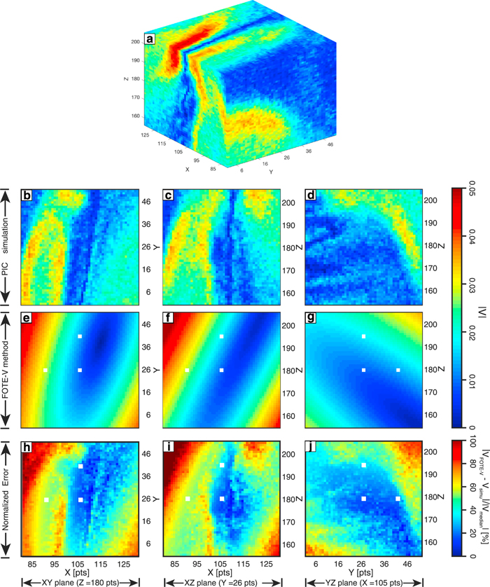
Figure 3. Testing the accuracy of the FOTE-V method in reconstructing the flow field magnitude in chaotic flow (with nonlinear stripes), in the same format as in Figure 2, except that the chaotic flow field around (105, 26, 180) pts at Ωcit = 36 is considered.
Download figure:
Standard image High-resolution imageSince the SC tetrahedron has a variable size in SC measurements (e.g., MMS/Cluster) and it can encounter the flow nulls from any direction, testing the method with a fixed position and separation is insufficient to illustrate its capacity on finding actual flow nulls with in situ SC data. Thus, we test the FOTE-V method with different positions and scales of the virtual tetrahedron through the PIC simulation domain, and present the result in Figure 4. In order to make a comparison with the former test, the simulation domain is same as the one in Figure 2. To investigate the influence from SC position, we set the virtual tetrahedron in different regions of the simulation box and reconstruct the flow field with the FOTE-V method in Figures 4(b) and (c) (the tetrahedron is moved 10 pts along the X direction and 5pts along the Z direction, respectively). To investigate the influence from SC separation, we test the FOTE-V method using different tetrahedron scales in Figure 4(f) (10 pts ∼ 0.5di) and Figure 4(g) (7 pts ∼ 0.35di). We see that the FOTE-V method based on different tetrahedron gives a similar result as the simulation (Figure 4(a)), and the normalized error is generally smaller than 40% in a box about 2 times the tetrahedron size (Figures 4(d), (e), (h), and (i)). Like the FOTE method, the FOTE-V method can reconstruct the flow field from any direction of the null (Figures 4(b) and (c)). If the flow field is not involved with nonlinear stripes, the size of a reliable region is mainly due to the scale of the virtual tetrahedron. As the spacing reduced, the reliable region also shrank (Figures 4(h) and (i)). These six tests (Figures 2–4) indicate that, at the MMS observation scale, the FOTE-V method can give accurate reconstruction results within an area about 2 times the size of SC tetrahedron, if there are no clear nonlinear structures in the simulation box. The FOTE-V method is capable of solving actual flow nulls with complex in situ SC measurements.

Figure 4. Testing the accuracy of the FOTE-V method in the same format as Figure 2, except that in (b), (d) and (c), (e) the 14 pts size virtual tetrahedron is placed in different regions of the simulation box. In (f), (h) and (g), (i), the scales of the virtual tetrahedron are 10 pts (0.5di) and 7 pts (0.35di).
Download figure:
Standard image High-resolution imageTo further illustrate the ability of the FOTE-V method to impact the analysis of 3D flow velocity fields, we identify the streamline topology of both the radial-type flow null and spiral-type flow null with the simulation data at early stage. We select the simulation box centered at (225, 168, 218) pts, where the shearing flow components converge and form a radial-type flow null/critical point (Figure 5), and the simulation box centered at (38, 230, 166) pts, where the electron flow rolls up in the X–Y plane and forms a spiral-type flow null/critical point (Figure 6). The 3D view of the simulation streamlines is shown in Figures 5(a) and 6(a), with the color denoting the magnitude of the velocity vector and the small red arrows denoting the flow direction. Figures 5(b) and 6(b) are the projection along the Z direction. The feature of the shearing flows and null center can be easily found in Figure 5(b), while the streamlines are rotated around the null center in Figure 6(b), clearly showing the difference between radial-type null and spiral-type null. To avoid the visual influence from the overlapping lines, we also present the 2D flow pattern at Z = 198 pts for the radial-type null and at Z = 166 pts for the spiral-type null in Figures 5(c) and 6(c), in which the blue lines represent the streamlines and red arrows denote their direction. It is clear that an "X" shape exists in the 2D flow pattern in Figure 5(c), indicating the null/critical point in the simulation box is of radial type. Meanwhile, the 2D flow pattern in Figure 6(c) presents rotating "O" shape streamlines, which is a typical feature of spiral-type null. Using the FOTE-V method, we trace and inverse trace the streamlines around the null/critical point to obtain the streamline topology. The reconstructed streamline topologies are shown in Figures 5(d)–(f) and Figures 6(d)–(f), respectively, and organized in the same way as in Figures 5(a)–(c) and Figures 6(a)–(c) except that the black squares are added to show the points based on which the FOTE-V method performed. Compared with the simulations, we find that the FOTE-V method can well reveal both the magnitude and direction of the electron flow field (Figures 5(d)–(f) and Figures 6(d)–(f)). Moreover, the reconstructed 2D streamline topology also has an "X" shape in Figure 5(f) and an "O" shape in Figure 6(f), which are well consistent with the simulations. The good consistency between the reconstructed streamlines and simulations, together with the promising benchmark tests, suggests that the linearity assumption is reasonable for the electron flow fields at the MMS observation scale, and thus the FOTE-V method is a potential tool to study the flow fields in space.

Figure 5. Streamlined topology of the simulation radial-type null (the flow fields in Figure 2) and the corresponding reconstruction from the FOTE-V method. (a) The 3D view of the simulation streamlines and (b) the projection along the Z direction, with the color denoting the magnitude of the local velocity and small red arrows denting the flow direction. (c) The 2D streamline in the X–Y plane at Z = 198 pts, in which we ignore the Z component of the flow field. (d)–(f) The FOTE-V reconstruction of the flow field structures, organized in the same format as (a)–(c). The black squares are the location of the virtual satellites based on which the FOTE-V method operated.
Download figure:
Standard image High-resolution image
Figure 6. Streamlined topology of the simulation spiral-type null (centered at (38, 230, 166) pts in the early stage simulation box; Figure 1(a)) and the corresponding reconstruction from the FOTE-V method. (a) The 3D view of the simulation streamlines and (b) the projection along the Z direction, with the color denoting the magnitude of the local velocity and small red arrows denting the flow direction. (c) The 2D streamline in the X–Y plane at Z = 166 pts, in which we ignore the Z component of the flow field. (d)–(f) The FOTE-V reconstruction of the flow field structures, organized in the same format as (a)–(c). The black squares are the location of the virtual satellites based on which the FOTE-V method operated.
Download figure:
Standard image High-resolution image4. Application to SC Data
In this section, we demonstrate that the steady flows in space are indeed linear at small scale, and thus we can apply the FOTE-V method to reconstruct these flows. The data we used are from the MMS mission (Burch et al. 2016). Specifically, the electron flow data, with a resolution of 30 ms, are from the Fast Plasma Investigation (FPI) suite (Pollock et al. 2016); the magnetic field data, with a sampling rate of 128 Hz, are from the Fluxgate Magnetometer (Russell et al. 2014). The SC separations are variable from 10 to 160 km, depending on the phase of the mission. Respectively, we consider two representative magnetic reconnection events measured by MMS at the dayside magnetopause.
The first event is measured by MMS on 2015 September 8. It is a magnetic reconnection event associated with large-scale K-H vortices (see Eriksson et al. 2016 and Li et al. 2016 for details). However, we only focus on small-scale critical points within the reconnection exhaust region since the MMS observation scale is incomparable to the large-scale K-H vortex. Figures 7(a)–(i) are the overview of this event, in which the MMS measured the reconnection exhaust region close to a K-H vortex-induced current sheet. The measurements are presented in the LMN coordinates given by Eriksson et al. (2016), in which L denotes the maximum variance direction of magnetic field during the current sheet crossing, N is normal to the boundary and away from the Earth, and M completes the right-hand coordinates system, denoting the guide field direction. Relative to the GSE coordinates, L = [−0.171, 0.984, −0.057], M = [0.253, 0.100, 0.962], and N = [0.962, 0.160, −0.266]. As can be seen, during the whole interval, MMS3 and MMS4 generally measured positive BL components and small plasma densities, while MMS1 and MMS2 measured a reversal of BL and an increase of plasma densities (Figures 7(a) and (d)), meaning that the four MMS SC were generally in the magnetosphere except for an excursion of MMS1 and MMS2 to the magnetosheath. The L component of ion velocity measured at MMS1 climbed from ∼+200 km s−1 (background) to a peak of +410 km s−1 (fast exhaust flow) during the same interval (Figure 7(b)), indicating that the MMS tetrahedron is located in the reconnection exhaust region where the ions and electrons flowing away from the reconnection X-line. In this event, the FPI instrument had different swept energy for the even and odd sampling cycles, specifically, 11 eV–24.4 keV for the Even Sweep Cycle (ESC) and 12.4 eV–27.6 keV for the Odd Sweep Cycle (OSC; see Pollock et al. 2016 for details). Since there are fewer electrons with higher energy in the solar wind, the FPI suite would measure a smaller electron flux in the OSC (Figure 7(c)), which results in smaller plasma density and velocity (not shown). To remove this artificial effect caused by the working mode of FPI, we consider only the ESC data set (notice that the electrons have energies primarily below 1 keV, and thus the lower energy/charge sampling cycle can provide more accurate measurements), and substitute the OSC data set using the average value of the nearby ESC data. The calibrated plasma density and omnidirectional flux are shown in Figures 7(d) and (e), respectively. As can be seen, the artificial fluctuation has been removed, meaning that such a calibration can well reduce the errors caused by instruments. Considering the absence of photoelectrons in this event and the coverage of most electrons by the FPI measurement range (Figure 7(e)), such calibrated data are readily reliable. Thus, we can apply the FOTE-V method to these data. Since the measurement at different SC is not synchronous (Figures 7(k)–(n) and (q)–(t)), we also resample the raw data to a higher resolution (128 samples per second) to obtain a synchronous data set of four SC. The calibrated omnidirectional flux and flow velocity at MMS1 are shown in Figures 7(e) and (f).

Figure 7. Examination of the FOTE-V method in a well-studied K-H vortex event at the dayside magnetopause on 2015 September 8. Specifically, they are (a) the L component of magnetic field; (b) the ion velocity measured at MMS1; (c) and (e) the raw and calibrated omnidirectional differential energy fluxes at MMS1; (d) the calibrated electron number density; (f) and (g) the calibrated electron velocity at MMS1, with and without the background flow velocity Veb = [235, 30, −131] km s−1 (estimated by the mean value of the electron velocities during the whole interval); (h) the distance from the critical point to each MMS SC as well as their type resolved from the FOTE-V method; and (i) the dimensionless parameter,  , for quantifying the uncertainty of the FOTE-V method. Two black vertical lines mark the most reliable critical point at 11:01:18.75 UT (of radial type) and the closest critical point at 11:01:19.11 UT (of spiral type), at which the surrounding flow fields' linearity (11:01:18.68–11:01:18.82 UT and 11:01:19.07–11:01:19.17 UT, shaded areas) are examined in Figures 6(j)–(o) and (p)–(u), respectively. Specifically, they are (j) and (p) the distance change of four MMS SC relative to their locations at central points; (k)–(n) and (q)–(t) the flow fields (without the background flow velocity) observed by the four MMS SC (solid lines) and reconstructed by the FOTE-V method (dashed lines), with blue stars denoting the sampling time of the raw 30 ms electron velocity data; and (o) and (u) the average error between the reconstructed and observed flow velocities,
  . All components are shown in given LMN coordinates (Eriksson et al. 2016), relative to the GSE coordinates, L = [−0.171, 0.984, −0.057], M = [0.253, 0.100, 0.962], and N = [0.962, 0.160, −0.266].
Download figure:
Standard image High-resolution imageSimilar to the critical points in the turbulent solar wind, the critical points generated by the shearing between reconnection exhaust flow and the background plasmas is also comoving with the "background flow" (e.g., the center of a vortex, the stagnation point formed by two shearing flows are not static, probably moving with a specific speed). Thus, to resolve a flow null (vortex center) in the current sheet region where it is associated with the exhaust flow, we must subtract the background flow velocity as well. The background flow velocity  is estimated with the average of the mean velocity of the electron flow measured at the four MMS SC (
 ). In this event, the background velocity is about
  = [235, 30, −131] km s−1 (calculated over the 2 s overview interval), which is nearly same as the background ion flow (Figure 7(b)). The null-SC distance as well as null type resolved from the FOTE-V method are shown in Figure 7(h). As can be seen from the panel, the FOTE-V method successfully detects the critical points with the null-SC separation smaller than 100 km. The majority of the nulls are of spiral type (vortex center), and the radial-type nulls tend to occur in two adjacent spiral nulls. Such a result is quite consistent with the scenario that a succession of small-scale vortices rolled up at the edge of the fast exhaust flow and the stagnation point (radial null) thus formed at the interface of two developing vortices. This scenario is also quite consistent with the recent simulations by Che & Zank (2020), where the electron-scale vortices can be triggered by the electron velocity difference within the reconnection current sheet, suggesting that the FOTE-V result is reasonable. Figure 7(i) examines the continuity equation of the steady flow, which can verify the accuracy of the flow-velocity measurements: if the electron velocities are accurately measured and simultaneously the plasma densities are temporally stationary, the continuity equation should be strictly satisfied with
  . As mentioned above, we treat the velocity measurements as reliable and then apply the FOTE-V method if α < 40% (horizontal dashed line). In this event, we notice that α is generally below 40% during the whole interval, meaning that the application of FOTE-V is feasible.
Due to the limitation of four-point measurements, we cannot directly examine the accuracy of the FOTE-V method by comparing the reconstruction with the observation. Since this method is based on the linear assumption of flow fields, there is no doubt that the FOTE-V method can work well if the flows have good linearity at the scale of MMS separation. To address this issue, we assume the critical-point structure has no temporal evolution ( ) to obtain an SC trajectory, and then we are able to test the structure's linearity by comparing the reconstruction results with the observations along this trajectory. We consider two different types of flow nulls around 11:01:18.75 UT (radial null) and 11:01:19.11 UT (spiral null) as the example (see the vertical gray shade in Figure 7). During the first encounter from 11:01:18.68 to 11:01:18.82 UT, the critical point was in a very steady state plasma with a distance change from 60 to 100 km. As for the second encounter from 11:01:19.07 to 11:01:19.17 UT, the critical point was first approaching the MMS tetrahedron then flowing away, with the closest distance about 15 km (Figure 7(g)). The observational electron flow velocities during these two encounters are shown in Figures 7(k)–(n) and (q)–(t), respectively, with the red solid line denoting the L component, the green solid line the M component, the blue solid line the N component, and the black solid line the total strength. Since the flow structure is temporally stationary (
 ), the change of the observational electron flow velocities (Figures 7(k)–(n) and (q)–(t), solid lines) is only due to the movement of MMS relative to the flow structure, and we can solve the MMS trajectory (
 ) by integrating the distance change at each sample point (
 ). Here we trace/inverse trace the MMS trajectory (
 ) from 11:01:18.75 UT and 11:01:19.11 UT (marked with the vertical dashed line in Figure 7), and the distance change (
 ) of four MMS SC are shown in Figures 7(j) and (p). Utilizing the measured flow velocity (
 ) and the gradient (
 ) at the two central points, we reconstruct the flow velocity along the SC trajectory (
 ) and show the results in Figures 7(j)–(m) and (p)–(s) (the dashed lines). We find that the reconstructed flow velocities at the four MMS SC agree with the observations very well along the inferred trajectory, with the average error
  smaller than 20% (Figures 7(o) and (u)). This means that the flow fields around the critical points (flow nulls) are very linear in the magnetopause current sheet, and thus the FOTE-V method will be accurate in reconstructing the flow patterns around these points.
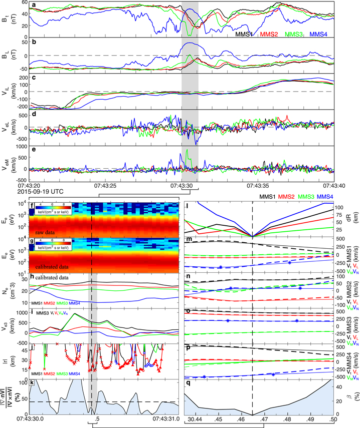
The second event is a well-studied reconnection event measured on 2015 September 19 from 07:43:20 UT to 07:43:40 UT, during which the MMS tetrahedron crossed a magnetopause reconnection region from southward to northward (see Chen et al. 2016 and Wang et al. 2019 for details). Figures 8(a)–(e) are the 20 s overview of the event, in which the measurements are presented in LMN coordinates given by Chen et al. (2016). Relative to the GSE coordinates, L = [0.0892, 0.2309, 0.9689], M = [0.7958, −0.6015, 0.0701], and N = [0.5990, 0.7648, −0.2374]. During the whole interval, the four MMS SC generally measured the negative BL component dominating the total magnetic strength Bt, except MMS4 measured a reversal of BL (Figures 8(a) and (b)), indicating that the MMS tetrahedron was primarily in the magnetosheath, except that MMS4 had a brief excursion to the magnetosphere. All four SC measured ion-flow reversal (Figure 8(c); from ViL ≈ −250 km s−1 to ViL ≈ 180 km s−1), while only MMS3 and MMS4 detected the reconnection electron jet (Figure 8(e); VeM ≈ 900 km s−1). These features indicate that the MMS tetrahedron crossed the reconnection region from southward to northward, with MMS3 and MMS4 closer to the EDR—the reconnection center. During the time interval from 07:43:30 UT to 07:43:31UT, while MMS3 and MMS4 measured the reversal of the VeL component (at the level of VeL ≈ ± 300 km s−1), VeL at MMS1 and MMS2 is close to zero, suggesting that the MMS tetrahedron might be close to the critical points/flow nulls. Thus, we apply the FOTE-V method to the MMS measurements during this interval (shaded area), and the result is presented in Figures 8(f)–(k).
Figure 8. Examination of the FOTE-V method in a well-studied EDR crossing event at the dayside magnetopause on 2015 September 19. The data are shown in given LMN coordinates (Chen et al. 2016), relative to the GSE coordinates, L = [0.0892 0.2309 0.9689], M = [0.7958–0.6015 0.0701], N = [0.5990 0.7648–0.2374]. The upper panel is a 20 s overview of the event. Specifically, they are (a) the magnitude of the magnetic field, (b) the L component of the magnetic field, (c) the L component of the ion-flow velocity, (d) the L component of the electron flow velocity, and (e) the M component of the electron flow velocity. The shaded area marks the time interval from 07:43:30.00 UT to 07:43:31.10 UT, during which the FOTE-V method is applied to the calibrated electron flow velocity data. The result is shown in the lower left panels, specifically, they are (f) and (g) raw and calibrated omnidirectional differential energy fluxes at MMS3, (h) the calibrated electron number density, (i) the calibrated electron velocity at MMS3, (j) the null-SC distance together with the null type resolved from the FOTE-V method, and (k) the dimensionless error parameter,  . The dashed vertical line marks the most reliable and closed critical point at 11:01:18.75 UT (of X type), at which the surrounding flow field's linearity (09:43:30.435–09:43:30.50 UT, shaded area) is examined in (l)–(q) (organized in the same format as the linear test panels in Figure 7).
Download figure:
Standard image High-resolution image
In this event, the FPI instrument also had different swept energy for the even and odd sampling cycles (Pollock et al. 2016); thus we calibrate the plasma data using the same method as in the first event (Figures 8(f) and (g)). Figure 8(h) is the calibrated electron number density at the four MMS SC, and Figure 8(i) is the calibrated electron flow velocity at MMS3. Since the background flow velocity is close to zero during this interval (Figure 8(c)), we did not take it into account when identifying the critical points/flow nulls with the FOTE-V method. The results of the FOTE-V method (both the null-SC distance and the null type) are presented in Figure 8(j). As can be seen from the figure, the FOTE-V method finds the X-type flow nulls (quasi-2D radial nulls) around the peak of the fast electron jet, while some small-scale spiral nulls (vortex center) are at the edge of the jet. Such a result is quite consistent with the reconnection picture, since the speed of the electron inflow is significantly smaller than that of the outflow and the reconnection jet and the reconnection stagnation point tends to show the 2D feature. Meanwhile, at the edge of the fast reconnection jet, small-scale vortex can be formed due to the velocity shear between the jet electrons and the background electrons.
Similar to the first event, we examine the linearity of the flow field around the stagnation point at 07:43:30.465 UT (vertical line) since it has a small error parameter (Figure 8(k)). Specifically, we calculate the SC trajectory (Figure 8(l)) during 09:43:30.43 UT–09:43:30.50 UT (see the vertical gray shaded region in Figures 8(f)–(k)) by assuming the flow structure is temporally stationary. We find that the reconstructed flow velocities at the four MMS SC (dashed lines in Figures 8(m)–(p)) agree with the observations (solid lines) very well along the inferred trajectory, with the average error  generally smaller than 20% (Figure 8(q)). This means that the flow field around the critical point at 07:43:30.465 UT is very linear, and thus the FOTE-V method is accurate in positioning these points and reconstructing the surrounding flow fields. With these two MMS events, the existence of 3D linear flow structures is confirmed in real space. Thus, there is no doubt that the FOTE-V method can serve as a mathematical tool on future studies associated with space plasma flow.
5. Summary and Discussion
In this study, we extend the FOTE method, which was developed for magnetic-null identification and magnetic-topology reconstruction in previous studies (Fu et al. 2015), to three-dimensional plasma flow fields, in order to analyze flow properties in space plasmas. We examine whether this method (termed FOTE-V) can be used to position flow nulls and reconstruct flow patterns around the null. Using data from the 3D kinetic simulation, we quantitatively test the accuracy of FOTE-V in reconstructing the flow patterns. Two evolution stages in the simulation run (Ωcit = 3.6 and Ωcit = 36) are tested. From the test, we find that the FOTE-V method can give accurate reconstruction results within an area about 2 times the size of SC tetrahedron, if there are no clear nonlinear structures in the simulation box.
We define a parameter  , by utilizing the continuity equation of the steady flow, to quantify the accuracy of the FOTE-V method. The smaller this parameter, the more accurate the results. By examining MMS measurements in two well-studied reconnection events, we find that the flow fields have good linearity around different types of critical points (flow nulls) at the scale of MMS separation. Thus, we can employ the FOTE-V method to position critical points and reconstruct the surrounding flow patterns, by using the four-point MMS measurements. We assume the flow-null structure to be temporally stationary to obtain an SC trajectory, and then we are able to compare the reconstruction results with the observations along this trajectory. We find that in the current sheet crossing event the reconstruction and observation are well consistent around different types of critical points, with the error
  smaller than 20%. This means that the electron flow field in real space can have good linearity at small scale, and thus the FOTE-V method can be applied to such kinds of flows. Using this approach, we can also estimate the error of the FOTE-V method. Considering these two parameters (
 and
and  ) together, the error of the FOTE-V method can be well estimated.
Notice that, to examine the accuracy of the reconstruction in SC measurements, we must assume the flow structure to be stationary. However, this does not mean that the FOTE-V method can only resolve a stationary flow structure. In fact, the FOTE-V method is only based on four-point measurements of electron flows, and thus it can resolve temporal evolution of a flow structure, like the FOTE method (Fu et al. 2015).
This method will be useful to study the four types of flow nulls (critical points) in space, including the Kelvin–Helmholtz vortex at the magnetosphere (large-scale vortex), the duskside plasmapause bulge (large-scale stagnation point), the magnetic-hole vortex in the magnetosheath (small-scale vortex), and the flow-reversal point in the reconnection region (small-scale stagnation point). Since the linear FOTE-V method can give accurate results within an area about 2 times the size of SC tetrahedron only when the flows structures have good linearity at observation scale, it is better to use some large-scale observation techniques to study the large-scale flow nulls with the FOTE-V method. In this study, we only focus on the flow-null search at the MMS observation scale. We will discuss the whole null-type identification (vortex or stagnation point, small scale, and large scale) and flow-pattern reconstruction in our future work.
We thank the MMS Science Data Center (https://lasp.colorado.edu/mms/sdc/public/) for providing the data for this study. This work was supported by NSFC grants 41874188 and 41821003.