


Abstract
In this study, we extend the prior interstellar pickup ion (PUI) observations from the Solar Wind Around Pluto (SWAP) instrument on New Horizons out to nearly 47 au—essentially halfway to the termination shock in the upwind direction. We also provide significantly improved analyses of these and prior observations, including incorporating a cooling index, α, to characterize the nonadiabatic heating of PUI distributions. We find that the vast majority (93.6%) of all distributions show additional heating above adiabatic cooling. Speed jumps indicate compressional waves and shocks with associated enhancements in core solar wind and PUI densities and temperatures. Interestingly, additional heating of the PUIs as indicated by a peak in the cooling index follows the jumps by about a week. We characterize nearly continuous solar wind and H+ PUI data over ∼22–47 au, producing radial gradients, "fiducial" values at 45 au—halfway to the nominal upstream termination shock—for direct comparison to models, and extrapolated values at the shock. These termination shock values are nPUI = (4.1 ± 0.6) × 10−4 cm−3, TPUI = (5.0 ± 0.4) × 106 K, PPUI = 30 ± 4 fPa, α = 2.9 ± 0.2, nPUI/nTotal = 0.24 ± 0.02, TPUI/TSW = 716 ± 124, PPUI/PSW = 173 ± 32, PPUI/PSW − Dyn = 0.14 ± 0.01. The PUI thermal pressure exceeds by more than an order of magnitude the thermal solar wind and magnetic pressures in the outer heliosphere. SWAP provides the first and only direct observations of interstellar PUIs in the outer heliosphere, which are critical for both inferring the plasma conditions at the termination shock and understanding PUI-mediated shocks in general. This study examines these observations and serves as the citable reference for these critical data.
Export citation and abstract BibTeX RIS

Original content from this work may be used under the terms of the Creative Commons Attribution 4.0 licence. Any further distribution of this work must maintain attribution to the author(s) and the title of the work, journal citation and DOI.
1. Introduction
The Sun continuously emits solar wind that travels supersonically outward in all directions. This plasma fills interplanetary space and inflates a bubble—our heliosphere—in the surrounding very local interstellar medium (VLISM). The solar wind plasma is magnetized and thus carries the interplanetary magnetic field (IMF) out with it. Because of the rotation of the Sun, the IMF forms an Archimedean spiral that becomes, on average, increasingly transverse with distance. The solar wind is variable, with both transient structures and faster and slower streams. Parcels of faster plasma overtake slower ones, interacting with them and forming compressions both ahead of fast transients and in corotating interaction regions (CIRs); some compressions ultimately steepen into traveling interplanetary shocks.
Interstellar neutral (ISN) atoms from the VLISM are not affected by the solar wind plasma or IMF and propagate into the heliosphere with a relative velocity to the Sun of ∼25.4 km s−1 (e.g., McComas et al. 2015). When such neutrals are ionized, they immediately begin to gyrate, owing to the motional electric field of the moving IMF, and are thus incorporated into the solar wind plasma and carried out by its flow. These interstellar pickup ions (PUIs) have a velocity distribution in the solar frame that spans from roughly zero (their initial neutral flow speed) to twice the solar wind speed, depending on their pitch angle and the phase of their gyromotion. PUIs rapidly scatter in angle, forming a nearly isotropic shell in velocity space, and then much more slowly cool, progressively filling in the shells closer and closer to the solar wind speed over time. Simultaneously, new interstellar neutrals are ionized, becoming PUIs that join the distribution by adding to its outermost shell.
Interstellar PUIs were anticipated theoretically, and Vasyliunas & Siscoe (1976) developed a model for the distribution including ionization of the incoming neutrals, instantaneous scattering into an isotropic distribution in the solar wind frame, convection, and adiabatic cooling. Their model with further reconciliation (McComas et al. 2017b) can be expressed in the solar wind frame as
where r is the distance from the Sun, w = v/vb is the ratio of the PUI speed (v) to the injection speed (vb), b0 is the ionization rate normalized to r0 = 1 au, usw is the solar wind bulk speed in the solar frame, θ is the angle between radial and the ISN hydrogen inflow direction, nH,TS is the density of the ISN hydrogen at the upwind termination shock, λ is the ISN hydrogen ionization cavity size, and Θ is the Heaviside step function. The cavity size defines a distance in the upwind direction at which the ISN atom density decreases by a factor of e and is a scale factor for the cavity spatial extent.
For ionization of the ISN hydrogen that does not change over time, the cavity size is λ = β0
r
 /vH, where vH is the speed of ISN hydrogen with respect to the Sun. The cavity size evolves slowly, on the order of a solar cycle, in response to the long-term evolution of the average ionization rate. In contrast, the instantaneous ionization rate of the ISN hydrogen is changing with the solar wind conditions on very short timescales. Consequently, the ionization rate, β0, and the ionization cavity size, λ, are two separate parameters of the model, as they represent the ionization process on two vastly different dynamical and temporal scales. The typical size of the hydrogen ionization cavity is ∼4 au (e.g., Sokoł et al. 2019) and evolves over the solar cycle with an amplitude of ∼1 au (Ruciñski & Bzowski 1995). Single-day averages of hydrogen ionization rates normalized to 1 au vary for SWAP observations by about an order of magnitude over the range of ∼2 to 20 × 10−6 s−1 (Swaczyna et al. 2020, Figure 7).
Multiple authors (e.g., Fahr & Fichtner 1995; Lee 1999; Fahr & Scherer 2005) theoretically examined the effects of PUI pressure, which grows to become the dominant internal pressure in the solar wind. Then, about a decade after Vasyliunas & Siscoe first developed their theory, Möbius et al. (1985) made the first in situ detection of interstellar He+ PUIs. Subsequent observations from the Solar Wind Ion Composition Spectrometer instrument on Ulysses (Gloeckler et al. 1992) included H+, He+, N+, O+, and Ne+ PUIs (Geiss et al. 1994) and He++ and 3He+ PUIs (Gloeckler et al. 1997). These observations from Ulysses's orbit spanned heliocentric distances from ∼1.4 to 5.4 au (see review by Gloeckler & Geiss 1998, and references therein).
Hydrogen is the dominant interstellar species, so H+ is the primary PUI incorporated into the solar wind beyond a few au (the hydrogen ionization cavity size), as it propagates out through the heliosphere. McComas et al. (2004) directly observed the ISN PUI H+ cavity (or shadow) from 6.4 to 8.2 au, as the Cassini spacecraft transited out to Saturn. Other studies by Intriligator et al. 1996 (at ∼8 au) and Mihalov & Gazis (1998) near 16 au provided only very limited "possible signatures" of ISN H+ PUIs. While not direct measurements of PUIs, a series of studies by Hollick et al. (2018a, 2018b, 2018c) analyzed signatures of the likely presence of interstellar PUIs in Voyager magnetic field data. Their analyses showed evidence of wave excitation by interstellar H+ and He+ PUI injection as a function of radial distance from the Sun, as well as interesting complexities in the wave properties.
The Solar Wind Around Pluto (SWAP) instrument (McComas et al. 2008), on NASA's New Horizons spacecraft, has provided the only direct and definitive observations of H+ PUIs beyond ∼8 au. In addition to making excellent solar wind (Elliott et al. 2016, 2018, 2019) and planetary interaction observations at Jupiter (McComas et al. 2007, 2017a; Ebert et al. 2010; Nicolaou et al. 2014, 2015a, 2015b) and Pluto (Bagenal et al. 2016; McComas et al. 2016; Zirnstein et al. 2016), SWAP has also been making high-quality H+ PUI observations on its outward trajectory through the outer heliosphere (McComas et al. 2010, 2017b; Randol et al. 2012, 2013; Zirnstein et al. 2018b; Swaczyna et al. 2019, 2020).
The SWAP design (McComas et al. 2008) provides a very large field of view (FOV), extremely high sensitivity, and coincidence background suppression in a minimal resource instrument package. This design also combines logarithmically spaced "coarse" energy per change (E/q) scans over the full instrument energy range from ∼0.021 to 7.8 keV/q with alternating "fine" scans. The central energy of each fine scan is automatically set on the solar wind proton peak determined from the highest count rate E/q step in the prior coarse scan. The fine scan then samples a smaller range with higher E/q resolution covering the solar wind proton peak. Thus, PUIs are well measured by the coarse scans and the detailed solar wind parameters by the interspersed fine scans.
Several earlier studies examined rare and sporadic PUI observations from SWAP between 8 and 22 au (McComas et al. 2010; Randol et al. 2012, 2013). Unfortunately, over this heliocentric range, the instrument was only allowed to be on for brief intervals. Starting in 2012, the mission implemented a new "hibernation" mode that also allows SWAP to stay on during the prolonged intervals between Earth contacts, producing an excellent and nearly continuous data set of outer heliospheric solar wind (Elliott et al. 2016, 2018, 2019) and PUI (McComas et al. 2017b) observations since then. Figure 1 shows the geometry for the SWAP observations with respect to the Voyager trajectories, heliospheric upwind direction (opposite the interstellar inflow), and termination shock.

Figure 1. Schematic diagram of New Horizons (orange) compared with Voyagers' (green) trajectories, projected into the ecliptic plane (Voyager 1 and 2 are ∼30° above and below this plane, respectively, while New Horizons remains close to the plane). The wide orange bar shows new data for this study out to >46 au, while the orange striped bar indicates earlier data from ∼22 to 38 au (McComas et al. 2017b) that are also fully reanalyzed in the current study. The blue colored background shows the upstream interstellar H survival fraction from the "hot model" (Thomas 1978; Wu & Judge 1979). Figure adapted from McComas et al. (2017b).
Download figure:
Standard image High-resolution imageMcComas et al. (2017b) analyzed SWAP observations from ∼22 to 38 au and provided the first direct measurements of interstellar H+ and He+ PUIs over these distances. They showed that while the physical interpretation of the local hydrogen ionization rate, β0, and ionization cavity, λ, parameters in the Vasyliunas & Siscoe (1976) model (Equation (1)) did not work at these distances, the functional form could still be used to quantify the PUI bulk parameters. In particular, McComas et al. (2017b) used "fit parameters" βHF and λHF in this function and produced generally good fits to the observed SWAP spectra even though these parameters had unphysically large or small values the vast majority of the time. These authors suggested that continuing to use the Vasyliunas & Siscoe form with fitting parameters βHF and λHF still worked because PUI distributions have three fundamental attributes: (1) an overall amplitude scaling (provided by βHF), (2) an exponential energy relationship (scaled by λHF), and (3) a sharp cutoff at twice the solar wind speed (the Heaviside step function).
The results of McComas et al. (2017b) showed that the PUIs already contained the dominant internal pressure in the solar wind inside of 20 au and, unexpectedly, a flat or slightly increasing PUI pressure with distance. The PUI process extracts energy and momentum from the solar wind flow, and recently Elliott et al. (2019) showed direct evidence for slowing of the bulk solar wind from this process. Those authors compared the SWAP solar wind observations from 30 to 43 au with 1 au solar wind observations and found a 5%–7% reduction in solar wind speed over these distances, roughly consistent with PUI mass loading found by McComas et al. (2017b). They also found that while the solar wind density dropped off nearly as expected for spherical expansion, the temperature of the core solar wind ions stayed significantly higher than expected for adiabatic cooling and further calculated a polytrophic index that decreased toward zero at tens of au from the Sun.
McComas et al. (2017b) also identified a variety of other unusual shapes in some of the ion distributions. These include structure in the He+ PUI spectra above the H+ PUI cutoff and occasional bumps in the ion distributions just below this H+ PUI cutoff. Swaczyna et al. (2019) showed that some of the latter bumps were cause by enhanced He+ ions created by charge exchange of solar wind alpha particles (He++) with interstellar neutrals. This is especially true in the fast solar wind, where over 10% of the alphas turn into He+ before the solar wind plasma reaches the termination shock (Swaczyna et al. 2019).
Another unusual feature was enhanced "tails" above the PUI cutoff, which McComas et al. (2017b) associated with traveling interplanetary shocks or compressions. We note that with no magnetometer on New Horizons, it is impossible to identify shocks definitively, so we use the term "shock" here to describe any rapid speed increase, although some may not formally be shocks. These authors also showed that interplanetary shocks were associated with poorer fits to the Vasyliunas & Siscoe distribution and, in general, highly unphysical values of βHF and λHF.
McComas et al. (2017b) extrapolated the measured radial trends and inferred the interstellar H+ PUI properties at the termination shock (∼90 au in the upwind direction). Because PUIs extend to higher energies than the core solar wind, they are more readily energized by a variety of acceleration processes and thus act as seed particles for energetic particle populations (e.g., Fisk & Lee 1980; Schwadron et al. 1996; Chalov 2001; Giacalone et al. 2002; Fisk & Gloeckler 2006, 2007, 2008; Chen et al. 2015).
Plasma observations from Voyager 2 showed that the termination shock did very little heating of the core solar wind (Richardson et al. 2008). This was generally thought to be explained by the bulk of the heating going preferentially into the PUI component (e.g., Zank et al. 2010), which cannot be measured by Voyager 2. Subsequent theoretical work showed how the incorporation of PUIs mediates the structure of collisionless shocks, such as the termination shock. The model of Mostafavi et al. (2017) reproduced the observed relatively cold thermal gas while heating the (unobserved) PUIs. In addition, Mostafavi et al. (2018) further developed their plasma model by including viscosity and a collisionless heat flux and showed how energetic particles govern the structure of such shocks over almost all magnetic field orientations. Kumar et al. (2018) used particle-in-cell simulations to examine PUI kinetics and suggested that these PUIs are heated by adiabatic compression of the solar wind ahead of the shock.
Zirnstein et al. (2018b) subsequently made a detailed analysis of SWAP observations for a single interplanetary shock at ∼34 au. These authors found a progressive reduction in the solar wind speed and simultaneous heating of solar wind protons ahead of the shock, indicating a gradient in the upstream energetic particle pressure. The H+ PUIs were preferentially heated compared to the solar wind ions and developed a tail downstream of the shock that accounted for a large portion, ∼20%, of the total downstream energy flux. Overall, the total energy flux per particle was conserved across the shock, with a conversion of some of the dynamic, flow energy upstream to compression and heating that preferentially energized the PUIs downstream, as had been anticipated for quasi-perpendicular shocks (e.g., Zank et al. 1996), such as the one studied by Zirnstein et al. (2018b).
Zank et al. (2018) developed a general theoretical model incorporating PUIs, the thermal solar wind and interplanetary magnetic field, and low-frequency turbulence. The addition of PUIs enhances the preexisting low-frequency turbulence and produces additional wave scattering of the PUIs. Using this model, those authors compared the evolution of the solar wind, PUIs, and turbulence out to a (perpendicular) termination shock and the transmission of turbulence across it and into the heliosheath. Their results generally compared well with the SWAP observations from McComas et al. (2017b) and quantitatively follow the observed nonadiabatic solar wind temperature profile, owing to heating of the solar wind via dissipation of the low-frequency fluctuations.
Most recently, Swaczyna et al. (2020) reanalyzed the observations of McComas et al. (2017b) out to ∼38 au in order to derive the ISN hydrogen density. They found a much (∼40%) larger value (0.127 ± 0.015 cm−3) than the "consensus" value that was previously used (∼0.09 cm−3; Bzowski et al. 2009, and references therein) for the ISN hydrogen density at the termination shock. Based on previous studies of filtration in the heliosheath and beyond, these authors further estimated a neutral hydrogen density in the unperturbed VLISM of 0.195 ± 0.033 cm−3, consistent with astrophysical observations of the density found in the Local Interstellar Cloud (Slavin & Frisch 2008).
Swaczyna et al. (2020) showed that the ∼40% increase in this value can resolve nearly all of the long-standing problem that most numerical-model-calculated energetic neutral atom (ENA) fluxes are roughly only half of the actual values observed by IBEX (e.g., Zirnstein et al. 2017). This is because the interstellar neutral density comes in twice in the generation of ENAs by (1) producing the PUIs in the solar wind that become energized at the termination shock and (2) neutralizing these PUIs to produce the ENAs beyond the termination shock observed by IBEX (McComas et al. 2009a, 2009b).
In this study, we extend the SWAP PUI observations and analysis out to 46.6 au, more than halfway to the nominal upstream termination shock distance of ∼90 au. In Section 2, we address the issue of the largely unphysical fit parameters to the Vasyliunas & Siscoe distribution found by McComas et al. (2017b). We use a recent addition of a PUI cooling index (Chen et al. 2014; Swaczyna et al. 2020) and a correction to the integration method (Appendix) to derive significantly improved H+ PUI parameters. In Section 3, we show that the vast majority of PUI distributions indicate additional heating above normal adiabatic cooling. We also show that compressional waves and shocks in the solar wind heat the plasma and especially the PUIs. In Section 4 we examine the radial variations of the solar wind and PUI properties from ∼22 to 47 au, provide "fiducial" values at 45 au—halfway to the nominal upwind termination shock—and extrapolate values at the termination shock. Finally, in Section 5, we discuss the ramifications of these important new observations and analyses. Just as McComas et al. (2017b) provided the citable reference for the SWAP PUI data set out to ∼38 au, this study provides a significantly improved reanalysis of those older data, documents and accompanies the release of detailed SWAP PUI data to 46.6 au, and serves as the new citable reference for all of the SWAP PUI data.
2. Pickup Ion Distributions in the Distant Solar Wind
As described above, McComas et al. (2017b) found unphysical values for the fit parameters βHF and λHF, which would normally represent the ionization rate and ionization cavity, respectively, for a Vasyliunas & Siscoe (1976) distribution. McComas et al. (2017b) showed that this function still provided an acceptable empirical fit to the measurements most of the time, but without the physical meaning of the parameters intended by Vasyliunas & Siscoe. We did not find this explanation to be entirely satisfactory, so in the current study we provide a significant improvement in the characterization of the PUI distributions.
Chen et al. (2014) provided an important extension to the Vasyliunas & Siscoe model by including a cooling index, α, which describes the cooling rate for PUIs as the solar wind (and PUIs) expands radially outward. Swaczyna et al. (2020) incorporated this cooling parameter into the analysis of the older SWAP PUI data in order to derive the interstellar hydrogen density. Here we generally follow the procedure from Swaczyna et al. (2020).
This cooling index is defined by (v/vb)α = (rpickup/r), where v is the current PUI speed at distance r, and vb is the injection speed at the heliocentric distance rpickup, where the PUI was generated. Additionally, the model includes losses of PUIs due to their reneutralization by charge exchange with the interstellar atoms. The generalized function is modified from Equation (1) as
where S( r ,w) is the survival probability of PUIs from their pickup distance to the point of observation. We note that, neglecting PUI losses (S( r ,w) = 1), which are negligible closer to the Sun, this equation reverts to the standard Vasyliunas & Siscoe model for adiabatic cooling (α = 3/2). Thus, this equation represents a generalization to account for PUI losses and nonadiabatic cooling with even stronger cooling when α < 3/2 and additional heating of the particle distribution when α > 3/2.
Figure 2 shows a typical daily E/q spectrum from SWAP, taken at ∼46.3 au, near the largest heliocentric distance observed so far. Here we use the interstellar parameters and follow the fitting procedure as in Swaczyna et al. (2020). We begin by assessing each of the 2424 SWAP daily histograms, as in Figure 2. Each histogram combines ∼1200 coarse E/q sweeps that cover the entire SWAP energy range. We use the solar wind parameters from the fine scans from Elliott et al. (2019) as the initial values for the fitting of the solar wind components in each histogram and for setting a calculated PUI cutoff energy. We then use the PUI model given in Equation (2) with α = 3/2 to fit the bins below half of the peak E/q and find an initial PUI level that we subtract before fitting of solar wind protons and alpha-particle peaks.

Figure 2. Example daily ion distribution from 2020 January 14–15, when NH was at ∼46.3 au. The solar wind proton (H+), alpha-particle (He++), and He+ peaks are shown in light blue, and centroids are indicated by vertical dashed lines. Interstellar pickup ion H+ (blue) and He+ (yellow) are modeled based on the solar wind velocity relative to the inflowing neutral H (dashed curves) and including the injection speed as an additional fit parameter (solid curves)—see text. PUI parameters, density, cooling index, injection speed, and the reduced chi-squared, are listed for fits without injection speed fitting (before /) and with injection speed fitting (after /).
Download figure:
Standard image High-resolution imageWe fit a kappa function to the solar wind proton distribution specified by four parameters (density, bulk speed, temperature, and κ-index) over the range from the E/q bin with the highest count rate plus the three E/q bins below and two above it; this range provides a good measure of κ while minimizing the effects of alpha particles. We note that while this fit is good for characterizing the proton spectrum shape in these daily-averaged coarse E/q scans, solar wind parameters are better determined directly from the fine scans (Elliott et al. 2016, 2018, 2019). We then calculate the solar wind alpha-particle density, bulk speed, and temperature using the same κ value derived from the proton fit. The alpha-particle parameters are gauged using three bins, with the central of these three bins being the one with the highest count rate in the range 1.65–2.35 times the E/q bin with the highest proton rate.
Next, we calculate the solar wind He+ ion density produced from charge exchange between interstellar neutrals and the solar wind alpha-particle distribution (Swaczyna et al. 2019). We calculate this from the product of the local alpha-particle density, the alpha-particle charge exchange cross-section with interstellar hydrogen for their relative speeds, and the column density of interstellar hydrogen taken from the Sun to the point of observation.
Finally, with all of the non-PUI components of the distribution determined and accounted for, we fit the hydrogen PUI distribution function in the form given by Equation (2) transformed to the spacecraft frame. We do this fitting through an iterative chi-squared minimization process in two separate ways: first with the injection speed, vb = ∣ u sw − u H∣, calculated from the velocity difference between the bulk solar wind, u sw, and 22 km s−1 average interstellar H inflow, u H, determined from Lyα backscatter (Lallement et al. 2005), and second with the injection speed as an additional fitting parameter in the minimization. The average relative speed of interstellar H atoms is lower than the pristine VLISM speed of ∼25.4 km s−1 (e.g., McComas et al. 2015) because of the significant secondary atom population created in the outer heliosheath from interstellar plasma, which are slowed down through charge exchange collisions. The injection speed in the model is the cutoff speed in the solar wind frame, which manifests itself as the cutoff energy in SWAP spectra.
We are motivated to examine the latter approach of fitting the injection speed as a free parameter for several reasons. First, scanning through the distributions with the injection speed fixed by the relative solar wind and inflow velocities, we find a number of relatively poor fits to the data. Second, the instantaneous (local) solar wind speed may be different than when some of the PUIs were recently picked up. Third, we note that Bower et al. (2019) examined how rapid solar wind speed and magnetic field variations affect the interstellar He PUI distributions observed at 1 au. These authors found a shift of the velocity cutoff, which they interpreted as PUI energization, possibly through the effects of compressive turbulence. Finally, particle distributions are further affected by plasma processing, such as in shocks.
For interplanetary shocks, not only do interstellar PUIs experience preferential heating across such structures (Zirnstein et al. 2018b), but the cutoff speed of their filled shell distribution may increase by a small but finite amount across the shocks. We can demonstrate the increase in cutoff speed by analyzing how a PUI gains energy in the plasma frame. If the primary mechanism of heating and energy dissipation across a (quasi-perpendicular) shock is by deceleration at the cross-shock potential as suggested by Zank et al. (2010), PUIs will experience a gain in energy in the frame of the plasma proportional to the change in flow speed. For example, at the solar wind termination shock, which is stationary with respect to the Sun,  , where v and
  are the particle speeds in the upstream and downstream plasma frames and u1 and u2 are the bulk flow speeds upstream and downstream of the shock in the Sun's frame, respectively (Zank et al. 1996, 2010). Solving Liouville's theorem across the solar wind termination shock yields the isotropic downstream PUI distribution as a function of the upstream distribution,
  , where the compression ratio
  (Zirnstein et al. 2018a). In this case, the downstream cutoff speed is proportional to the upstream cutoff speed as
  .
.
For interplanetary shocks moving faster than the solar wind bulk speed, the change in particle speed is determined by the change in solar wind speed across the shock, i.e.,  , where
  (e.g., Fahr & Siewert 2011). Therefore, the downstream cutoff speed becomes
  . For example, at the interplanetary shock observed by SWAP in 2015 October (Zirnstein et al. 2018b), the upstream and downstream flow speeds were 379 and 443 km s−1, respectively, yielding
  . Comparing
  to the downstream PUI injection speed,
  , shows that the cutoff speed of PUIs transported across this shock is ∼3.4% higher than the local downstream PUI injection speed. Note that while our argument above uses the deceleration by the cross-shock potential to derive the change in particle speed across a shock (Zank et al. 2010), the PUI cutoff speed will increase in general across a shock, but by varying amounts depending on the governing physical process (see also Fahr & Siewert 2011). Therefore, we conclude that the PUI cutoff immediately downstream of a shock may not equal the local PUI injection speed, and thus it is prudent to allow the PUI injection speed to be a free fitting parameter.
Figure 2 shows the fits from these two methods of handling the injection speed. Here the black dotted line is the calculated H+ PUI cutoff, while the blue solid and dashed lines come from the fits with and without fitting the injection speed. While the results are similar, they are clearly improved when fitting the injection speed compared to simply using the calculated value. In fact, for this example histogram, the reduced chi-squared of the fit is reduced from 15.33 for the first method to 2.03 for the second.
We now examine and compare the statistical distributions of the two methods. For both fitting methods we use a nominal cavity size of 4.0 au, but additionally fit with 3.5 and 4.5 au to take into account possible long-term time variation of the ionization cavity size, and ensure that this does not significantly affect the result. Swaczyna et al. (2020) compared results of the cold model with a more complex time-dependent model of the interstellar H distribution inside the heliosphere and noted that this range of the cavity size covers the time variations of the density in the outer heliosphere. We carry out these fits over (i) all bins below half of the peak energy, (ii) the first energy bin above the cutoff energy calculated from the solar wind bulk speed, and (iii) the three energy bins immediately below that.
For helium we again use Equation (2) with the same cooling index obtained from the H PUI fit, but this time using an He cavity size of 0.5 au and fitting only the E/q bins above 1.5 times the H cutoff energy. Simulations by Sokoł et al. (2019) suggest slightly smaller sizes of 0.2 and 0.4 au for the solar wind conditions in 1996 and 2001, respectively. Since He PUIs created in the proximity of the ionization cavity are significantly cooled, the size of the cavity affects only part of the spectrum close to the solar wind He+ ions. We do not use the He PUI fits for quantitative analysis in this study, and they cannot affect our H PUI analysis because they occur after we fit the H PUI spectrum.
Figure 3 shows the ratio of the injection speed determined from the Method 2 fitting procedure to that of simply using the relative speed of the solar wind and the ISN hydrogen (Method 1). The mean and median of the distribution are 1.006 and 1.005, respectively, so on average the two methods yield the same speed. However, the width of the distribution and standard deviation of 0.034 indicate that there is typically a several percent difference between the two methods on a point-by-point basis.
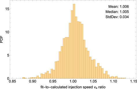
Figure 3. Ratio of the injection speed determined by fitting (Method 2) to that determined simply from the solar wind speed (Method 1). While the mean and median values are nearly identical, there is typically a few percent difference one way or the other.
Download figure:
Standard image High-resolution imageFigure 4 shows a scatter plot of reduced chi-squared for the two methods. The two give similar results for most of the 1-day histograms; however, fitting the injection speed produces a substantial quantitative improvement in the reduced chi-squared of numerous samples. Even more importantly, the largest improvements are for the worst fit points by Method 1. For these, the largest reduced chi-squared values of ∼20–150 are almost entirely improved to values of <20. Not surprisingly, these largest improvements correspond to the daily distributions that had the biggest discrepancies between the two injection speed values (reds and blues).

Figure 4. Scatter plot of reduced chi-squared including fitting the injection speed (Method 2) vs. simply using the calculated value (Method 1). The ratio between these two is color-coded. While most of the samples are similar (densely overplotted region on the left), the largest values are significantly improved by the fitting procedure.
Download figure:
Standard image High-resolution imageDetermination of the cooling index and the overall quality of the fit to the PUI distribution are both quite sensitive to knowledge of the injection speed, with a significantly tighter distribution of α values and fewer outliers when we use fitting to also determine the injection speed. We note that this fitting method should not be used to infer the actual solar wind bulk parameters, which are best determined from the fine E/q scans in SWAP (McComas et al. 2008; Elliott et al. 2016, 2018, 2019). However, as discussed above, there are physical reasons for the actual injection speed of the PUI distribution to have small variations from the difference between the bulk solar wind and inflowing ISN velocities. Thus, from here on in this study we examine properties of the PUI distributions and use the term "cooling index" and parameter α only to refer to the values derived from the fitting Method 2, which includes the additional injection speed fit parameter.
Another significant improvement in determining the pickup ion properties from SWAP in this study comes from how we integrate the distribution function to calculate the modeled count rates that are compared to the measured counts in our chi-squared minimization. McComas et al. (2017b) followed Equation (4) from Randol et al. (2013), which used a geometric factor appropriate for integration over energy. In this study, we follow Nicolaou et al. (2014) and Swaczyna et al. (2020) and use a geometric factor to integrate the modeled distribution over velocity space (see the Appendix). This method has an additional factor of one-half in the integration of the expected count rates based on the assumed distribution function. This factor of two correction in the integration leads to roughly two times higher pickup ion densities than found in the prior studies of Randol et al. (2013) and McComas et al. (2017b). This correction is further substantiated by that fact that using this same integration and forward-modeling process returns the same densities, on average, for the bulk solar wind as found in an independent analysis of the SWAP E/q fine scans by Elliott et al. (2016, 2018, 2019).
Finally, from the full SWAP data set of 2424 days of observations we cull data points that meet any of the following criteria: (1) fewer than 12 measurements of solar wind properties using the fine E/q sweeps from Elliott et al. (2019; this requirement eliminates 403 days), (2) variation of the solar wind speed from the fine sweep observations in a day greater than 1% (this requirement eliminates 253 days), or (3) a significant PUI tail above the H PUI cutoff (we define by a count rate in the lowest bin above 5 times the energy of the SW proton peak over one 1 count s–1; this requirement eliminates 162 days). Because some samples failed more than one test, this culling leaves 1758 daily histograms in our data set for further statistical study.
3. Pickup Ion Heating
Figure 5 shows the distribution of cooling index values for the 1758 daily histograms used in this study. Values of the cooling index vary from 1 all the way up to 4 with both mean and median values of ∼2.1. Fully 93.6% of all values are over 1.5—the value that indicates adiabatic expansion. Cooling index values are 15 times more common above 1.5 than below this value, indicating that additional heating of the PUIs during their outward expansion through the heliosphere is almost always occurring.

Figure 5. Probability distribution of cooling index (α) values. Adiabatic cooling, α = 3/2, is indicated by the dashed line. The vast majority (93.6%) indicate additional heating of the PUIs, with both mean and median values of ∼2.1 over the entire eight year interval.
Download figure:
Standard image High-resolution imageWe now turn to the physical meaning of the cooling index and source of this additional heating. We examine the correlation between α and other PUI and core solar wind parameters. Because the energy density of the PUIs is much larger than that in the core solar wind thermal energy or magnetic field, the energy for this additional heating must ultimately originate from the only source large enough to supply it—the flow energy density or dynamic pressure (1/2ρv2) of the outflowing solar wind. Because heating of the core solar wind is often associated with compressions and shocks in the solar wind, many of which are mostly produced by recurrent fast streams and CIRs, we first look there.
Table 1 lists 39 shocks and other compressions in the SWAP data between 22 and 46.6 au. To be included in the list, we required a significant jump in solar wind speed as defined by a measured solar wind speed increase of more than 14 km s−1 day−1 between any two observations. We chose this value empirically by looking at speed variations throughout the 8 yr of SWAP data. In addition to requiring a sufficiently large speed jump from one day to the next, we also manually scanned all of the possible intervals and culled out ones that did not have reasonably good data coverage and fitting of both solar wind and PUI parameters for the several days before and after the shock arrival itself, so this represents only a partial list.
Table 1. Interplanetary Shocks and Compressional Waves
| # | Year | DOY | r | Δv/Δt |
|---|---|---|---|---|
| (au) | (km s−1 day−1) | |||
| 1 | 2012 | 82 | 22.7 | 15.4 |
| 2 | 2012 | 89 | 22.7 | 21.6 |
| 3 | 2013 | 72 | 25.7 | 14.1 |
| 4 | 2014 | 282 | 30.6 | 15.7 |
| 5 | 2014 | 322 | 30.9 | 17.5 |
| 6 | 2015 | 67 | 31.8 | 22.1 |
| 7 | 2015 | 88 | 32.0 | 25.7 |
| 8 | 2015 | 113 | 32.2 | 14.7 |
| 9 | 2015 | 225 | 33.2 | 24.3 |
| 10 | 2015 | 262 | 33.5 | 29.8 |
| 11 | 2015 | 359 | 34.3 | 37.8 |
| 12 | 2016 | 13 | 34.4 | 18.2 |
| 13 | 2016 | 38 | 34.6 | 24.4 |
| 14 | 2016 | 77 | 35.0 | 32.5 |
| 15 | 2016 | 111 | 35.2 | 28.7 |
| 16 | 2016 | 140 | 35.5 | 30.6 |
| 17 | 2016 | 230 | 36.2 | 66.6 |
| 18 | 2016 | 253 | 36.4 | 21.9 |
| 19 | 2016 | 286 | 36.7 | 35.1 |
| 20 | 2016 | 307 | 36.8 | 26.1 |
| 21 | 2016 | 331 | 37.0 | 26.1 |
| 22 | 2016 | 356 | 37.3 | 16.0 |
| 23 | 2017 | 13 | 37.4 | 27.7 |
| 24 | 2017 | 44 | 37.7 | 15.3 |
| 25 | 2017 | 61 | 37.8 | 16.0 |
| 26 | 2017 | 88 | 38.1 | 14.2 |
| 27 | 2017 | 113 | 38.3 | 22.6 |
| 28 | 2017 | 201 | 39.0 | 19.1 |
| 29 | 2017 | 223 | 39.2 | 22.0 |
| 30 | 2017 | 281 | 39.6 | 15.4 |
| 31 | 2017 | 331 | 40.0 | 14.3 |
| 32 | 2017 | 351 | 40.2 | 24.6 |
| 33 | 2018 | 92 | 41.1 | 35.2 |
| 34 | 2018 | 120 | 41.3 | 14.3 |
| 35 | 2018 | 169 | 41.7 | 14.7 |
| 36 | 2019 | 42 | 43.6 | 15.5 |
| 37 | 2019 | 62 | 43.8 | 23.9 |
| 38 | 2019 | 116 | 44.2 | 19.5 |
| 39 | 2020 | 11 | 46.3 | 15.0 |
Download table as: ASCIITypeset image
Figure 6 shows the time series of various solar wind and PUI parameters over the 2 yr subset of the data from 2016 to 2017. Dashed lines indicate shocks or compressions from Table 1. Immediately after solar wind speed jumps (panel (a)), the solar wind density (panel (b)), solar wind temperature (panel (c)), PUI density (panel (d)), and PUI temperature (panel (e)) all generally increased, although there is significant variability in the response of these various parameters from one shock/compression to the next. In general, the PUI density and temperature appear to be more strongly correlated with the speed jumps than do the core solar wind parameters. Finally, the cooling index (panel (f)) is also generally enhanced after these speed jumps but appears to be slightly delayed compared to speed jumps and response of the other parameters.

Figure 6. Plots of solar wind and PUI parameters for 2016 and 2017 while NH traveled from 34.3 to 40.3 au. The panels show (a) solar wind speed, (b) solar wind density, (c) solar wind temperature, (d) PUI density, (e) PUI temperature, and (f) PUI cooling index. Significant jumps in the solar wind speed, indicative of shocks or waves (Table 1), are identified by the thin vertical lines.
Download figure:
Standard image High-resolution imageIn order to reduce the event-to-event variability and identify any systematic variations, we performed a superposed epoch analysis. Figure 7 shows this analysis using the epoch of the speed jumps for all 39 shocks and waves from 22.7 to 46.3 au, listed in Table 1. We include error bars that are calculated as standard error of the mean (i.e., the standard deviation from the set divided by the square root of the number of observations). Thus, for each point compared to the epoch, smaller error bars in this figure indicate less variability of the daily parameter values.

Figure 7. Superposed epoch analysis based on the solar wind speed jumps for the 39 shocks/waves identified in Table 1 (panel (a)). Solar wind density (panel (b)) and temperature (panel (c)) as well as PUI density (panel (d)) and temperature (panel (e)) all change discontinuously across the jumps and trend back to lower values over time. The PUI cooling index (panel (f)) responds differently, peaking about 1 week on average after the shocks/waves pass by.
Download figure:
Standard image High-resolution imageThe superposed epoch analysis bears out the correlations qualitatively seen in Figure 6. However, with the advantage of assembling multiple, variable structures with respect to their superposed epochs, we are able to quantitatively determine the average temporal variation of the various solar wind and PUI properties around such shocks and compressions. It is clear that the PUI density and both the core solar wind and PUI temperatures (panels (c)–(e)) jump up at the time of the solar wind speed jump (panel (a)) and then drop back down over the following 2–3 weeks. The core solar wind density (panel (b)) shows a more complicated time series (and larger error bars) but is elevated for the 2–3 weeks after the jumps compared to before then.
Unlike the immediate enhancements of solar wind and PUI densities and temperatures following the shocks/waves, we do not see the cooling index similarly increase either in the detailed comparisons (Figure 6) or in the superposed epoch analysis (Figure 7). Instead, the cooling index is only slightly enhanced across the shocks/waves but increases steadily to a peak value a week after the zero epoch. Thereafter, it decreases steadily over the following week roughly symmetrically with how it rose.
Table 2 provides the quantitative results from the superposed epoch analysis shown in Figure 7. In particular, for each parameter, we provide the value for the day before the zero epoch, the value for the day after, the percentage increase, the average value over the 10 days following the zero epoch, and the percentage increase in that value compared to the day before the zero epoch. Solar wind dynamic pressure and solar wind and PUI thermal pressures are calculated across the 39 shocks/compressions separately before averaging through the epoch analysis.
Table 2. Average Solar Wind and PUI Properties from Superposed Epoch Analysis
| Day Before | Day After | Increase | Average 1–10 Days After | 10-day Average Increase | |
|---|---|---|---|---|---|
| vSW [km s−1] | 388 ± 7 | 425 ± 8 | 9.3% | 418 ± 1 | 7.5% |
| nSW [10−3 cm−3] | 6.5 ± 0.7 | 7.4 ± 0.8 | 14.0% | 8.0 ± 0.2 | 22.0% |
| TSW [103 K] | 5.9 ± 0.8 | 13.7 ± 1.7 | 133% | 13.4 ± 0.5 | 128% |
| nPUI [10−3 cm−3] | 0.60 ± 0.04 | 0.88 ± 0.06 | 46.0% | 0.86 ± 0.01 | 42.9% |
| TPUI [106 K] | 3.96 ± 0.12 | 5.32 ± 0.24 | 34.2% | 4.97 ± 0.05 | 25.6% |
PSW‐Dyn = 1/2mp
 [fPa] [fPa] | 810 ± 80 | 1130 ± 120 | 38.5% | 1160 ± 30 | 42.2% |
| PSW = nSW kB TSW [fPa] | 0.48 ± 0.06 | 1.35 ± 0.19 | 183% | 1.30 ± 0.04 | 173% |
| PPUI = nPUI kB TPUI [fPa] | 32.4 ± 1.7 | 64.0 ± 4.8 | 97.7% | 58.0 ± 0.8 | 79.1% |
| αPUI a | 1.91 ± 0.07 | 2.01 ± 0.10 | 5.1% | 2.32 ± 0.02 | 21.4% |
Note.
a αPUI peaks with a value of 2.6 ± 0.1 (36% increase) 7 days after the zero epoch.Download table as: ASCIITypeset image
Subsequent studies will examine individual shocks and compressions to explore the variety of detailed structure of these important observations. Here we use the superposed epoch results to briefly examine the average, or typical, structure. Compression (density downstream/upstream) ratios for the superposed epoch analysis range from 1.14 and 1.22 for the solar wind density for the 1 day after and 10-day average after the shock/wave passage, respectively, to 1.46 and 1.43 for the PUI densities over the same intervals. We compare these values to the single relatively strong shock (PUI compression ratio of 3.0) already studied in detail using SWAP observations at ∼34 au (Zirnstein et al. 2018b). Not surprisingly, the superposed epoch composite has a much smaller compression ratio, as it averages together large and small shocks with likely some nonshock compressions.
Using the continuity equation and PUI densities, we calculate the average shock/wave speed in the Sun frame V = (nPUId vSWd–nPUIu vSWu)/(nPUId–nPUIu), with upstream (u) to downstream (d) values. This calculation gives a speed of the superposed epoch disturbance of 504 km s−1. Now we can convert the flows into the shock frame and examine the energy balance as Zirnstein et al. (2018b) did, but for the composite, averaged shock/wave structure. Assuming perpendicular shocks, we find that the energy density flux of solar wind H+ is 8.7 and 3.4 pPa km s−1 upstream and downstream, respectively, and the energy flux of PUI H+ is 10.3 and 13.2 pPa km s−1. This shows that the PUI energy flux increases significantly across the shocks, whereas the core solar wind ion energy flux does not. By estimating the upstream magnetic field magnitude as 0.15 nT based on Voyager observations (Bagenal et al. 2015) and taking the average compression ratio from PUI density across the shock from Table 2, the total energy flux upstream and downstream of the shock is 21.1 and 19.6 pPa km s−1, respectively. The difference in energy flux across the shock is small (∼7%) and is likely explained by the small remaining contribution from electrons, alphas, and PUI He+ that we have not accounted for. Thus, similar to the analysis of Zirnstein et al. (2018b), the total energy flux is approximately conserved across the epoch-averaged shocks observed by SWAP, with PUI H+ containing a significant amount of the energy flux (almost 70% of solar wind H+ + PUI H+ + magnetic energy flux).
4. Radial Variations of PUI Properties
Over the 8 yr from 2012 January 28 through 2020 January 28, New Horizons transited from ∼22 out to almost 47 au, nearly continuously measuring the PUIs through this distant region of the heliosphere for the first time. As described in Section 2, for our quantitative analysis we iteratively forward-modeled PUI distributions and minimized chi-squared differences between these and the daily histogram observations. We culled out samples that failed any of several completeness or quality tests. The remaining 1758 daily samples that meet all criteria required by our analysis process represent 60.2% coverage over this time range. This large sampling is roughly evenly distributed, so it provides an excellent data set for examining the characteristic variations of PUIs across this large range of heliocentric distances.
Figure 8 shows the individual daily measurements of the PUI H+ density, temperature, thermal pressure, and cooling index (gray points) as a function of heliocentric distance. Because of the large variability in the solar wind, we also average these values over solar rotations, which helps to reduce the effects of variable sampling of faster and slower parcels of source solar wind plasma emitted from different solar longitudes. The solar rotation rate varies from ∼24.5 days at the equator to nearly 38 days at the poles, with an average of ∼28 days; while the exact value does not make much difference in the averages, here we use a somewhat standard 27.3 days. The black dots show these average values, and the black vertical bars indicate the ±1σ variability over each solar rotation.
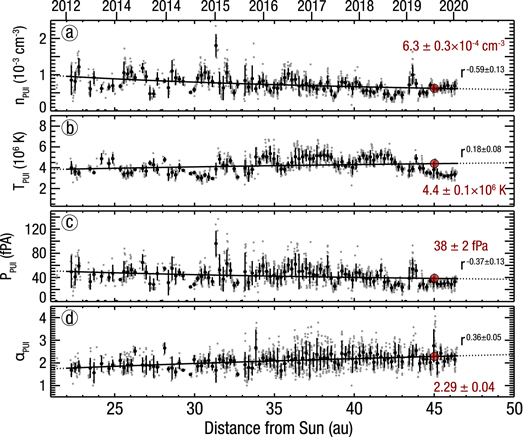
Figure 8. Individual values of daily-averaged PUI observations (gray dots) that pass all of the described quality checks. Vertical bars show ±1σ variability over individual 27.3-day solar rotation averages (black dots) for all rotations where there are at least 10 samples in that interval. We provide power-law fits for the solar rotation averaged values over the nearly continuous observations from 22 to 47 au (solid lines) and "fiducial" values for each parameter at 45 au (red dots and values).
Download figure:
Standard image High-resolution imageThe black solid lines in Figure 8 show power-law fits of the radial profiles using the 27.3-day solar rotation averages of the SWAP observations. Solar wind variations evolve as they move outward but always significantly exceed instrumental uncertainties. Consequently, time variations of these parameters cannot be used as a measure of data uncertainty. The real experimental uncertainties are small and comparable for each solar rotation average. Because deviations of the averages from the power-law fits result from measuring differing parcels of solar wind rather than observational uncertainties, we use unweighted fits that treat the values from each solar rotation equally.
The PUI density and thermal pressure both drop off with heliocentric distance, with radial gradients of r−0.59 and r−0.37, respectively. In contrast, the PUI temperature increases as r+0.18, while the new addition to our PUI fitting procedure, the cooling parameter α, increases with a radial gradient of r+0.36—an exponent twice that of the PUI temperature itself. In addition to the radial trends, we provide best-fit values for the four PUI parameters in Figure 8 at 45 au (red dots), roughly halfway out to the termination shock.
The temperature for the PUI distribution function given in Equation (2) depends on the cooling index, solar wind speed, injection speed, and distance from the Sun. We examine the relationship between the PUI temperature and cooling index in Figure 9. Panel (a) shows the PUI temperature as a function of solar wind speed, color-coded by the heliocentric distance of each observation. Overall, this plot shows how closely the temperature and speed are correlated, with higher speeds associated with higher temperatures. This correlation is related to the relation of the injection speed, which scales velocities of PUIs, to the solar wind speed. Additionally, higher speeds go with stream interactions and compressions that heat both the core solar wind plasma and PUIs as shown in detail above.

Figure 9. Pickup ion temperatures as a function of solar wind speed color-coded by (a) heliocentric distance and (b) cooling index, α.
Download figure:
Standard image High-resolution imageFigure 9(b) again shows PUI temperature as a function of solar wind speed, but this time color-coded by the cooling index, α. This plot shows a clear relationship where, in addition to the speed–temperature correlation, at each speed, the higher temperatures are associated with the higher cooling indices and lower temperatures with lower cooling indices. The temperature and cooling index are related to each other through Equation (2), which explains some of the correlation. However, the measured solar wind speed is different from the injection speed fit value as described above, so these two parameters are formally independent. In any case, it makes sense for higher cooling indices to be associated with higher PUI temperatures, as they indicate greater heating of the PUIs.
Next, we turn to the ratios of the PUI to core solar wind parameters as a function of distance. In our earlier study we separately fit the solar wind and PUI radial gradients and then took the ratios of these. For this study, we introduce a significant improvement as shown in Figure 10. Here, we take the ratios of the parameters on a daily point-by-point basis (gray). This is better because the charge exchange rate is linearly related to the local plasma density, so the ratio takes out first-order variations in the solar wind densities and pressures. We then make the 27.3-day solar rotation averages (black), as in Figure 8, and again fit a power law to these averages. For these fits, we do use the statistical variability of the points since some of the variations in the solar wind parameters have already been removed by using the ratios and much of what is left is due to actual statistical fluctuations. Again, we provide 45 au fiducial values (red) for each of these ratios.
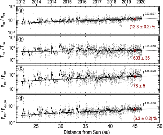
Figure 10. Ratios of various parameters taken for individual daily measurements and then processed and plotted as in Figure 8. The panels show ratios of (a) solar wind (SW) to total (Tot, combined PUI and solar wind) density, (b) PUI to solar wind temperatures, (c) PUI to solar wind thermal pressures, and (d) the PUI thermal pressure to the solar wind dynamic pressure.
Download figure:
Standard image High-resolution imageTable 3 summarizes the parameters (Figure 8) and ratios (Figure 10) at 45 au, their power-law radial dependences, and extrapolations to the nominal upstream termination shock, twice as far out, at ∼90 au; we note that Voyager 1 crossed at ∼94 au (Stone et al. 2005) and Voyager 2 at ∼84 au (Stone et al. 2008). Errors are relatively small for the 45 au values because this distance is within the range of the new SWAP observations. In contrast, errors on the extrapolated values are significantly larger. This is because there is a nonnegligible correlation between the radial dependence of the fit parameters and the fraction of PUIs, which we include in our calculations.
Table 3. PUI Properties at 45 au, Radial Dependences, and Extrapolated Values at 90 au
| Value at 45 au | Extrapolated to 90 au | Radial Exponent | |
|---|---|---|---|
| nPUI | (6.3 ± 0.3) × 10−4 cm−3 | (4.1 ± 0.6) × 10−4 cm−3 | −0.59 ± 0.13 |
| TPUI | (4.4 ± 0.1) × 106 K | (5.0 ± 0.4) × 106 K | 0.18 ± 0.08 |
| PPUI | 38 ± 2 fPa | 30 ± 4 fPa | −0.37 ± 0.13 |
| α | 2.29 ± 0.04 | 2.9 ± 0.2 | 0.36 ± 0.05 |
| nPUI/nTotal | (12.3 ± 0.2)% | (24 ± 2)% | 0.97 ± 0.07 |
| TPUI/TSW | 603 ± 35 | 716 ± 124 | 0.25 ± 0.18 |
| PPUI/PSW | 78 ± 5 | 173 ± 32 | 1.15 ± 0.20 |
| PPUI/PSW–Dyn | (6.3 ± 0.2)% | (14 ± 1)% | 1.18 ± 0.08 |
Download table as: ASCIITypeset image
As described above, we averaged data points (and ratios of data values) over full solar rotations in order to minimize variability caused by differing solar wind sources at different solar longitudes. In order to make sure that the values and extrapolations were not strongly driven by this averaging interval, we also tested our analysis using data averaged over multiple integral numbers of solar rotations. While averaging over increasingly longer intervals becomes less defensible for characterizing the parameters at any given distance, we found that values were generally within the derived errors bars even when summing over multiple rotations.
Figures 8 and 10 and Table 3 provide a quantitative analysis of the first direct observations of PUIs beyond 38 au. Further, with the additional observations out to nearly 47 au, we now have sufficient data to well characterize the PUI properties more than halfway out to the termination shock. McComas et al. (2017b) found the PUI temperature increasing with heliocentric distance as ∼r+0.7 and a PUI thermal pressure that was increasing slightly with distance, although consistent with no radial change to within errors. By including the cooling index as a fitting parameter in this study, we better fit the PUI distribution function and no longer overestimate the PUI temperature at larger distances from the Sun. With this and the additional data from ∼38–47 au included, we now find a PUI temperature that is only slightly increasing (∼r0.18) and PUI pressure dropping off (∼r−0.37) with distance. The possibility of PUI pressure increasing with distance raised in our prior study was unexpected, and the updated result in this study is more in line with theoretical expectations.
The extrapolated PUI density at the termination shock in our earlier study (McComas et al. 2017b) was also significantly lower than anticipated. In the current study, as described above, we made a factor of two correction to the geometric factor used in our integration compared to our prior study and its predecessor (Randol et al. 2013). We now find that the PUI density is already 12% of the total combined density by 45 au and the power-law exponent of this percentage has a value of 1 to within errors. A linear increase in the fraction is not surprising, as, to first order, the PUI density should increase proportionally to distance (e.g., Lee et al. 2009). Thus, nPUI/nTotal of 24% at the termination shock should be a good estimate of the real value.
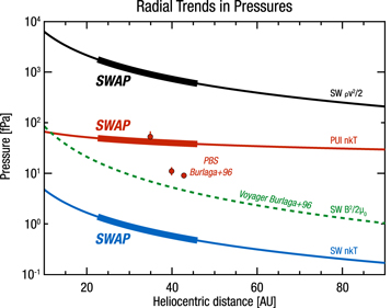
The ratios of PUI to solar wind temperatures and thermal pressures (TPUI/TSW and PPUI/PSW) are both quite large with 45 au values of 600 and 78, respectively. Figure 11 shows the best-fit values of the SWAP observations over ∼22–47 au (thick lines) and extrapolated values (thin lines). New Horizons does not have a magnetometer, so we have no direct measurements of the local magnetic pressure. Much earlier magnetic field observations from Voyager (e.g., Burlaga et al. 1996 dashed line) allowed McComas et al. (2017b) to show that the PUI pressure overtakes the magnetic pressure well inside 20 au. By the time the solar wind reaches 45 au, the PUI pressure should be a decade or more larger than magnetic pressure, making the field pressure largely inconsequential farther out in the heliosphere.
Figure 11. SWAP solar wind and PUI observations from ∼22–47 au (thick lines) and extrapolated radial trends (thin lines). The red line shows the PUI thermal pressure, directly plotting the power-law fit with the parameters given in Table 3. The black line shows the solar wind dynamic pressure, determined by PPUI /(PPUI/PSW‐Dyn), where both the numerator and denominator come from power-law fits in Table 3. The blue line shows the SW thermal pressure, calculated in a similar way via PPUI /(PPUI/PSW). The magnetic pressure radial variation was measured by Voyager (green dashed line; Burlaga et al. 1996). Those authors also inferred values of PUI pressure from measurements of three pressure balance structures (PBSs; red dots).
Download figure:
Standard image High-resolution image
As shown above and summarized in Figure 11, the dominance of the PUI thermal pressure continues to increase with heliocentric distance and even becomes a significant fraction of the solar wind dynamic pressure, which is by far the largest pressure in the inner heliosphere. We find that the PUI pressure is already over 6% of the solar wind dynamic pressure by 45 au, and with the continuing addition of H+ PUIs, we show that this value should rise to ∼14% by the termination shock. Such a large value means that PUIs play a major and fundamental role in the physics of the termination shock.
5. Discussion and Conclusions
In this study we examine PUI observations from 38 to nearly 47 au from the SWAP instrument for the first time and reexamine observations from ∼22 to 38 au to provide significantly enhanced analysis of the H+ PUI properties and their radial variations. The observations span 8 yr from early 2012 to 2020 as New Horizons traveled near the VLISM upwind direction, toward the nose of the heliosphere (see Figure 1). With these new observations, we now have nearly continuous coverage over more than a factor of two in heliocentric distance.
We also provide "fiducial" values at 45 au, halfway to the nominal termination shock, and radial power-law fits and extrapolated values (Table 3). While we extrapolate out at 90 au to give characteristic values for the various parameters at the termination shock, we recommend that theories and models that characterize the radial variations of these parameters should generally seek to match the SWAP PUI observations at our 45 au fiducial values, as this will allow different functional forms for the radial evolution of the solar wind and PUIs beyond our current observations, consistent with such theories and models.
By including a new cooling index exponent, α, in the parameterization of the PUI distribution (Chen et al. 2014; Swaczyna et al. 2020), we are able to fit these distributions well over all heliocentric distances studied. In contrast, in our prior study (McComas et al. 2017b), we had to use unphysically large and small "fitting parameters" for the local ionization, βHF, and ionization cavity, λHF, in order to fit the PUI distributions. Here, with the inclusion of the physically motivated cooling index, we were able to use normal values for these two parameters and achieve very good fits for most of the measured distributions.
Using the extended set of the SWAP observations to nearly 47 au, we also repeated the calculations from Swaczyna et al. (2020) and find the interstellar hydrogen density at the heliopause of 0.127 ± 0.015 cm−3. In the previous study, the injection speed was not a fit parameter as discussed in Section 2; nevertheless, we verify that this development increases the obtained interstellar hydrogen density by only 2%, i.e., much less than the estimated uncertainty. Both the value and its uncertainty are exactly the same as found in the previous study, but we note that the statistical component of the uncertainty drops from 0.0011 cm−3 in Swaczyna et al. (2020) to 0.0007 cm−3 in this analysis. Since the total uncertainty is dominated by systematic uncertainties, the extended data in our current study do not significantly improve the total uncertainty. However, further continuous observations may give insights to possible discrepancies from the cold model of the ISN hydrogen distribution in the heliosphere, which is assumed in this approach.
The H PUI density extrapolated in this study to 90 au of (4.1 ± 0.6) × 10−4 cm−3 can be compared to the H PUI density obtained by Sokoł et al. (2019). Those authors adopted the density of ISN H at the termination shock of 0.0852 cm−3 and obtained an H PUI density of 2.26 × 10⁻⁴ cm−3. Since the expected H PUI density is proportional to the ISN H density, their density of H PUIs can be proportionally scaled to 2.26 × 10−4 × (0.127/0.0852) = 3.37 × 10⁻⁴ cm−3, which is closer to the extrapolated value found in this study.
The cooling index is greater than 1.5—the value that indicates adiabatic cooling—for the vast majority (93.6%) of the distributions. The cooling index increases with radial distance with a power-law exponent of 0.36, a 45 au fiducial value of 2.3, and an extrapolated value of 2.9 at the upstream termination shock. These results show additional heating of the PUI population progressively more with increasing distance from the Sun. This indicates that additional energy is routinely being extracted from the solar wind flow and injected into the PUI population. The preferential heating of the PUIs at least partially occurs from particle interactions at compressions and shocks, as shown in Figures 6 and 7 and studied in detail for a particular shock by Zirnstein et al. (2018b). SWAP observations clearly show the preferential heating of PUIs at interplanetary shocks out to ∼46 au from the Sun, where PUIs comprise a major fraction of the total energy flux of the downstream plasma in the shock frame. This is a direct indication that PUIs must also strongly mediate the termination shock, since the ratio of the PUI internal pressure to solar wind dynamic pressure is even larger upstream of the termination shock.
As pointed out by Zank et al. (2018) in a recent modeling analysis of the SWAP PUI observations out to 38 au, it is also possible that PUIs experience stochastic acceleration within the ambient and self-generated magnetic field turbulence (e.g., Bogdan et al. 1991; Le Roux & Ptuskin 1998; Isenberg 2005; Chalov et al. 2006; Fahr & Fichtner 2011; Gamayunov et al. 2012).
We showed preferential PUI heating in the shocks and compressions observed by SWAP. These are driven by faster solar wind overtaking slower solar wind as they travel through the outer heliosphere. This process produces compressions, some of which steepen into shocks. Many of these are associated with CIRs, which can eventually pile up into even larger MIRs. The speed differences continue to wear down, becoming smaller with heliospheric distance, but the plasma retains regions of higher temperatures and densities that persist as the plasma moves through the outer heliosphere.
Interestingly, our superposed epoch analysis showed that unlike the PUI and solar wind densities, temperatures, and thermal pressures, the cooling index does not peak until about a week after the passage of the speed jumps, increasing for the first week after and roughly symmetrically decreasing for the week after that. This behavior may derive from the larger scale and more integrative aspects of the PUI distribution, which is generated by progressive addition of fresh PUIs on the outermost pickup shell of the distribution in velocity space. For example, perhaps the delay in the cooling index peak indicates that it takes days to a week after the passage of a shock or compression for the PUI outer shell to build up from enhanced charge exchange in the higher-density downstream region. This would suggest that while some PUI heating occurs at the shock itself, additional heating from the enhanced PUI densities and their effect on low-frequency turbulence (Zank et al. 2018) could lag by about a week.
The set of 39 compressional waves and shocks identified for the superposed epoch analysis in this study are just a subset of these sorts of structures in our observations. For this study, we took a very conservative approach to fitting the PUI distributions and rejected daily samples that did not pass all of our described quality checks. We also manually rejected cases that were missing too many samples around the shock/wave speed jumps.
McComas et al. (2017b) showed that a number of traveling interplanetary shocks produce suprathermal PUI "tails" that extend significantly above the PUI cutoff energy. PUI tails associated with some shocks tend to produce bad fits to our model distribution. For example, the relatively large shock (compression ratio of 3) from 2015 October 5 (DOY 278) at ∼34 au studied by Zirnstein et al. (2018b) is not on our list, as it has a significant tail to higher energies. These authors showed that PUIs were preferentially heated compared to the core solar wind and that the PUIs, including their tail, contained roughly six times the energy flux of the core solar wind for this event.
While beyond the scope of this overview study, future analyses, which include the detailed shapes of the PUI distributions instead of relying on parameterized fits, should be able to examine such distributions and additional shocks/waves. These data are invaluable for future, more detailed studies of the effects of PUI pressure-dominated waves, shocks, and other structures.
Our SWAP observations provide critical information for understanding the heliosphere's termination shock in at least two ways. First, the shocks in our SWAP observations are the only examples of PUI-mediated shocks with direct observations of the PUIs, so they provide a critical and unique set of observations for understanding such shocks. Second, they are the only measurements of PUIs ever taken beyond ∼8 au and therefore allow us to accurately predict the average quantities immediately upstream of the termination shock.
By 45 au, the PUI thermal pressure is already over 6% that of core solar wind dynamic pressure, and at the upstream termination shock it is likely ∼14% of the dynamic pressure. This ratio provides a measure of how strongly the PUIs weaken and mediate the shock structure. The large fraction found here has profound implications for the termination shock, which was seen to be strongly mediated by Voyager 2 (Zank et al. 1996, 2010; Richardson et al. 2008; Mostafavi et al. 2017); we note, however, that Voyager 2 is unable to measure interstellar PUIs, so their distributions across the termination shock were not measured as they are for the interplanetary shocks observed by SWAP. Beyond the termination shock, PUI-mediated shocks are common across other astrophysical settings. Because the SWAP observations provide the only direct observations of PUI acceleration and heating associated with such structures, they are even more critical for the general physical understanding of PUI-mediated shocks across the cosmos.
Turning now to the solar wind conditions just upstream of the termination shock, we find the ratio of the H+ PUI density to the combined PUI and core solar wind density at the upstream termination shock to be ∼24%. This value is roughly twice that found in our previous study (McComas et al. 2017b), largely owing to the factor of two correction in the integration of the PUI distribution (Appendix). This larger value is far more consistent with theoretical expectations from various models. For example, PUI density ratios extracted from global heliosphere models by Malama et al. (2006), Zirnstein et al. (2017), and Heerikhuisen et al. (2019) predict PUI density ratios between ∼20% and 25% near the upstream TS (which is closer to ∼30% if the models underestimate the higher ISN H density determined from SWAP observations; Swaczyna et al. 2020).
A significant improvement to the SWAP observations will occur in 2021 May, when updated flight software will begin to produce 1 hr distribution functions instead of the current 1-day samples. This higher cadence will be a huge improvement for studying compressions, shocks, and other structures in the solar wind and will provide considerable additional opportunity for new exploration science of the detailed PUI distributions in the outer heliosphere as New Horizons continues to transit outward at nearly 3 au per year. Based on initial power projections, New Horizons has enough power to be operational until it reaches somewhere between 90 and 110 au (Stern et al. 2018).
In early 2025, NASA's Interstellar Mapping and Acceleration Probe (IMAP) mission (McComas et al. 2018) will launch to explore particle acceleration in the solar wind and its connection to the outer heliosphere and the heliosphere's interaction with the VLISM. SWAP observations from New Horizons (over 60 au from the Sun when IMAP launches) are ideally located in the outer heliosphere and are extremely useful for tying together IMAP's 1 au in situ data with its remote observations of the PUIs in the heliosheath, after they have been processed through the termination shock.
This paper serves as the citable reference for use of the SWAP PUI observations out to ∼47 au by the broader scientific community. These data can be accessed through the Space Physics at Princeton website (https://spacephysics.princeton.edu/missions-instruments/swap/pui-data-2021), and will be made available through the NASA SPDF repository. Researchers are also strongly encouraged to reach out and work directly with the SWAP team on other analyses and comparisons to more detailed theories and models going forward.
We gratefully thank all of the SWAP instrument and New Horizons mission team members and are especially grateful to Cathy Olkin for her contributions in making the New Horizons mission possible. We are disclosing that S.A.S., J.S., K.S., and H.W. were added as coauthors at the direction of the New Horizons mission PI and are not to be held responsible for the scientific observations, analysis, or results of this study. This work was carried out as a part of the SWAP instrument effort on the New Horizons project, with support from NASA's New Frontiers Program.
Appendix: Calculating Forward-modeled Count Rates
Differential fluxes,  , of particles can be estimated from the observed count rates, c, using the following formula (e.g., Nicolaou et al. 2014):

assuming that the differential flux is constant within the energy bin, ΔE, and the FOV, ΔΩ. The effective area, Aeff, accounts for the instrument aperture area and includes detection efficiencies. An energy geometric factor, GE (e.g., Funsten et al. 2009), is defined as

This approximation is useful since the energy resolution or relative width of ΔE/E is approximately constant for ESA-based instruments. Thus, the energy geometric factor is mostly energy independent. Nevertheless, the increase of this geometry factor due to postacceleration in SWAP (Randol et al. 2013) is accounted for in this study.
Following the transformation between flux and the distribution function f (e.g., Nicolaou et al. 2014, Equation (3)),

we provide the final count rate formula (e.g., Nicolaou et al. 2014, Equation (5)) as

We note that this equation does not agree with Equation (4) in Randol et al. (2013), which omits the factor of 1/2 (after integration over φ). The SWAP PUI analysis in McComas et al. (2017b) followed the Randol et al. (2013) equation, and therefore it also missed the factor of 1/2.
In the current study we resolve this discrepancy and adopt the correct transformation of the modeled distribution function to expected count rates at SWAP to include this factor of 1/2 in the integration over speed, as in Swaczyna et al. (2019, 2020).
We also note that the confusion may have arisen because two different geometric factors have been used in the literature. Johnstone et al. (1987) used velocity geometric factor, Gv , which is defined as

Transforming the variables from speed to energy, one can show that
Comparing the velocity and energy geometric factor, one can easily notice that they are related as

This again shows the factor of 1/2 needed to convert between energy and velocity geometric factors.