


Abstract
We report the discovery of 41 new high-z quasars and luminous galaxies that were spectroscopically identified at 5.7 ≤ z ≤ 6.9. This is the fourth in a series of papers from the Subaru High-z Exploration of Low-Luminosity Quasars (SHELLQs) project, based on the deep multi-band imaging data collected by the Hyper Suprime-Cam (HSC) Subaru Strategic Program survey. We selected the photometric candidates using a Bayesian probabilistic algorithm and then carried out follow-up spectroscopy with the Gran Telescopio Canarias and the Subaru Telescope. Combined with the sample presented in the previous papers, we have now spectroscopically identified 137 extremely red HSC sources over about 650 deg2, which includes 64 high-z quasars, 24 high-z luminous galaxies, 6 [O iii] emitters at z ∼ 0.8, and 43 Galactic cool dwarfs (low-mass stars and brown dwarfs). The new quasars span in luminosity range from M1450 ∼ −26 to −22 mag, and continue to populate luminosities a few magnitudes lower than have been probed by previous wide-field surveys. In a companion paper, we derive the quasar luminosity function at z ∼ 6 over an unprecedentedly wide range of M1450 ∼ −28 to −21 mag, exploiting the SHELLQs and other survey outcomes.
Export citation and abstract BibTeX RIS
1. Introduction
High-z quasars24 are an important probe of the early universe in many ways. Their rest-ultraviolet (UV) spectra blueward of Lyα are very sensitive to the H i absorption, and thus indicate the progress of cosmic reionization through the neutral fraction of the intergalactic medium (IGM; Gunn & Peterson 1965; Fan et al. 2006). The very existence of such objects puts strong restrictions on, and sometimes even challenges, models of the formation and early evolution of supermassive black holes (SMBH; e.g., Volonteri 2012; Ferrara et al. 2014; Madau et al. 2014). High-z quasars are also used to probe the assembly of the host galaxies, which are thought to form in the highest density peaks of the dark matter distribution in the early phase of cosmic history (e.g., Goto et al. 2009; Decarli et al. 2017).
Previous surveys have identified more than 100 high-z quasars so far (e.g., Bañados et al. 2016, and references therein), with the most distant objects known at z = 7.54 (Bañados et al. 2018) and z = 7.085 (Mortlock et al. 2011). However, most of the known quasars have redshifts z < 6.5 and UV absolute magnitudes M1450 < −24 mag, while higher redshifts and fainter magnitudes remain largely unexplored. There must be numerous objects of faint quasars and active galactic nuclei (AGNs) behind the known luminous quasars; they may represent the more typical mode of SMBH growth in the early universe, and may have made a significant contribution to reionization.
For the past few years, we have been carrying out a high-z quasar survey with the Subaru 8.2 m telescope. We have already reported discoveries of 33 high-z quasars, along with 14 high-z luminous galaxies, 2 [O iii] emitters at z ∼ 0.8, and 15 Galactic brown dwarfs, in Matsuoka et al. (2016, 2018, Paper I and II, hereafter). Multi-wavelength follow-up observations of the discovered objects are ongoing, whose initial results from the Atacama Large Millimeter/submillimeter Array (ALMA) data are presented in Izumi et al. (2018, Paper III). This "Subaru High-z Exploration of Low-Luminosity Quasars (SHELLQs)" project is based on the exquisite multi-band photometry data collected by the Hyper Suprime-Cam (HSC) Subaru Strategic Program (SSP) survey (Aihara et al. 2018a). HSC is a wide-field camera on the Subaru Telescope, and has a nearly circular field of view of 1 5 diameter, covered by 116 2K × 4K Hamamatsu fully depleted CCDs, with the pixel scale of 0
 17 (Miyazaki et al. 2018). The camera dewar design and on-site quality assurance design are described in Komiyama et al. (2018) and Furusawa et al. (2018), respectively. The HSC-SSP survey has three layers with different combinations of area and depth. The Wide layer is observing 1400 deg2 mostly along the celestial equator, with 5σ point-source depths of (gAB, rAB, iAB, zAB, yAB) = (26.5, 26.1, 25.9, 25.1, 24.4) mag measured in 20 aperture. The Deep and the UltraDeep layers are observing smaller areas (27 and 3.5 deg2) down to deeper limiting magnitudes (rAB = 27.1 and 27.7 mag, respectively). The observed data are processed with the dedicated pipeline hscPipe (Bosch et al. 2018), which was developed from the Large Synoptic Survey Telescope software pipeline (Jurić et al. 2015). The HSC pipeline is evolving through the period of the survey, which sometimes gives rise to somewhat inconsistent photometry (and the quasar probability of a given source; see below) between different data releases. A full description of the HSC-SSP survey can be found in Aihara et al. (2018a).
This paper is the fourth in a series of SHELLQs publications, and reports spectroscopic identification of an additional 73 objects in the latest HSC-SSP data. We describe the photometric candidate selection briefly in Section 2, while a more complete description may be found in Papers I and II. The spectroscopic follow-up observations are described in Section 3. The quasars and other classes of objects we discovered are presented in Section 4. A summary appears in Section 5. A companion paper (Y. Matsuoka et al. 2018, in preparation) describes the quasar luminosity function at z ∼ 6 derived from the SHELLQs sample obtained so far. This paper adopts the cosmological parameters H0 = 70 km s−1 Mpc−1, ΩM = 0.3, and ΩΛ = 0.7. All magnitudes in the optical and NIR bands are presented in the AB system (Oke & Gunn 1983), and are corrected for Galactic extinction (Schlegel et al. 1998). We use two types of magnitudes; the point-spread function (PSF) magnitude (mAB) is measured by fitting PSF models to the source profile, while the CModel magnitude (mCModel,AB) is measured by fitting PSF-convolved, two-component galaxy models (Abazajian et al. 2004). We use the PSF magnitude error (σm) measured by the HSC data processing pipeline (Bosch et al. 2018); it does not contain photometric calibration uncertainty, which is estimated to be at least 1% (Aihara et al. 2018b). In what follows, we refer to z-band magnitudes with the AB subscript ("zAB"), while redshift z appears without a subscript.
2. Photometric Candidate Selection
Our photometric candidate selection starts from the HSC-SSP source catalog. We used the survey data in the three layers, observed before 2017 May, i.e., a newer data set than that contained in the latest public data release (Aihara et al. 2018b). We required that our quasar survey field has been observed in the i, z, and y bands (not necessarily to the full depths; see below), but impose no requirement on the g- or r-band coverage. All sources meeting the following criteria, without critical quality flags (see Paper I), are selected:
or

Here, we use the difference between the PSF and CModel magnitudes (mAB–mCModel,AB) to reject extended sources. With the present threshold value (0.15), our completeness of point-source selection is >80% at zAB < 24.0 mag (Paper II). The completeness decreases toward fainter magnitude, which should be accounted for in statistical measurements (e.g., luminosity function) of the discovered quasars. We further remove sources with more than 3σ detection in the g- or r-band, if these bands are available, as such sources are most likely low-z interlopers.
Next, we process the HSC images of the above sources through an automatic image-checking procedure, in all the available bands. As detailed in Papers I and II, this procedure uses Source Extractor (Bertin & Arnouts 1996), and removes those sources whose photometry is not consistent (within 5σ significance) between the stacked and all the pre-stacked, individual images. We also eliminate sources with too-compact, diffuse, or elliptical profiles to be celestial point sources on the stacked images. The sources removed at this stage are mostly cosmic rays, moving or transient sources, or image artifacts.
The candidates selected above are matched, within 10 separation, to the public near-IR catalogs from the United Kingdom Infrared Telescope Infrared Deep Sky Survey (Lawrence et al. 2007), the Visible and Infrared Survey Telescope for Astronomy (VISTA) Kilo-degree Infrared Galaxy survey, the VISTA Deep Extragalactic Observations Survey (Jarvis et al. 2013), and the UltraVISTA survey (McCracken et al. 2012). The choice of the 10 matching radius is rather arbitrary, but is at least sufficiently larger than the astrometric uncertainties of the above surveys. Then, using the i, z, and y-band magnitudes along with all the available J, H, and/or K magnitudes, we calculate Bayesian quasar probability ( ) for each candidate, based on spectral energy distribution (SED) models and estimated surface densities of high-z quasars and contaminating brown dwarfs as a function of magnitude. Our algorithm does not contain galaxy models at present. We created the quasar SED models by stacking the SDSS spectra of 340 bright quasars at z ≃ 3, where the quasar color selection is fairly complete (Richards et al. 2002; Willott et al. 2005), and correcting for the effect of IGM absorption (Songaila 2004). The quasar surface density was modeled with the luminosity function of Willott et al. (2010). The color models of brown dwarfs were computed with a set of observed spectra compiled in the SpeX prism library,25
and the CGS4 library,26
while the surface densities were calculated following Caballero et al. (2008). A more detailed description of our Bayesian algorithm may be found in Paper I. We reject sources with PQB < 0.1, and keep those with higher quasar probabilities in the sample of candidates.
) for each candidate, based on spectral energy distribution (SED) models and estimated surface densities of high-z quasars and contaminating brown dwarfs as a function of magnitude. Our algorithm does not contain galaxy models at present. We created the quasar SED models by stacking the SDSS spectra of 340 bright quasars at z ≃ 3, where the quasar color selection is fairly complete (Richards et al. 2002; Willott et al. 2005), and correcting for the effect of IGM absorption (Songaila 2004). The quasar surface density was modeled with the luminosity function of Willott et al. (2010). The color models of brown dwarfs were computed with a set of observed spectra compiled in the SpeX prism library,25
and the CGS4 library,26
while the surface densities were calculated following Caballero et al. (2008). A more detailed description of our Bayesian algorithm may be found in Paper I. We reject sources with PQB < 0.1, and keep those with higher quasar probabilities in the sample of candidates.
Finally, we inspect the images of all the candidates by eye and remove additional problematic sources. About 80% of the remaining candidates were rejected at this last stage, and were mostly cosmic rays but also included transient/moving objects and sources close to bright stars. The latest HSC-SSP (internal) data release covers 650 deg2, when we limit to the field where at least a single exposure in the i and two exposures each in the z and y bands were obtained. From the final sample of candidates, we put the highest priority for spectroscopic identification on a subsample with relatively bright magnitudes (zAB < 24.0 mag or yAB < 23.5 mag), red colors (iAB − zAB > 2.0 or zAB − yAB > 0.8), and detection in more than a single band (for i-dropouts) or a single exposure (for z-dropouts). The number of photometric candidates is changing throughout the survey, due to the continuous arrival of new HSC-SSP survey data, a change in the photometry and quasar probability ( ) with updates of the data processing pipeline, and the progress of our follow-up spectroscopy.
The present HSC survey footprint includes 15 high-z quasars discovered by other surveys, as summarized in Table 1. We recovered 10 of these quasars with  , while three quasars were not selected due to their relatively low redshifts (z < 5.9) and bluer HSC colors (iAB − zAB < 1.5) than the HSC color selection threshold described above. The remaining two quasars are missing due to nearby bright sources; VIK J0839+0015 is assigned with an HSC pixelflags_bright_objectcenter flag (indicating that the pipeline measurements of this source may be affected by a nearby bright source) and therefore does not meet the HSC source selection criteria described above, while SDSS J1602+4228 is rejected in our automatic image-checking procedure, since its i-band photometry is not consistent between stacked and pre-stacked images, likely due to blending with a foreground galaxy.
Table 1. Recovery of Known High-z Quasars
| Name | R.A. | Decl. | Redshift | Recovered? | Comment |
|---|---|---|---|---|---|
| CFHQS J0210−0456 | 02h10m13s19 | −04°56'209 |
6.43 | Y |

|
| CFHQS J0216−0455 | 02h16m27 81 81 |
−04°55'341 |
6.01 | Y |

|
| CFHQS J0227−0605 | 02h27m4329 |
−06°05'302 |
6.20 | Y |

|
| SDSS J0836+0054 | 08h36m4386 |
+00°54'533 |
5.81 | N | iAB−zAB < 1.5 |
| VIK J0839+0015 | 08h39m5536 |
+00°15'542 |
5.84 | N | Close to a bright source |
| VIK J1148+0056 | 11h48m3318 |
+00°56'423 |
5.84 | N | iAB−zAB < 1.5 |
| VIK J1215+0023 | 12h15m1687 |
+00°23'247 |
5.93 | Y |

|
| PSO J184.3389+01.5284 | 12h17m2134 |
+01°31'425 |
6.20 | Y |

|
| SDSS J1602+4228 | 16h02m5398 |
+42°28'249 |
6.09 | N | Blended with a foreground galaxy |
| IMS J2204+0012 | 22h04m1792 |
+01°11'448 |
5.94 | Y |

|
| VIMOS 2911001793 | 22h19m1722 |
+01°02'489 |
6.16 | Y |

|
| SDSS J2228+0110 | 22h28m4354 |
+01°10'322 |
5.95 | Y |

|
| CFHQS J2242+0334 | 22h42m3755 |
+03 34'216 34'216 |
5.88 | N | iAB−zAB < 1.5 |
| SDSS J2307+0031 | 23h07m3535 |
+00°31'494 |
5.87 | Y |

|
| SDSS J2315−0023 | 23h15m4657 |
−00°23'581 |
6.12 | Y |

|
Note. The naming convention follows Bañados et al. (2016).
Download table as: ASCIITypeset image
3. Spectroscopy
Our previous papers reported the results of follow-up spectroscopy carried out before the autumn of 2016. Since that time, we have observed 73 additional quasar candidates, using the Optical System for Imaging and low-Intermediate-Resolution Integrated Spectroscopy (OSIRIS; Cepa et al. 2000) mounted on the 10.4 m Gran Telescopio Canarias (GTC), and the Faint Object Camera and Spectrograph (FOCAS; Kashikawa et al. 2002) mounted on Subaru. We observed roughly the brightest one-third of the candidates with OSIRIS, and the remaining candidates with FOCAS. The observations were scheduled in such a way that the targets with brighter magnitudes and higher  were observed at earlier opportunities. The journal of these discovery observations is presented in Table 2. We present the details of these observations below.
Table 2. Journal of Discovery Spectroscopy
| Target | texp | Date | Inst | Target | texp | Date | Inst | Target | texp | Date | Inst |
|---|---|---|---|---|---|---|---|---|---|---|---|
| (minutes) | (minutes) | (minutes) | |||||||||
| J2210+0304 | 210 | Sep 29, Oct 1 | F | J0858+0000 | 15 | Mar 1 | O | J0225−0351 | 23 | Oct 1 | F |
| J0213−0626 | 80 | Sep 28, Oct 1 | F | J0220−0432 | 70 | Sep 30 | F | J0837−0000 | 15 | Apr 23 | O |
| J0923+0402 | 30 | Mar 2 | O | J1422+0011 | 30 | May 3 | F | J0856+0248 | 30 | Mar 19 | F |
| J0921+0007 | 15 | Mar 1 | O | J2231−0035 | 73 | Sep 30 | F | J0900+0424 | 40 | Mar 18 | F |
| J1545+4232 | 30 | Mar 7 | O | J1209−0006 | 60 | Mar 17 | F | J0902−0030 | 30 | Mar 18 | F |
| J1004+0239 | 30 | Mar 18 | F | J1550+4318 | 45 | Mar 17 | F | J0906−0206 | 45 | Mar 1 | O |
| J0211−0203 | 110 | Sep 27, Oct 1 | F | J1428+0159 | 30 | (2018) Feb 15 | O | J0906+0431 | 45 | Mar 18 | F |
| J2304+0045 | 30 | Sep 27 | F | J0917−0056 | 120 | Mar 2, Apr 23 | O | J0912−0121 | 30 | Mar 16 | F |
| J2255+0251 | 90 | Sep 27, Oct 1 | F | J0212−0315 | 50 | Sep 27 | F | J1359+0134 | 30 | Mar 18 | F |
| J1406−0116 | 30 | Mar 3 | O | J0212−0532 | 50 | Sep 29 | F | J1400+0106 | 240 | Mar 19 | F |
| J1146−0005 | 60 | Mar 7 | O | J2311−0050 | 50 | Sep 30 | F | J1415−0113 | 15 | Apr 23 | O |
| J1146+0124 | 45 | Mar 29 | O | J1609+5515 | 80 | Mar 17 | F | J1432+0045 | 75 | Mar 18 | F |
| J0918+0139 | 60 | Mar 2 | O | J1006+0300 | 45 | Mar 16 | F | J1434−0204 | 15 | Apr 22 | O |
| J0844−0132 | 60 | Dec 10 | O | J0914+0442 | 50 | Mar 19 | F | J1435+0040 | 15 | Apr 22 | O |
| J1146−0154 | 60 | Mar 31 | O | J0219−0132 | 30 | Sep 28 | F | J1607+5417 | 30 | Mar 18 | F |
| J0834+0211 | 40 | Dec 10 | O | J0915−0051 | 75 | Mar 18 | F | J1620+4438 | 20 | Mar 18 | F |
| J0909+0440 | 15 | Mar 1 | O | J1000+0211 | 13 | Mar 17 | F | J1629+4233 | 30 | May 3 | F |
| J2252+0225 | 100 | Sep 29, Oct 1 | F | J0154−0116 | 14 | Sep 28 | F | J2236+0006 | 50 | Sep 29 | F |
| J1406−0144 | 60 | Apr 22 | O | J2226+0237 | 10 | Sep 30 | F | J2239−0048 | 25 | Oct 1 | F |
| J1416+0147 | 30 | Apr 22 | O | J0845−0123 | 10 | Mar 16 | F | J2248+0103 | 50 | Sep 29 | F |
| J0957+0053 | 75 | Mar 16 | F | J0158−0033 | 30 | Sep 30 | F | J2253−0117 | 40 | Dec 14 | O |
| J2223+0326 | 30 | Sep 27 | F | J0207−0052 | 10 | Sep 27 | F | J2305−0051 | 80 | Sep 28 | F |
| J1400−0125 | 50 | Mar 16 | F | J0213−0334 | 10 | Sep 30 | F | J2315−0041 | 25 | Dec 22 | O |
| J1400−0011 | 80 | Mar 6, Apr 23 | O | J0216−0207 | 30 | Sep 30 | F | ⋯ | ⋯ | ⋯ | ⋯ |
| J1219+0050 | 30 | Dec 22 | O | J0220−0134 | 30 | Sep 28 | F | ⋯ | ⋯ | ⋯ | ⋯ |
Note. All the dates are from 2017, except for J1428+0159 observed in 2018. The instrument (Inst) "O" and "F" denote GTC/OSIRIS and Subaru/FOCAS, respectively.
Download table as: ASCIITypeset image
3.1. GTC/OSIRIS
GTC is a 10.4 m telescope located at the Observatorio del Roque de los Muchachos in La Palma, Spain. Our program was awarded 26 hr in the 2017A semester (GTC8-17A; Iwasawa et al.). We used OSIRIS with the R2500I grism and 10-wide longslit, which provides spectral coverage from λobs = 0.74 to 1.0 μm with a resolution R ∼ 1500. The observations were carried out in queue mode on dark and gray nights, with mostly photometric (sometimes spectroscopic) sky conditions and seeing values of 07–13. The data were reduced using the Image Reduction and Analysis Facility (IRAF). Bias correction, flat-fielding with dome flats, sky subtraction, and 1D extraction were performed in the standard way. The wavelength calibration was performed with reference to sky emission lines. The flux calibration was tied to white dwarfs (Ross 640, Feige 110, G191-B2B) or a B-type standard star (HILT 600), observed as standard stars within a few days of the target observations. The slit losses were corrected for by scaling the spectra to match the HSC magnitudes in the z and y bands for the i- and z-band dropouts, respectively.
3.2. Subaru/FOCAS
Our program was awarded five nights each in the S17A and S17B semesters, as a part of a Subaru intensive program (S16B-071I; Matsuoka et al.). We used FOCAS in the multi-object spectrograph (MOS) mode with the VPH900 grism and SO58 order-sorting filter. The widths of the slitlets were set to 10. This configuration provides spectral coverage from λobs = 0.75 to 1.05 μm with a resolution R ∼ 1200. The only exception is J1400+0106, which was observed with a 20-wide longslit with the same grism and filter as the MOS observations. All the observations were carried out on gray nights. A few of these nights were occasionally affected by cirrus or poor seeing, while the weather was fairly good with seeing 04–12 for the rest of the observations.
The data were reduced with IRAF using the dedicated FOCASRED package. Bias correction, flat-fielding with dome flats, sky subtraction, and 1D extraction were performed in the standard way. The wavelength was calibrated with reference to the sky emission lines. The flux calibration was tied to white dwarf standard stars (G191-B2B, Feige 110, or GD 153) observed during the same run, in most cases on the same nights as the targets. The slit losses were corrected for using the same method used for the OSIRIS data reductions.
4. Results and Discussion
Figures 1–9 present the reduced spectra of the 73 candidates we observed. They include 31 high-z quasars, 10 high-z galaxies, 4 strong [O iii] emitters at z ∼ 0.8, and 28 cool dwarfs (low-mass stars and brown dwarfs). Their photometric properties are summarized in Table 3. The astrometric accuracy of the HSC-SSP data is estimated to be ≲01 (root mean square; Aihara et al. 2018b). Ten of these objects are detected in the J, H, and/or K bands, as summarized in Table 4.

Figure 1. Reduced spectra of the first set of eight quasars discovered in this work, displayed in decreasing order of redshift. The object name and the estimated redshift are indicated at the top left corner of each panel. The blue dotted lines mark the expected positions of the Lyα and N v λ1240 emission lines, given the redshifts. The spectra were smoothed using inverse-variance weighted means over 3–11 pixels (depending on the S/N), for display purposes. The bottom panel displays a sky spectrum, as a guide to the expected noise.
Download figure:
Standard image High-resolution image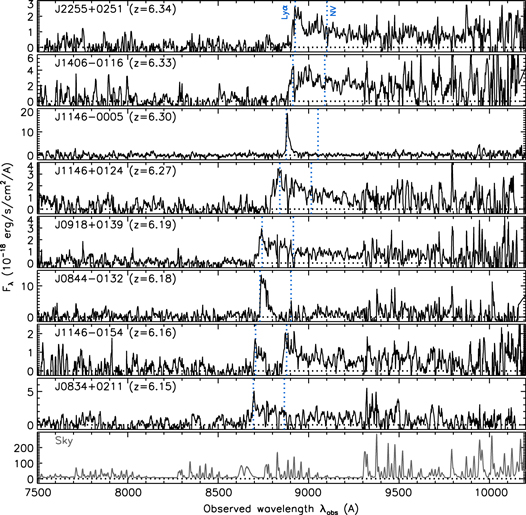
Figure 2. Same as Figure 1, but for the second set of eight quasars.
Download figure:
Standard image High-resolution image
Figure 3. Same as Figure 1, but for the third set of eight quasars.
Download figure:
Standard image High-resolution image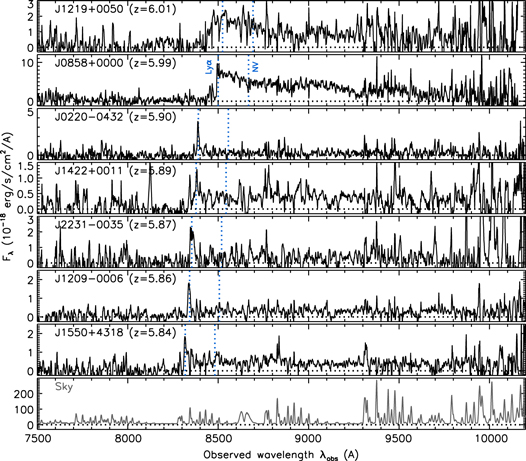
Figure 4. Same as Figure 1, but for the last set of seven quasars.
Download figure:
Standard image High-resolution image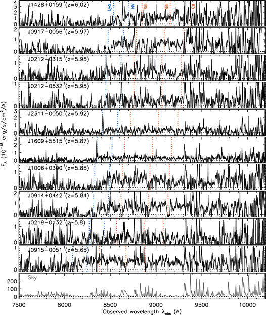
Figure 5. Same as Figure 1, but for the 10 high-z galaxies. The expected positions of the interstellar absorption lines of Si ii λ1260, Si ii λ1304, and C ii λ1335 are marked by the red dotted lines.
Download figure:
Standard image High-resolution image
Figure 6. Same as Figure 1, but for the four [O iii] emitters at z ∼ 0.8. The expected positions of Hγ, Hβ, and two [O iii] lines (λ4959 and λ5007) are marked by the dotted lines.
Download figure:
Standard image High-resolution image
Figure 7. Same as Figure 1, but for the first set of 10 cool dwarfs. The red lines represent the best-fit templates, whose spectral types are indicated in the top left corner of each panel. The small-scale (<100 Å) features seen in the spectra are due to noise, given the low S/N.
Download figure:
Standard image High-resolution image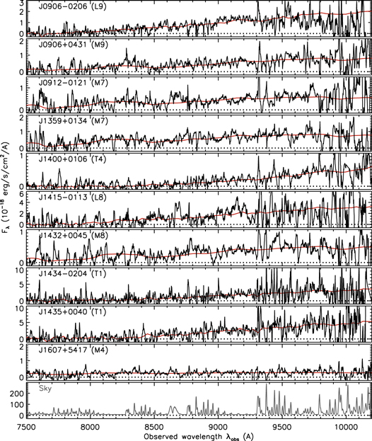
Figure 8. Same as Figure 7, but for the second set of 10 cool dwarfs.
Download figure:
Standard image High-resolution image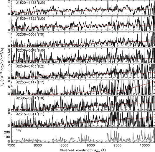
Figure 9. Same as Figure 7, but for the last set of eight cool dwarfs.
Download figure:
Standard image High-resolution imageTable 3. Photometric Properties
| Name | R.A. | Decl. | iAB (mag) | zAB (mag) | yAB (mag) |

|
|---|---|---|---|---|---|---|
| Quasars | ||||||
| J2210+0304 | 22h10m2724 |
+03°04'285 |
27.36 ± 0.78 | >25.03 | 22.94 ± 0.06 | 1.000 |
| J0213−0626 | 02h13m1694 |
−06°26'152 |
26.19 ± 0.30 | >25.05 | 21.69 ± 0.03 | 1.000 |
| J0923+0402 | 09h23m4712 |
+04°02'544 |
26.45 ± 0.24 | 22.64 ± 0.02 | 20.21 ± 0.01 | 1.000 |
| J0921+0007 | 09h21m2056 |
+00°07'229 |
26.28 ± 0.22 | 21.83 ± 0.01 | 21.24 ± 0.01 | 1.000 |
| J1545+4232 | 15h45m0562 |
+42°32'116 |
25.74 ± 0.12 | 22.45 ± 0.01 | 22.16 ± 0.04 | 1.000 |
| J1004+0239 | 10h04m0136 |
+02°39'307 |
26.41 ± 0.11 | 22.76 ± 0.01 | 22.58 ± 0.01 | 1.000 |
| J0211−0203 | 02h11m4453 |
−02°03'039 |
27.47 ± 1.05 | 24.04 ± 0.06 | 23.66 ± 0.10 | 0.999 |
| J2304+0045 | 23h04m2297 |
+00°45'054 |
26.85 ± 0.33 | 23.08 ± 0.02 | 22.75 ± 0.04 | 1.000 |
| J2255+0251 | 22h55m3804 |
+02°51'266 |
>25.72 | 23.44 ± 0.05 | 22.95 ± 0.07 | 1.000 |
| J1406−0116 | 14h06m2912 |
−01°16'112 |
25.78 ± 0.13 | 22.64 ± 0.02 | 21.93 ± 0.03 | 1.000 |
| J1146−0005 | 11h46m5889 |
−00°05'377 |
>26.43 | 23.76 ± 0.04 | 24.78 ± 0.27 | 1.000 |
| J1146+0124 | 11h46m4842 |
+01°24'201 |
26.76 ± 0.42 | 23.01 ± 0.03 | 23.05 ± 0.06 | 1.000 |
| J0918+0139 | 09h18m3317 |
+01°39'233 |
26.70 ± 0.30 | 23.17 ± 0.03 | 23.18 ± 0.04 | 1.000 |
| J0844−0132 | 08h44m0861 |
−01°32'165 |
>26.24 | 23.31 ± 0.03 | 23.73 ± 0.15 | 1.000 |
| J1146−0154 | 11h46m3266 |
−01°54'383 |
26.90 ± 0.55 | 23.60 ± 0.06 | 23.76 ± 0.14 | 1.000 |
| J0834+0211 | 08h34m0088 |
+02°11'469 |
26.27 ± 0.32 | 22.97 ± 0.03 | 22.85 ± 0.05 | 1.000 |
| J0909+0440 | 09h09m2150 |
+04°40'429 |
25.02 ± 0.06 | 22.18 ± 0.02 | 21.91 ± 0.03 | 1.000 |
| J2252+0225 | 22h52m0544 |
+02°25'319 |
26.78 ± 0.37 | 23.80 ± 0.06 | 23.88 ± 0.11 | 1.000 |
| J1406−0144 | 14h06m4688 |
−01°44'026 |
26.78 ± 0.37 | 23.33 ± 0.04 | 23.40 ± 0.13 | 1.000 |
| J1416+0147 | 14h16m5301 |
+01°47'022 |
26.60 ± 0.55 | 22.89 ± 0.04 | 23.46 ± 0.14 | 1.000 |
| J0957+0053 | 09h57m4039 |
+00°53'336 |
>26.91 | 23.66 ± 0.01 | 23.58 ± 0.04 | 1.000 |
| J2223+0326 | 22h23m0951 |
+03°26'203 |
24.07 ± 0.03 | 21.31 ± 0.01 | 21.41 ± 0.02 | 1.000 |
| J1400−0125 | 14h00m2999 |
−01°25'210 |
25.16 ± 0.08 | 22.88 ± 0.02 | 22.82 ± 0.06 | 1.000 |
| J1400−0011 | 14h00m2879 |
−00°11'515 |
26.15 ± 0.19 | 23.62 ± 0.04 | 24.16 ± 0.18 | 1.000 |
| J1219+0050 | 12h19m0534 |
+00°50'375 |
24.90 ± 0.05 | 22.81 ± 0.02 | 23.13 ± 0.06 | 1.000 |
| J0858+0000 | 08h58m1351 |
+00°00'571 |
24.28 ± 0.04 | 21.29 ± 0.01 | 21.43 ± 0.01 | 1.000 |
| J0220−0432 | 02h20m2972 |
−04°32'040 |
26.29 ± 0.18 | 24.42 ± 0.10 | 24.01 ± 0.11 | 0.000 |
| J1422+0011 | 14h22m0023 |
+00°11'030 |
26.22 ± 0.14 | 23.85 ± 0.05 | 23.56 ± 0.08 | 1.000 |
| J2231−0035 | 22h31m4889 |
−00°35'475 |
26.52 ± 0.24 | 24.27 ± 0.07 | 24.35 ± 0.18 | 1.000 |
| J1209−0006 | 12h09m2399 |
−00°06'465 |
26.69 ± 0.23 | 24.13 ± 0.05 | 24.13 ± 0.12 | 1.000 |
| J1550+4318 | 15h50m0093 |
+43°18'028 |
25.52 ± 0.08 | 23.71 ± 0.03 | 23.54 ± 0.10 | 1.000 |
| Galaxies | ||||||
| J1428+0159 | 14h28m2471 |
+01°59'344 |
26.05 ± 0.43 | 22.90 ± 0.05 | 22.83 ± 0.07 | 1.000 |
| J0917−0056 | 09h17m0028 |
−00°56'581 |
26.06 ± 0.18 | 23.69 ± 0.05 | 23.81 ± 0.10 | 1.000 |
| J0212−0315 | 02h12m3667 |
−03°15'176 |
26.98 ± 0.50 | 23.85 ± 0.05 | 23.90 ± 0.13 | 1.000 |
| J0212−0532 | 02h12m4946 |
−05°32'380 |
>26.22 | 24.40 ± 0.08 | 24.31 ± 0.19 | 1.000 |
| J2311−0050 | 23h11m4286 |
−00°50'207 |
26.83 ± 0.41 | 24.23 ± 0.09 | 23.91 ± 0.20 | 0.356 |
| J1609+5515 | 16h09m5279 |
+55°15'485 |
25.89 ± 0.08 | 24.15 ± 0.03 | 24.20 ± 0.09 | 1.000 |
| J1006+0300 | 10h06m3353 |
+03°00'052 |
25.79 ± 0.10 | 23.70 ± 0.02 | 23.65 ± 0.05 | 1.000 |
| J0914+0442 | 09h14m3647 |
+04°42'317 |
25.46 ± 0.12 | 23.29 ± 0.06 | 23.07 ± 0.08 | 0.980 |
| J0219−0132 | 02h19m3094 |
−01°32'072 |
25.47 ± 0.24 | 24.27 ± 0.07 | 24.36 ± 0.13 | 0.820 |
| J0915−0051 | 09h15m4502 |
−00°51'360 |
25.61 ± 0.13 | 24.04 ± 0.08 | 24.19 ± 0.15 | 0.316 |
| [O iii] Emitters | ||||||
| J1000+0211 | 10h00m1246 |
+02°11'274 |
24.65 ± 0.04 | 22.87 ± 0.02 | 25.16 ± 0.28 | 1.000 |
| J0154−0116 | 01h54m3169 |
−01°16'195 |
>23.08 | 22.75 ± 0.04 | 23.19 ± 0.07 | 1.000 |
| J2226+0237 | 22h26m4968 |
+02°37'540 |
24.25 ± 0.03 | 22.61 ± 0.02 | 24.57 ± 0.24 | 1.000 |
| J0845−0123 | 08h45m1654 |
−01°23'216 |
23.59 ± 0.02 | 21.89 ± 0.01 | 24.31 ± 0.19 | 1.000 |
| Cool Dwarfs | ||||||
| J0158−0033 | 01h58m0710 |
−00°33'321 |
>23.65 | 23.80 ± 0.07 | 23.68 ± 0.07 | 0.119 |
| J0207−0052 | 02h07m0105 |
−00°52'250 |
25.34 ± 0.32 | 22.22 ± 0.01 | 21.21 ± 0.01 | 0.831 |
| J0213−0334 | 02h13m5082 |
−03°34'452 |
25.99 ± 0.20 | 23.10 ± 0.03 | 22.10 ± 0.03 | 0.105 |
| J0216−0207 | 02h16m1718 |
−02°07'193 |
26.14 ± 0.26 | 23.99 ± 0.06 | 23.18 ± 0.06 | 0.000 |
| J0220−0134 | 02h20m4741 |
−01°34'506 |
25.73 ± 0.31 | 24.41 ± 0.08 | 24.27 ± 0.12 | 0.042 |
| J0225−0351 | 02h25m0018 |
−03°51'468 |
25.33 ± 0.08 | 23.50 ± 0.05 | 22.96 ± 0.05 | 0.000 |
| J0837−0000 | 08h37m1718 |
−00°00'210 |
23.18 ± 0.01 | 20.24 ± 0.01 | 19.11 ± 0.01 | 0.000 |
| J0856+0248 | 08h56m0910 |
+02°48'511 |
24.63 ± 0.12 | 23.24 ± 0.03 | 22.79 ± 0.05 | 0.000 |
| J0900+0424 | 09h00m1840 |
+04°24'155 |
27.46 ± 0.45 | 24.11 ± 0.08 | 23.21 ± 0.08 | 0.021 |
| J0902−0030 | 09h02m2231 |
−00°30'404 |
26.02 ± 0.22 | 24.07 ± 0.05 | 23.55 ± 0.07 | 0.000 |
| J0906−0206 | 09h06m5082 |
−02°06'102 |
25.06 ± 0.14 | 22.93 ± 0.05 | 22.29 ± 0.04 | 0.000 |
| J0906+0431 | 09h06m5510 |
+04°31'319 |
25.05 ± 0.06 | 23.56 ± 0.06 | 23.12 ± 0.08 | 0.000 |
| J0912−0121 | 09h12m1099 |
−01°21'029 |
>25.77 | 23.74 ± 0.07 | 23.17 ± 0.07 | 0.994 |
| J1359+0134 | 13h59m4500 |
+01°34'123 |
24.60 ± 0.07 | 23.32 ± 0.06 | 23.31 ± 0.10 | 0.533 |
| J1400+0106 | 14h00m1538 |
+01°06'237 |
27.91 ± 0.85 | 25.10 ± 0.15 | 23.50 ± 0.07 | 0.000 |
| J1415−0113 | 14h15m3220 |
−01°13'143 |
25.08 ± 0.06 | 22.30 ± 0.01 | 21.22 ± 0.01 | 0.000 |
| J1432+0045 | 14h32m0578 |
+00°45'317 |
25.59 ± 0.12 | 24.01 ± 0.07 | 23.89 ± 0.11 | 0.027 |
| J1434−0204 | 14h34m3736 |
−02°04'167 |
25.33 ± 0.18 | 22.36 ± 0.03 | 21.42 ± 0.02 | 0.000 |
| J1435+0040 | 14h35m2969 |
+00°40'353 |
25.17 ± 0.06 | 22.12 ± 0.01 | 21.02 ± 0.01 | 0.000 |
| J1607+5417 | 16h07m3284 |
+54°17'245 |
26.46 ± 0.12 | 24.23 ± 0.03 | 23.63 ± 0.05 | 0.295 |
| J1620+4438 | 16h20m4691 |
+44°38'397 |
25.64 ± 0.16 | 23.39 ± 0.09 | 23.16 ± 0.10 | 0.154 |
| J1629+4233 | 16h29m4812 |
+42°33'385 |
25.77 ± 0.09 | 23.72 ± 0.04 | 23.55 ± 0.08 | 1.000 |
| J2236+0006 | 22h36m1242 |
+00°06'326 |
26.27 ± 0.18 | 24.77 ± 0.13 | 24.27 ± 0.18 | 0.000 |
| J2239−0048 | 22h39m5343 |
−00°48'026 |
24.23 ± 0.08 | 23.00 ± 0.04 | 22.55 ± 0.05 | 0.000 |
| J2248+0103 | 22h48m3469 |
+01°03'122 |
26.73 ± 0.38 | 23.63 ± 0.04 | 22.93 ± 0.04 | 0.997 |
| J2253−0117 | 22h53m5780 |
−01°17'053 |
25.65 ± 0.21 | 23.01 ± 0.08 | 22.42 ± 0.04 | 0.347 |
| J2305−0051 | 23h05m0575 |
−00°51'326 |
25.71 ± 0.13 | 23.58 ± 0.09 | 23.47 ± 0.10 | 0.719 |
| J2315−0041 | 23h15m1406 |
−00°41'011 |
25.69 ± 0.13 | 22.72 ± 0.02 | 21.63 ± 0.02 | 0.195 |
Note. Coordinates are at J2000.0. We took magnitudes from the latest HSC-SSP data release, and recalculated PQB for objects selected with the older data releases (this is why the quasar J0220−0432 has  , which used to be higher in the old data release; see the text). Magnitude upper limits are placed at 5σ significance.
Table 4. JHK Magnitudes of the Objects Detected in UKIDSS or VIKING
| UKIDSS | VIKING | |||||
|---|---|---|---|---|---|---|
| Name | JAB | HAB | KAB | JAB | HAB | KAB |
| (mag) | (mag) | (mag) | (mag) | (mag) | (mag) | |
| Quasars | ||||||
| J0923+0402 | 20.02 ± 0.09 | 19.74 ± 0.16 | 19.32 ± 0.09 | ⋯ | ⋯ | ⋯ |
| J0921+0007 | 20.90 ± 0.26 | ⋯ | ⋯ | 21.05 ± 0.15 | ⋯ | 20.38 ± 0.13 |
| J1406−0116 | ⋯ | ⋯ | ⋯ | 22.06 ± 0.24 | ⋯ | ⋯ |
| J0858+0000 | ⋯ | ⋯ | ⋯ | 21.19 ± 0.20 | 21.15 ± 0.20 | 21.18 ± 0.24 |
| Cool Dwarfs | ||||||
| J0837−0000 | ⋯ | ⋯ | ⋯ | 17.87 ± 0.01 | 17.63 ± 0.01 | 17.72 ± 0.01 |
| J0906−0206 | ⋯ | ⋯ | 20.35 ± 0.22 | ⋯ | ⋯ | ⋯ |
| J0912−0121 | ⋯ | ⋯ | ⋯ | ⋯ | ⋯ | 21.55 ± 0.31 |
| J1415−0113 | 19.87 ± 0.16 | 19.67 ± 0.13 | 20.11 ± 0.21 | 20.07 ± 0.08 | ⋯ | 19.71 ± 0.08 |
| J1434−0204 | 20.17 ± 0.19 | ⋯ | ⋯ | 20.44 ± 0.06 | 20.18 ± 0.10 | 20.19 ± 0.08 |
| J1435+0040 | 19.75 ± 0.11 | 19.84 ± 0.13 | 19.86 ± 0.15 | 19.85 ± 0.03 | 19.68 ± 0.06 | 19.87 ± 0.06 |
Download table as: ASCIITypeset image
We identified 31 new quasars at 5.8 < z ≤ 6.9, as displayed in Figures 1–4 and listed in the first section of Table 5. The two highest-z quasars, J2210+0304 and J0213−0626 at z = 6.9 and z = 6.72, respectively, are observed as complete z-band dropouts on the HSC images. J0923+0402 has a very red z − y color, but is clearly visible in the z-band. All the remaining quasars are i-band dropouts. It is worth mentioning that we discovered two quasars at z ∼ 6.5 (J0921+0007 and J1545+4232), where quasars have similar optical colors to Galactic brown dwarfs and are thus hard to identify (see Figure 1 of Paper II). These two quasars have very strong Lyα + N v λ1240 lines, which allowed us to separate them from brown dwarfs due to their unusually blue z − y colors.
Table 5. Spectroscopic Properties
| Name | Redshift | M1450 | Line | EWrest | FWHM | log L |
|---|---|---|---|---|---|---|
| (mag) | (Å) | (km s−1) | (L in erg s−1) | |||
| Quasars | ||||||
| J2210+0304 | 6.9 | −24.44 ± 0.06 | ⋯ | ⋯ | ⋯ | ⋯ |
| J0213−0626 | 6.72 | −25.24 ± 0.02 | Lyα | 16 ± 1 | 1200 ± 100 | 44.18 ± 0.02 |
| J0923+0402 | 6.6 | −26.18 ± 0.14 | ⋯ | ⋯ | ⋯ | ⋯ |
| J0921+0007 | 6.56 | −24.79 ± 0.10 | Lyα | 170 ± 20 | 1400 ± 100 | 45.04 ± 0.01 |
| J1545+4232 | 6.50 | −24.15 ± 0.21 | Lyα | 140 ± 30 | 960 ± 660 | 44.68 ± 0.03 |
| J1004+0239 | 6.41 | −24.52 ± 0.03 | Lyα | 37 ± 2 | 2100 ± 300 | 44.27 ± 0.01 |
| J0211−0203 | 6.37 | −23.36 ± 0.06 | Lyα | 26 ± 3 | 1200 ± 900 | 43.64 ± 0.04 |
| J2304+0045 | 6.36 | −24.28 ± 0.03 | Lyα | 15 ± 1 | 710 ± 40 | 43.79 ± 0.03 |
| J2255+0251 | 6.34 | −23.87 ± 0.04 | Lyα | 19 ± 2 | 1600 ± 300 | 43.72 ± 0.04 |
| J1406−0116 | 6.33 | −24.96 ± 0.06 | ⋯ | ⋯ | ⋯ | ⋯ |
| J1146−0005 | 6.30 | −21.46 ± 0.63 | Lyα | 260 ± 50 | 330 ± 100 | 44.18 ± 0.02 |
| J1146+0124 | 6.27 | −23.71 ± 0.07 | Lyα | 57 ± 6 | 9700 ± 3700 | 44.12 ± 0.03 |
| J0918+0139 | 6.19 | −23.71 ± 0.04 | Lyα | 23 ± 2 | 6200 ± 1700 | 43.74 ± 0.04 |
| J0844−0132 | 6.18 | −23.97 ± 0.11 | Lyα | 57 ± 6 | 1600 ± 300 | 44.25 ± 0.02 |
| J1146−0154 | 6.16 | −23.43 ± 0.07 | Lyα | 7.3 ± 4.0 | 1600 ± 400 | 43.13 ± 0.23 |
| J0834+0211 | 6.15 | −24.05 ± 0.09 | Lyα | 16 ± 4 | 4900 ± 800 | 43.72 ± 0.10 |
| J0909+0440 | 6.15 | −24.88 ± 0.02 | ⋯ | ⋯ | ⋯ | ⋯ |
| J2252+0225 | 6.12 | −22.74 ± 0.06 | Lyα | 47 ± 5 | 2200 ± 600 | 43.65 ± 0.04 |
| J1406−0144 | 6.10 | −23.37 ± 0.16 | Lyα | 68 ± 8 | 1600 ± 500 | 44.00 ± 0.03 |
| J1416+0147 | 6.07 | −23.27 ± 0.10 | Lyα | 68 ± 7 | 2300 ± 200 | 44.03 ± 0.03 |
| J0957+0053 | 6.05 | −22.98 ± 0.04 | Lyα | 26 ± 4 | 2200 ± 1500 | 43.48 ± 0.06 |
| J2223+0326 | 6.05 | −25.20 ± 0.02 | Lyα | 37 ± 2 | 4700 ± 3500 | 44.53 ± 0.02 |
| J1400−0125 | 6.04 | −23.70 ± 0.05 | Lyα | 28 ± 4 | 12000 ± 4000 | 43.80 ± 0.05 |
| J1400−0011 | 6.04 | −22.95 ± 0.11 | Lyα | 56 ± 3 | 620 ± 60 | 43.84 ± 0.01 |
| J1219+0050 | 6.01 | −23.85 ± 0.05 | Lyα | 26 ± 4 | 7500 ± 4400 | 43.84 ± 0.06 |
| J0858+0000 | 5.99 | −25.28 ± 0.01 | Lyα | 24 ± 1 | 11000 ± 1000 | 44.38 ± 0.01 |
| J0220−0432 | 5.90 | −22.17 ± 0.10 | Lyα | 29 ± 2 | < 230 | 43.15 ± 0.03 |
| J1422+0011 | 5.89 | −22.79 ± 0.07 | Lyα | 7.2 ± 1.7 | 980 ± 360 | 42.82 ± 0.10 |
| J2231−0035 | 5.87 | −22.67 ± 0.10 | Lyα | 21 ± 3 | 790 ± 250 | 43.23 ± 0.05 |
| J1209−0006 | 5.86 | −22.51 ± 0.05 | Lyα | 26 ± 5 | 580 ± 50 | 43.01 ± 0.04 |
| J1550+4318 | 5.84 | −22.86 ± 0.04 | Lyα | 4.8 ± 1.5 | 2600 ± 100 | 42.70 ± 0.13 |
| Galaxies | ||||||
| J1428+0159 | 6.02 | −24.30 ± 0.07 | ⋯ | ⋯ | ⋯ | ⋯ |
| J0917−0056 | 5.97 | −23.60 ± 0.07 | ⋯ | ⋯ | ⋯ | ⋯ |
| J0212−0315 | 5.95 | −22.85 ± 0.06 | Lyα | 5.0 ± 1.0 | 650 ± 50 | 42.69 ± 0.09 |
| J0212−0532 | 5.95 | −22.42 ± 0.07 | ⋯ | ⋯ | ⋯ | ⋯ |
| J2311−0050 | 5.92 | −22.72 ± 0.09 | Lyα | 10 ± 1 | 250 ± 90 | 42.89 ± 0.04 |
| J1609+5515 | 5.87 | −22.41 ± 0.04 | Lyα | 9.1 ± 0.6 | 480 ± 260 | 42.81 ± 0.03 |
| J1006+0300 | 5.85 | −22.98 ± 0.05 | ⋯ | ⋯ | ⋯ | ⋯ |
| J0914+0442 | 5.84 | −23.79 ± 0.04 | ⋯ | ⋯ | ⋯ | ⋯ |
| J0219−0132 | 5.8 | −22.25 ± 0.12 | ⋯ | ⋯ | ⋯ | ⋯ |
| J0915−0051 | 5.65 | −22.60 ± 0.03 | ⋯ | ⋯ | ⋯ | ⋯ |
| [O iii] Emitters | ||||||
| J1000+0211 | 0.828 | ⋯ | Hγ | 370 ± 120 | < 230 | 41.67 ± 0.03 |
| ⋯ | Hβ | 860 ± 290 | <230 | 42.04 ± 0.03 | ||
| ⋯ | [O iii] λ4959 | 2000 ± 700 | <230 | 42.41 ± 0.01 | ||
| ⋯ | [O iii] λ5007 | 6000 ± 2000 | <230 | 42.88 ± 0.01 | ||
| J0154−0116 | 0.808 | ⋯ | Hγ | 58 ± 14 | 410 ± 290 | 41.23 ± 0.10 |
| ⋯ | Hβ | 85 ± 13 | <230 | 41.39 ± 0.05 | ||
| ⋯ | [O iii] λ4959 | 130 ± 18 | 240 ± 140 | 41.57 ± 0.04 | ||
| ⋯ | [O iii] λ5007 | 320 ± 30 | <230 | 41.96 ± 0.02 | ||
| J2226+0237 | 0.805 | ⋯ | Hγ | 120 ± 20 | 390 ± 40 | 41.50 ± 0.05 |
| ⋯ | Hβ | 270 ± 50 | 270 ± 50 | 41.86 ± 0.03 | ||
| ⋯ | [O iii] λ4959 | 480 ± 80 | <230 | 42.11 ± 0.01 | ||
| ⋯ | [O iii] λ5007 | 1400 ± 200 | <230 | 42.59 ± 0.01 | ||
| J0845−0123 | 0.728 | ⋯ | Hγ | ⋯ | ⋯ | ⋯ |
| ⋯ | Hβ | 680 ± 70 | <230 | 42.52 ± 0.01 | ||
| ⋯ | [O iii] λ4959 | 1600 ± 200 | <230 | 42.89 ± 0.01 | ||
| ⋯ | [O iii] λ5007 | 4700 ± 500 | <230 | 43.37 ± 0.01 | ||
Note. Redshifts are recorded to two significant figures when the position of Lyα emission or interstellar absorption is unambiguous.
Download table as: ASCIITypeset image
The majority of the objects in Figures 1–4 exhibit characteristic spectral features of high-z quasars, namely strong and broad Lyα and in some cases N v λ 1240, blue rest-UV continua, and sharp continuum breaks just blueward of Lyα. However, for some objects, the quality and wavelength coverage of our spectra are not sufficient to provide robust classification. In Papers I and II, we reported objects with luminous and narrow Lyα emission, whose quasar/galaxy classification is still ambiguous. Our new quasar sample also includes two such objects, namely J0220−0432 and J1209−0006. Following Papers I and II, we classify these objects as possible quasars, due to their high Lyα luminosity (L > 1043 erg s−1). This is based on the fact that, at z ∼ 2, the majority of Lyα emitters with L > 1043 erg s−1 are associated with AGNs, based on their X-ray, UV, and radio properties (Konno et al. 2016).
We estimated the redshifts of the discovered quasars from the Lyα lines, assuming that the observed line peaks correspond to the intrinsic Lyα wavelength (1216 Å in the rest-frame). This assumption is not always correct, due to the strong H i absorption from the IGM. It is more difficult to measure redshifts of quasars without clear Lyα lines, as is the case for J2210+0304, J0923+0402, and several other quasars in our sample. In these cases we estimated rough redshifts from the wavelengths of the onset of the Gunn–Peterson trough. Therefore, the redshifts presented here (Table 5) are accompanied by relatively large uncertainties (up to Δz ∼ 0.1), and must be interpreted with caution. Future follow-up observations at other wavelengths, e.g., near-IR covering Mg ii λ2800 or sub-mm covering [C ii] 158 μm, are crucial for secure redshift measurements.
The absolute magnitude M1450 and Lyα line properties were measured in the same way as described in Paper II. For every object, we defined a continuum window at wavelengths relatively free from strong sky emission lines, and extrapolated the measured continuum flux to estimate M1450. A power-law continuum model with a slope α = −1.5 (Fλ ∝ λα; e.g., Vanden Berk et al. 2001) was assumed. Since the continuum windows (falling in the range of λrest = 1250–1350 Å) are close to λrest = 1450 Å, these measurements are not sensitive to the exact value of α. The Lyα properties (luminosity, FWHM, and rest-frame equivalent width [EW]) of an object with weak continuum emission, such as J1146−0005, were measured with a local continuum defined as an average flux of all the pixels redward of Lyα. For the remaining objects with relatively strong continuum, we measured the properties of the broad Lyα + N v complex, with a local continuum defined by the above power-law model. We did not assume any line profile models, but used the continuum-subtracted flux counts directly to measure these line properties. Due to the difficulty in defining accurate continuum levels, these line measurements should be regarded as only approximate. The resultant line properties are summarized in Table 5. More detailed descriptions of the above procedure may be found in Paper II.
The 10 objects without a broad or luminous (>1043 erg s−1) Lyα line, as presented in Figure 5, are most likely galaxies at z ∼ 6. We have now spectroscopically identified 24 such high-z luminous galaxies, when combined with the similar objects presented in the previous papers. The redshifts of these objects were estimated from the observed positions of Lyα emission, the interstellar absorption lines of Si ii λ1260, Si ii λ1304, C ii λ1335, and/or the continuum break caused by the IGM H i absorption. This is not always easy with our limited S/N, hence the redshifts reported here must be regarded as only approximate (with uncertainties up to Δz ∼ 0.1). The absolute magnitude M1450 and Lyα properties were measured in the same way as for quasars, except that we assumed a continuum slope of β = −2.0 (Fλ ∝ λβ; Stanway et al. 2005).
This paper also adds four [O iii] emitters at z ∼ 0.8 (see Figures 6) to the two similar objects reported in Paper II. We measured the line properties of Hγ, Hβ, [O iii] λ4959 and λ5007, and listed the results in Table 5. Since they have very weak continua, we estimated the continuum levels by summing up all the available pixels except for the above emission lines. This still gives relatively large uncertainties in the EWs for some of the objects. As we discussed in Paper II, their very high [O iii] λ5007/Hβ ratios may indicate that these are galaxies with sub-solar metallicity and high ionization state of the interstellar medium (e.g., Kewley et al. 2016), and/or AGN contribution. J1000+0211 and J0845−0123 have extremely large [O iii] λ5007 EWs (≳5000 Å), which even exceeds those found in the so-called "green pea" galaxies characterized by strong [O iii] λ5007 (EW ≲ 1000 Å; Cardamone et al. 2009). These objects could be an interesting subject for future follow-up studies.
Finally, we found 28 new Galactic cool dwarfs (low-mass stars and brown dwarfs), as presented in Figures 7–9. We estimated their rough spectral classes by fitting the spectral standard templates of M4- to T8-type dwarfs, taken from the SpeX Prism Spectral Library (Burgasser 2014; Skrzypek et al. 2015), to the observed spectra at λ = 7500–9800 Å. The results are summarized in Table 6 and plotted in the figures. Due to the low S/N and limited wavelength coverage of the spectra, the classification presented here is accompanied by large uncertainties, and should be regarded as only approximate.
Table 6. Spectral Classes of The Cool Dwarfs
| Name | Class |
|---|---|
| J0158−0033 | M5 |
| J0207−0052 | T2 |
| J0213−0334 | T0 |
| J0216−0207 | L2 |
| J0220−0134 | L2 |
| J0225−0351 | M7 |
| J0837−0000 | L9 |
| J0856+0248 | M9 |
| J0900+0424 | L8 |
| J0902−0030 | M7 |
| J0906−0206 | L9 |
| J0906+0431 | M9 |
| J0912−0121 | M7 |
| J1359+0134 | M7 |
| J1400+0106 | T4 |
| J1415−0113 | L8 |
| J1432+0045 | M8 |
| J1434−0204 | T1 |
| J1435+0040 | T1 |
| J1607+5417 | M4 |
| J1620+4438 | M5 |
| J1629+4233 | M5 |
| J2236+0006 | T0 |
| J2239−0048 | M6 |
| J2248+0103 | L2 |
| J2253−0117 | T7 |
| J2305−0051 | T0 |
| J2315−0041 | T1 |
Note. These classifications should be regarded as only approximate; see the text.
Download table as: ASCIITypeset image
In Figure 10, we plot the HSC iAB − zAB and zAB − yAB colors of all the spectroscopically identified objects in Papers I and II and this work. We also include the 10 previously known quasars recovered by SHELLQs. The figure demonstrates that the discovered quasars broadly follow the expected colors from our SED model, while there are outliers with very blue zAB − yAB colors, due to exceptionally large Lyα EWs. On the other hand, we are finding many cool dwarfs that are bluer than our fiducial models, due to the nature of our selection criteria. It may be worth noting a clump of brown dwarfs at (iAB − zAB, zAB − yAB) ∼ (3, 1); they lie exactly on the quasar SED track in the color space, and are thus assigned with high  values as candidates of quasars at z ∼ 6.5. The z ∼ 6 galaxies occupy colors in between quasars and cool dwarfs, due to their weaker Lyα emission than quasars and bluer continua than cool dwarfs. Finally, the six [O iii] emitters are well separated from the quasars on this diagram, and do not satisfy our latest selection condition of iAB − zAB > 2.0.

Figure 10. HSC iAB − zAB and zAB − yAB colors of the SHELLQs quasars (blue dots; including previously known quasars we recovered), galaxies (green dots), [O iii] emitters (light blue dots), and cool dwarfs (red dots). The gray crosses and dots represent Galactic stars (Pickles 1998) and brown dwarfs, while the solid and dashed lines represent models of quasars and galaxies at z ≥ 5.7; the dots along the lines represent redshifts in steps of 0.1, with z = 5.7 marked by the large open circles. The dotted lines represent the color criteria used in our HSC database query. The four quasars in the top left corner (marked by the up arrows) are undetected in the i- and z-bands, and are plotted at arbitrary horizontal positions. All the sources discovered in Papers I and II and this work are included.
Download figure:
Standard image High-resolution imageFigure 11 displays the redshifts versus the absolute magnitudes M1450 of the SHELLQs quasars and galaxies, along with those of high-z quasars discovered by other surveys. We continue to probe a new parameter space at z > 5.7 and M1450 > −25 mag, to which other surveys have only limited sensitivities.
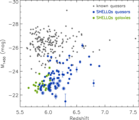
Figure 11. Rest-UV absolute magnitude at 1450 Å (M1450), as a function of redshift, of the SHELLQs quasars (blue dots) and galaxies (green dots), as well as of all the high-z quasars discovered by other surveys and published to date (small gray dots). The SHELLQs quasars with narrow Lyα lines are marked with the larger circles. All the high-z objects discovered in Papers I and II and this work are plotted.
Download figure:
Standard image High-resolution imageFigure 12 presents a histogram of the Bayesian quasar probability ( ), for all the spectroscopically identified objects in Papers I and II and this work. The
  values have a clear bimodal distribution, with the higher peak at
  being dominated by high-z quasars. All but one quasar have
  , which implies that their spectral diversity is reasonably covered by the quasar model in our Bayesian algorithm. The lower peak at
  is populated mostly by cool dwarfs. Many of these dwarfs lie below the quasar selection threshold (
 ), due to the improvement of HSC photometry with updates of the data reduction pipeline; they were selected for spectroscopic identification because they had
  in the older data releases. This is also the case for the quasar J0220−0432, which had zAB − yAB ∼ 0.0 and PQB = 1.0 previously, but happens to have zAB − yAB ∼ 0.4 and
  in the latest data release. Because no additional z- or y-band data were taken for this object since the previous data release, and because this object is located within a few arcseconds of a brighter galaxy, this discrepancy in color measurements may be due to different deblender treatment in the different versions of the HSC pipeline.

Figure 12. Histogram of the Bayesian quasar probability ( ) of the SHELLQs quasars (blue; including previously known quasars we recovered), galaxies (green), [O iii] emitters (light blue), and cool dwarfs (red). All the sources discovered in Papers I and II and this work are counted. The dashed line represents our quasar selection threshold (
 ); there are objects below this threshold, because they had higher
  in the older HSC data releases.
Download figure:
Standard image High-resolution image
5. Summary
This paper is the fourth in a series presenting the results from the SHELLQs project, a search for low-luminosity quasars at z ≳ 6 based on the deep multi-band imaging data produced by the HSC-SSP survey. We continue to use the quasar selection procedure we described in Papers I and II, and here report spectroscopy of additional objects that roughly double the number of identifications compared to previous papers. Through the SHELLQs project, we have so far identified 137 extremely red HSC sources over about 650 deg2, which include 64 high-z quasars, 24 high-z luminous galaxies, 6 [O iii] emitters at z ∼ 0.8, and 43 Galactic cool dwarfs. Our discovery now exceeds, in number, the final SDSS sample of 52 high-z quasars (Jiang et al. 2016). The new quasars span luminosities from M1450 ∼ −26 to −22 mag, and continue to probe luminosities a few magnitudes lower than those probed by previous wide-field surveys. Our companion paper will present the quasar luminosity function established over an unprecedentedly wide range of M1450 ∼ −28 to −21 mag, using the SHELLQs and other survey outcomes.
Our project will continue to identify high-z quasars in the HSC data, as the SSP survey continues toward its goal of observing 1400 deg2 in the Wide layer, and 27 and 3.5 deg2 in the Deep and UltraDeep layers, respectively. At the same time, we are carrying out multi-wavelength follow-up observations of the discovered objects. Black hole masses are being measured with Mg ii λ2800 lines obtained with near-IR spectrographs on Subaru, the Gemini telescopes, and the Very Large Telescope (M. Onoue et al. 2018, in preparation). We are also using ALMA, in order to probe the stellar and gaseous properties of the host galaxies (partly published in Izumi et al. 2018). The results of these observations will be presented in forthcoming papers.
This work is based on data collected at the Subaru Telescope, which is operated by the National Astronomical Observatory of Japan (NAOJ). We appreciate the staff members of the telescope for their support during our FOCAS observations. The data analysis was in part carried out on the open use data analysis computer system at the Astronomy Data Center of NAOJ.
This work is also based on observations made with the Gran Telescopio Canarias (GTC), installed at the Spanish Observatorio del Roque de los Muchachos of the Instituto de Astrofísica de Canarias, on the island of La Palma. We thank Stefan Geier and other support astronomers for their help during preparation and execution of our observing program.
Y.M. was supported by the Japan Society for the Promotion of Science (JSPS) KAKENHI grant No. JP17H04830.
The Hyper Suprime-Cam (HSC) collaboration includes the astronomical communities of Japan and Taiwan, and Princeton University. The HSC instrumentation and software were developed by NAOJ, the Kavli Institute for the Physics and Mathematics of the Universe (Kavli IPMU), the University of Tokyo, the High Energy Accelerator Research Organization (KEK), the Academia Sinica Institute for Astronomy and Astrophysics in Taiwan (ASIAA), and Princeton University. Funding was contributed by the FIRST program from Japanese Cabinet Office, the Ministry of Education, Culture, Sports, Science and Technology (MEXT), the Japan Society for the Promotion of Science (JSPS), Japan Science and Technology Agency (JST), the Toray Science Foundation, NAOJ, Kavli IPMU, KEK, ASIAA, and Princeton University.
This paper makes use of software developed for the Large Synoptic Survey Telescope (LSST). We thank the LSST Project for making their code available as free software at http://dm.lsst.org.
The Pan-STARRS1 Surveys (PS1) have been made possible through contributions of the Institute for Astronomy, the University of Hawaii, the Pan-STARRS Project Office, the Max-Planck Society and its participating institutes, the Max Planck Institute for Astronomy, Heidelberg and the Max Planck Institute for Extraterrestrial Physics, Garching, The Johns Hopkins University, Durham University, the University of Edinburgh, Queen's University Belfast, the Harvard-Smithsonian Center for Astrophysics, the Las Cumbres Observatory Global Telescope Network Incorporated, the National Central University of Taiwan, the Space Telescope Science Institute, the National Aeronautics and Space Administration under Grant No. NNX08AR22G issued through the Planetary Science Division of the NASA Science Mission Directorate, the National Science Foundation under Grant No. AST-1238877, the University of Maryland, Eötvös Lorand University (ELTE), and the Los Alamos National Laboratory.
IRAF is distributed by the National Optical Astronomy Observatory, which is operated by the Association of Universities for Research in Astronomy (AURA) under a cooperative agreement with the National Science Foundation.
Footnotes
- 24
Throughout this paper, "high-z" denotes z > 5.7, where quasars are observed as i-band dropouts in the Sloan Digital Sky Survey (SDSS) filter system (Fukugita et al. 1996). The term "X-band dropouts" or "X-dropouts" refers to objects that are much fainter in the X and bluer bands (and very often invisible) than in the redder bands.
- 25
- 26