


Abstract
We present Breakthrough Listen's Exotica Catalog as the centerpiece of our efforts to expand the diversity of targets surveyed in the Search for Extraterrestrial Intelligence (SETI). As motivation, we introduce the concept of survey breadth, the diversity of objects observed during a program. Several reasons for pursuing a broad program are given, including increasing the chance of a positive result in SETI, commensal astrophysics, and characterizing systematics. The Exotica Catalog is a 963 entry collection of 816 distinct targets intended to include "one of everything" in astronomy. It contains four samples: the Prototype sample, with an archetype of every known major type of nontransient celestial object; the Superlative sample of objects, with the most extreme properties; the Anomaly sample of enigmatic targets that are in some way unexplained; and the Control sample, with sources not expected to produce positive results. As far as we are aware, this is the first object list in recent times with the purpose of spanning the breadth of astrophysics. We share it with the community in hopes that it can guide treasury surveys and as a general reference work. Accompanying the catalog is an extensive discussion of the classification of objects and a new classification system for anomalies. Extensive notes on the objects in the catalog are available online. We discuss how we intend to proceed with observations in the catalog, contrast it with our extant Exotica efforts, and suggest how similar tactics may be applied to other programs.
Export citation and abstract BibTeX RIS
1. Introduction
Breakthrough Listen is a 10 year program to conduct the deepest surveys for extraterrestrial intelligence (ETI) in the radio and optical domains (Worden et al. 2017). The core of the program is a deep search for artificial radio emission from over a thousand nearby stars and galaxies (Isaacson et al. 2017, hereafter I17; see also Enriquez et al. 2017; Price et al. 2020 for results) and commensal studies of a million more stars in the Galaxy (Worden et al. 2017). It joins other programs in the Search for Extraterrestrial Intelligence (SETI), most of which have also focused on nearby stars (Tarter 2001). But where should we look for ETIs? Indeed, how should we look for new phenomena of any kind?
Serendipity is a key ingredient in the discovery of most new types of phenomena and extraordinary new objects (Harwit 1981; Dick 2013; Wilkinson 2016). From Ceres 11 to pulsars, from the cosmic microwave background (CMB) to gamma-ray bursts (GRBs), the majority of unknown phenomena have been found by observers that were not explicitly looking for them. 12 Historically, theory has rarely driven these findings. 13 Instead, they frequently come about through new regions of parameter space being opened by new instruments and telescopes (Harwit 1981).
Other discoveries—like the moons of Mars or Cepheid variables in external galaxies—were delayed because no thorough observations were carried out on the targets (Hall 1878; Dick 2013). The pattern persists to this day. Because ultracompact dwarf galaxies have characteristics that fall in the cracks between other galaxies and globular clusters, they were only recognized recently despite being easily visible on images for decades (Phillipps et al. 2001; Sandoval et al. 2015). Of relevance to SETI, hot Jupiters were speculated about in the 1950s (Struve 1952), but they were not discovered until 1995 in part because no one systematically looked for them (for further context, see Mayor & Queloz 2012; Walker 2012; Cenadelli & Bernagozzi 2015). This may have delayed by years the understanding that exoplanets are not extremely rare, one of the factors in the widely used Drake Equation in SETI relating the number of ETIs to evolutionary probabilities and their lifespan (Drake 1962).
Despite searches spanning several decades, no compelling evidence for ETIs has been found by the SETI community to date (e.g., Horowitz & Sagan 1993; Griffith et al. 2015; Lipman et al. 2019; Pinchuk et al. 2019; Price et al. 2020; Sheikh et al. 2020). The continuing lack of a discovery among SETI efforts looking for various technosignatures is sometimes called the Great Silence (Brin 1983). If at least some ETIs are willing and capable of expanding across interstellar space, a bolder interpretation of the null results is popularly referred to as the Fermi Paradox, the unexpected lack of any obvious technosignatures in the solar system (Ćirković 2009). 14 Although the simplest resolution may be that we are alone in the local universe (Hart 1975; Wesson 1990), and others question whether we should expect to have detected technosignatures yet (Tarter 2001; Wright et al. 2018), many have suggested that ETIs are actually abundant but we are simply looking in the wrong places for them (e.g., Corbet 1997; Ćirković & Bradbury 2006; Davies 2010; Di Stefano & Ray 2016; Benford 2019; Gertz 2019). It is very difficult to detect a society of similar power and technology to our own through the traditional methods of narrowband radio searches unless it makes intentional broadcasts (Forgan & Nichol 2011). But like hot Jupiters, might there be easy discoveries in SETI that we keep missing because we keep looking in the wrong ways or at the wrong places?
Considerations like these in astrophysics have inspired efforts to accelerate serendipity by expanding the region of parameter space explored by instruments (see Harwit 1981; Djorgovski et al. 2001; Cordes & International SKA Science Working Group 2006; Djorgovski et al. 2013). 15 Zwicky (1957) advocated a philosophy of "morphological astronomy" in which essentially all possible phenomena are considered and more specifically searching unexplored regions of parameter space to counter biases. 16 This approach has been highlighted in SETI to gauge the progress of the search (Wright et al. 2018; Davenport 2019; see also Sheikh 2020). 17 Breakthrough Listen harnesses expanding capabilities in several dimensions. In radio, Breakthrough Listen has developed a unique backend, already implemented on the Green Bank Telescope (MacMahon et al. 2018) and the CSIRO Parkes telescope (Price et al. 2018), and more are being installed on MeerKAT (an array described in Jonas 2009). These allow for an unprecedented frequency coverage at high spectral and temporal resolution. In the optical, Breakthrough Listen continues to use the Automated Planet Finder (APF; Vogt et al. 2014) for high-spectral-resolution observations of stars in hopes of spotting laser emission (e.g., Lipman et al. 2019), and we have partnered with the VERITAS gamma-ray telescope (Very Energetic Radiation Imaging Telescope Array System; Weekes et al. 2002) for its sensitivity to extremely short optical pulses (Abeysekara et al. 2016). But we can also consider exploring observational parameter space, too, by expanding our strategies for where and when to look.
This paper presents our motivations and initial selection and strategies for exotic targets. The centerpiece is a broad catalog of targets, most of them unlike those previously covered by SETI, that we intend to observe over the coming years. Although I17 already included a broad range of stellar and galaxy types, the Exotica Catalog's aim is to include "one of everything" to ensure that we are not missing some obvious technosignatures. Also among the targets are extreme examples of cosmic phenomena, to cover the full range of environments, and mysterious anomalies that might yield interesting results if examined closely. In addition, we describe our other efforts to expand SETI in unconventional directions and to enhance our primary scientific results with campaigns observing selected classes of interesting targets. In these efforts, we seek evidence for both ETIs and new astrophysical phenomena.
We present this catalog in hope that it aids in other searches for unexpected phenomena. A program of observing as wide a range of targets as possible does not need to be restricted to SETI, or to radio and optical wavelengths. Any new facility across the spectrum might benefit by doing a treasury survey using a catalog based off or inspired by this one. We also hope that the catalog is useful as a reference for educational purposes or for early researchers by providing a convenient summary to what is currently known to be "out there" with references. Online notes provide further details on the entries, target selection, and further references.
The paper has the following structure. We discuss basic concepts motivating exotica observations and the catalog in Section 2. A brief overview of the division of the catalog into four samples is presented in Section 3. The next four sections each describe the construction and principles behind each of these samples: the Prototype sample in Section 4, the Superlative sample in Section 5, the Anomaly sample in Section 6, and the Control sample in Section 7. We discuss the properties of the Exotica Catalog and its planned supplementary materials in Section 8. Section 9 discusses the need for wide-field surveys to fully span the breadth of astrophysics. We discuss possible strategies for the catalog and other exotica efforts in Section 10. Section 11 is a summary of the paper. A series of appendices presents the entries in each sample: Prototypes in Appendix A, with discussion of classification; Superlatives in Appendix B; Anomalies in Appendix C; and Controls in Appendix D. Appendix E presents the full unified catalog, with notes on data sources used.
2. Concepts
2.1. Breadth, Depth, and Count
Each astronomical survey on a given instrument makes trade-offs. To illustrate the differences of our programs, we distinguish between three measures of the extent of a targeted survey of individual axes. The program must balance the variety of observed object types, the number of each observed type of object, and how long to spend observing each individual object. We call these three dimensions breadth, count, and depth, respectively. These three quantities can be loosely thought of as three different dimensions of parameter space, and a survey searches a bounded volume within that space, as depicted in Figure 1. A program can emphasize extent along one dimension over another, but because of limited observational resources, it cannot cover the entire realm of possibilities.

Figure 1. A cartoon of the three directions of target selection and the relative advantages of Breakthrough Listen's primary programs observing stars and galaxies (green), a survey of the Breakthrough Listen Exotica Catalog (blue), and some example campaigns. Previous SETI surveys have generally aimed for maximal depth, achieving strong limits for a small number of similar targets, or count, achieving modest limits for a large number of similar targets. Other exotica efforts can include high-depth (red) or high-count (gold) campaigns, but observations of the Exotica Catalog will be broad, achieving modest limits on a small number each of a wide variety of targets. Future discoveries may be added to a later version of the catalog (pale blue), or prompt new campaigns that we cannot yet plan for (gray).
Download figure:
Standard image High-resolution imageThe reader should be cautioned, however, that Figure 1 is not literal. Each "dimension" can itself be multivalent (for example, increasing depth by increasing integration time versus cadence versus frequency coverage) and thus could actually be represented as a subspace with many dimensions (as in Harwit 1981; Djorgovski et al. 2013; Wright et al. 2018). Our emphasis here is evaluating the target selection of a survey rather than its effectiveness for a given target (see also Sheikh 2020). Note also that breadth and count apply more to targeted surveys rather than wide-field surveys, which may be better parameterized with sky area (see Djorgovski et al. 2013).
Breadth, count, and depth each emphasize different levels of confidence in our ideas about for where we can make desired discoveries. If we are very confident that a phenomenon, such as ETIs, is very common around a particular kind of object, like G dwarfs, we should push for high depth. Depth is essential when we are sure the signals will be faint, because shallow observations cannot then be successful. If instead we believe that a phenomenon is very rare, but are still sure of the environments that generate it, then we should aim to examine a large number of objects, in hopes that some of its signatures will turn out to be bright. Finally, if we have no idea where we are likely to find a phenomenon, it makes sense to have a broad survey. After all, we do not want to keep missing something otherwise obvious because we never happen to look. Shifting our emphasis from depth to count to breadth allows for increasing levels of serendipity.
The guiding assumption of many previous SETI efforts has been that ETIs are likely to live around Sunlike stars and are not vastly more powerful than our own. This kind of technological society is the only one known to exist (e.g., Sagan et al. 1993), and a conservative approach minimizes the amount of speculation piled upon the hypotheses that ETIs are common and that they broadcast brightly enough to be detected. Some surveys have gone for the deep approach by examining a few nearby stars with high sensitivity (as in Rampadarath et al. 2012). Drake's equation implies that it is unlikely for a given star to be inhabited now, unless the ETIs persist for billions of years or have interstellar travel. For this reason, a common SETI approach is to examine a large number of sunlike stars, as with the HabCat of Project Phoenix (Turnbull & Tarter 2003).
Few SETI surveys have sought to examine a broad range of possible habitats. An important exception to this are the all-sky surveys, as done with Big Ear (Dixon 1985) or META (Horowitz & Sagan 1993). In a way, all-sky surveys allow for the ultimate breadth and count because they observe everything in the sky. Even if a new phenomenon is completely unknown, an all-sky survey has a chance to pick it up. In order to accomplish this, however, they tend to have a very low depth. The limited number of SETI surveys of external galaxies may be considered broad to the extent the target galaxies presumably include all kinds of stellar and planetary phenomena, although the diversity of galaxies itself is usually limited (Shostak et al. 1996; Gray & Mooley 2017). As far as targeted surveys go, Harp et al. (2018) is one of the few recent efforts that emphasize breadth; their targets included quasars, masers, pulsars, supernova remnants, and an Earth–Sun Lagrange point.
Surveys are constrained by the cost and ease of access to facilities. Breakthrough Listen has unprecedented access to powerful instruments for SETI purposes, allowing our program to stretch out in all three directions. Our main efforts so far have concentrated on the nearby stars and galaxies listed in I17. This is a relatively broad catalog in SETI terms, including stars of spectral type from B to M and class from dwarfs to giants, as well as galaxies with a wide range of luminosities and morphologies. Our reach will be expanded immensely by our upcoming million star survey with MeerKAT, a commensal effort that will achieve the largest count of a targeted SETI search. Nonetheless, its breadth is limited because the types sampled are not too rare, unconventional, or extreme: there are no X-ray binaries or blazars in the I17 sample, for example.
To supplement the large but finite extent of I17 (green boxes in Figure 1), we have engaged in several additional programs that can extend along any of the three dimensions. In some cases (yellow boxes), we have effectively appended an object class to I17 by observing a number of examples, as with brown dwarfs (Price et al. 2020). In others, we have focused intently on a single extraordinary object to a high depth (red boxes), as in our studies of the repeating FRB 121102 (Gajjar et al. 2018). To these efforts, we now add the Exotica Catalog (blue box), an effort to cover the full range of known astrophysical phenomena. The broadness of this catalog is unprecedented in targeted SETI, with only all-sky surveys being even broader. Given how little we know about ETI prevalence, forms, technology, and motivations, we believe that efforts along all three dimensions are necessary.
2.2. Core Motivations for an Exotica SETI Program
We have several motivations in mind for observing exotic targets, and these have informed the kind of catalogs we have created:
- 1.Motivation I: constraining the possibility of different kinds of intelligence living in non-Earthly habitats. Speculations about exotic habitats in the literature include life living on habitable icy worlds around red giants (Lorenz et al. 1997; Lopez et al. 2005; Ramirez & Kaltenegger 2016), inside large carbonaceous asteroids (Abramov & Mojzsis 2011), in Kuiper Belts (Dyson 2003), inside rogue planets (Stevenson 1999; Abbot & Switzer 2011), or in the atmospheres of gas giants and brown dwarfs (Sagan & Salpeter 1976; Sagan 1994; Yates et al. 2017). Exotic life may be based on alternate biochemistries (Bains 2004; Baross et al. 2007). Intelligence does not need to be native to unusual habitats, as some locations may draw ETIs from their home worlds for reasons of energy collection, curiosity, or isolation. Some phenomena might be modulated or harnessed to act as beacons (e.g., Cordes 1993; Learned et al. 2008; Chennamangalam et al. 2015). The postbiological universe paradigm also suggests that a spacefaring intelligence could be very different from its biological origins, with very different needs (Scheffer 1994; Dick 2003). The practicality of some kinds of megastructures may depend on their environment or the phenomenon they are harnessing (Semiz & Oğur 2015; Osmanov 2016). Thus, there could be inhabited environments that seem inhospitable to us, like the central engine of an active galactic nucleus (AGN) or the outskirts of a galaxy (some examples include Dyson 1963; Ćirković & Bradbury 2006; Inoue & Yokoo 2011; Vidal 2011; Lingam & Loeb 2020). This goal motivates us to examine a wide variety of phenomena, both typical and extreme examples.
- 2.Motivation II: constraining the possibility that some astrophysical phenomena or objects are themselves artificial, a possibility suggested at least as early as the 1960s by Kardashev (1964). Blue straggler stars and fast radio bursts are examples of classes posited as engineered in the literature (Beech 1990; Lingam & Loeb 2017). It is not just entire source classes, but individual mysterious objects or small subclasses that might be artificial as well. Examples of these anomalies include Boyajian's Star and Przybylsky's Star (Wright et al. 2016) and Hoag's Object (Voros 2014). Although nonartificial explanations are far likelier and frequently plentiful, there is a small chance that we are throwing away evidence of ETIs that is staring us in the face because it does not fit our preconceptions (e.g., Ćirković 2018). This goal motivates us to examine rare, unusual subtypes of astronomical phenomena, as well as anomalous sources that defy explanation.
- 3.Motivation III: constraining the possibility that some natural phenomena mimic ETIs. 18 Pulsars were briefly if unseriously considered possible contenders for alien signals because of their regular radio signals (for a historical perspective on the SETI context, see Penny 2013). The Astropulse survey seeks nanosecond-long radio pulses from ETIs (Siemion et al. 2010), but brief pulses are known to be generated by the Crab Pulsar (Hankins et al. 2003), and it is possible that evaporating primordial black holes and relativistic fireballs produce similar signals (Rees 1977; Thompson 2017). Thus, we want to deliberately seek out objects that are likely to generate unusual signals naturally. This goal motivates us to examine extreme objects and those with nonthermal emission mechanisms.
- 4.Motivation IV: using the unique Breakthrough Listen instrumentation for general astrophysical interest. Previous efforts along these lines include our observations of fast radio bursts (Gajjar et al. 2018; Price et al. 2019a). This goal motivates us to examine a wide range of sources, not just stars and galaxies that are hospitable to life.
- 5.Motivation V: constraining the possibility that some unexpected systematics generate false positives for ETIs. These might include instrumental problems, problems with analysis, or especially radio frequency interference (RFI). A claimed detection of an ETI, or even an unusual natural phenomenon, will lead to considerable skepticism. By conducting observations where we expect nothing at all, we learn about the behavior of the instrument system. This goal motivates us to examine empty spots on the sky, or unphysical "sources" like the zenith.
2.3. Campaigns and Catalogs
Previously we have focused on targets classes that are typical of SETI, for which the nearest members were well known. In contrast, exotica include the more dynamic side of astrophysics. The list of known astrophysical phenomena, and proposed links between them and ETIs, is always growing. Some of the phenomena that fall under the auspice of exotica include violent and energetic objects that emit bright transients, like pulsars and AGNs. Others are very faint or small, so faint that new nearby examples are constantly being discovered, like the coolest brown dwarfs and ultrafaint galaxies. Either way, a program that observes exotica for SETI reasons needs to be more flexible than one that observes nearby stars and galaxies.
Breakthrough Listen has two basic approaches to observe exotic objects. The first is a series of short campaigns, each dedicated to a particular object or object class. If someone proposes a phenomenon is actually artificial or claims detection of ETIs, we follow up on it by observing it. By focusing on just a few objects each, these campaigns allow us to peer deeply to lower flux levels, constraining transmitters with lower equivalent isotropic radiated power (EIRP). 19 Unlike the catalogs of stars and galaxies, these programs are developed as new opportunities and discoveries arise, a more dynamic approach than having a fixed catalog. Some examples are discussed in Section 10.2.
The second is a catalog of "exotic" objects, including those that are extreme or interesting from an astrophysical perspective, and those that are just unusual to typical SETI searches. The catalog is a wide mix of objects, but with few members of each type: it is more broad than deep. On the other hand, the Exotica Catalog is intended to be a more permanent fixture of Breakthrough Listen. Nonetheless, we anticipate revisions and additions as further new phenomena are discovered and classified.
3. The Exotica Catalog: Surveying the Breadth of Astrophysical Phenomena
Although Motivations I–IV have different relationships with ETI, they together suggest a broad program of searching the variety of objects in the universe. Objects of a given type have properties that generally cluster in parameter space (Figure 2). 20 These clusters represent different subpopulations. We assume that a new phenomenon (like ETI) could have three qualitative relationships to the subpopulations: it might be found in typical members of one of these subpopulations, they might be biased toward extreme values of a property and generally be found in the rims of the clusters, or they may appear isolated outside of any recognized subpopulation. This three-way division is reflected in the Exotica Catalog with the Prototype, Superlative, and Anomaly samples, respectively (represented by the sources labeled with P, S, and A in the figure).
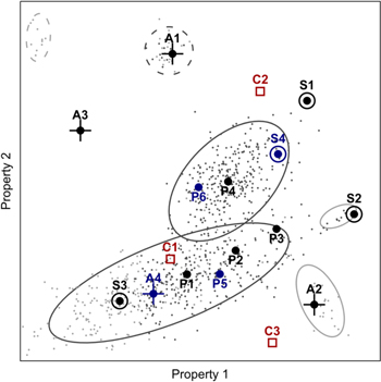
Figure 2. Hypothetical illustration of parameter space for a population of objects, showing the relations between different subpopulations (ellipses) and the Prototype (P), Superlative (S), and Anomaly (A) samples. Prototypes (plain dots) probe the "cores" or bulk of the subpopulations, Superlatives (ringed dots) probe their "rims" (as observed), Anomalies (crossed dots) include the seeming outliers. Observational selection effects give us a biased sample of the objects, where unobserved objects (light gray points) may be concentrated in some regions and observed objects (dark gray points) in others. While some subpopulations may be recognized (dark, solid outlines), others may be unrecognized because too few examples are known (light outlines) or they are too extreme to be linked with the other objects (dashed outlines). In addition, some objects in the Exotica Catalog may be selected by other criteria than those plotted (blue). A small Control (C) sample (open squares) includes "objects" that turned out to be unreal or mundane upon examination; they may have originally been thought of as prototypes, superlatives, or anomalies.
Download figure:
Standard image High-resolution imageIn all cases, our understanding of the diversity of targets will be filtered through selection biases, observational capabilities, and our theoretical categories. A subpopulation itself may span a wide range of characteristics, and thus no single target may represent its entire subclass. In those cases, we may artificially divide the span into several "bins" and choose representative examples from each bin (as in P1, P2, and P3 in Figure 2), as we do with the stellar main sequence, despite forming a continuum. This also allows us to impose some constraints when the new phenomenon occurs for a restricted parameter space region within the subpopulation. Objects may have extreme properties because they genuinely are superlative among the actual population, in turn because they are simply at the tail of a distribution (S1) or they actually are part of an unrecognized new subclass ; (S2), or just because we cannot detect the many more extreme objects (S3). Even "false" or apparent superlatives are useful in expanding the range of explored parameter space, as if we added extra "bins" to a sequence, because interesting phenomena may be biased in the population even while being common. Finally, anomalous outlier objects may be examples of an observed group whose sources are not yet identified (A1), the first example of an otherwise unobserved subpopulation (A2), or be genuinely unique (A3). As theory and observations advance, these outliers may be explained and added to the inventory of subpopulations. All these different possibilities are interesting for at least one of the motivations for the Exotica Catalog, although which motivation depends on why an object is a Prototype, Superlative, or Anomaly. Adding to the complexity is the number of possible dimensions of parameter space, so that some objects may be selected by criteria not evident in any one visualization (P5, P6, S4, and A4).
Thus, to address the core motivations (Section 2.2), the Exotica Catalog has four parts:
- 1.A Prototype sample including one of each type of astrophysical phenomenon (Motivations I and IV). We emphasize the inclusion of many types of energetic and extreme objects like neutron stars (Motivations II and III), but many quiescent examples are included too.
- 2.A Superlative sample that includes objects of known types that are on the tail ends of the observed distribution of some properties to better span the range of objects in the universe (Motivations I, II, and IV).
- 3.An Anomaly sample that includes inexplicable sources noted in the literature (Motivations II, III, and IV). A subsample includes previously published ETI candidates (Motivations I, II, and III).
- 4.Finally, a Control sample that includes "sources" that are unphysical, like the zenith, or objects that have been revealed to be mundane or nonexistent. These nonexistent sources may have originally been proposed as typical, extreme, or outlier objects (Figure 2). These targets will help us get a better handle on systematics (Motivation V).
In addition, we plan on doing occasional pointings at random positions on the sky. That will ensure we do not miss any completely unknown phenomenon because we are looking at known objects, allowing a nonbiased sample of the sky (Motivation I). Postbiological ETIs living in interstellar space are a possible example of a hostless phenomenon.
Despite the Prototype/Superlative/Anomaly division, the Exotica Catalog results in only a very coarse sampling of relevant parameter spaces. It is possible that conditions for the evolution of ETIs (or other interesting phenomena) are very stringent, and they will only be found in a very small subset of the space (see speculation that ETIs evolve only around "solar twins"; Fracassini et al. 1988). Even if the "window" is in the core of the parameter space clouds, the Exotica Catalog could easily miss them. This is a fundamental issue with its low-count approach. A high-count survey is needed to constrain these possibilities by covering parameter space with a fine grid and selecting objects from each bin. This grid approach was applied to the stellar color–magnitude diagram (CMD) in I17, although the grid was limited in extent, resulting in more extreme stellar objects being excluded. 21
4. The Prototype Sample: A Treasury Survey
The Prototype Sample is the largest portion of the full Exotica Catalog. The objects and source classes are listed in Table A1 in Appendix A.
4.1. Classification of Objects
The Prototypes form the bulk of the Exotica Catalog and represent our effort to have "one of everything." The range of things we would like includes both long-lived objects and localized phenomena. To build this catalog, we need some classification system to enumerate the different kinds of things. We start with a high-level classification system with 13 main categories listed in Table 1. These categories have extremely different evolutionary mechanisms and power sources, and they might each have a chapter in an undergraduate textbook or have an entire advanced textbook to themselves. Nonetheless, they are narrower than the three "kingdoms" proposed by Dick (2013). In analogy with the "kingdoms," we call these categories phyla, emphasizing both the shared fundamental traits and the vast diversity within them, and allowing for higher-level "root" categories. 22
Table 1. Phyla of Astronomical Phenomena: A High-level Classification System Used in the Exotica Catalog
| K64 Rating | Phylum | Characteristics | Example |
|---|---|---|---|

| Minor bodies | Solid, small, typically irregular shape, modification mostly from cratering after initial 26Al differentiation | 1I/'Oumuamua |
| I | Solid planetoids | Hydrostatic equilibrium; solid, possibly with liquid oceans; round; geology plays key role in interior evolution; thin atmosphere with insignificant mass compared to body | Titan |
| I | Giant planets | Hydrostatic equilibrium; fluids dominate mass and evolution; larger than Earth; typically high internal heat luminosity; formation by gas accretion onto solid core | Jupiter |
| II | Stars | Hydrostatic equilibrium; plasma; powered by nuclear fusion or sometimes gravitational contraction; no solid cores; includes brown dwarfs and protostars by convention | Sun |
| II | Collapsed stars | Supported by degeneracy pressure if at all; luminosity primarily from release of stored thermal, rotational, or magnetic energy | Sirius B |
| II | Interacting binary stars | Evolution of component stars affected by mass transfer; substantial luminosity from accretion, surface nuclear burning, or shocked outflow; often compact object is mass recipient | SS 433 |
II 
| Stellar groups | Gravitationally bound collections of stars, which do not otherwise interact for the most part; little to no dark matter | 47 Tuc |
II 
| Nebulae and ISM | Diffuse gases and plasmas; includes flows of matter to/from stars and diffuse galaxy; generally not self-bound | Orion GMC |
| III | Galaxies | Gravitationally bound, dominated by dark matter; generally contain vast numbers of stars, gas, and possibly a central black hole; gravitationally bound | M81 |
| III | Active galactic nuclei | Powered by accretion onto a supermassive black hole; includes gas flows on and off SMBH, frequently with jets and particle-filled bubbles | Cygnus A |
| III | Galaxy associations | Dark matter dominates internal gravitation; gravitationally bound collections of galaxies and intracluster medium | Virgo Cluster |
III 
| Large-scale structures | Unbound or loosely bound structures on ≫Mpc scales; includes high-order arrangements of galaxies and diffuse gas (IGM); non-virialized | Shapley Supercluster |
| Any | Technology | Structures built intentionally, frequently for processing of matter, energy, and information; so far only known to exist on/near Earth | Voyager 1 |
| ⋯ | Reference | Sky locations only important relative to observer | Solar antipoint |
Note. The "phyla" are used to group objects in the Prototype and Superlative samples by shared physical traits. From a SETI perspective, they indicate the need for very different techniques necessary for astroengineering, as reflected in the amount of used power measured by the Kardashev (1964) scale rating of on left.
Download table as: ASCIITypeset image
ETIs would probably need distinct engineering methods to harness members of different phyla. They span the Kardashev (1964, hereafter K64) scale, which groups technological ETIs broadly by the amount of power they consume. On the K64 scale, Type I ETIs harness the amount of power available on a planet, Type II ETIs harness the power available from a Sun, and Type III ETIs harness the power available from a galaxy, with proposed extensions to allow for levels beyond the range I–III and fractional levels. The power usage increases by a factor of order 10 billion between each K64 level. Table 1 gives a very rough estimation of the K64 rating available in each phylum.
There are edge cases like brown dwarfs that might fit in several categories, which we have placed according to convention or our judgment. To the natural categories we have added technology. Human artifacts in space are part of the optical and radio sky and are thus part of the astrophysical landscape now (e.g., Maley 1987; Combrinck et al. 1994; Tingay et al. 2013a; Corbett et al. 2020; Hainaut & Williams 2020; note the inclusion of artificial satellites in Gott et al. 2005). Our primary aim in SETI is to find (or rule out) other examples of this category. We have also added a category for reference points not corresponding to any physical points. Transients are also discussed separately (Section 4.4).
The phyla, while covering the breadth of astrophysics, are too coarse to form an exhaustive Prototype list by themselves. Obviously, hugely different possibilities for habitability and exploitation exist for an asymptotic giant branch (AGB) star and a red dwarf, for example, or a white dwarf and a black hole. Thus, we have broken down these categories into much more fine-grained types for the Prototype catalog. Some formal classification schemes already exist in the literature, most notably Harwit (1981) and Dick (2013). There are also three classification systems designed as metadata for organizing the literature that nonetheless have played a huge role in astronomical research: the old AAS journal keyword list, 23 Simbad's object classification system (described in Wenger et al. 2000), and most recently the Unified Astronomy Thesaurus (Frey & Accomazzi 2018). 24
We found none exactly fit our needs, usually being too coarse-grained in most respects (e.g., not emphasizing the great differences between interacting and detached binary stars) or too detailed for a subset of phenomena (e.g., the many narrow types of dwarf novae). Nevertheless, these systems did serve to ensure coverage of the gamut of astronomical objects. To supplement these classification systems, we consulted review articles and textbooks, which frequently describe classification systems used for particular types of astrophysical phenomena, and how they are distinguished. Discovery papers announcing new classes of phenomena also are useful for assembling a list of classes. Trimble's Astrophysics in 1991–2006 series (starting with Trimble 1992 and ending with Trimble et al. 2007) provided general overviews of the entire field for those years and highlighted newly discovered phenomena.
Astrophysical phenomena can be classified according to a wide range of characteristics. An object's composition, evolution, environment, and kinematics could all affect their attractiveness as a habitat for ETIs, or indicate new phenomena at work. One example is the asteroids, which may be classified according to orbit or composition. We therefore included several overlapping classification systems. Some Prototypes do double duty, acting as representative examples of several of these overlapping classes, to help keep the number of objects manageable.
Some classes of objects are excluded, usually because they are too impractical to observe. These included diffuse "objects" like the interstellar medium as a whole and very large structures like the Fermi Bubbles (Su et al. 2010). In addition, we required classes to have at least one example that was fairly well established to serve as the Prototype. For example, carbon planets, open cluster remnants, and dark matter minihalos are omitted because there have been no confirmed examples.
Although our goal is to have "one of everything" for the Prototype catalog, our focus is not entirely even. We cannot be entirely consistent about how fine-grained each category is, as it relies on subjective judgments about how to distinguish types. We have included finer subclasses when they may be relevant to SETI. Among these are the noninteracting double-degenerate binary stars, which have been proposed as possible "gravitational engines" (Dyson 1963). We also included some subclasses because their members have unusual properties that might indicate or motivate ETI presence. Hypervelocity stars, for example, might be good places for ETIs interested in extragalactic travel to settle. A couple of large classes that lie on a continuum of properties, namely main-sequence stars and disk galaxies, have been broken up to ensure good coverage over the possible range of environments they can host.
To complete a broad census of the cosmos, we also consider the possibility that habitability changes with cosmic time (see Loeb et al. 2016). Luminous AGNs, explosive transients, and galaxies with immense star formation rates (SFRs) and chaotic morphology were more prevalent at high redshift (e.g., Elmegreen et al. 2005; Madau & Dickinson 2014), with unknown effects on the evolution of ETIs and their technological capabilities (for additional speculation on some of these effects, see Annis 1999a; Ćirković & Vukotić 2008; Gowanlock 2016; Lingam et al. 2019). We partly mitigate the sensitivity losses over the vast luminosity distances by selecting gravitationally lensed galaxies. Our EIRP sensitivity will thus be boosted by about an order of magnitude for the selected objects. There is also the potential for gravitational microlensing from foreground objects, which has been known to magnify individual z ≳ 1 stars by over a thousand (Kelly et al. 2018), allowing us to achieve better EIRP limits for small high-z populations.
4.2. Prototype Selection
Each class's Prototype is selected to be a fairly typical example, even if the object type itself is unusual. The reason each object is chosen as the Prototype is given in the extensive notes to the catalog available online. When available, we generally pick objects that are well-studied and explicitly called a "prototype," "archetype," "benchmark," or something similar, like the "prototypical" starburst M82 (e.g., Seaquist & Odegard 1991; Leroy et al. 2015). This will provide us with the greatest context if we discover something. However, because Breakthrough Listen has unique capabilities, these observations will not be redundant with previous studies.
Although not directly referred to as such, stars have prototypes in the form of spectral standard stars, which we have used when practical. Classes of variable stars (including interacting binaries, like cataclysmic variables) are named after well-known examples, and we generally adopt the eponymous object as the Prototype. In two cases, we substituted another object if it is much closer and well studied: TW Hydrae for T Tauri stars (Zuckerman & Song 2004), and AG Car for S Dor–type Luminous Blue Variables (Groh et al. 2009).
A principle we adopted, especially when explicit prototypes are lacking, is to use objects with high citation counts, which we take as a proxy for how well studied an object is. We adopted this criterion by either selecting nearby objects filtered by object type in Simbad, or by viewing the objects in a prominent catalog for a type in Simbad (Wenger et al. 2000). Then we sorted by number of citations and examined a few objects with the highest citation count. We are mindful that well-cited objects may be particularly well studied because they host a rarer phenomenon or are anomalous rather than representative. 25
A final consideration is that we pick objects that are easy to observe and set meaningful limits on. Nearby objects are generally preferred. Not only are they usually well-studied and well known, but in a survey with limited integration time, we set tighter limits on novel signals from nearby objects. We also try to pick Prototypes that have already been observed by Breakthrough Listen as part of its nearby stars and nearby galaxy programs, or other campaigns. Because these have been selected by distance, already-observed objects also tend to be nearby and frequently have high citation rates anyway.
4.3. The Role of the Prototype Sample Compared to Previous Standards
We expect that a list of "prototypes" as in the Exotica Catalog will be useful to the general astronomical community. Although no single object can provide much information on the characteristics of a population (which requires a high-count study), single objects can be studied in greater detail with high-depth studies. The literature on a single prototypical object can therefore provide insight into the core traits of a phenomenon. Having prototypes is also useful for theorists, who generally want some sense about whether some new predicted effect is detectable or not. Often the best chance for discriminating theories is found by deep observations of nearby, bright, well-studied objects. 26
The primary literature already contains standard systems and explicit prototypes for types of objects, and the Prototype sample may seem redundant for these. Indeed, if one is interested in a narrower survey on only, say, asteroids, stars, or local galaxies of various morphologies, these are preferable.
Nonetheless, we believe the Prototype sample serves several useful purposes. First, even when we use these primary standards, the sample has collected them in one place for easier reference. This is important for a broad survey, of course—standards for stars and galaxies generally do not refer to each other—but may also be useful for a narrower survey, as there can be overlapping systems of classification based on different criteria (e.g., asteroid spectral types versus orbital classes). Second, as classification systems evolve, even a "standard" object may be listed under contradictory types, and it may not be clear which to use (for example, differing galaxy morphology types in de Vaucouleurs et al. 1991 and Buta et al. 2015). We have done our best to choose targets whose classifications are stable. Third, and most important, many of the object types listed in the sample do not have formalized classification systems with explicit standards. References to the consensus prototypes may be scattered far and wide among hundreds of papers, and it is useful to compile these objects in one place. Some types, particularly those discovered by large surveys or at high redshift, may be studied only in bulk with no individual object standing out. This can lead to an "embarrassment of riches" where the literature provides useful population studies but no guidance on choosing an example of the phenomenon. 27 For added utility, we are hosting online notes on the catalog. 28 These describe our reasons for selecting a particular object as a Prototype, potential caveats for the selection, provide citations to works where they are given as prototypes or standards, and in some cases give alternates that may be better suited for observation.
4.4. The Challenge of Transients
Among the panoply of celestial phenomena, transients pose special challenges for any attempt to observe "one of everything." Of course, everything in astronomy is transient on some scale: the planets, stars, galaxies, and black holes will all disperse over the next 10200 yr (Adams & Laughlin 1997); life, intelligence, and technology too all are expected to perish in a ΛCDM universe (Krauss & Starkman 2000). "Transients" here has an observer-relative definition, referring to objects that evolve in some way, typically brightness, on a timescale comparable to or shorter than the observing program. The importance of transients to our understanding of the cosmos has been recognized in the past few decades, and the past few years have seen a huge growth in detection capabilities and characterization, from radio (e.g., with the SETI-oriented Allen Telescope Array: Croft et al. 2011; Siemion et al. 2012; see also Murphy et al. (2017); CHIME/FRB Collaboration et al. (2018) for other recent examples) to optical (e.g., Law et al. 2015; Chambers et al. 2016), X-rays (e.g., Matsuoka et al. 2009; Krimm et al. 2013), gamma-rays (e.g., Abdo et al. 2016; Abdalla et al. 2019), neutrinos (e.g., Adrián-Martínez et al. 2016; Aartsen et al. 2017), and gravitational waves (e.g., Abbott et al. 2019a, 2019b).
Classes of transient events already number in the dozens, with a variety listed in Table A2. They span all of the electromagnetic spectrum and all messengers, all timescales from nanoseconds to decades and longer, and occur among most of the phyla, including some more properly considered Anomalies (Section 6). Although some are mundane visual effects, like eclipses, others contribute profoundly to cosmic evolution, like the r-process element birth sites in supernovae and neutron star mergers. We excluded in Table A2 those phenomena that induce only small variability (e.g., planetary transits), or are continuously ongoing rather than episodic (e.g., variable stars).
If there were no constraints on observations, we would like to observe at least one of each of the transient classes in Table A2. This follows from a broad-minded perspective on the possible forms of ETIs. Both known and hypothetical transients have been studied as possible technosignatures. More speculatively, conceivably some ETIs live on a completely different timescale than humans: perhaps whole societies of rapidly evolving artificial intelligences or neutron star life rise and fall in moments (see Forward 1980). Practical considerations make observing every known transient class in the table impossible. The most important reason for the difficulty is that we have to be pointing the telescope at the right point on the sky when the transient occurs. In order to detect a member of a rare transient class, we would either have to commit our facilities to staring and waiting for an event, or use facilities that observe much of the sky. Future wide-field instruments could be helpful (Section 9). Although there is no such facility in radio above 1 GHz or optical associated with Breakthrough Listen, we have pilot programs with the low-frequency facilities LOFAR (Low-Frequency Array; van Haarlem et al. 2013) and MWA (Murchinson Widefield Array; Tingay et al. 2013b) with wide-field capabilities.
Some transients repeat. These are listed in the first two sections of the Table. The hosts of repeating transients in Table A2 represent object types in their own right listed in the Exotica Catalog. A few transients occur at predictable times because their timing is the result of orbital motion: these include the periodic comets and OJ 287's flares. We may schedule observations during examples of predicted transients, as resources permit. Most are unpredictable, though, so simply knowing where they happen is of little help in ensuring a transient is observed. We would need to rely on alerts, and observations of the event itself will be dependent on our access to the facilities.
Other transients occur only once, at least on human timescales, as listed in the second section of Table A2. With these, we not only are unable to schedule observations of a transient example, we generally cannot study the pretransient progenitor. 29 Any hope of observing them requires an alert and a flexible observing schedule. While we may learn of an ongoing transient event through Astronomer's Telegrams (Rutledge 1998) 30 and Gamma-ray Coordinates Network (GCN) circulars, 31 we cannot guarantee that we will be able to slot in observations in time. Furthermore, some transients are so short lived—minutes or less—that they would be over by the time we received any alert. If the event occurs in the field of view of a radio telescope with a ring buffer, a trigger or prompt alert can allow us to beamform on it using temporarily stored voltages in the buffer (e.g., Wilkinson et al. 2004). Otherwise, we can only hope to observe the after effects of these short-lived transients. It is also possible short-lived transients are technosignatures of a larger ETI society that is still observable after the event itself is over. Hence, we include anomalous transients as objects in their own right in the Anomaly sample (Section 6).
Finally, a few transients are common enough that they invariably will occur during our observations, as listed in the final part of the table. Because these are generally not coming from the sources we are interested in observing, they in fact have the opposite problem of most transients: they are a form of interference that we cannot avoid even though we want to.
5. The Superlative Sample
The Superlative sample expands the reach of the Exotica Catalog survey across a wider range of parameter space (Section 3). These are objects that are among the most extreme in at least one major physical property, the record breakers. Perhaps ETIs, or unusual natural phenomena, are biased to very atypical examples of space objects, like the hottest planets, the lowest-mass stars, or the richest galaxy clusters. Extreme physical properties can also be a sign of different evolutionary histories or even new subtypes of phenomena. For example, pulsars with very short rotation periods are the result of a mass transfer phase during their evolution (Alpar et al. 1982). Table B1 in Appendix B lists the members of the Superlative sample, and the ways they are superlative.
5.1. Classification and Superlatives
Classification is an important factor in determining whether an object is really a superlative at the tail end of its class's properties, the prototype of a new class, or even a unique anomaly. In astronomy, some kinds of objects fall on a continuum in terms of properties, but are conventionally delineated by an arbitrarily chosen range. An example is the spectral type of a star: there is a continuous range of temperature, but the boundaries of the spectral types themselves do not directly map onto different evolutionary trajectories or habitability. Objects at the boundary of these classes have no special significance. We thus focus on the superlatives of easily distinguishable classes. Thus, we give superlatives for the phyla (Section 4.1), which is our coarsest level of classification. We include superlatives for some intermediate level classes, particularly within the solar system and by distinguishing white dwarfs, neutron stars, and black holes. Yet even the use of phyla does not completely solve the problem of overlapping categories. The smallest subbrown dwarfs have the same mass as the biggest giant planets (as is the case for the coldest member of the star phylum listed); galaxies overlap with stellar associations, with globular clusters forming a continuum with ultracompact dwarf galaxies.
An object may have properties that are so outstanding that we consider it an Anomaly. The basic distinction we make is that a Superlative should still be clearly a member of its class, governed by the same physical processes. Superlatives are drawn for the tail of a class's distribution, while Anomalies can appear to lie far outside it, inexplicably so.
5.2. Properties Considered: Superlative in What Way?
An object can stand out in one of many possible quantities. In principle, there are hundreds: the abundance of every element, absolute magnitude in every possible filter band or frequency, quantities describing internal structure, and velocities in different frames are all possibilities.
Additionally, we could take advantage of known empirical relations between quantities and include outliers from these relations as "superlative." These superlatives with respect to relations can actually indicate new object classes: objects lying far off the stellar main sequence are the giants and white dwarfs, both fundamentally different from dwarf stars, for example.
There are a great many such relations, however. The observable and physical properties of objects generally fall into "clouds" surrounding manifolds describing these relations in high-dimensional parameter space (Section 3; Djorgovski et al. 2013). If we wish to include the entire "rim" of each cloud, the "superlatives" would include all of the objects forming the boundary of that cloud, lying the farthest away from the manifold. Indeed, searching for such outliers is one proposed method to search for new phenomena (Djorgovski et al. 2001). The number of possible combinations of variables is vast, each corresponding to one small piece of the boundary, and we conceivably could include them all. It is impractical to select and observe all such objects.
We avoid proliferation by focusing on a small number of quantities that describe the basic properties of objects, which usually apply to most to all of the phyla. We consider the basic characteristics to be size, quantified by radius, mass, and number of members; composition, quantified by density and metallicity; and energetics, quantified by bolometric luminosity and temperature. When appropriate, mainly for objects with well-characterized orbits like planets, we include kinematics or position, quantified by space velocity and orbital semimajor axis and/or period. Finally, we include era, in the form of ages for planets and stars, and redshift for larger or brighter objects like galaxies. Some additional properties are included for certain object classes when they fundamentally regulate an object's behavior and are easy to find in the literature. For planets, we also consider some basic characteristics of the host star (mass, luminosity, surface temperature, and metallicity). Magnetic fields and rotation periods are included for neutron stars. An organizational parameter (number of levels in a system's hierarchy) is also included for multiple stars.
5.3. Finding Superlatives in the Literature
We used several methods to try to find Superlative objects. Starting a search for a Superlative involves reading through literature (generally as part of the Prototype and Anomaly search) and being alert for mentions of record-breaking objects. Sometimes the search started outside the peer-reviewed literature. Wikipedia maintains several lists of Superlative objects; 32 although we do not consider its entries as final, the objects it lists are generally among the most extreme, providing a place to start, and it includes links to relevant papers. Sorting major catalogs on VizieR 33 (Ochsenbein et al. 2000) or exoplanet.eu 34 (Schneider et al. 2011)by key quantities also gave us candidates. When we find a paper describing a candidate Superlative, we look at citing papers in the Astrophysical Data System (ADS; Kurtz et al. 2000), as anything that supersedes the object is likely to cite the previous record holder. We also look for papers describing previous record holders, and the papers that cite those, especially if the Superlative's measurements are uncertain.
Ideally, we wish to use objects that are explicitly described as being superlative in some regard in the literature. These can be announced by papers in journals like Nature or Science. 35 In other cases, the record may not be heralded prominently as the subject of a paper, but we found it mentioned in a paper while searching for Prototypes or Anomalies: the most massive supercluster (Shapley), for example (Kocevski & Ebeling 2006, while researching the Great Attractor). Review papers or compendiums sometimes highlight objects that are outliers and can be useful in this regard. 36 Trimble's Astrophysics in 1991–2006 series contained sections explicitly highlighting extreme objects (even referring to them as "Superlatives" in Trimble 1992), although in practice we found many of them had either been included already or were superceded since publication. 37
Many cases are less certain. Papers sometimes proclaim the extraordinary nature of an object without explicitly stating it is superlative. One case is the Superlative R136 a1, which is noted to have an extraordinary mass ( ∼ 300 M⊙), the highest in recent literature, without being explicitly said to be the most massive known star (Crowther et al. 2010).
Sometimes it seems that no one keeps track of certain extremes, and measurements may not be all that reliable. While there are many cases of extremely low-metallicity stars or galaxies being touted (e.g., for Superlatives in our catalog, Caffau et al. 2011; Keller et al. 2014; Simon et al. 2015; Izotov et al. 2018), few papers describe very high-metallicity stars or galaxies (a few exceptions are Trevisan et al. 2011; Do et al. 2018), and none proclaim a single Superlative. As we do want to include a superlative high-metallicity star, we looked through several catalogs listing stellar metallicities: Cayrel de Strobel et al. (2001), Hypatia (Hinkel et al. 2014), Bensby et al. (2014), PASTEL (Soubiran et al. 2016), CATSUP (Hinkel et al. 2017), PTPS (Deka-Szymankiewicz et al. 2018), and Aguilera-Gómez et al. (2018). These often gave contradictory measurements; a star that is the highest metallicity in one is relatively normal in another. In this case, we looked for a star that was frequently among the highest metallicities and reliably supersolar metallicity, settling on 14 Her (Gonzalez et al. 1999 comments on its high-metallicity explicitly, supporting its selection). As our goal is to sample the range of astrophysical phenomena, we thus prefer reliable outliers over including the most extreme objects with unreliable measurements. Very large catalogs often include these extreme superlatives, but do not comment on them. For example, PASTEL contains dozens of stars listed with [Fe/H] > +1.0, although these results are not replicated in other catalogs. We disregard these cases as likely being due to model inadequacies or measurement errors.
Some superlatives are not included at all. This is particularly the case when one class blends into another and the superlative depends simply on where the boundary is set, with many objects lying upon the border consistent with measurement errors. The most massive planet and the least massive brown dwarf are excluded superlatives for this reason (see the extensive discussion of the issue of classification in Dick 2013). Other reasons include the case when the potential Superlatives are heavily disputed, or when the objects have not been localized enough to follow up on—both circumstances applying to the most massive stellar black holes, because of difficulties in modeling X-ray binaries and the lack of counterparts for gravitational wave events.
Of course, we cannot guarantee that the Superlatives listed here are literally the most record-breaking objects in the universe. New record breakers are being discovered all the time. We expect to update the list as these are discovered.
5.4. On "True" and "Apparent" Superlatives
An important caveat is that the diversity of known objects is limited by our observational capabilities (Section 3). Whole regions of parameter space are inaccessible, and thus some Superlative objects will change with time. This is particularly true when considering the smallest, least luminous, or farthest objects. Indeed, these currently unobservable objects may be both interesting to SETI and actually dominate the population: consider the case of old neutron stars, which are expected to be so numerous that one is within ∼10 pc (e.g., Ofek 2009), would have several properties interesting for astroengineering without the intense radiation environment, and any example of which would qualify as Superlative. If we are looking for objects that stand out because they are engineered (as in Motivation II), or testing the hypothesis that ETIs are attracted to the most extreme objects only, then apparent Superlatives based on observational selection effects are of little use. Nonetheless, as mentioned in Section 3, merely apparent Superlatives are useful in that they expand the range of parameter space sampled. Put another way, if observational selection effects are hiding many sources, then the average source that we know about—and thus its representative in the Prototype sample—are actually atypical and the listed Superlative lets us probe a more typical example. Apparent Superlatives allow us to search for new phenomena that are biased toward certain environments (Motivation I) but not requiring the most extreme conditions possible (ETIs who build structures around all neutron stars below a certain spindown luminosity, for example).
Still, because they favor different motivations and test different hypotheses, we indicate our estimation of whether a Superlative is likely to be truly extreme among the cosmic population or not with the "True?" column in Table B1. The "true" superlatives include those where we would expect to be able to detect an object that was much more extreme (e.g., the most massive galaxy cluster), or when there are good theoretical reasons to expect there are no objects that are much more extreme (e.g., the faintest hydrogen-burning star). In some cases, we expect the listed Superlative to be the most extreme within the solar system, Galaxy, or Local Group but are uncertain if more extreme examples exist too far away to probe; these are indicated by special symbols. In many cases, though, we are unsure whether the Superlative is "true" or not, and these are marked with a question mark.
6. The Anomaly Sample
Anomalies are phenomena with observable properties that do not easily fit into current theories, not even roughly. Upon discovery, they frequently spur theorists to develop many new hypotheses and explore new mechanisms that might operate in the universe (as happened with gamma-ray bursts and continues to happen with fast radio bursts; Nemiroff 1994; Platts et al. 2019). Wild early speculation about alien engineering also tends to be associated with Anomalies, although to-date natural explanations have been eventually found. Nonetheless, it has often been encouraged to examine Anomalies for evidence of ETIs and any distinct signs of alien intelligence will be an Anomaly upon discovery (Djorgovski 2000; Davies 2010). Examining these anomalies does not only have to reflect a belief that they are alien engineering. Anomalies may also induce natural phenomena that mimic ETIs and are interesting in that regard (Motivation III). By examining these anomalies, we get a better sense of what to expect from the non-ETI universe, and a better sense of what is not normal. Thus, the presence of an object in the Anomaly sample is not a statement of belief about artificiality; many of the objects are clearly natural if unusual, like Iapetus.
The targets in our Anomaly sample are listed in Tables C1 and C2 in Appendix C.
6.1. Types of Anomalies
We use a supplementary classification scheme for Anomalies that groups them by the nature of their anomalousness. 38 Our hope is that it will aid both further searches for anomalies in diverse data sets and inspire new ideas about technosignatures (for example, as Class I or V anomalies).
This system has six classes.
- 1.Class 0 objects are those that are not anomalous from an astrophysical point of view, although they can be exotic in terms of SETI. We define Class 0 anomalies as a likely member of a known, explained population even if the classification is ambiguous, with no evidence for unknown phenomena at work. Almost all of the Prototypes and Superlatives fall in Class 0. An object can still have ambiguous classification without actually being mysterious; Pluto in the early 2000s was Class 0. Alternatively, an object that is unidentified because it has multiple good explanations remains Class 0: IRAS 19312+1950 may be either a young star or an AGB, but seems readily explainable (Nakashima et al. 2011; Cordiner et al. 2016).
- 2.Class I anomalies are likely members of a known, explained population, with normal intrinsic properties, but located in an anomalous environment or context. In other words, the object itself is not mysterious, only where it is. This also includes objects with inexplicable kinematics. Hot Jupiters were Class I anomalies until it was understood that gas giants could migrate (Mayor & Queloz 1995; Guillot et al. 1996).
- 3.Class II anomalies are likely members of a known, explained class, but whose properties quantitatively fall far outside the usual distribution. Class II anomalies are qualitatively similar to other objects of the same type. Millisecond pulsars, for a short time after discovery, were Class II because of their extreme spin (Backer et al. 1982). Candidate megastructures identified by infrared emission in excess of the expected value (as identified by the far-infrared radio correlation of galaxies, for example; Garrett 2015; Zackrisson et al. 2015) or abnormally faint optical emission (Annis 1999b; Zackrisson et al. 2018) are examples in a SETI context.
- 4.Class III anomalies are likely members of a known, explained class, but displaying a qualitatively new and unexplained phenomenon. These phenomena generally are not even observed around most (or any other) members of the class. Saturn's rings are a classical example, as their nature as debris belts took centuries to understand despite Saturn clearly being a planet (Dick 2013). Candidate SETI signals found in targeted surveys of nearby stars through the traditional methods of ultranarrowband radio emission or nanosecond optical pulses would be Class III anomalies.
- 5.Class IV anomalies are members of an unexplained or unknown phenomenon class. They may be identified only in one wave band, without counterparts in any others. Current explanations generally have plausibility issues. Many of the famous discoveries of the past century were originally Class IV anomalies: among them, Galactic synchrotron emission (Jansky 1933), quasars (Schmidt 1963), pulsars (Hewish et al. 1968), gamma-ray bursts (Klebesadel et al. 1973; Nemiroff 1994), and now fast radio bursts (Lorimer et al. 2007; Platts et al. 2019). They are, however, relatively rare. Candidate SETI signals found in wide-field surveys are frequently Class IV, including the Wow! signal (Dixon 1985; Gray & Ellingsen 2002).
- 6.Class V anomalies are objects or phenomena that appear to defy known laws of physics, whether the object itself is identifiable or not. These are extremely rare. In very special cases they may herald an upheaval in our understanding, as the Galilean satellites and solar neutrino problem did, but usually they are simply in error (e.g., the notorious case of candidate superluminal neutrinos in an early version of Adam et al. 2012, which was a nonlocalized Class V anomaly).
These classes, all else being equal, roughly increase in order of mysteriousness. Judgments about the classification of an anomaly will vary with new data and different emphasis. For example, in the 18th century, was Saturn a planet with the anomalous feature of rings (Class III), or were the rings themselves an anomalous object (Class IV)? Other considerations are whether an Anomaly has some theoretical explanation, if a problematic one, and the confidence that the anomaly is real. We list those with partial explanations as Class 0/x in Table C1 (where x is in the range I–V). We avoid purported anomalies whose existence we judge have been rejected by the astronomical community.
6.2. Collecting Anomalies
The search for Anomalies in the literature is even more associative and subjective than finding Prototypes and Superlatives. While there is plenty of discussion of mysterious classes of objects like FRBs, to our knowledge, there has not been an attempt to create a list of anomalous objects. An Anomaly might consist of a single object or event that does not attract a lot of outside attention, especially if it is poorly characterized.
A few Anomalies are well known in the SETI literature, including KIC 8462852 (Abeysekara et al. 2016; Boyajian et al. 2016; Wright et al. 2016; Wright 2018a; Lipman et al. 2019) and 1I/'Oumuamua (Bialy & Loeb 2018; Enriquez et al. 2018; Tingay et al. 2018b; 'Oumuamua ISSI Team et al. 2019). The abundance pattern of Przbylski's star, particularly the possible presence of short-lived radioisotopes (Cowley et al. 2004; Bidelman 2005; Gopka et al. 2008), has been informally discussed online as a possible technosignature (see Whitmire & Wright 1980), which is how we learned of it. 39 Others were known to us through general knowledge (e.g., the CMB cold spot, Cruz et al. 2005). Still other anomalies were found using the help of the Astrophysical Data System, particularly while looking at citations and references to evaluate an object (ADS; Kurtz et al. 2000). Papers that identify Anomalies frequently cite previous (explained or unexplained) Anomalies. 40 Papers about Anomalies can cite well-known review articles or compendiums specifically so they can situate or differentiate their mysterious object from mundane phenomena. 41 As with Prototypes and Superlatives, we scanned Trimble's Astrophysics in 1991–2006 review series. 42 Wikipedia also has a "list of stars that dim oddly" 43 that includes several of the Anomalies, although we generally found them by using other sources and not all stars listed there are anomalous.
The process was mainly serendipitous, however. We did search ADS for terms like "anomalous," "mysterious," "enigmatic," and "unusual," although they tended to mostly turn up papers that were about relatively normal objects. 44 Those papers were mainly about minor puzzles that we do not consider inexplicable enough to rise to Anomaly status, although this is a subjective judgment. We also had to ignore object classes with "anomalous" in the name, such as Anomalous X-ray Pulsars (now identified as magnetars). Similar searches on the Astronomer's Telegram archives netted several examples. 45 Papers about recently identified mysterious objects appear in arXiv 46 or journals like Nature and Science, where they garner attention. 47
Transients are frequently unexplained upon discovery, and they are well represented in the sample. Even though the events themselves are over, anomalous transients may hypothetically be technosignatures of K64 Type II–III ETIs. We may then hypothesize there to be other technosignatures—and other Anomalies—coming from these societies, which would share the same field as the transients themselves did. As a very speculative example, perhaps the large early-type galaxy M86 is one such location, as it hosts two Anomalous X-ray transients. 48
Some anomalies in the literature are not localized objects or are otherwise impractical to observe. These are listed in Table C3 for readers interested in a more complete understanding of currently inexplicable phenomena.
For this present catalog, we had to search for Anomalies through a literature scan. There is great interest in searching for anomalous signals in instrumental data with machine learning, however (e.g., Baron & Poznanski 2017; Solarz et al. 2017; Giles & Walkowicz 2019). In the coming years, these automated efforts will likely flag new objects with unusual properties that can be added to future versions of the Exotica Catalog (Zhang et al. 2019).
6.3. Previous SETI Candidates
A special subset of Anomalies, one especially relevant for Breakthrough Listen, is that identified by other SETI programs. Signals identifiable as technosignatures essentially have to be anomalies, otherwise they could always be given a more mundane explanation and it would not be effective as a SETI search. Indeed, Earth, or the solar system, would appear to be a Class III anomaly to radio astronomers with sensitive-enough telescopes, due to its unnatural narrowband radio emission.
Candidate signals identified by other SETI searches are included in the subcatalog listed in Table C2. These include suggestions of narrowband radio emission (Dixon 1985; Blair et al. 1992; Horowitz & Sagan 1993; Colomb et al. 1995; Bowyer et al. 2016; Pinchuk et al. 2019), nanosecond-duration optical pulses (Howard et al. 2004), optical spectral features consistent with picosecond-cadence pulses (Borra & Trottier 2016), infrared excesses compatible with waste heat from megastructures (Carrigan 2009; Garrett 2015; Griffith et al. 2015; Lacki 2016b), and one example of an apparently vanished star (Villarroel et al. 2016). Most of the non-SETI Anomalies are not single-instance transients, and therefore their anomalous natures can be confirmed by independent groups. The SETI candidates have a more uncertain existence, though, and may have been mundane (e.g., RFI).
Despite not widely being considered strong evidence of actual ETIs, we include them because they match previous specific predictions about technosignatures. In addition, Breakthrough Listen has followed up on claimed SETI candidates in the past, to date verifying none (Enriquez et al. 2018; Isaacson et al. 2019). Finally, the wide variety of technosignatures covered helps ameliorate the difficulty of learning about anomalies with unfamiliar techniques or subfields. When a great many candidate ETIs are given, we include only a few examples, chosen according to the brightness of the stellar host (Borra & Trottier 2016), the evaluated quality of the candidate (Howard et al. 2004; Carrigan 2009; Griffith et al. 2015; Zackrisson et al. 2015), or the signal-to-noise ratio of the event (Horowitz & Sagan 1993; Colomb et al. 1995; Bowyer et al. 2016).
7. The Control Sample
The final group of targets is those we observe with the expectation of not observing anything new. Instead, they provide a baseline set of observations for comparison with any positive detection of a new phenomenon, a control sample for the SETI experiment. If some subtle systematic or source of interference is generating false positives, it should eventually show up during observations of appropriately chosen control sources. We could thus rule out the false positive by comparison with the results of the Control sample.
7.1. The Control Sample
The first part of the Control sample is along the lines of the other samples, a list of astrophysical targets (Table D1 in Appendix D). These are targets that were once thought to represent a new or anomalous phenomenon but that turned out to have very mundane explanations. We can simulate our response to transients or the discovery of an anomaly by looking at purported transients that turned out to be banal.
As an example, Bailes et al. (1991) reported the first discovered pulsar planet around PSR B1829–10. If Breakthrough Listen had been operating in 1991, we surely would have scheduled a rapid campaign to observe PSR B1829–10, similar to our campaigns observing 1I/'Oumuamua and FRB 121102, because it was among the first exoplanets reported in the literature. A year later, however, the same authors traced the pulsar timing signal to an error in the treatment of Earth's orbit (Lyne & Bailes 1992). We would have acquired deep radio observations of a planet that turned out not to exist. Any detection would likely have been the result of an error in our analysis or perhaps have come from the pulsar itself.
Because of limited data and the difficulties of interpretation, there have been many mistaken claims in astronomy. We chose the objects and phenomena in Table D1 on a few principles. First, there should be consensus that the claimed discovery was in fact in error, preferably by the original authors themselves. Second, most of the claimed discoveries should have appeared to be confident enough to have provided a strong impetus for observations. The majority appeared in the peer-reviewed literature, although KIC 5520878 and GW 100916 were explained in the same paper that reported them (Hippke et al. 2015). The exceptions are GRB 090709A, for which a claimed 8 s quasiperiodicity was reported in several GCNs by multiple groups (Golenetskii et al. 2009; Gotz et al. 2009; Markwardt et al. 2009; Ohno et al. 2009) before being dismissed (see Cenko et al. 2010; de Luca et al. 2010); HIP 114176, a false star in the Hipparcos catalog; and Swift Trigger 954840, which could likewise have prompted observations but was not in fact an astronomical event. 49 Third, we avoided picking bright or exceptional sources, where we might expect new phenomena, in favor of nonexistent or anonymous targets. An example of a source we excluded is the X-ray binary Cygnus X-3, which was widely considered to be a brilliant TeV–EeV gamma-ray and cosmic-ray source in the 1980s before the early detections lost credibility (Chardin & Gerbier 1989; see also Archambault et al. 2013 and references therein for recent gamma-ray observations). Similarly, we excluded Barnard's Star, a nearby star that had two candidate exoplanets in the 1960s–1970s (van de Kamp 1963; Choi et al. 2013), because it actually does have a planet, albeit one much smaller, listed as a Prototype (Ribas et al. 2018). Fourth, sky coordinates needed to be reported, which prevented us from including perytons, seeming atmospheric radio transients later explained as RFI from a microwave oven (Petroff et al. 2015).
Our inclusion of a target in the Control sample is not meant to disparage the claimants. Science has a long history of observational errors, some of which have prompted deeper studies that in turn revealed real phenomena. The mistaken discovery of planets around PSR B1829–10 encouraged the announcement of the actual first pulsar planets around PSR B1257+12 (Wolszczan & Frail 1992; Wolszczan 2012). The retraction then encouraged careful scrutiny of PSR B1257+12's planets, building a more solid case for their existence. The apparent discovery also prompted theoretical work into the origins of pulsar planets. Another early exoplanet announcement was HD 114762 B, an apparent warm super-Jupiter detected by the radial velocity method (Latham et al. 1989). In a case of terrible luck, this real object has in recent years been shown to be a red dwarf orbiting HD 114762 in a nearly face-on orbit (Kiefer 2019). 50 Yet it turns out there really are warm and hot gas giants, including those much bigger than Jupiter, and they really could be detected through the radial velocity method, in defiance of the expectations of the time (Latham 2012; Cenadelli & Bernagozzi 2015). Discoveries like these can open conceptual spaces, unexplored possibilities that were simply not thought of before. In other cases, a purported anomaly can be studied well enough that it becomes the prototype of an object class. This seems to be happening with NGC 1277, a prototypical red nugget galaxy studied because of the now-disputed extreme mass of its central black hole (Trujillo et al. 2014).
7.2. Could We Just Look at "Empty" Regions of the Sky?
Even with the Control sample, there is a danger that we could observe something real. HD 117043 probably does not have potassium flares (Wing et al. 1967), but for all we know it does have a planet with ETIs; it is even one of the I17 sample stars. Likewise, PSR B1829-10 is a real radio pulsar, even if it does not host planets (Lyne & Bailes 1992). Most of these are relatively distant, so only a very bright ETI signal would be discovered, but it remains a possibility. Of the Control sample, only about half correspond to actual astronomical objects (the others being GW 100916, Hertzsprung's Object, HIP 114176, OT 060420, the Perseus Flasher, Swift Trigger 954840, and VLA J172059.9+385226.6).
A more stringent set of Control sources would be to look at empty places on the celestial sphere with no objects at all. This is often not actually possible, though. A famous example is the Hubble Deep Field, chosen to be away from any known bright sources, which has thousands of galaxies (Williams et al. 1996). The beam size of the GBT at 1 GHz is about  , which would cover thousands of galaxies and trillions of extragalactic planets, and only one would need to send a bright broadcast in our direction.
At high frequency, radio beam sizes are smaller. It could be possible to slip a beam between known all stars and galaxies near 100 GHz with GBT, or 10 GHz with one kilometer baselines using MeerKAT. Even this would not guarantee the nonexistence of ETIs within the main beam. Red dwarfs, brown dwarfs, and white dwarfs would generally not be detectable from many kiloparsecs away and might exist in the beam, although hard limits on their abundance on sight lines toward the Magellanic Clouds have been set with microlensing surveys (e.g., Tisserand et al. 2007). But for all we know, some ETIs actually exist in the depths of interstellar space, away from all stars (Ćirković & Bradbury 2006). Perhaps they broadcast from starships (e.g., Messerschmitt 2015) or ride along ubiquitous interstellar objects like 'Oumuamua. Thus, there is no place on the sky that can be guaranteed to be free of ETIs. The main utility of looking at "empty" sky regions as a control is to limit the prevalence of relatively faint signals from nearby, known objects.
7.3. Unphysical Targets
The ultimate Control source is one that cannot possibly be an actual source at all. Then if we do observe what looks like an ETI signal, we can be quite sure it is some systematic issue, whether instrumental or caused by interference. An unreal source can be simulated by selecting an unphysical trajectory for where the telescope is pointed, and then treating the output data as if it came from a single location on the sky. Sources outside of the solar system near the celestial equator are bound to rise in the east and set on the west like all other noncircumpolar sidereal sources; to do otherwise would be to violate causality. Even within the solar system, the motion of objects is constrained.
As an example, consider the zenith as a "source." It is a very special point from the viewpoint of the observer, convenient and easily attention grabbing. But practically speaking, the zenith actually sweeps out a band on the sky. No distant source beyond one light-day could remain at the zenith because of causality. Unless the observatory is on the equator, no object in Earth orbit would remain at the zenith. Any such beacon would have to be both nearby and would require expensive, power-intensive maneuvers. Furthermore, the zenith's sightline depends on the specific location of the observatory, an improbable coincidence unless the makers mapped Earth thoroughly, recognized radio telescopes, and somehow determined which ones were doing SETI. If needed, other possible unreal sources abound by choosing other implausible tracking trajectories: we could track faux "targets" that rise in the west and set in the east, that rise in the north and set in the south or vice versa, that move along circles of constant sky altitude as if we were at a pole, or jitter randomly on the sky.
The GBT and Parkes are able to stare at fixed altitude-azimuth positions to conduct drift scan surveys of the sky. It is also possible to do raster scan surveys where the telescope is tracked along "impossible" paths to map the sky quickly. The key difference is that we would analyze the data not as a scan moving across the sky, but as if the telescope's celestial coordinates were fixed: we would look for signals that persist for the entire "observation" instead of rising and falling as the beam sweeps over them. We must also be aware that signals might spill in from the sidelobes of the beam.
We will not usually have control over where the dishes of MeerKAT are pointed. Nonetheless, we do have the power to electronically beamform within the primary field of view. We could move one commensal beam to a new random location in the field every millisecond, making jumps that are about a degree long in an instant. No celestial source could follow such a trajectory.
The use of "fake sources" is closely related to our extant techniques to constrain RFI in our radio observations. Bright RFI from elsewhere in the sky can impinge on the detector through the dish's sidelobes. During observations, we employ an ABABAB (or ABACAD) strategy: we spend five minutes pointed at a target and then move to look at a different target for five minutes. We alternate between on- and off-target five-minute pointings for a total of three each. Signals that are detected through the sidelobes will appear in both the ON and OFF pointings, whereas a genuine signal that is not exceedingly bright will disappear in the OFF pointings (Enriquez et al. 2017; Price et al. 2020). The advantage of using scans as "sources" compared to ON/OFF strategies is that we will be able to constrain systematic issues that persist for only a few seconds. A somewhat related strategy is possible on Parkes, where the multibeam receiver points at seven sky locations simultaneously. Interference coming in from the sidelobes will appear in several beams at once. 51
Analyzing the faux sources will require some updating of our metadata and software. In addition, the unphysicality of the simulated "sources" depend on their movement on the sky, which only is significant if the signals are prolonged. Thus, they are no better than the Control sample or random sky locations in looking for false positives in pulse searches. Other facilities interested in using the Exotica Catalog may not even have the capability to do raster scans. For these reasons, we maintain the Control sample as an easy to implement check for systematics.
7.4. Technological Sources: Looking for Trouble
A final set of objects that could act as a check is the technology Prototypes (listed at the end of Table A1). Technology, particularly RFI, is the biggest source of false positives in SETI. Our observations of the technology Prototypes should build a small library of RFI for comparison with potential ETI candidates. Indeed, we already have serendipitous observations at the GBT that could contribute to such a library, including from GPS and Iridium satellites. Unlike the other Controls, when we look where we expect to see no signals, with these Prototypes, we are looking where we do expect to see a signal, one that confounds our other observations, to better understand our systematics.
Not all technological RFI can be studied in this manner, though. Aircraft and ground transmitters would not be covered by these observations. Nonetheless, satellites remain one of the biggest contaminants, and are likely to become much worse with the launch of Internet satellite constellations.
8. Discussion of the Full Exotica Catalog
8.1. Target Demographics
The full Exotica Catalog contains over 900 entries and more than 800 distinct targets (Tables E1 and E2 in Appendix E). It is about 40% of the size of the I17 nearby stars and galaxies catalog, and thus observing all objects would represent a significant effort on our part. The targets are distributed across both hemispheres on the sky, with concentrations in Cygnus and the Kepler field within it, the Galactic Center and the inner Galactic Plane, the Large Magellanic Cloud, and around the Virgo (and Coma) Cluster (Figure 3). The breakdown of the different catalogs into samples, into phyla, and objects we have already observed is given in Table 2.

Figure 3. Map of objects in the Exotica Catalog in equatorial coordinates. Each phylum is given its own symbol, with Prototypes in black and Superlatives in blue. Anomalies are plotted in red and Control sources in gold. The plane of the Milky Way is shown as the gray curve.
Download figure:
Standard image High-resolution imageTable 2. Exotica Catalog Summary
| Property | Prototypes | Superlatives | Anomalies | Control | Total | |
|---|---|---|---|---|---|---|
| Non-SETI | SETI | |||||
| Entries | 598 | 187 | 125 | 36 | 17 | 963 |
| Distinct | 536 | 155 | 115 | 33 | 17 | 816 |
| ...Minor body | 79 | 13 | 6 | 0 | 0 | 93 |
| ...Solid planetoid | 29 | 22 | 2 | 2 | 0 | 39 |
| ...Giant planet | 21 | 12 | 2 | 0 | 0 | 33 |
| ...Star | 120 | 15 | 34 | 13 | 5 | 178 |
| ...Collapsed star | 35 | 24 | 8 | 0 | 2 | 64 |
| ...Interacting binary star | 47 | 3 | 1 | 0 | 0 | 50 |
| ...Stellar group | 29 | 18 | 9 | 1 | 1 | 54 |
| ...ISM | 42 | 6 | 1 | 0 | 0 | 48 |
| ...Galaxy | 81 | 23 | 3 | 10 | 0 | 116 |
| ...AGN | 33 | 13 | 9 | 0 | 0 | 55 |
| ...Galaxy association | 14 | 9 | 0 | 0 | 1 | 23 |
| ...LSS | 3 | 1 | 1 | 0 | 0 | 5 |
| ...Technology | 15 | 0 | 0 | 0 | 0 | 15 |
| ...Unknown | 0 | 0 | 42 | 9 | 0 | 50 |
| ...Not real | 4 | 0 | 0 | 0 | 8 | 12 |
| Solar system | 103 | 26 | 5 | 0 | 0 | 118 |
| Sidereal | 433 | 129 | 110 | 33 | 17 | 698 |
| I17 stars | 49 | 2 | 2 | 1 | 2 | 55 |
| I17 galaxies | 15 | 0 | 1 | 0 | 0 | 16 |
| Other BL observed | 2 | 0 | 3 | 0 | 0 | 4 |
| New targets | 470 | 153 | 109 | 32 | 15 | 741 |
Note. Entries that are cross-listed in two different phyla are counted in the number of distinct targets in each phylum.
Download table as: ASCIITypeset image
Over 160 (∼20%) distinct targets are in what Dick (2013) calls the Kingdom of the Planets: the minor bodies, the solid planetoids, and the giant planets. Two of the most important properties of these bodies—mass and stellar insolation—are plotted in Figure 4. The giant planets span over a factor of 100,000 in insolation (∼20 in temperature for a constant albedo), and the solid planets span nearly as large of a range. The giant planets cover a full range of masses from super-Jovian to Neptunian and insolations from ≳1000 Earth to 0.001 Earth (and GJ 3483 B at ∼ 10−10 Earth insolation). The solid planetoids we have chosen cover the range of temperate to hot temperatures and sub-Earths to super-Earths, with a tail of low-mass cold planetoids from the dwarf planets and large moons in the solar system. Minor bodies, almost all from the solar system, cover temperate to cold environments and a factor of over 10 billion in mass.

Figure 4. Diagram of planetary mass and stellar insolation for planets in the Exotica Catalog. Solar system bodies are marked in deep blue, those around stellar remnants in sky blue, and those around protostars in gold. Minor bodies (including planets hosting ring systems) are denoted by triangles, solid planetoids by circles, and giant planets by squares. Bodies in the Superlative sample are marked by a ring around them, and those in the Anomaly sample are marked by an overlaid cross.
Download figure:
Standard image High-resolution imageThe Exotica Catalog will allow us to conduct a thorough initial reconnaissance of the solar system. All of the major planets, 52 all IAU-recognized dwarf planets, and most of the larger moons 53 are included. But an even greater coverage of the solar system comes from the inclusion of the minor bodies, which form the third-largest phylum in the Exotica Catalog (∼11%). There are a great many minor-body Prototypes, which comes from the use of fine types. This is partly because minor bodies form a large population that can be well studied in the solar system, but we include them also to ensure we examine objects from every region of the solar system. The importance for SETI is the possibility of ETI probes in the solar system, which may have gone unnoticed (Papagiannis 1978; Freitas 1985; Gertz 2016; Benford 2019; see also Wright 2018b; Schmidt & Frank 2019 for more extreme possibilities). Their radio presence will begin to be constrained with Exotica Catalog observations.
The phylum most represented in the final catalog is stars, with almost 180 distinct targets (∼22%). This is partly driven by the fine classifications we use in the Prototypes catalog, particularly with the main sequence divided into narrow spectral subtypes. The fact that we have already observed most of the main-sequence Prototypes allow us this luxury, because we will not need to repeat most of those observations (Enriquez et al. 2017; Price et al. 2020). Yet the stars also include a number of types not at all represented in I17. We see this in Figure 5, the CMD and Hertzsprung–Russell (HR) diagram of stars in the Exotica Catalog. The Exotica Catalog expands the coverage of Breakthrough Listen to include supergiants and hypergiants at the top of the diagram, a region of parameter space entirely missed by the I17 sample. O dwarfs are finally covered as well. Sprinkled around the diagram are some unusual stellar types that result from binary evolution, which swell the ranks of stars in the Prototypes sample. Among them are the hot subdwarfs (sdB and sdO), which sit in between the white dwarfs and hot main sequence on the left of Figure 5. The Exotica Catalog also includes some star types that are unusual in ways other than where they sit on the HR diagram, like variable and hypervelocity stars. Not shown in the CMD are brown dwarfs, mostly invisible in optical light, which supplement the ones observed in Price et al. (2020).

Figure 5. Color–magnitude (left) and HR (right) diagram of stars (circles) and white dwarfs (sky blue squares) in the Exotica Catalog. Protostars and pre-MS stars are colored gold, brown dwarfs are dark orange, and post-interaction stars are dark violet. The hosts of exoplanets are also included as open circles (stars) or open squares (white dwarfs). Stars in I17 are shown as gray dots. Superlatives and Anomalies sources are marked as in Figure 4.
Download figure:
Standard image High-resolution imageCollapsed stars and interacting binary stars are smaller phyla, each with about 50 to 60 objects (∼8% and 6%, respectively). Collapsed stars have a moderate representation in the Prototypes sample—they broadly fall into white dwarfs (with both mass and spectral categories), neutron stars, and the hard-to-observe black holes—but the compact objects power a rich variety of interacting binary stars. There are also about two-thirds as many Superlative collapsed stars as Prototypical ones, especially because the well-studied pulsars allow for precise studies of their properties. The Exotica Catalog includes five symbiotic systems (excluding symbiotic X-ray binaries), twelve cataclysmic variables and related white-dwarf-powered binaries, and over 20 X-ray binaries. These objects have been practically ignored in SETI, but they are among the most powerful and dynamic objects in the universe. Including them allows us to start probing the idea that they draw energy-hungry ETIs (as in Lacki 2020). These extreme objects are also good bets to look for other new astrophysical phenomena. A few more collapsed stars in detached binaries reside among the stellar associations.
Stellar groups and the ISM are also smaller phyla (∼7% and 6%). Even within the Galaxy, the simple open/globular cluster divide is supplemented by division of the globular cluster into distinct populations and the inclusion of Superlative clusters. Observations of other galaxies have revealed star clusters different from those in the Galaxy, and have identified a number of Superlative clusters with densities and masses far more extreme than anything nearby. To these are added detached stellar multiples and unbound stellar associations. The ISM includes a panoply of clouds in different phases and on different scales. Because of its diffuse nature, though, some of its most important features cannot be divided into discrete targets or are not practical to observe, particularly large structures of hot gas like the Local Bubble (Snowden et al. 1990). A variety of energetic phenomena drive a similar variety of expanding bubbles. We note the inclusion of cosmic-ray ISM features, particularly the Cygnus Cocoon (Ackermann et al. 2011).
Galaxies form the second-largest phylum (∼14%). Even though we use a relatively coarse division along the Hubble (1926) "tuning fork," they are supplemented by a rich variety of subtle morphological features (Buta et al. 2015) and peculiar galaxies (see Arp 1966). In fact, about one-fifth of the galaxy prototypes simply cover disk galaxy morphologies, such as lenses and rings. Just as some abnormal stellar types are the result of binary interactions, we have peculiar galaxy types from their own interactions. High-redshift galaxies only increase the panoply, as do the technosignature candidates identified by previous SETI studies.
Figure 6 summarizes their gross properties, mass and color. Included galaxies span a factor of ∼ 1010 in stellar mass. In terms of gross properties, I17 samples much of the same parameter space, and in fact includes many more faint red (dwarf spheroidal) galaxies. Note however that we were unable to find data to plot certain extreme dwarf galaxies like Segue 1, which are far smaller than the ones in I17. We also are excited by the outliers in the CMD, particularly IC 1101 (red circled dot at the far right), the Leoncino dwarf (black cross-dot at the lower left), and NGC 4650A (isolated black dot at the lower right). More profound differences are visible in the mass–SFR diagram, where highly star-forming galaxies stand out with respect to the I17 sample, particularly those at high redshift (open circles) and dwarf starbursts (purple dots at the center left), as does Coma P (circled blue dot in the lower left) and the Leoncino dwarf. These are entirely new regions of parameter space to SETI.
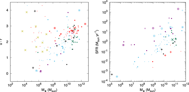
Figure 6. Mass–color (left) and mass–SFR (right) diagram of galaxies in the Exotica Catalog for which we could find or derive data. Galaxies classified as quiescent are shown in red, Green Valley galaxies in dark teal, main-sequence galaxies in sky blue, and starbursts in dark violet. Samples are marked as in Figure 4. Galaxies in other categories are classified according to morphological type, with the remainders in black. We also show I17 galaxies as small dots, and the Milky Way as the big teal ×. For the mass–color diagram, we include star clusters as gold asterisks, but exclude galaxies with z ≥ 0.1 due to k-correction effects. High-redshift galaxies are included in the mass–SFR diagram: those with z < 0.5 are marked with filled dots, and those with z ≥ 0.5 are marked with open circles.
Download figure:
Standard image High-resolution image
AGNs (∼7%) and galaxy associations (∼3%) are among the smaller phyla. We might have gone with finer AGN classifications, with Padovani et al. (2017) noting several dozen types posited over the years, but as per Padovani et al. (2017), we did not wish to cloud the Prototypes list with a menagerie of mostly overlapping types. On the other hand, galaxy associations have a richer (if still small) representation than might have been expected. A galaxy cluster, being virialized, can support some intriguing phenomena in its intracluster medium. Superlative galaxy associations almost match the number of Prototypes and include several rich galaxy clusters, which are unexplored in SETI.
The smallest phylum is large-scale structure (<1%). Its variety is limited because it has only begun to form. Furthermore, superclusters, walls, and voids have poorly defined boundaries and cover vast areas on the sky, and are excluded similarly to much of the ISM and IGM. We do include the Great Attractor, formerly a striking anomaly, in the form of the Laniakea basin of attraction (Tully et al. 2014). Also included is the superlative Shapley Supercluster, the densest and richest region in the local universe. This supercluster is a massive collection of rich galaxy clusters and has bound a region over 10 Mpc in radius; its gravitational pull actually entirely subsumes the flow from the Great Attractor (Kocevski & Ebeling 2006; Chon et al. 2015; Hoffman et al. 2017). It is an exceptional place for aspiring Kardashev Type IV ETIs, and it will evolve into one of the most outstanding "island universes" as the accelerating cosmic evolution cuts off long-distance travel over the next trillion years (Heyl 2005).
Finally, about 70 (∼9%) targets stand apart from the conventional astrophysical phenomena. About two-thirds of them (∼6% of the catalog) are unidentified, consisting of both SETI-related and non-SETI related Anomalies. Another fifth, in the unique phylum of technology, consists of our own technosignatures, which we may someday extend with non-Earthly examples. Nine spurious and miscellaneous targets complete the Catalog.
Further discussion of specific issues in classification are in the Appendices A (Prototype), B (Superlative), C (Anomaly), and D (Control). More extensive notes on the entries in the catalog and their selection will be available online. 54
We note that the entries in the catalog are not all independent entities. Some are collective objects that contain other entries in the catalog or are "siblings" in the same cluster. In addition, some "new" objects in the Exotica Catalog are related to objects in the I17 catalog. Examples include the several objects located in the Virgo Cluster, which itself is a Prototype. In these cases, one observation may actually cover several objects, and they can be treated as all one object. Table E3 lists these relationships.
8.2. Catalog Presentation
The objects in the catalog are listed in Table E1 (targets within the solar system) and Table E2 (sidereal targets outside the solar system). Each distinct source has been assigned a unique identifier that is simply an integer in the range 001–816, with increasing values for objects that first appear in the Prototype, Superlative, non-SETI Anomaly, SETI Anomaly, and Control samples. These tables also include basic data about the sources, with references discussed in Appendix E.1.
In addition, we will host an online database on the Exotica Catalog sources. The database will include detailed notes motivating our selection of a particular object, links to the object on Simbad or other databases, and references for the object and its type.
8.3. The Exotica Catalog and Inhomogeneous Observations
In many ways, the Exotica Catalog is driven by theory, which both provides the motivation and guides the classification systems used to select Prototypes and Superlatives and evaluate Anomalies, and is intended for instruments, as a kind of "treasury survey" they may do. As a high-breadth catalog, the Exotica Catalog represents an extremely diverse range of targets. In general, the possible observations that can be done on themselves vary from object to object. One clear case of this is the great difference between our knowledge of solar system and sidereal objects. Our space probes can journey to solar system objects and even land on some, providing "ground truth" that is as yet not possible with objects outside the solar system. Whereas an exoplanet is generally understood in terms of its bulk properties (aside from those with temperature maps), solar system bodies can be mapped with individual geographic regions and even individual landing sites studied. Direct comparison can therefore be problematic. Even in SETI, there are qualitatively distinct technosignatures that can be sought in the solar system, namely abandoned artifacts on planetary surfaces (Davies 2012; Davies & Wagner 2013).
The observations will be relatively homogeneous for the instruments that Breakthrough Listen is currently using, however. The biggest distinction among objects is whether they are resolved or not. This distinction already exists in the I17 catalog, where some galaxies are resolved while other galaxies and all stars are not. As with resolved galaxies in the I17 catalog, we expect we will observe a single pointing of the resolved objects and then add more pointings, resource permitting. All included solar system objects except for the Sun and Moon are unresolved even with the GBT for ν ≲ 10 GHz, and many to much high frequencies. In all cases the data products will be the same for the radio instruments, a collection of spectral products, and possibly some voltages, as was the case for our observations of 1I/'Oumuamua. Of course, the sensitivity we will achieve for the objects in the Catalog will diverge by orders of magnitude, but this would be true even if we were observing low- and high-z galaxies, for example. We expect the same is true of other individual instruments that might observe the Exotica Catalog, including radio telescopes, to some extent X-ray telescopes (although planets will generally be resolved; see Bhardwaj et al. 2007), and gamma-ray and neutrino detectors (e.g., Abdo et al. 2011a; Aartsen et al. 2021).
These considerations do result in the exclusion of one object that we would have included as a Prototype and an Anomaly (Table C3): Earth itself. Our ground-based radio instruments are only able to sample small regions of Earth's radio environment. We have no way of measuring Earth's integrated radio emission, much less its optical technosignatures, except through the indirect method of moonbounce experiments (McKinley et al. 2013; DeMarines et al. 2019).
9. All-sky and Random Surveys
The least biased strategy of when and where to look is to look everywhere all the time, with an all-sky survey. Even if ETIs inhabit objects we have not even detected yet, we would still be able to see their activities. Similarly, we would be able to look for natural objects that are completely unanticipated in our current paradigms (Wilkinson 2016). Because the sky has already been mapped across the spectrum, such unanticipated sources either are intermittent, very faint, or are unrecognized in current data sets.
The need for all-sky all-the-time surveys has been recognized in SETI and other fields of astronomy. Ideally, we would be able to keep the data permanently from such sources. This would both allow us to do searches for precursors when an anomalous event is triggered or to find anomalies years later in reanalyses. At present, no radio SETI facility exists with all these capabilities, despite the strong possibility that any "beacons" have a very low duty cycle to conserve energy. In the future, dipole arrays may be constructed to fulfill this purpose (Garrett et al. 2017). In the optical and the near-infrared, the Pano-SETI experiment aims to monitor several steradians instantaneously for short pulses (Cosens et al. 2018). Outside of SETI, there are multiple instruments with wide-field, high-cadence capabilities in the optical (Law et al. 2015), X-rays (Krimm et al. 2013), gamma-rays (Atwood et al. 2009; Abeysekara et al. 2017a), neutrinos (Aartsen et al. 2017), and gravitational waves (Abbott et al. 2019a).
Wide-field facilities allow us to set meaningful constraints on unanticipated events at present. Very wide-field capabilities are already granted by LOFAR and MWA (e.g., Tingay et al. 2016, 2018a) and have been used for serendipitous constraints (Tingay et al. 2018b). MeerKAT, an array of 64 dishes of aperture 13.5 m, will allow us to synthesize dozens of commensal beams within the relatively large primary field of view. It will be possible to devote one beam to painting the entire primary dish field over and over, a miniature wide-field survey that is open to finding truly unknown sources at unknown locations. The Breakthrough Listen backend will also perform incoherent summing of the dish voltages during observations. Despite having less sensitivity (Sν larger by a factor of 8), the entire primary dish beam is covered, an instantaneous field thousands of times larger than a single synthesized beam. The incoherent summing will be our first steps toward all-sky surveys, which have the maximal breadth allowed. Because it needs to observe the extended Cerenkov light of air showers produced by gamma-rays, VERITAS always has a relatively wide field of view (Weekes et al. 2002). However, neither telescope's pointings are uniformly distributed across the sky.
A more limited unbiased search that is possible even on narrow field-of-view telescopes is to point at random targets on the sky. Some completely random positions on the celestial sphere can be added as a supplement to the Exotica Catalog; they may be observed like any other target or with long integration times as a "pencil beam" survey to achieve sensitivity to faint flux levels or very intermittent sources. This will also be possible with MeerKAT, which will perform long targeted observations of some sky regions during its nominal science operations. We could devote synthesized beams to a random point in the dish field to do a pencil beam survey with every observation.
The final possibility—that anomalies already are present in extant data sets—calls for keeping data until such time as innovative analyses can find them. There has been plenty of precedent for this scenario: the long-term variability of Boyajian's Star was recovered in Kepler data (Montet & Simon 2016); the Lorimer burst, the first reported FRB, happened in 2001 but was not reported until Lorimer et al. (2007); the first ANITA upwards neutrino shower was not reported for 3 yr after its detection (Gorham et al. 2018). Breakthrough Listen is devoted to making its data publicly available in accessible formats (Lebofsky et al. 2019). Moreover, on the analysis side, we are pursuing research in using machine learning to classify signals and look for anomalies (e.g., Zhang et al. 2019). These have the potential of evading our biases.
10. Exotica Efforts and Breakthrough Listen
As noted in Section 2.3, Breakthrough Listen's exotica efforts will include both observations of the targets in the Catalog and a flexible series of campaigns. In this section, we briefly discuss our engagement with exotica with both approaches.
10.1. Strategy for Observing the Exotica Catalog
The full Exotica Catalog includes over 800 distinct sources, over 40% of the number of targets in the I17 list. Priority is given to the I17 targets, however, with the Exotica Catalog nominally getting ≲10% of telescope time. This is especially a problem because many of the sources are extended. An additional constraint is disk space, which prohibits keeping the raw voltages from radio observations of the entire catalog. We present some strategies for dealing with these issues, which may be useful to other programs aiming to observe the Exotica Catalog.
The core of our strategy is to develop a prioritization system for the targets. With GBT, Parkes, and APF, we are free to select targets without the constraints of commensal observing. Furthermore, the GBT has a number of frequency bands to observe in, and we can choose which ones to emphasize. Thus, we do not need to carry out the full suite of observations we perform on the I17 stars and galaxies, and conversely we can spend more time on high-priority targets. Table 3 breaks down the radio data products for one possible prioritization plan, as might be implemented on the GBT. If all objects are observed with this plan, the Exotica Catalog would take ∼800 hr to observe and would generate ∼2.0 PB of data (∼1.6 PB of filterbank files). For comparison, the ∼1700 stars in the I17 catalog observed in all bands would take ∼8000 hr and would generate 14 PB of data. The amount of time spent at each rank is 150–350 hr. Restricting our Exotica Catalog efforts to the low- and mid-frequency bands observed in Price et al. (2020) would roughly halve the observing time, mostly spent on low-priority targets.
Table 3. Example Prioritization System
| Rank | Count | Total Data | Filterbank Products | Raw Voltages | Observed Bands | Extended Target Strategy |
|---|---|---|---|---|---|---|
| Maximal | 12 | ∼ 0.6 PB | 3 × 5 minutes ABACAD | 5 minutes in a low-, medium-, and high-ν bands for at least one pointing | All | ∼5 pointings, including core and axes |
| High | 30 | ∼ 0.4 PB | 3 × 5 minutes ABACAD | 1 minutes in medium-frequency band for one pointing | All (one pointing), three (other pointings) | ∼3 pointings |
| Medium | 60 | ∼ 0.3 PB | 3 × 5 minutes ABACAD | None | Three | ∼3 pointings |
| Low | ∼700 | ∼ 0.6 PB | As available | None | Single | 1 pointing |
Note. The ABACAD (and related ABABAB) strategies involve pointing the telescope on and then off target to constrain RFI; see Price et al. (2020) for further information. The data rates assume that half the objects at each rank are extended, for an order-of-magnitude estimate.
Download table as: ASCIITypeset image
As yet, prioritization is subjective. We intend to favor extreme phenomena: those with high luminosities and nonthermal emission across the spectrum. These are more likely to display new astrophysical phenomena. Higher luminosities also make them better suited for modulation as beacons by ETIs. Thus, we will include proportionally more pulsars, interacting binaries, and AGNs. We specifically will put maximum priority on the primary calibrators at radio frequencies and high energies: Cygnus A and the Crab Nebula, respectively (Kirsch et al. 2005; Perley & Butler 2017). The Crab Nebula specifically is known to flare (Abdo et al. 2011b; Tavani et al. 2011; Wilson-Hodge et al. 2011). Another thing we have in mind is to achieve the widest breadth in astrophysical environments and object type. We will assign high-to-maximal priority to at least one object of every phylum priority list. We also intend to prioritize Superlatives with extreme luminosities and several Anomalies.
The APF is capable of collecting high resolution spectra of exotica targets. Target acquisition is challenging for targets fainter than V ∼ 12 and those with large motions across the sky. As such, we expect to only be able to observe a limited subset of the catalog. Such a search for narrow wavelength signals would be different than that in Lipman et al. (2019) because the targets are producing almost no astrophysical optical signal.
Our time on MeerKAT and VERITAS is commensal; thus, we will be unable to choose where the telescopes are pointed or prioritize different targets. Some of the southern targets are likely to be primary-user targets of MeerKAT during its nominal observations. In these cases, we will be able to reuse the primary synthesized beam data for our observations. Others will likely enter the field of view during large sky area surveys. Additionally, Breakthrough Listen's backend will allow us to form dozens of commensal beams within the dish field of view. While most of these beams will be dedicated to the one million star effort of Breakthrough Listen, several will typically be available for exotica observing efforts. From time to time, we may substitute a suitable object in the MeerKAT field for a given Prototype by using supplementary catalogs. VERITAS has a wide field of view, with diameter of several degrees (Weekes et al. 2002). Many of the objects in the Exotica Catalog have been primary targets of VERITAS. Others are clustered near the targets, like M81 and NGC 3077 near M82 (VERITAS Collaboration et al. 2009), or the galaxies in the Virgo and Perseus Clusters (Acciari et al. 2008, 2009). Thus, for many of the northern Exotica Catalog targets, it will simply be a matter of collecting VERITAS's commensal observations and organizing them.
The large angular extent of many of the objects in the catalog pose another challenge, especially in high-frequency radio observations where the beams of the telescopes are very small. It would be impractical to map the full extent of the sources with the GBT and Parkes. For the low-priority sources, we will observe only the core or flux peak of the target, as a proxy for the potential for activity. There will be additional pointings for higher-priority sources, resource permitting, generally including two at the ends of the semimajor axis. In some cases where there are multiple well-defined interesting spots, we will target these (e.g., the hotspots of radio galaxies). Parkes' multibeam receiver will also be useful, because it covers seven times the sky area, although its frequency range is limited. The electronic beam-forming capabilities of MeerKAT will afford us more flexibility; we will be able to dedicate a synthesized beam to "painting" the entire primary field of view, allowing us to construct low sensitivity maps. The APF's nominal field of view of 1 arcsec2 will limit its use for extended exotica objects. VERITAS should be able to observe all but the largest targets in their entirety at any given moment.
Another part of our strategy will be to opportunistically take advantage of available time. As we complete observations of the I17 sample with our main radio facilities, the GBT and Parkes, more time will be freed up for exotica. Another tactic is to make use of the ON/OFF strategies we use to constrain RFI: we can use an exotica source as an OFF source during observations of a program star or vice versa, whereas previously we have used stars. The OFF observations themselves can be used for technosignature searches, using the ON observations to check for RFI (Price et al. 2020). Additionally, the remaining GBT observations are mostly at high frequency and are sensitive to the weather. When weather conditions preclude high-frequency observations, we can observe exotica sources at low frequency. A similar strategy may be employed at other facilities, perhaps taking advantage of time when the Moon is up for at least the brighter sources.
Finally, some of the targets in the Exotica Catalog have already been observed as part of previous studies. These will not need to be reobserved. This too could be adapted to other facilities, adapting the catalog to include sources that have already been covered.
10.2. Exotica Campaigns and Breakthrough Listen
Several focused programs to observe unusual classes of objects have been completed, and more are ongoing. These single- or few-target campaigns are complementary to both our primary high-count effort in observing stars and galaxies over a hundred nearby galaxies and also the high-breadth catalog. These have included:
- 1.Interstellar asteroids: A test case for SETI—The interstellar objects 1I/'Oumuamua ('Oumuamua ISSI Team et al. 2019) and 2I/Borisov (Guzik et al. 2020) were observed by us as they passed through the solar system. Starfaring ETIs might very slowly diffuse through the galaxy by hitching rides on comets. More pragmatically, our observing campaigns for 1I/'Oumuamua and 2I/Borisov act as rehearsals if a convincing ETI probe is detected. The 'Oumuamua observations included 2 hr each in the L, S, C, and X bands, allowing us to cover the entire rotation cycle of the object to an EIRP sensitivity of 0.08 W, comparable to some Bluetooth or WiFi transmitters (Enriquez et al. 2018). We also observe solar system asteroids that have been postulated to be captured interstellar objects, the first being the observation of (514107) 2015 BZ509 on Parkes for 10 minutes of total integration (Price et al. 2019b). These observations are being supplemented by observations of other candidate captured interstellar objects, effectively adding a new class of objects to the Breakthrough Listen program.
- 2.FRB 121102 and other FRBs: Transient astrophysics—The Breakthrough Listen backend can also be applied to phenomena thought to be natural. In Gajjar et al. (2018), we observed the repeating FRB 121102 with the backend on the GBT for an entire hour. On average, one burst was detected every 3 minutes, achieving the highest frequency detections of the anomalous object; we also independently confirmed the high rotation measure discovered by Michilli et al. (2018). The long time devoted to these observations allowed us to observe and characterize many bursts, which would not have been possible with a 5 minute observing time. This highlights the advantage of the flexible nature of campaigns, allowing us to achieve high depth. The backend of Parkes was able to record a real-time fast radio burst, FRB 180301, in commensal mode (Price et al. 2019a). Significantly, we were able to capture raw voltages on this anomalous object, greatly increasing the analysis possibilities. We expect to observe other FRBs in the future.
- 3.Ultracool dwarfs: Extending I17 —We have devoted time to specifically observe five nearby ultracool dwarfs of spectral types late M to early Y with Parkes, as reported by Price et al. (2020). The observations of each object was otherwise similar to those of the stars in the catalog. The purpose of these observations was to extend the completeness of I17, effectively supplementing it with a new object type. In the future, it might be possible to further increase the I17 catalog's breadth by running short campaigns on other object classes, such as nearby white dwarfs (see Gertz 2019).
- 4.SETI campaigns on stars: Following up on SETI candidates—Campaigns have also been undertaken on the facilities to test claims of technosignatures. Borra & Trottier (2016) reported the existence of a spectral comb in the Sloan spectra of dozens of Sun-like stars, which they interpreted as resulting from coherent pulses repeating on picosecond timescales. The two brightest of these stars were observed with the APF, but no signs of a spectral comb were found in the spectra (Isaacson et al. 2019). Other campaigns to follow up on individual objects that have been noted by SETI researchers include optical observations of Boyajian's Star with VERITAS (Lipman et al. 2019), radio observations of the Random Transiter (Brzycki et al. 2019), and radio follow-up of an ETI candidate signal from Ross 128 (Enriquez et al. 2019). These observations were scheduled rapidly, within four days for Ross 128. With campaigns, new high-priority targets can be followed-up rapidly, without waiting for the catalog to be updated.
These efforts demonstrate the uses of campaigns to supplement the Exotica Catalog: (1) rapid follow-up of new and time-sensitive discoveries, (2) deep observations of high-priority targets, (3) supplementing the primary program to expand its breadth, and (4) moderate count programs of unconventional targets. These advantages should apply to other programs as well.
11. Summary
Breakthrough Listen intends to spend ∼10% of its observing time on exotic objects. There are many reasons to search for technological intelligence in unconventional places. Unearthlike or nonbiological entities will not be constrained to live in Earthly habitats hospitable to lifeforms like us. It is also conceivable that some kinds of seemingly natural phenomena are the result of alien engineering. Yet there are good motivations for observing unusual objects even if ETIs cannot possibly live there. Extreme, energetic objects are more likely to produce unusual signals, particularly transients, that might be confused with artificial signals. Breakthrough Listen has unique instrumentation, and observation of a broad range of objects would benefit the general astronomy community. Finally, there could be unaccounted-for systematic errors in our systems that give false positives. Observing exotic objects and empty regions on the sky allows us to constrain these possibilities.
Whereas the nearby star and galaxy catalogs aim for depth and high count, efforts to look for exotica can be more broad, trying to peek at everything that might be interesting. Breakthrough Listen's approach to exotica is twofold. First, from time to time, we have dedicated programs that observe one to a few objects of one class. Although we sample only a few types of object this way, these types are very diverse. Efforts include observations of the interstellar minor body 'Oumuamua and the repeating fast radio burst FRB 121102. By focusing these efforts on just a few objects, we can achieve deep sensitivity with the long integration times devoted to them.
The other prong is the Exotica Catalog, which is the main focus of this paper. The Exotica Catalog aims to achieve the widest possible breadth, including the most diverse range of celestial phenomena possible. The catalog itself contains four samples:
- 1.The Prototype sample includes an archetypal object of each type of astrophysical phenomenon.
- 2.The Superlative sample lists record-breaking objects with the most extreme values of basic properties like mass.
- 3.The Anomaly sample contains objects and phenomena that are inexplicable by current theories, including candidate positive events from other SETI efforts.
- 4.A small Control sample includes objects once thought to be anomalous or noteworthy but that turned out to be banal or nonexistent and will be used as a check on systematics and to rehearse observations.
There are 816 objects in the total Exotica Catalog, which will be sorted into different levels of priority. About a dozen sources will be observed with maximum priority and will include raw voltage data in multiple bands. Most will be low priority and will be observed as allowed by time.
We hope that the Exotica Catalog will prove useful to other efforts, both within SETI and outside it, in characterizing the whole panoply of objects in the known universe.
Breakthrough Listen is managed by the Breakthrough Initiatives, sponsored by the Breakthrough Prize Foundation (https://breakthroughprize.org/).
This work would not have been possible without the extensive use of a number of online databases. It has made thorough use of the SIMBAD database, the VizieR catalog access tool, and the cross-match service XMatch, all operated at CDS, Strasbourg, France. We have also benefited immensely from the NASA Astrophysics Data System Bibliographic Services and the arXiv preprint server. This research has made use of the NASA/IPAC Extragalactic Database, which is funded by the National Aeronautics and Space Administration and operated by the California Institute of Technology.
We thank the referee for the comments, and we thank Jill Tarter and Ken Shen for suggestions and clarifications.
Appendix A: The Prototype Sample
A.1. Minor Bodies
We classify solar system minor bodies according to both orbital family and composition, with a small number of additional subtypes. Minor bodies of specific compositions might be selected by ETIs for mining (see Papagiannis 1978). From a SETI perspective, orbital families might be targeted by ETI probes to provide a unique vantage point over bodies like the Earth, or because they are dynamically stable for long periods of time and could accumulate a large number of artifacts (e.g., Benford 2019). There is a large overlap in some cases between spectral and orbital groups (as in DeMeo & Carry 2014), as with the E-belt and E-type asteroids, for which we use the same Prototype.
For asteroids, our spectral-type system is largely taken from Tholen (1984; see also Tedesco et al. 1989). We selected those types considered the most significant by Tholen (1984), adding those unique to one or a few members. Some intermediate classes that blend into larger "complexes" in the more recent Bus & Binzel (2002) taxonomy were omitted. In choosing the Prototypes, we were guided by the classifications of Tholen (1984), Tedesco et al. (1989), and Bus & Binzel (2002).
The comet orbital classifications were informed by Levison (1996).
"Distant minor bodies," adapting the "distant objects" term used by the Minor Planet Center, 55 refer to outer solar system bodies beyond the Jupiter Trojans that are not comets. The spectral-type system is that of Barucci et al. (2005) and Fulchignoni et al. (2008), with the latter guiding our Prototype selection. The division into orbital groups is based on the system in Gladman et al. (2008), which we consulted especially when selecting Scattered Disk and Detached objects. We aimed to select Prototypes that are almost certainly minor bodies and not dwarf planets, as indicated by a "probably not dwarf planet" designation on Mike Brown's website. 56
The small classification system for satellites into regular, irregular, and "collisional shards" in Burns (1986) informs our classification.
Hughes et al. (2018) informed our grouping of debris disks into cold, warm, and hot/exozodis.
A.2. Solid Planetoids
Planets were classed according to size and stellar insolation. Kepler result papers classifies planets by radius into Earths (<1.25 R⊕), Super-Earths (1.25–2 R⊕), Neptunes (2–6 R⊕), Jupiters (6–15 R⊕), and nonplanetary (>15 R⊕) (Borucki et al. 2011; Batalha et al. 2013). We adjusted this scheme by (1) setting the boundary between solid super-Earths and giant Neptunes at 1.5 R⊕, except when density is known (Rogers 2015; Fulton et al. 2017); (2) adding a sub-Earth category for radii < 0.75 R⊕ to cover planets like Mars where the habitability prospects are likely different (e.g., Wordsworth 2016); (3) using the Weiss & Marcy (2014) relation to translate the radii categories into mass categories when no radius is available, using the mean  of π/4 as a guide. The mass categories for solid planetoids are sub-Earths (≲0.4 M⊕), Earth (∼0.4–2 M⊕), and super-Earths ( ∼ 2–4.5 M⊕, unless densities are known).
We use the terms "hot," "warm," "temperate," and "cold" to group by insolation. Cold planets are outside the conventional habitable zone (roughly taken to be ≲0.25 Earth), temperate planets are within the conventional habitable zone ( ∼ 0.25–2 Earth), warm planets are interior to the habitable zone but with insolations ≲100 Earth, and hot planets have insolations ≳ 100 Earth. The distinction between "warm" and "hot" carries over from the giant planets, where warm planets around Sunlike stars are defined by period or semimajor axis (Dong et al. 2014; Huang et al. 2016; Petrovich & Tremaine 2016). The insolation range for "temperate" planets was chosen somewhat arbitrarily, partly to include Mars on the outside and leave no gaps with the "warm" planets as defined in the literature. Kopparapu et al. (2014) finds habitable zone boundaries that range from 0.8–1.4 Earth on the inside (generally near 1.0 au) to 0.2–0.4 Earth on the outside. All the "temperate" Prototypes have insolations of 0.39–1.1 Earth, a more conservative range, except for the temperate Jupiter HD 93083b with 1.8 Earth.
Dwarf planets in the solar system are classed according to the spectral type and orbit, similarly to minor bodies (Appendix A.1). With the exception of Sedna, only the IAU-recognized dwarf planets (Ceres, Pluto, Eris, Makemake, and Haumea) are listed as dwarf planets.
We added a "geological" classification intended to very roughly sample the diversity of surface environments and histories in the solar system, excluding Earth itself.
A.3. Giant Planets
Giant planets are classed according to insolation and size (see Appendix A.2). Where possible we use densities to distinguish between ice giants and gas giants. We also added a "Superjovian" category to cover a better range of planetary masses. In the literature, the minimum mass for "superjovians" has been defined as 1, 3, and 5 MJ (Johnson et al. 2009; Clanton & Gaudi 2014; Currie et al. 2014). We arbitrarily are guided by a threshold of ∼ 3 MJ and allow  values of 2–10 MJ.
An additional subcategory classifies giant planets according to (non-main-sequence) stellar host, with a final entry for a resonant chain system.
A.4. Stars
Our estimation is that the major distinction between different types of stars is based on evolutionary stage and stellar mass.
Low-mass protostars and pre-main-sequence stars are classed numerically in the literature as 0, I, II, and III according to obscuration, where II and III correspond to T Tauri stages (Lada 1987). We retain the distinction between class 0 and 1 protostars and T Tauri stars. High-mass protostars are given their own categories.
Subbrown dwarfs are too small to have fused deuterium but are believed to have formed similarly to stars, as opposed to giant planets (Caballero 2018).
Brown dwarfs and main-sequence (MS) stars are classed by Harvard spectral type. Each spectral type is divided into early (0–3), mid (4–6), and late (7+) subdivisions. Where possible we chose spectral standards as Prototypes (Morgan & Keenan 1973; Kirkpatrick et al. 1991; Walborn et al. 2002; Kirkpatrick 2005; Burgasser et al. 2006). We also favored stars in I17, because we have already observed a wide range of B through mid-M dwarfs. For brown dwarfs, we also tried to choose those with a mass that was clearly below the hydrogen-burning limit.
Covering post-main-sequence evolution is more complicated. Stars that are actually in distinct evolutionary stages can appear on the same place in the HR diagram, such as the red giant branch and the asymptotic giant branch. To start, we divided post-main-sequence stars into mass groups with qualitatively different evolution:
- 1.Very low-mass stars (initial mass ≲0.2 M⊙) are not predicted to have a red giant phase, but no isolated post-main-sequence examples are known (Laughlin et al.1997).
- 2.Low-mass stars (initial mass ∼ 0.2–2.2 M⊙) pass through a red giant branch (RGB) phase, terminating in a helium flash in their degenerate cores. The RGB star rapidly ( ≪ 106 yr) transitions to a core helium-burning (CHeB) phase before ascending the asymptotic giant branch (AGB). The ultimate remnant is a CO white dwarf.
- 3.
- 4.Transitional-mass stars 58 (initial mass ∼ 7–11 M⊙) proceed similarly to the intermediate-mass stars until the end of the AGB phase, whereupon they begin carbon burning as a super-AGB phase. Those with lower mass end as an ONeMg white dwarf, while larger ones may undergo electron-capture supernovae and possibly leave behind neutron stars (Karakas & Lattanzio 2014; Woosley & Heger 2015; Jones et al. 2016). The division between these two fates is not precisely known, so we do not make the distinction.
- 5.Massive stars (initial mass ∼ 11–40 M⊙) undergo later stages of core nuclear burning. They switch between being red and blue supergiants during these later stages (Gordon & Humphreys 2019). They may have pronounced mass loss that transforms them into Wolf–Rayet stars (Clark et al. 2012). Massive stars end with a core collapse, leaving behind a neutron star or black hole (Heger et al. 2003).
- 6.Very massive stars (initial mass ≳ 40 M⊙) leave the main sequence but are unable to become red supergiants, probably because of their extreme mass loss (Humphreys & Davidson 1979; Woosley et al. 2002). They instead become blue supergiants and blue hypergiants, and after the mass loss, Wolf–Rayet stars (Clark et al. 2012). The stellar remnant is a black hole or nothing at all (Heger et al. 2003).
ETIs living around stars in different groups would face different challenges when adapting to post-main-sequence evolution (for example, the post-helium flash contraction would require large-scale migration over just a few millennia to remain in the habitable zone). For low- and intermediate-mass stars, we preferred to use Gaia benchmark stars with well-determined masses (Heiter et al. 2015).
The evolutionary stages are supplemented with stars with atypical characteristics, including chemically peculiar stars, Be stars with decretion disks, pulsar-like stars, Population II stars, and a collection of pulsational variables. Peculiar stars that are the result of stellar mergers are emphasized because of their diverse and unique evolutionary histories (e.g., Jeffery 2008; Heber 2016).
A.5. Collapsed Stars
These are divided into white dwarfs, neutron stars, and black holes.
White dwarfs are mainly grouped according to mass (Liebert et al. 2005) or spectral type (Sion et al. 1983), with supplemental subtypes based on evolutionary, composition, magnetic, or variability characteristics.
Neutron stars are grouped primarily by their rotation rate and magnetic field. These parameters also control the emission we observe and are related to evolutionary state (e.g., Alpar et al. 1982; Olausen & Kaspi 2014).
Black holes are grouped by detection method. Only a few detached black holes are known with firm positions, and many candidates are disputed (e.g., Bodensteiner et al. 2020; El-Badry & Quataert 2020; van den Heuvel & Tauris 2020), constraining our choice of Prototypes.
A.6. Interacting Binary Stars
We group interacting binary stars powered by accretion by the nature of the mass donor and that of the recipient:
- 1.Semidetached and contact binaries—both components are stars (i.e., not stellar remnants).
- 2.Symbiotic stars—donor is a giant, recipient is a small early-type star or a white dwarf (Belczyński et al. 2000). Symbiotic systems including neutron stars are listed under X-ray binaries.
- 3.Cataclysmic variables (CVs)—donor is a late-type dwarf star, recipient is a white dwarf. They are further divided by variability/eruption characteristics (Osaki 1996; Schaefer 2010) and white dwarf magnetic field interaction with the accretion disk (Patterson 1994). Closely related are the AM CVn binaries, where the donor is a helium star or white dwarf, and the close binary supersoft sources where the donor is a higher mass subgiant (Kahabka & van den Heuvel 1997).
- 4.X-ray binaries—The recipient is a neutron star or black hole. They are further divided based on the mass of the donor (low mass or high mass) and still further by the mode of mass transfer and other characteristics (see especially Reig 2011; Kaaret et al. 2017). X-ray binaries with an extreme super-Eddington accretion rate or luminosity (including the ultraluminous X-ray sources) are given their own special subcategory. Two more empirical types where the recipient's nature is indeterminate round out the category.
In a few cases, stellar outflows rather than accretion dominates the system. These include systems where shocks dominate the luminosity (like colliding wind binaries), and the spider pulsars where a formerly accreting neutron star ablates its companion (e.g., Dubus 2013; Roberts 2013).
A.7. Stellar Groups
We include noninteracting binary and multiple stars with other stellar groups like star clusters. As in Eggleton & Tokovinin (2008), they are distinguished from clusters by their hierarchical organization. Binary systems are well represented in the I17 catalog, and we do not try to capture all combinations of stellar types or separations. We specifically include double-degenerate systems, however, which are not included in I17, and have the potential to be sites of ETI activity (Dyson 1963). A few binaries classified by how they are detected from Earth (heartbeat, eclipsing, self-lensing, chromospherically active) are included when they indicate distinct physical phenomena could be exploited for observation coordination by ETIs; visual, astrometric, photometric, and beaming binaries are excluded, however.
Globular clusters are classified according to the orbit classification of Mackey & van den Bergh (2005); additional subtypes are based on internal structure and luminosity. Other stellar clusters are divided into massive super star clusters, "faint fuzzies," nuclear clusters (including former nuclei of dwarf galaxies), and open star clusters.
Some unbound stellar associations are also included, when well-studied examples were not too large on the sky to be practically observed.
A.8. Interstellar Medium and Nebulae
The interstellar medium (ISM) as a whole has a complicated turbulent structure, although it is classically divided into hot, warm, and cool and cold phases (e.g., Cox 2005). Some structures in the interstellar medium are too large to practically study with our facilities: the hot ISM, the loops, the warm ionized medium, and so on. In terms of the general ISM, we focus on molecular clouds and H ii regions, which are relatively compact. These are classed according to column density into translucent and dark clouds, with the dark clouds further divided by scale. Molecular clouds have self-similar structure, and although they are sometimes labeled as complexes, clouds, clumps, and cores in the literature, the divisions are arbitrary (see Wu et al. 2010). H ii regions formed within the molecular clouds are also included and likewise grouped by density/size (Habing & Israel 1979).
Most of the entries in this phylum are structures produced by outflows from central engines and their interaction with the general ISM. These are grouped according to the nature of the central engine.
Additionally, we include a bubble of cosmic rays to represent the nonthermal ISM, and two circumgalactic medium clouds that we judged practical to observe.
A.9. Galaxies
We regard the fundamental distinction between galaxies as based on their specific star formation rate (sSFR), the ratio of star formation rate and stellar mass. There is a natural division in this parameter plane that is robust out to high redshift (z) into quiescent galaxies, intermediate galaxies, "main-sequence" star-forming galaxies, and starbursts (Elbaz et al. 2011; Brinchmann et al. 2004; Speagle et al. 2014; Renzini & Peng 2015). The first three categories translate into different features on a CMD: the red sequence, green valley, and blue cloud, respectively (e.g., Strateva et al. 2001; Wyder et al. 2007). The abundance of phenomena that might affect galactic habitability or could be used for astroengineering, like core-collapse supernovae, is tied to sSFR. At low redshift, quiescent galaxies are associated with early-type morphologies (ellipticals, spheroidals, and lenticulars), while main-sequence galaxies are associated with late-type morphologies (late-type spirals and irregulars), but the correlation is not exact and we specifically include outliers as subtypes. At z ∼ 0, there is also a correlation with environment, with quiescent galaxies more often located in clusters, although we again include outliers.
Among the quiescent galaxies, there appears to be a robust division of most large ellipticals into two types: boxy/cored and disky/coreless. The division is based on surface brightness profiles, shape, and X-ray emission (Kormendy et al. 2009). A related division (not included in this version of the catalog) is between fast rotators and slow rotators, where (massive) slow rotators have boxier isophotes, brighter X-ray emission, and central light deficits of the boxy/cored ellipticals and the disky/coreless properties correlated with the fast rotators (Emsellem et al. 2007, 2011; Sarzi et al. 2013). The prototypes for the boxy/cored and disky/coreless galaxies were chosen to be unambiguous slow and fast rotators according to Emsellem et al. (2011). Small early-type galaxies tend to be divided into high-density compact galaxies and low-density dwarf galaxies. There is a vigorous debate in the literature about which are more likely to be the analogs of large ellipticals and which form a separate sequence (e.g., Graham & Guzmán 2003; Kormendy & Bender 2012). Dwarf quiescent galaxies are arbitrarily divided into dwarf elliptical, spheroidal, and ultrafaint simply to cover a full range in mass.
Green valley galaxies are a heterogeneous class and are here classed mainly by the mode of their passage through the "valley" (Salim 2014; Schawinski et al. 2014).
The blue main-sequence galaxies are very diverse. Note the characteristic sSFR decreases with time since the Big Bang (Speagle et al. 2014): a galaxy that would be classified as main sequence at z ∼ 2 would be considered a starburst now, and thus their z ∼ 0 analogs are placed among the starbursts. In the present-day universe, these are classified coarsely by morphology (see below for discussion of fine morphology types), with a few subtypes each of late spirals and irregulars. We chose Prototypes mainly based on having consistent morphological types between de Vaucouleurs et al. (1991), Karachentsev et al. (2013), Ann et al. (2015), and Buta et al. (2015).
High-redshift star-forming galaxies have been classified mainly by spectrophotometric characteristics (e.g., BzK galaxies satisfy certain criteria in (B − z) and (z − K) colors). These subtypes can include both main-sequence and true starburst galaxies. Our choice of Prototypes is constricted by the need for them to be gravitationally lensed to boost our sensitivity. In some cases we were unable to find a likely candidate of a common class of high-redshift galaxies (particularly, no lensed main-sequence Lyα emitter or main sequence Lyman-break galaxies).
Starbursts are those galaxies with sSFRs significantly above the typical sSFR of star-forming galaxies at their redshift (Elbaz et al. 2011). We group them into nuclear starbursts occurring in the centers of larger galaxies catand dwarf starbursts occurring in small galaxies. We also specifically include some relatively nearby starbursts noted to have properties analogous to high-z galaxies, in addition to some lensed starbursts at high redshift, to further constrain the possibility that habitability evolves with time.
Disturbed galaxies broadly fall into three types of unrelated origins: the ring galaxies (which themselves have diverse origins), interacting galaxies, and galaxies affected by ram pressure stripping in an intracluster medium.
We add a catchall class of "morphological subtypes," which includes examples of galaxies hosting many kinds of features, particularly those found in galactic disks. There are many morphological classification schemes for disk galaxies. The basic sequence from early to late types is universal (e.g., Hubble 1926) and is included in the previous classes. In many traditional systems, the disk galaxies are classified by the strengths of their bar patterns (de Vaucouleurs et al. 1991; Graham 2019). van den Bergh (1976) instead classifies them according to the prominence of their arms from spirals to "anemic" galaxies to lenticulars (Kormendy & Bender 2012). Spiral arms themselves come in a great many varieties, from grand design to flocculent varieties (Elmegreen & Elmegreen 1982). Added to this are many other obvious morphological features in disk galaxies: rings, pseudo-rings, lenses, plumes, and more, all with a number of variants (Buta et al. 2015). Each feature adds another dimension to parameter space. The resultant morphological types are lengthy and can vary from paper to paper. To avoid combinatorial explosion, we just have a list of possible features (see Buta et al. 2015 for a detailed discussion of these features). Some galaxies here are Prototypes for several types to minimize the number of galaxies observed. Prototypes are chosen by their classification in Comerón et al. (2014) and Buta et al. (2015), especially if they are given as explicit examples of a morphology in Table 1 of Buta et al. (2015).
Finally, we include three types of galaxies defined by their relationships with their cosmic environment.
A.10. AGNs
There are a plethora of classification schemes for AGNs, as reviewed in Padovani et al. (2017). We use a canonical division of AGNs into the major divisions of LINERs, Seyferts, radio galaxies, quasars, and blazars as the foundation (e.g., Peterson 1997). Except for LINERs, these are further subdivided into the common categories inspired by optical and radio characteristics (as in Fanaroff & Riley 1974; Osterbrock 1977; Kellermann et al. 1989; Ghisellini et al. 2011, respectively). These main object types represent different luminosities, radio-loudness, and viewing angle, with some admitted overlap between the classes (Urry & Padovani 1995; Padovani et al. 2017).
Additional classes were added to cover objects with unusual spectral or morphological features, or the presence of multiple supermassive black holes.
A few auxiliary objects related to AGNs have also been included: megamasers and AGN relics (a voorwerp and a fossil AGN).
A.11. Galaxy Associations
Galaxy associations are mainly classified by richness, from isolated pairs of galaxies through groups and clusters. Only compact and "fossil" groups are included due to practicality considerations, as neither of these types is vastly larger than a galaxy (Hickson 1993), whereas nearby galaxy groups cover too much of the sky to practically observe. A very simple galaxy cluster classification scheme is used, based on relative symmetry and richness (compare with the more elaborate systems in Bahcall 1977). A high-redshift protocluster, a grouping that has not yet virialized at the time of observation, is in the sample.
To the structures themselves, we also included examples of features in the intracluster medium (ICM) of galaxy clusters, both thermal and nonthermal (e.g., Markevitch & Vikhlinin 2007; van Weeren et al. 2019).
A.12. Large-scale Structures
Most large-scale structures (which include superclusters, voids, and "Great Walls" of galaxies) are too diffuse and large to observe practically. The included "attractor" and "repeller" points are not physical objects but instead indicate local sinks and sources in the peculiar velocity of galaxies. They do roughly correspond to a dense group of clusters and a void, respectively (Hoffman et al. 2017), and may draw the attention of ETIs as special places.
A.13. Technology
Which active satellites are available for observation will depend on new launches and reentries. Although we list some major classes of satellite, the selection of most of the individual sources will be opportunistic.
A.14. Not Real
We include the solar antipoint as a "source" because of its special significance in SETI. Earth transits the Sun as seen by observers at stars in this direction. It has been suggested that ETIs that observe Earth transits would be especially motivated to broadcast in our direction because they know a habitable planet exists; furthermore, the transit itself can be used for synchronization (Shostak 2004; Heller & Pudritz 2016; Sheikh et al. 2020).
One each of the stable Earth–Moon and Earth–Sun Lagrange points is included. These points have been proposed as locations where probes may reside (Freitas & Valdes 1980; Benford 2019).
Like the solar antipoint, the Galactic anticenter is included as a special point on the sky. Benford et al. (2010) proposes that ETIs would preferentially beam transmission to and away from the Galactic Center because it defines a natural axis or corridor. Thus, we might then expect to see transmissions from ETIs farther out in the disk than us from the location of the Galactic anticenter.
A.15. Tables
Table A1 lists the entire Prototype sample, organized by the type of objects they are supposed to represent. We also list transient phenomena in Table A2, organized according to their predictability. Specific examples listed may not display the transient phenomenon at any one given time.
Table A1. Prototype Sample
| Type | Subtype | Prototype | ID | Solar? | References |
|---|---|---|---|---|---|
| Minor body | |||||
| Asteroid | A-type | 446 Aeternitas | 001 | ✓ | ⋯ |
| C-type | 52 Europa | 002 | ✓ | B02 | |
| D-type | 624 Hektor | 003 | ✓ | ⋯ | |
| E-type | 434 Hungaria | 004 | ✓ | B02 | |
| M-type | 16 Psyche | 005 | ✓ | ⋯ | |
| O-type | 3628 Božněmcová | 006 | ✓ | B02 | |
| P-type | 420 Bertholda | 007 | ✓ | ⋯ | |
| Q-type | 1862 Apollo | 008 | ✓ | B02, T84 | |
| R-type | 349 Dembowska | 009 | ✓ | B02, T84 | |
| S-type | 15 Eunomia | 010 | ✓ | ⋯ | |
| T-type | 233 Asterope | 011 | ✓ | ⋯ | |
| V-type | 4 Vesta | 012 | ✓ | B02, T84 | |
| Binary (double) | 90 Antiope | 013 | ✓ | ⋯ | |
| Asteroid satellite | Dactyl | 014 | ✓ | ⋯ | |
| Mercury-crossers | 3200 Phaethon | 015 | ✓ | ⋯ | |
| Vatira | 2020 AV2 | 016 | ✓ | ⋯ | |
| Venus co-orbital | (322756) 2001 CK32 | 017 | ✓ | ⋯ | |
| Atira | 163693 Atira | 018 | ✓ | ⋯ | |
| Aten | 3753 Cruithne | 019 | ✓ | ⋯ | |
| Arjuna | 1991 VG | 020 | ✓ | ⋯ | |
| Apollo | 1862 Apollo | 008 | ✓ | ⋯ | |
| Earth Trojan | 2010 TK7 | 021 | ✓ | ⋯ | |
| Earth horseshoe | 3753 Cruithne | 019 | ✓ | ⋯ | |
| Earth quasisatellite | (469219) Kamo'oalewa | 022 | ✓ | ⋯ | |
| Earth Kozai librator | 4660 Nereus | 023 | ✓ | ⋯ | |
| Amor | 433 Eros | 024 | ✓ | ⋯ | |
| Mars Trojan | 5261 Eureka | 025 | ✓ | ⋯ | |
| Hungaria | 434 Hungaria | 004 | ✓ | ⋯ | |
| Flora | 8 Flora | 026 | ✓ | ⋯ | |
| Main Belt Zone I | 4 Vesta | 012 | ✓ | ⋯ | |
| Phocaea | 25 Phocaea | 027 | ✓ | ⋯ | |
| Main Belt Zone II | 15 Eunomia | 010 | ✓ | ⋯ | |
| Main Belt Zone III | 52 Europa | 002 | ✓ | ⋯ | |
| Cybele | 65 Cybele | 028 | ✓ | ⋯ | |
| Hilda | 153 Hilda | 029 | ✓ | ⋯ | |
| Jupiter Trojan | 624 Hektor | 003 | ✓ | ⋯ | |
Note. Prototype—TBD refers to a type of technological object type whose Prototype is yet to be selected. Solar?—✓if object is in or passed through solar system and listed in Table E1; otherwise listed in Table E2. References—Reference where stated to be "prototype," standard, or a representative example; see Catalog Notes for justification of other sources.
References. (B15) Buta et al. (2015); (K91) Kirkpatrick et al. (1991); (G94) Garrison (1994); (MK73) Morgan & Keenan (1973); (H15) Heiter et al. (2015); (B02) Bus & Binzel (2002); (T84) Tholen (1984); (1) Cochran et al. (2015, 2020); (2) Jewitt (2005); (3) Jewitt et al. (2009); (4) Jewitt (2009); (5) Meng et al. (2015); (6) Ridden-Harper et al. (2018); (7) Aurière et al. (2014); (8) Tannirkulam et al. (2008), Hashimoto et al. (2011); (9) Reipurth & Aspin (2004), Beck & Aspin (2012), Pérez et al. (2020); (10) Kirkpatrick (2005), Burgasser et al. (2006); (11) Dupuy et al. (2009); (12) Cruz et al. (2018); (13) Cushing et al. (2005); (14) Walborn et al. (2002); (15) Witt et al. (2009); (16) Chesneau et al. (2014); (17) Montez et al. (2015); (18) Morris et al. (2004); (19) Groh et al. (2009); (20) Humphreys et al. (1999), Massey et al. (2007); (21) Kochukhov & Wade (2010); (22) Sokoloski & Bildsten (2010), Wong et al. (2016); (23) Gautschy (2009), Richardson et al. (2011); (24) Kaye et al. (1999); (25) Green et al. (2003), Kilkenny et al. (2010); (26) Kilkenny et al. (1997, 2010); (27) Kilkenny et al. (2010); (28) Haisch et al. (1991); (29) Harding et al. (2013); (30) Jeffery (2008); (31) Ahmad et al. (2004, 2007); (32) Jahn et al. (2007); (33) Raddi et al. (2019); (34) Gehrz et al. (1995); (35) Bohlin et al. (1995), Preval et al. (2013); (36) Provencal et al. (2009); (37) Abdo et al. (2009); (38) Soderhjelm (1980), Richards (1992); (39) Allen (1980); (40) Hachisu & Kato (2001), Shore et al. (2011); (41) Osaki (1996), Nelan & Bond (2013); (42) Osaki (1996), Neustroev et al. (2011); (43) Patterson et al. (2017); (44) Walter et al. (2015); (45) Oates et al. (2019); (46) McClintock et al. (2006); (47) Sidoli et al. (2008), Farinelli et al. (2012); (48) Marchenko et al. (2003), Dougherty et al. (2005), Pittard & Dougherty (2006), Monnier et al. (2011); (49) Roberts (2013); (50) Heber (2016), Baran et al. (2018); (51) Rodonò et al. (2001), Xiang et al. (2020); (52) Dinescu et al. (1999); (53) Massey & Thompson (1991), Knödlseder (2000); (54) Snow & McCall (2006), Liszt et al. (2009); (55) Großschedl et al. (2018); (56) Fuente et al. (2019); (57) Nielbock et al. (2012); (58) van Dishoeck & Blake (1998), Cazaux et al. (2003), Hernández-Hernández et al. (2014); (59) Hachisuka et al. (2006); (60) Elitzur (1992); (61) Reipurth & Bally (2001); (62) Kobulnicky et al. (2016); (63) Helfand et al. (2003); (64) Shelton et al. (2004), Castelletti et al. (2007); (65) Abolmasov (2011); (66) Faridani et al. (2014); (67) Morgan & Lesh (1965), Bertola et al. (1986), Bender et al. (2015); (68) Faber (1973), Bender et al. (1992), Graham (2002), Huxor et al. (2013), Norris et al. (2014); (69) Hughes et al. (2014); (70) Ferguson & Binggeli (1994); (71) Seaquist & Odegard (1991), O'Connell et al. (1995), Shopbell & Bland-Hawthorn (1998), Naylor et al. (2010), Leroy et al. (2015); (72) Smith et al. (1998), Wilson et al. (2014), Martín et al. (2016); (73) Otí-Floranes et al. (2012); (74) Elbaz et al. (2009); (75) Barth (2007), Lelli et al. (2010), Boissier et al. (2016); (76) Appleton & Marston (1997), Parker et al. (2015); (77) Iodice et al. (2002), Karataeva et al. (2004); (78) Finkelman et al. (2011); (79) Mirabel et al. (1992), Whitmore et al. (2010); (80) Fumagalli et al. (2014), Fossati et al. (2016); (81) Elmegreen & Elmegreen (1982); (82) van den Bergh (1976); (83) Buta (1984); (84) Banerjee & Jog (2013); (85) Pogge et al. (2000), Sugai & Malkan (2000), Kadler et al. (2004), Ho (2008); (86) Huang et al. (2019); (87) Israel (1998); (88) Begelman et al. (1984), Perley et al. (1984); (89) Begelman et al. (1984); (90) Gopal-Krishna et al. (2012); (91) O'Dea (1998); (92) Lo (2005); (93) Jamrozy et al. (2004); (94) Duc et al. (2018); (95) Edge (2001), Nagai et al. (2019); (96) Markevitch et al. (2002); (97) Giovannini et al. 1991, Burns et al. (1992), Thierbach et al. (2003), Ferrari et al. (2008), Feretti et al. (2012), Brunetti & Jones (2014), van Weeren et al. (2019); (98) Feretti et al. (2012), van Weeren et al. (2019).
Only a portion of this table is shown here to demonstrate its form and content. A machine-readable version of the full table is available.
Download table as: DataTypeset image
Table A2. Properties of Transient Phenomena
| Phylum | Type | Example Host | Host ID | Duration | Recurrence | Emission | References |
|---|---|---|---|---|---|---|---|
| Periodic and predictable transients | |||||||
| Minor body | Periodic comets | 1P/Halley | 032 | Weeks–Months | Years–Centuries | O | |
| Stellar occultation | ⋯ | ⋯ | Milliseconds–Minutes | Infrequent | O | ||
| Solid planetoid | Total solar eclipse | Sun/Moon | 150, 101 | Minutes | Decades | O | |
| Lunar eclipse | Moon | 101 | Hours | Months | O | ||
| Lunar/planetary occultation (ingress/egress) | Moon/Aldebaran | 101, 168 | Milliseconds | Infrequent | O | ||
| Star | Ultracool pulsar pulse | TVLM 513–46546 | 227 | Minutes | Hours | R | 1 |
| mCP pulsar pulse | CU Vir | 228 | Minutes | Day | R | 2 | |
| Collapsed star | Pulsar pulse | Crab Pulsar | 266 | Milliseconds | Milliseconds–Seconds | RIOXγ | 3 |
| Interacting binary stars | CV pulsar pulse | AR Sco | 291 | Minute | Minutes | RIOUX | 4 |
| Stellar group | Binary eclipse | YY Gem | 329 | ≳ Minutes | ≳ Minutes | O | 5 |
| Disk-star eclipse |
 Aur Aur | 330 | Years | Decades | OI | 6 | |
| Active galactic nucleus | Binary SMBH flare | OJ 287 | 498 | Days | Years | O | 7 |
| Quasiperiodic eruption | GSN 069 | 727 | Hour | Hours | O | 8 | |
| Anomaly | Periodic FRB | FRB 180916.J0158+65 | 750 | Milliseconds | Hours | R | 9 |
| Unpredictable repeating transients with known hosts | |||||||
| Minor bodies | Dipper (UXOr) event | EPIC 203937317 | 070 | Day–Months | ≥Days | O | 10 |
| Solid planetoid | Lightning | Earth | ⋯ | Milliseconds | Minutes | RO | |
| Stars | Yellow hypergiant eruption | ρ Cas | 196 | Years | Decades | O | 11 |
| LBV giant eruption | η Car | 203 | Years | Centuries | IO | 12 | |
| R CrB dip | R CrB | 233 | Weeks | Years | O | 13 | |
| M dwarf flare | UV Cet | 225 | Minutes–Hours | Multiscale | ROUX | 14 | |
| Solar radio bursts | Sun | 150 | Milliseconds–Hours | Multiscale | R | 15 | |
| Superflare | κ1 Cet | 149 | Minutes–Hours | Centuries | ROUX | 16 | |
| RS CVn-type star flares | HR 1099 | 226 | Hours–Days | Day-Week | RUX | 17 | |
| Collapsed star | Pulsar nanoshots | Crab Pulsar | 266 | Nanoseconds | Frequent | R | 18 |
| Giant pulse | Crab Pulsar | 266 | Milliseconds | Minutes | R | 19 | |
| Magnetar flares | SGR 1806–20 | 267 | Seconds–Minutes | Years | Xγ | 20 | |
| Magnetar afterglow | SGR 1806–20 | 267 | Week | Years | R | 21 | |
| RRAT | PSR B0656+14 | 270 | Milliseconds | Minutes–Hours | R | 22 | |
| Interacting binary stars | Symbiotic slow nova | RR Tel | 282 | Decades | >Decades | O | 23 |
| Symbiotic recurrent nova | RS Oph | 283 | Weeks | Decades | Oγ | 24 | |
Note.
Duration—Order-of-magnitude timescale for rise and fall of transient. Recurrence—Order-of-magnitude time between transients emitted by host. Emission—R: radio; I: infrared; O: optical; U: ultraviolet; X: X-rays; γ: gamma-rays; ν: neutrinos;  : gravitational waves; e: high-energy electrons; i: high-energy ions.
(1) Microlensing of a star in the galaxy Sp1149 (A1) (425) by stars in a foreground lens galaxy has been observed. (2) The host galaxy of SN 1993J is M81 (407). (3) The host galaxy of SN 2014j is M82 (428). (4) For additional examples, 740–745. (5) See also Dougie (759). (6) See also CDF-S XT1 (761). (7) See also M86 tULX-1 (763).
References. (1) Hallinan et al. (2007, 2008); (2) Kellett et al. (2007), Das et al. (2019); (3) Hankins & Eilek (2007), Caraveo (2014); (4) Marsh et al. (2016), Takata et al. (2018); (5) Torres & Ribas (2002); (6) Hoard et al. (2010); (7) Dey et al. (2019); (8) Miniutti et al. (2019); (9) Chime/FRB Collaboration et al. (2020); (10) Herbst & Shevchenko (1999), Ansdell et al. (2016, 2020); (11) Lobel et al. (2003); (12) Humphreys & Davidson (1994), Smith et al. (2011); (13) Clayton (1996); (14) Haisch et al. (1991), Osten et al. (2005), Hilton et al. (2010); (15) Dulk (1985); (16) Schaefer et al. (2000); (17) White et al. (1978), Feldman et al. (1978), Osten & Brown (1999); (18) Hankins et al. (2003); (19) Lundgren et al. (1995); (20) Hurley et al. (2005), Boggs et al. (2007); (21) Gaensler et al. (2005); (22) McLaughlin et al. (2006), Weltevrede et al. (2006); (23) Kenyon & Truran (1983); (24) Schaefer (2010), Abdo et al. (2010b); (25) Smak (1984); (26) Leach et al. (1999), Honeycutt & Kafka (2004); (27) Schaefer (2010), Nelson et al. (2014); (28) Galloway et al. (2008); (29) Lewin et al. (1993); (30) Tanaka & Shibazaki (1996); (31) Sguera et al. (2006); (32) Main et al. (2018); (33) Liljestrom et al. (1989); (34) Abdo et al. (2011b), Tavani et al. (2011); (35) Marrone et al. (2008); (36) Wehrle et al. (1998); (37) Icecube Collaboration et al. (2018); (38) Hyman et al. (2005); (39) Spitler et al. (2016); (40) Montalto et al. (2008), Reach et al. (2010), Hsieh et al. (2010); (41) Guzik et al. (2020); (42) Hartmann & Kenyon (1996); (43) Duerbeck & Benetti (1996), Clayton et al. (2006); (44) Kelly et al. (2018); (45) Arnett et al. (1989); (46) Modjaz et al. (2009), Bersten et al. (2018); (47) Arnett et al. (1989); (48) Fransson & Björnsson (1998); (49) Quimby et al. (2007), Gal-Yam (2012); (50) Ofek et al. (2007), Gal-Yam (2012); (51) Gerke et al. (2015); (52) Gehrels et al. (2009); (53) Burrows et al. (2005); (54) Gehrels et al. (2009); (55) Scholz & Chime/Frb Collaboration (2020), Bochenek et al. (2020); (56) Munari et al. (2002); (57) Seaquist et al. (1980), Hachisu (2006), Ackermann et al. (2014); (58) Krautter et al. (1996); (59) Goobar et al. (2014), Margutti et al. (2014); (60) Foley et al. (2013); (61) Shen et al. (2010); (62) Berger (2014), Abbott et al. (2017); (63) Cowperthwaite et al. (2017); (64) Abbott et al. (2016); (65) Fiedler et al. (1987); (66) van Velzen et al. (2011); (67) Bade et al. (1996); (68) Bloom et al. (2011); (69) Smith et al. (2018); (70) Bower et al. (2007), Frail et al. (2012); (71) Dekany et al. (2014); (72) Prieto et al. (2008); (73) Sullivan et al. (2011), Kasliwal et al. (2012); (74) Drout et al. (2014), Prentice et al. (2018); (75) Dong et al. (2016), Leloudas et al. (2016); (76) Jonker et al. (2013); (77) Sivakoff et al. (2005); (78) Kasliwal et al. (2008), Stefanescu et al. (2008), Castro-Tirado et al. (2008); (79) Maley (1987), Schaefer et al. (1987).
Only a portion of this table is shown here to demonstrate its form and content. A machine-readable version of the full table is available.
Download table as: DataTypeset image
Appendix B: The Superlative Sample
All objects in the Superlative sample, with their relevant properties, are listed in Table B1.
Table B1. Superlative Sample
| Type | Property | Value | Superlative | ID | Solar? | True? | References |
|---|---|---|---|---|---|---|---|
| Minor body | |||||||
| All minor bodies |
 (darkest) (darkest) |

| 1173 Anchises | 537 | ✓ | ✓ | 1 |
 (brightest) (brightest) |

| (55636) 2002 TX300 | 538 | ✓ | ✓ | 2 | |
| Mhost (smallest) |

| Cha 110913–773444 | 539 | ? | 3 | ||
| Interplanetary minor bodies | a (closest) | 0.5553 ± 0.0002 au | 2019 LF6 | 540 | ✓ | ×/S? | 4 |
| Q (closest) | 0.65377 ± 0.00012 au | 2020 AV2 | 016 | ✓ | ×/S? | 5 | |
| q (furthest) | 80.40 ± 0.09 au | 2012 VP113 | 541 | ✓ | × | 6 | |
| 65.2 ± 0.2 au | 541132 Leleākūhonua | 052 | ✓ | × | ⋯ | ||
| Minor satellites | R (largest) | 210 ± 7 km | Proteus | 542 | ✓ | ✓ | 7 |
| a (closest, planet host) | 9.376 Mm | Phobos | 053 | ✓ | ×/S | ⋯ | |
| a (furthest) | 50 Gm | Neso | 543 | ✓ | S | ⋯ | |
| a/Rp (smallest) | 1.79 | Metis | 544 | ✓ | ✓ | ⋯ | |
| Planetary rings | Mhost (smallest) | ∼ 8 × 10⁻⁷ M⊕ | 2060 Chiron | 039 | ✓ | ? | 8 |
| Mhost (largest) | ∼ 14–26 MJ | 1SWASP J140752.03–394415.1 b | 545 | ? | 9 | ||
| R (smallest) | 324 km | 2060 Chiron | 039 | ✓ | ? | 10 | |
| R (largest) | ∼27 Gm | 1SWASP J140752.03–394415.1 b | 545 | ? | 11 | ||
| Solid planetoid | |||||||
| Solid planetoids | M (smallest) | 6.3 × 10⁻⁶ M⊕ | Mimas | 546 | ✓ | ✓ | ⋯ |
| R (smallest) | 198.2 ± 0.3 km | Mimas | 546 | ✓ | ✓ | ⋯ | |
| αG (darkest) | 0.05 | Iapetus | 547 | ✓ | ✓ | ⋯ | |
| 0.09 | 1 Ceres | 095 | ✓ | ✓ | ⋯ | ||
| αG (brightest) | 1.3 | Enceladus | 107 | ✓ | ✓ | ⋯ | |
| Major satellites | M (largest) | 0.0248 M⊕ | Ganymede | 106 | ✓ | S | ⋯ |
| R (largest) | 2631 km | Ganymede | 106 | ✓ | S | ⋯ | |
| ρ (lowest) | 0.973 g cm−3 | Tethys | 548 | ✓ | ✓?/S | ⋯ | |
| ρ (highest) | 3.528 g cm−3 | Io | 108 | ✓ | ×?/S | ⋯ | |
| Mmoon/Mhost (smallest) | 6.60 × 10⁻⁸ | Mimas | 546 | ✓ | ×/S | ⋯ | |
| Mmoon/Mhost (largest) | 0.122 | Charon | 549 | ✓ | ×?/S | 12 | |
| Mmoon/Mhost (largest, planet host) | 0.0123 | Moon | 101 | ✓ | ×?/S | ⋯ | |
| a (closest) | 19.6 Mm | Charon | 549 | ✓ | ×/S? | 13 | |
| a (closest, planet) | 129.9 Mm | Miranda | 550 | ✓ | ×/S | ⋯ | |
| a (furthest) | 3.56 Gm | Iapetus | 547 | ✓ | ×?/S | ⋯ | |
| Dwarf planets | M (smallest) | 0.000157 M⊕ | 1 Ceres | 095 | ✓ | ? | ⋯ |
| M (largest) | 0.0028 M⊕ | 136199 Eris | 096 | ✓ | S | 14 | |
| R (smallest) | 469.7 km | 1 Ceres | 095 | ✓ | ? | 15 | |
| R (largest) | 1188.3 km | 134340 Pluto | 097 | ✓ | S | 16 | |
| a (closest) | 2.768 au | 1 Ceres | 095 | ✓ | ×/S | ⋯ | |
| a (furthest) | 67.86 au | 136199 Eris | 096 | ✓ | × | ⋯ | |
| 484.4 au | 90377 Sedna | 098 | ✓ | × | ⋯ | ||
| Solid major planets | M (smallest) | 0.020 ± 0.002 M⊕ | PSR 1257+12 A | 094 | × | 17 | |
| M (smallest, non-PSR host) |

| Kepler 138 b | 551 | × | 18 | ||
| R (smallest) |

| Kepler 37 b | 552 | × | 19 | ||
| ρ (densest) | 12.65 ± 2.49 g cm−3 | Kepler 107 c | 553 | ✓ | 20 | ||
| αG (brightest) | 0.65 | Venus | 085 | ✓ | ×?/S | ⋯ | |
| t (oldest) | 11.0 ± 0.8 Gyr | Kepler 444 | 083 | ✓ | 21 | ||
| ∼ 12–13 Gyr | 82 Eri | 554 | ✓ | 22 | |||
| P (shortest) | 4.25 hr | KOI 1843.03 | 555 | ? | 23 | ||
| Nplanet (most) | 7 | TRAPPIST-1 | 091 | ? | 24 | ||
| Mhost (smallest, star) | 0.086 ± 0.008 M⊙ | TRAPPIST-1 | 091 | ✓ | 25 | ||
| Giant planet | |||||||
| Giant planets | R (biggest, < 1 MJ) |

| HAT-P-67 b | 556 | ✓? | 26 | |
| ρ (lowest) |
| Kepler 51 c | 557 | ✓? | 27 | ||
| T (hottest) | 4050 ± 180 K | KELT 9 b | 558 | ? | 28 | ||
| αG (darkest) | 0.025–0.05 | TrES-2 b | 559 | ✓ | 29 | ||
| αG (brightest) | 0.52 | Jupiter | 113 | ✓ | ? | ⋯ | |
| t (youngest) | 2 Myr | V830 Tau b | 560 | ✓ | 30 | ||
| t (oldest) | 11.2–12.7 Gyr | PSR B1620-26 (AB) b | 124 | ✓ | 31 | ||
| Mhost (largest) | 2.8 M⊙ | κ And b | 561 | × | 32 | ||
| 1.6–3.2 M⊙ | oUMa b | 562 | × | 33 | |||
| Lhost (brightest) | ∼ 610 (500–730) L⊙ | HD 208527 b | 563 | × | 34 | ||
| Thost (hottest) | 11,327 K K | κ And | 561 | × | 35 | ||
| 10,170 ± 450 K | KELT 9 b | 558 | × | 36 | |||
| a (furthest) | 2500 au | GJ 3483 B | 564 | × | 37 | ||
| a (furthest, < 1 MJ) | 137 au | HD 163269 b | 565 | × | 38 | ||
| Star | |||||||
| Sub-brown dwarfs | Teff (coldest) | 225–260 K | WISE J085510.83–071442.5 | 133 | × | 39 | |
| Stars | M (largest) |

| R136 a1 | 566 | L | 40 | |
| L (faintest) | 0.00013 L⊙ | 2MASS J0523–1403 | 142 | ✓ | 41 | ||
| L (brightest) |

| R136 a1 | 566 | L | 42 | ||
| R (smallest) |

| EBLM J0555–57 Ab | 567 | ✓ | 43 | ||
| 0.086 ± 0.003 R⊙ | 2MASS J0523–1403 | 142 | ✓ | 44 | |||
| 0.11 R⊙ | Feige 34 | 568 | ✓ | 45 | |||
| R (largest) | 5–13 au | NML Cyg | 569 | ✓ | 46 | ||
| 8 ± 1 au | UY Sct | 570 | ✓ | 47 | |||
| ρ (densest) | ∼ 530 g cm−3 | Feige 34 | 568 | ✓ | 48 | ||
| Teff (coldest) | 2074 ± 21 K | 2MASS J0523–1403 | 142 | ✓ | 49 | ||
| Teff (hottest) | 210,000 K | WR 102 | 200 | ✓ | 50 | ||
| t (oldest) | 12–14 Gyr | HD 140283 | 213 | ✓ | 51 | ||
| [Fe/H] (poorest) | < − 7.1 | SMSS J0313–6708 | 571 | ×? | 52 | ||
| [Fe/H] (richest) | ∼0.5 | 14 Her | 572 | ? | 53 | ||
| [C/H] (lowest) | < − 4.3 | SDSS J102915+172927 | 573 | ×? | 54 | ||
| v (fastest) | 23,923 ± 8840 km s−1 | S4711 | 574 | × | 55 | ||
| v (fastest, unbound) | 1755 ± 50 km s−1 | S5-HVS1 | 575 | R? | 56 | ||
| PSMBH (shortest) | 7.6 ± 0.3 yr | S4711 | 574 | × | 57 | ||
| qSMBH (closest) | 12.6 ± 9.3 au | S4711 | 574 | × | 58 | ||
| White dwarfs | M (smallest) | 0.16 M⊙ | SDSS J222859.93+362359.6 | 576 | ? | 59 | |
| 0.13–0.16 M⊙ | NLTT 11748 | 243 | ? | 60 | |||
| M (largest) | 1.36–1.37 M⊙ | U Sco | 577 | ✓ | 61 | ||
| M (largest, noninteracting) | 1.310–1.335 M⊙ | LHS 4033 | 578 | ✓ | 62 | ||
| Teff (coldest) | < 3000 K | PSR J2222–0137 B | 579 | ? | 63 | ||
| Teff (hottest) | 250,000 K | RX J0439.8–6809 | 580 | ✓ | 64 | ||
| B (strongest) | 0.5–1 GG | PG 1031+234 | 581 | ? | 65 | ||
| t (oldest) | 11.5 Gyr | WD 0346+246 | 582 | ✓ | 66 | ||
| v (fastest, inflated remnant) | ∼ 2400 km s−1 | D6-3 | 250 | ? | 67 | ||
| vtrans (fastest) | ∼ 350 km s−1 | LP 400–22 | 583 | × | 68 | ||
| Neutron stars | M (smallest) | 1.02 ± 0.17 M⊙ | 4U 1538–522 | 584 | ? | 69 | |
| M (largest) |

| MSP J0740+6620 | 585 | ? | 70 | ||
| 2.40 ± 0.12 M⊙ | PSR B1957+20 | 319 | ✓ | 71 | |||
| Lrot (brightest) | 130,000 L⊙ | PSR J0537–6910 | 586 | ? | 72 | ||
| Lrot (dimmest) | 6.8 × 10⁻⁶ L⊙ | PSR J2144–3933 | 587 | × | 73 | ||
| Teff(coldest) | <42,000 K | PSR J2144–3933 | 587 | × | 74 | ||
| Prot (fastest) | 0.89 ms | XTE J1739–285 | 588 | ✓ | 75 | ||
| Prot (slowest) | 36,200 ± 110 s | AX J1910.7+0917 | 589 | ? | 76 | ||
| B (weakest) | 0.085–2 GG | IGR J00291+5934 | 590 | ? | 77 | ||
| B (strongest) | 0.2–2 PG | SGR 1806–20 | 267 | ? | 78 | ||
| 0.70 PG | SGR 1900+14 | 591 | ? | 79 | |||
| t (youngest) | 33 yr (2020) | NS 1987A | 592 | R/L | 80 | ||
| vtrans (fastest) |

| PSR B1508+55 | 593 | ? | 81 | ||
| Radio pulsars | Prot (fastest) | 1.397 ms | PSR J1748–2446ad | 594 | ✓ | 82 | |
| Prot (fastest, unrecycled) | 16.11 ms | PSR J0537–6910 | 586 | ? | 83 | ||
| Prot (slowest) | 23.5 s | PSR J0250+5854 | 595 | ? | 84 | ||
| Black holes | M (smallest) |

| 2MASS J05215658+4359220 | 596 | ✓ | 85 | |
| Interacting binary star | |||||||
| Interacting binaries | P (shortest) | 321.25 ± 0.25 s | HM Cnc | 597 | R | 86 | |
| EIRP (brightest) | ∼ (0.7–6) × 107 L⊙ | NGC 5907 ULX | 598 | ? | 87 | ||
| Stellar group | |||||||
| Detached binaries | M (smallest) |

| TWA 42 | 599 | ? | 88 | |
| M (largest) |

| Melnick 34 | 600 | L | 89 | ||
 (smallest) (smallest) | 0.76 MJ | PSR J2322–2650 | 601 | R? | 90 | ||
| P (shortest) | 414.79 s | ZTF J153932.16+502738.8 | 602 | R | 91 | ||
| Detached multiples | N⋆ (most) | 7 | 65 UMa | 603 | R? | 92 | |
| Ntier (most) | 5 | 65 UMa | 603 | R? | 93 | ||
| Nonhierarchical stellar groups | ρ (highest) | ≳ 108 M⊙pc−3 | IRS 13E | 604 | ? | 94 | |
| Star clusters | M (largest) | (8 ± 2) × 107 M⊙ | NGC 7252 W3 | 605 | R? | 95 | |
| Open star clusters | ρ1/2 (highest, MW) | ∼ 6000 M⊙ pc−3 | HD 97950 | 606 | M | 96 | |
| t (oldest) | 9–10 Gyr | Be 17 | 607 | ✓ | 97 | ||
| [Fe/H] (richest) | 0.313 ± 0.005 | NGC 6791 | 608 | M | 98 | ||
| Globular clusters | M (largest, old) | 8 × 10⁶ M⊙ | G1 | 609 | R/L | 99 | |
| ≤ 3 × 10⁷ M⊙ | (GC) 037-B327 | 610 | R/L | 100 | |||
| ρ (highest) | ∼ 105 M⊙ pc−3 | M85-HCC 1 | 611 | ? | 101 | ||
| MV (dimmest) | 0.7 ± 0.3 | Kim 3 | 612 | ×? | 102 | ||
| t (oldest) | ∼ 12.5–13.0 Gyr | NGC 6522 | 613 | ✓ | 103 | ||
| [Fe/H] (poorest) |

| ESO 280-SC06 | 614 | L | 104 | ||
| [Fe/H] (richest) | ∼ − 0.2– + 0.2 | NGC 6528 | 615 | M | 105 | ||
| ISM | |||||||
| ISM | T (coldest) | 0.3–2 K | Boomerang Nebula | 616 | ✓ | 106 | |
| Giant molecular clouds | M (largest) | 8 × 10⁶ M⊙ | Sgr B2 | 617 | M (R) | 107 | |
| Hot cores | M (largest) | 9000 M⊙ | Sgr B2(N) AN01 | 618 | M | 108 | |
| H ii regions | LHα (brightest) | (1.3–3.9) × 106 L⊙ | 30 Dor | 619 | ×/L | 109 | |
| R (biggest) | ∼ 200 pc | NGC 604 | 347 | ×/L | 110 | ||
| Maser regions |
 (brightest, Galactic) (brightest, Galactic) | ∼ 1 L⊙ | W49N | 620 | M (×) | 111 | |
| Galaxy | |||||||
| Galaxies | M1/2 (smallest) | < 1.5 × 10⁵ M⊙ | Segue 2 | 621 | × | 112 | |
| M⋆(smallest) |

| Segue 1 | 622 | × | 113 | ||
| M⋆ (largest) | (1–4) × 1012 M⊙ | IC 1101 | 623 | ✓ | 114 | ||
| (2–6) × 1012 M⊙ | OGC 21 | 624 | ✓ | 115 | |||
 (biggest) (biggest) | 610 kpc | IC 1101 | 623 | ✓ | 116 | ||
| 960 kpc | LEDA 088678 | 625 | ✓ | 117 | |||
| Reff (biggest) | ≲146–439 kpc | IC 1101 | 623 | ✓ | 118 | ||
| Σ (largest) | 9.4 × 10¹⁰ M⊙ kpc−2 | M59-UCD3 | 626 | ✓ | 119 | ||
| L⋆ (faintest) |

| Segue 1 | 622 | × | 120 | ||
| L⋆ (brightest) | (3.6 ± 0.3) × 1013 L⊙ | SPT 0346-52 | 627 | ✓ | 121 | ||
| (4.9 ± 1.0) × 1013 L⊙ | WISE J101326.25+611220.1 | 628 | ✓ | 122 | |||
| μV (faintest) | 31.9 mag arcsec−2 | Antlia 2 | 629 | × | 123 | ||
| [Fe/H] (poorest) | −2.65 ± 0.07 | Reticulum II | 630 | ? | 124 | ||
| z (furthest) |

| GN-z11 | 631 | × | 125 | ||
| 10.7–11.1 | MACS 0647-JD | 632 | × | 126 | |||
| Quiescent galaxies | LV (brightest) | 1.1 × 10¹² L⊙ | IC 1101 | 623 | ✓ | 127 | |
| z (furthest) | 3.717 | ZF-COSMOS-20115 | 633 | ? | 128 | ||
| Star-forming galaxies | SFR (highest) | 3600 ± 300 M⊙yr−1 | SPT 0346-52 | 627 | ✓ | 129 | |
| Reff (smallest) | ∼ 166 ± 54 pc | POX 186 | 432 | ? | 130 | ||
| Mgas/M⋆ | 35–475 | AGC 229385 | 634 | ×? | 131 | ||
| 12 + log O/H (poorest) | 6.98 ± 0.02 | J0811+4730 | 635 | R? | 132 | ||
| 12 + log O/H (richest) | 8.54–9.21 | NGC 2841 | 636 | ✓ | 133 | ||
| EIRPOH (brightest) | 13,000 L⊙ | IRAS 14070+0525 | 637 | ✓ | 134 | ||
| Spiral galaxies | M⋆ (largest) | ∼ 1.4 × 10¹² M⊙ | SS 14 | 638 | ✓? | 135 | |
 (largest) (largest) | 67 kpc | SS 03 | 639 | ✓? | 136 | ||
| z (furthest) | 2.54 | A1689B11 | 640 | ? | 137 | ||
| Lensed galaxies |
 (greatest) (greatest) | (60–65) ± 20 | SPT-CLJ2344-4243 Arc | 641 | ✓ | 138 | |
| ∼ 80 ± 10 | The Snake | 642 | ✓ | 139 | |||
| AGN | |||||||
| AGNs | MSMBH (smallest) | 5 × 10⁴ M⊙ | RGG 118 | 643 | ? | 140 | |
| MSMBH (largest) | (4.0 ± 0.8) × 1010 M⊙ | Holm 15A | 644 | ✓? | 141 | ||
| (4–10) × 1010 M⊙ | IC 1101 | 623 | ✓? | 142 | |||
| L (brightest) | 8.5 × 10¹⁴ L⊙ | HS 1946+7658 | 645 | ✓ | 143 | ||
| 6.95 × 10¹⁴ L⊙ | SMSS 2157–36 | 646 | ✓ | 144 | |||
| LIR (brightest) | (1.2–3.6) × 1014 L⊙ | WISE 2246-0526 | 647 | ✓ | 145 | ||
 (smallest) (smallest) | (1.2 ± 0.4) × 108 M⊙ | M60-UCD1 | 648 | × | 146 | ||
| ∼ 2 × 10⁸ M⊙ | J1329+3234 | 649 | × | 147 | |||
MSMBH/ (largest) (largest) |

| M60-UCD1 | 648 | ? | 148 | ||
| z (furthest) | 7.54 | J1342+0928 | 650 | ? | 149 | ||
| Lensed AGNs |
 (greatest) (greatest) | ∼173 | CLASH B1938+666 | 651 | ✓? | 150 | |
| ∼159 | COSMOS 5921+0638 | 652 | ✓? | 151 | |||
| Radio lobes | 2R (largest) | 4.7 Mpc | J1420-0545 | 653 | ✓ | 152 | |
| Water megamasers |
 (brightest) (brightest) | 23,000 L⊙ | J0804+3607 | 654 | ✓ | 153 | |
| Galaxy association | |||||||
| Galaxy groups | ρ (densest) | ∼ 2 M⊙ pc−3 | HCG 54 | 655 | ✓? | 154 | |
| ∼ 0.3 M⊙ pc−3 | Seyfert's Sextet | 656 | R? | 155 | |||
| Galaxy clusters | M (largest) |

| A370 | 657 | ✓ | 156 | |
| M (largest, z > 0.5) | ∼ (2.8 ± 0.4) × 1015 M⊙ | MACS J0717.5+34 | 658 | ✓ | 157 | ||
 (richest) (richest) | 5 | A665 | 659 | ✓ | 158 | ||
| LX (brightest) |

| Phoenix Cluster | 660 | ✓ | 159 | ||
| TICM (hottest) | 14.2 ± 0.3 keV | Bullet Cluster | 509 | ✓ | 160 | ||
| z (furthest, X-ray) | 2.506 | CL J1001+0220 | 661 | ✓? | 161 | ||
| Radio halos | L1.4 GHz (brightest) | 0.26–0.4 L⊙ Hz−1 | MACS J0717.5+34 | 658 | ✓ | 162 | |
| Radio relics | L1.4 GHz (brightest) | 0.13 L⊙Hz−1 | MACS J0717.5+34 | 658 | ✓ | 163 | |
| Protoclusters | z (furthest) | 8.38 | A2744z8OD | 662 | ? | 164 | |
| Galaxy superclusters | M (largest) | ∼ (2–7) × 1016 M⊙ | Shapley Supercluster | 663 | ✓ | 165 | |
Note.
Quantities—12 + log O/H: abundance of oxygen relative to hydrogen; a: orbital semimajor axis; αG
: geometric albedo;  : geometric albedo (V-band); B: magnetic field strength; [C/H]: log10 abundance of carbon with respect to solar composition; EIRP: effective isotropic radiation power;
  : EIRP of maser in water emission line; EIRPOH: EIRP of maser in OH emission line; [Fe/H]: log10 abundance of iron with respect to Solar composition; L: object luminosity; L1.4 GHz: luminosity at 1.4 GHz; LHα
: luminosity of Hα emission line; Lhost: luminosity of host star; LIR: infrared luminosity; Lrot: estimated spin-down power of pulsar; LV
: luminosity in V-band; LX
: X-ray luminosity; M: object mass; M1/2: mass within half-light radius (including dark matter); MSMBH: mass of galaxy's central black hole; Mgas: gas mass of galaxy; Mhost: mass of host galaxy; Mhost: mass of host star; Mhost: mass of host planet; Mmoon: mass of satellite;
: EIRP of maser in water emission line; EIRPOH: EIRP of maser in OH emission line; [Fe/H]: log10 abundance of iron with respect to Solar composition; L: object luminosity; L1.4 GHz: luminosity at 1.4 GHz; LHα
: luminosity of Hα emission line; Lhost: luminosity of host star; LIR: infrared luminosity; Lrot: estimated spin-down power of pulsar; LV
: luminosity in V-band; LX
: X-ray luminosity; M: object mass; M1/2: mass within half-light radius (including dark matter); MSMBH: mass of galaxy's central black hole; Mgas: gas mass of galaxy; Mhost: mass of host galaxy; Mhost: mass of host star; Mhost: mass of host planet; Mmoon: mass of satellite;  : minimum mass of secondary (less massive) object in system as determined by the radial velocity method; M⋆: stellar mass of galaxy; MV
: absolute magnitude in the V band;
: minimum mass of secondary (less massive) object in system as determined by the radial velocity method; M⋆: stellar mass of galaxy; MV
: absolute magnitude in the V band;  : magnification by gravitational lens; μ: surface brightness; Nplanet: number of planets of given phylum in stellar system; N⋆: number of stars in the system; Ntier: number of hierarchical levels in the multiple-star system; P: orbital period; PSMBH: orbital period around host galaxy's central black hole; Prot: rotation period; q: pericenter; qSMBH: pericenter of orbit around host galaxy's central black hole; Q: apocenter; R: object radius; Reff: effective (half-light) radius of system; Rp
: radius of host planet;
: magnification by gravitational lens; μ: surface brightness; Nplanet: number of planets of given phylum in stellar system; N⋆: number of stars in the system; Ntier: number of hierarchical levels in the multiple-star system; P: orbital period; PSMBH: orbital period around host galaxy's central black hole; Prot: rotation period; q: pericenter; qSMBH: pericenter of orbit around host galaxy's central black hole; Q: apocenter; R: object radius; Reff: effective (half-light) radius of system; Rp
: radius of host planet;  : full radius of entire object;
  : richness of galaxy cluster; ρ: density; ρ1/2: density within the half-mass radius; SFR: star formation rate; t: age; T: object surface temperature; Teff: effective temperature; Thost: effective temperature of host star; TICM: temperature of intracluster medium; v: speed; vtrans: transverse velocity on Earth's sky (from proper motion); z: redshift. Solar?—✓if object is in or passed through the solar system and listed in Table E1; otherwise listed in Table E2. True?—Whether or not the listed object is thought to represent the actual limiting values in the population or instead merely the limits of our observational capabilities. ✓if the value listed is likely to be among the most extreme for the type of objects; × if the value listed is likely to be greatly superseded with further discoveries; R if the listed object is likely on the tail of the distribution but there are likely rare objects significantly more extreme; ? if it is unclear whether the value listed represents a true Superlative or merely observational biases; S if likely to be among the most extreme values in the solar system only; M if likely to be among the most extreme values in the Milky Way only; L if likely to be among the most extreme values in the Local Group only. Justifications for the ratings are given in the full Exotica Catalog target notes.
References. (1) Horner et al. (2012); (2) Elliot et al. (2010), Vilenius et al. (2018); (3) Luhman et al. (2005); (4) de la Fuente Marcos & de la Fuente Marcos (2019); (5) Greenstreet (2020), de la Fuente Marcos & de la Fuente Marcos (2020); (6) Trujillo & Sheppard (2014); (7) Croft (1992); (8) Ortiz et al. (2015); (9) Kenworthy et al. (2015); (10) Ortiz et al. (2015); (11) Mamajek et al. (2012); (12) Stern et al. (2018); (13) Stern et al. (2018); (14) Brown & Schaller (2007); (15) Russell et al. (2016); (16) Stern et al. (2018); (17) Konacki & Wolszczan (2003); (18) Schneider et al. (2011); (19) Barclay et al. (2013); (20) Toledo-Padrón et al. (2020); (21) Campante et al. (2015), Buldgen et al. (2019); (22) Bernkopf et al. (2012); (23) Ofir & Dreizler (2013), Rappaport et al. (2013); (24) Gillon et al. (2017); (25) Gonzales et al. (2019); (26) Zhou et al. (2017); (27) Libby-Roberts et al. (2020), Piro & Vissapragada (2020); (28) Gaudi et al. (2017); (29) Kipping & Spiegel (2011), Angerhausen et al. (2015), Esteves et al. (2015); (30) Donati et al. (2016); (31) Sigurdsson & Thorsett (2005), Kaluzny et al. (2013); (32) Currie et al. (2018); (33) Sato et al. (2007), Andreasen et al. (2017), Stock et al. (2018); (34) Lee et al. (2013), Gaia Collaboration et al. (2018); (35) Currie et al. (2018); (36) Gaudi et al. (2017); (37) Rodriguez et al. (2011); (38) Teague et al. (2018); (39) Luhman (2014); (40) Crowther et al. (2016); (41) Dieterich et al. (2014); (42) Crowther et al. (2016); (43) von Boetticher et al. (2017); (44) Dieterich et al. (2014); (45) La Palombara et al. (2019); (46) Wing (2009), Zhang et al. (2012b); (47) Wittkowski et al. (2017); (48) La Palombara et al. (2019); (49) Dieterich et al. (2014); (50) Tramper et al. (2015); (51) Bond et al. (2013), VandenBerg et al. (2014), Creevey et al. (2015), Sahlholdt et al. (2019); (52) Keller et al. (2014); (53) Gonzalez et al. (1999), Feltzing & Gonzalez (2001), Taylor (2006), Soubiran et al. (2016), Hinkel et al. (2017), Caffau et al. (2019); (54) Caffau et al. (2011); (55) Peissker et al. (2020), Peißker et al. (2020); (56) Koposov et al. (2020); (57) Peißker et al. (2020); (58) Peißker et al. (2020); (59) Hermes et al. (2013); (60) Kaplan et al. (2014a); (61) Hachisu & Kato (2001), Shara et al. (2018); (62) Dahn et al. (2004); (63) Kaplan et al. (2014b); (64) Werner & Rauch (2015); (65) Schmidt et al. (1986), Wickramasinghe & Ferrario (2000); (66) Kilic et al. (2012); (67) Shen et al. (2018); (68) Kawka et al. (2006), Gaia Collaboration et al. (2018); (69) Falanga et al. (2015); (70) Cromartie et al. (2020); (71) van Kerkwijk et al. (2011); (72) Marshall et al. (1998); (73) Tiengo et al. (2011); (74) Guillot et al. (2019); (75) Kaaret et al. (2007); (76) Sidoli et al. (2017); (77) Patruno (2010), Mukherjee et al. (2015); (78) Olausen & Kaspi (2014), Tendulkar et al. (2016); (79) Olausen & Kaspi (2014); (80) Cigan et al. (2019), Page et al. (2020); (81) Chatterjee et al. (2005); (82) Hessels et al. (2006); (83) Andersson et al. (2018); (84) Tan et al. (2018); (85) Thompson et al. (2019); (86) Israel et al. (2002); (87) Israel et al. (2017), Song et al. (2020); (88) Best et al. (2017); (89) Tehrani et al. (2019); (90) Spiewak et al. (2018); (91) Burdge et al. (2019); (92) Tokovinin (2018); (93) Zasche et al. (2012), Tokovinin (2018); (94) Paumard et al. (2006), Fritz et al. (2010); (95) Maraston et al. (2004), Bastian et al. (2013); (96) Drissen et al. (1995), Harayama et al. (2008); (97) Salaris et al. (2004), Bragaglia et al. (2006), Bhattacharya et al. (2017); (98) Villanova et al. (2018); (99) Meylan et al. (2001), Baumgardt et al. (2003); (100) Barmby et al. (2002), Ma et al. (2006), Cohen (2006); (101) Sandoval et al. (2015); (102) Kim et al. (2016); (103) Barbuy et al. (2009), Kerber et al. (2018); (104) Simpson (2018); (105) Origlia et al. (2005), Lagioia et al. (2014), Muñoz et al. (2018); (106) Sahai & Nyman (1997), Bohigas (2017); (107) Schmiedeke et al. (2016); (108) Sánchez-Monge et al. (2017); (109) Kennicutt & Hodge (1986), Relaño & Kennicutt (2009), Crowther (2019); (110) Melnick (1980), Maíz-Apellániz et al. (2004), Tachihara et al. (2018), Crowther (2019); (111) Lo (2005); (112) Kirby et al. (2013); (113) Geha et al. (2009), Martin et al. (2008); (114) Loubser & Sánchez-Blázquez (2011), Dullo et al. (2017); (115) Ogle et al. (2019); (116) Uson et al. (1991); (117) Gonzalez et al. (2000); (118) Dullo et al. (2017); (119) Liu et al. (2015); (120) Martin et al. (2008), Geha et al. (2009), Simon (2019); (121) Ma et al. (2016), Litke et al. (2019); (122) Toba et al. (2020); (123) Torrealba et al. (2019); (124) Simon et al. (2015); (125) Oesch et al. (2016); (126) Coe et al. (2013), Chan et al. (2017), Lam et al. (2019); (127) Uson et al. (1991), Dullo et al. (2017); (128) Glazebrook et al. (2017), Schreiber et al. (2018); (129) Ma et al. (2016); (130) Guseva et al. (2004); (131) Janowiecki et al. (2015), Ball et al. (2018); (132) Izotov et al. (2018); (133) Moustakas et al. (2010), De Vis et al. (2019); (134) Baan et al. (1992), Pihlström et al. (2005); (135) Ogle et al. (2016, 2019); (136) Ogle et al. (2016); (137) Yuan et al. (2017); (138) Bayliss et al. (2020); (139) Ebeling et al. (2009); (140) Baldassare et al. (2015); (141) Mehrgan et al. (2019); (142) Dullo et al. (2017); (143) Hagen et al. (1992); (144) Wolf et al. (2018); (145) Fan et al. (2018), Tsai et al. (2018); (146) Seth et al. (2014); (147) Secrest et al. (2015); (148) Seth et al. (2014); (149) Bañados et al. (2018); (150) Barvainis & Ivison (2002); (151) Anguita et al. (2009); (152) Machalski et al. (2008); (153) Barvainis & Antonucci (2005); (154) Hickson et al. (1992); (155) Hickson et al. (1992), Durbala et al. (2008); (156) Broadhurst et al. (2008), Umetsu et al. (2011); (157) Medezinski et al. (2013); (158) Abell et al. (1989); (159) McDonald et al. (2012); (160) Tucker et al. (1998), Wik et al. (2014); (161) Wang et al. (2016); (162) Bonafede et al. (2009), Pandey-Pommier et al. (2013); (163) van Weeren et al. (2009); (164) Ishigaki et al. (2016), Laporte et al. (2017); (165) Bardelli et al. (1994), Proust et al. (2006), Chon et al. (2015).
Appendix C: The Anomaly Sample
All objects in the Anomaly sample are listed in Table C1 (if not a previous SETI candidate) and Table C2 (if a previous SETI candidate). Table C3 lists anomalies that were not included in the catalog for practical reasons.
Table C1. Anomaly (Non-SETI) Sample
| Type | Description | Anomaly | Class | ID | Solar? | References |
|---|---|---|---|---|---|---|
| Class I | ||||||
| Pulsar planets | Unknown formation mechanism, rare for PSR | PSR B1257+12 | I (III) | 094 | 1 | |
| Paradoxical ELM WDs | ELM white dwarf in too wide binary to be formed | KIC 8145411 | 0/I | 332 | 2 | |
| HE 0430–2457 | 0/I | 664 | 3 | |||
| Peripheral MSP binaries | MSP-WD binary unexpectedly at edge of globular | PSR J1911–5958A | I | 665 | 4 | |
| PSR-star binary at edge of globular cluster | PSR J1740–5340 | I | 666 | 5 | ||
| Nuclear cluster stars | Stars in hostile Galactic Center environment, where tides could prevent star formation | S0-2 | I | 667 | 6 | |
| IRS 16C | I | 668 | 7 | |||
| Nuclear subcluster | Apparent extremely dense star subcluster within inner parsec, possibly within tidal disruption limit | IRS 16E | I | 604 | 8 | |
| Nuclear cluster clouds | Odd compact Galactic Center cloud | G2 | I/IV | 669 | 9 | |
| Displaced supernova | Core-collapse supernova well beyond host galaxy's plane | ASASSN-14jb | 0/I | 670 | 10 | |
| Core collapse supernova in distant outskirts of galaxy, far from star-forming regions | SN 2009ip | I | 671 | 11 | ||
| Hypervelocity globular cluster | Intergalactic globular cluster with peculiar velocity ∼ 1000 km s−1 | HVGC-1 | 0/I | 672 | 12 | |
| Peculiar offset AGNs | AGNs with offsets in location and velocity from galactic center, possible recoiling SMBHs | 3C 186 | 0/I | 673 | 13 | |
| SDSS J113323.97+550415.9 | 0/I/IV | 674 | 14 | |||
Note. Class—classification according to scheme in Section 6.1. A "0" in the class indicates the existence of a partial explanation. Solar?—✓if object is in or passed through solar system and listed in Table E1; otherwise listed in Table E2.
References. (1) Wolszczan & Frail (1992), Phinney & Hansen (1993), Podsiadlowski (1993); (2) Masuda et al. (2019); (3) Vos et al. (2018); (4) Colpi et al. (2003), Cocozza et al. (2006); (5) Orosz & van Kerkwijk (2003); (6) Ghez et al. (2003), Habibi et al. (2017); (7) Paumard et al. (2006); (8) Paumard et al. (2006), Fritz et al. (2010), Wang et al. (2020); (9) Gillessen et al. (2012), Phifer et al. (2013), Plewa et al. (2017); (10) Meza et al. (2019); (11) Smith et al. (2016); (12) Caldwell et al. (2014); (13) Chiaberge et al. (2017, 2018); (14) Koss et al. (2014), Stanek et al. (2019), Pursimo et al. (2019); (15) Montalto et al. (2008), Reach et al. (2010), Hsieh et al. (2010); (16) Pearl et al. (1990); (17) Santerne et al. (2019); (18) Venn & Lambert (1990), Murphy et al. (2017); (19) Cowley et al. (2010); (20) Przybylski (1961), Cowley et al. (2004), Bidelman (2005), Gopka et al. (2008); (21) Smiljanic et al. (2008), Hansen et al. (2017); (22) Trundle et al. (2001); (23) Naslim et al. (2011); (24) Masseron et al. (2020); (25) Cocozza et al. (2008); (26) Mathieu et al. (2003), Geller et al. (2017), Leiner et al. (2017); (27) Orosz & van Kerkwijk (2003), Mucciarelli et al. (2013), Geller et al. (2017); (28) Spezzi et al. (2011); (29) De Luca et al. (2006), Rea et al. (2016), Ho & Andersson (2017), Xu & Li (2019); (30) Andrews et al. (2016); (31) van den Bosch et al. (2012), Graham et al. (2016); (32) Secrest et al. (2017); (33) Liang et al. (2001), Shi et al. (2010); (34) Liang et al. (2001), Shimwell et al. (2014); (35) Dong et al. (2016), Leloudas et al. (2016); (36) Cruz et al. (2005, 2008), Szapudi et al. (2015), Mackenzie et al. (2017); (37) Moskovitz et al. (2008); (38) Porco et al. (2005); (39) Meech et al. (2017), Micheli et al. (2018), Loeb (2018), 'Oumuamua ISSI Team et al. (2019); (40) Boyajian et al. (2016, 2018), Wright & Sigurdsson (2016); (41) Rappaport et al. (2019); (42) Saito et al. (2019); (43) Way et al. (2019a, 2019c), Sokolovsky et al. (2019); (44) Fajardo-Acosta et al. (2016); (45) Green et al. (2011), Randall et al. (2015); (46) Fernie & Hube (1971), Butler (1998); (47) Gieren et al. (2015), Pilecki et al. (2018); (48) Schaefer (2016), Montet & Simon (2016), Wright & Sigurdsson (2016), Hippke & Angerhausen (2018); (49) Fröhlich et al. (2002), Järvinen et al. (2005), Järvinen et al. (2018); (50) Way et al. (2019b); (51) Jayasinghe et al. (2019a); (52) Way et al. (2020); (53) Gerke et al. (2015), Adams et al. (2017); (54) Reynolds et al. (2015); (55) Eggen (1948), Schaefer (1989); (56) Andrews (1964, 1996), Schaefer (1989); (57) Philip (1968), Schaefer (1989); (58) Wdowiak & Clifton (1985), Schaefer (1989); (59) Moffett & Vanden Bout (1973), Tsvetkov & Pettersen (1985), Schaefer (1989); (60) Hillenbrand et al. (2019); (61) Jayasinghe et al. (2019b); (62) Denisenko (2020); (63) Haisch & Glampapa (1985); (64) Mikulášek et al. (2020); (65) Della Valle et al. (2006), Gehrels et al. (2006), Gal-Yam et al. (2006), Yang et al. (2015); (66) Ofek et al. (2007), McBreen et al. (2008), Thöne et al. (2014); (67) Scholz & Chime/Frb Collaboration (2020), Bochenek et al. (2020); (68) Rankin et al. (2006), Wahl et al. (2016); (69) Cocozza et al. (2006); (70) Denisenko (2019); (71) D'Amico et al. (2002), Ferraro et al. (2003); (72) Battinelli & Demers (1999), Demers & Battinelli (2001), Bellazzini et al. (2002); (73) Wagner-Kaiser et al. (2014); (74) Filho & Sánchez Almeida (2018); (75) Smith et al. (2018), Hu et al. (2020); (76) Graham et al. (2020); (77) Miniutti et al. (2019); (78) Borra (2013); (79) Martel et al. (1998), Maselli et al. (2016); (80) Maselli et al. (2016); (81) Maselli et al. (2016); (82) Titov et al. (2011); (83) Chatterjee et al. (2017), Margalit & Metzger (2018); (84) Norris et al. (2021); (85) Yusef-Zadeh et al. (1984), Anantharamaiah et al. (1991); (86) Massaro et al. (2015), Salvetti et al. (2017); (87) Acero et al. (2013), Massaro et al. (2015); (88) Aharonian et al. (2002, 2008), Aliu et al. (2014); (89) Aharonian et al. (2008), Hayakawa et al. (2012), Hui et al. (2016); (90) Varghese et al. (2019); (91) Stewart et al. (2016); (92) Murphy et al. (2017); (93) Jaeger et al. (2012); (94) Niinuma et al. (2007), Aoki et al. (2014); (95) Muxlow et al. (2010), Joseph et al. (2011), Gendre et al. (2013); (96) Law et al. (2018), Marcote et al. (2019); (97) Bower et al. (2007), Frail et al. (2012); (98) Hyman et al. (2005), Kaplan et al. (2008), Roy et al. (2010); (99) Ravi et al. (2019); (100) Spitler et al. (2016), Chatterjee et al. (2017), Tendulkar et al. (2017), Bassa et al. (2017); (101) Marcote et al. (2020), Chime/FRB Collaboration et al. (2020); (102) Dekany et al. (2014); (103) Hudec et al. (1990); (104) Balanutsa et al. (2015); (105) Villarroel et al. (2016, 2020); (106) Cenko et al. (2013); (107) Prieto et al. (2008), Smith et al. (2009), Thompson et al. (2009); (108) Sullivan et al. (2011), Kasliwal et al. (2012); (109) Drout et al. (2014), Pursiainen et al. (2018), Prentice et al. (2018), Margutti et al. (2019); (110) Vinkó et al. (2015), Arcavi et al. (2016); (111) Jonker et al. (2013); (112) Bauer et al. (2017); (113) Sivakoff et al. (2005); (114) van Haaften et al. (2019); (115) Kasliwal et al. (2008), Stefanescu et al. (2008), Castro-Tirado et al. (2008); (116) Icecube Collaboration et al. (2017); (117) Marsh et al. (2014), Wright et al. (2016); (118) Gorham et al. (2018); (119) Gorham et al. (2018); (120) Aartsen et al. (2020).
Only a portion of this table is shown here to demonstrate its form and content. A machine-readable version of the full table is available.
Download table as: DataTypeset image
Table C2. Anomaly (SETI) Sample
| Type | Description | Program | Candidate | Class | ID |
|---|---|---|---|---|---|
| Class II | |||||
| IR-excess stars | MIR-bright star | C09 | IRAS 16406–1406 | II/III | 770 |
| C09 | IRAS 20331+4024 | II/III | 771 | ||
| C09 | IRAS 20369+5131 | II/III | 772 | ||
| MIR-bright star cluster | Ĝ | IRAS 04287+6444 | 0/II | 773 | |
| Microwave-excess star | L16 | UW CMi | 0/II | 774 | |
| IR-excess galaxies | MIR-bright galaxy | Ĝ | WISE J224436.12+372533.6 | II | 775 |
| MIR-radio correlation outlier | Ga15 | UGC 3097 | II | 776 | |
| NGC 814 | II | 777 | |||
| ESO 400–28 | II | 778 | |||
| MCG+02-60-017 | II | 779 | |||
| Abnormally faint star | Luminosity discrepant with spectral type | Z18 | TYC 6111-1162-1 | 0/II | 780 |
| Underluminous galaxy | Disk galaxies too faint for Tully–Fisher relation | Z15 | UGC 5394 | II | 781 |
| NGC 4502 | II | 782 | |||
| NGC 4698 | II | 783 | |||
| IC 3877 | II | 784 | |||
| AGC 470027 | II | 785 | |||
| Class III | |||||
| Narrowband radio star | Narrowband radio emission from star | B92 | HR 6171 | III | 786 |
| SERENDIP III | GJ 1019 | III | 787 | ||
| GJ 299 | III | 788 | |||
| P19 | LHS 1140 | 0/III | 088 | ||
| TRAPPIST-1 | 0/III | 091 | |||
| Optical pulse star | Nanosecond optical pulses from star | Harvard OSETI | HD 220077 | 0/III | 789 |
| HIP 107359 | 0/III | 790 | |||
| Coherently variable star | Coherent picosecond optical variability from star | BT16 | TYC 3010-1024-1 | III | 791 |
Note. All sources in this sample are sidereal.
References. B92: Blair et al. (1992); Big Ear: Dixon (1985), Gray (2012); BT16: Borra & Trottier (2016); C09: Carrigan (2009); Ĝ: Griffith et al. (2015); Ga15: Garrett (2015); Harvard OSETI: Howard et al. (2004); L16: Lacki (2016b); META: Horowitz & Sagan (1993); META II: Colomb et al. (1995); P19: Pinchuk et al. (2019); SERENDIP III: Bowyer et al. (2016); V16: Villarroel et al. (2016); Z15: Zackrisson et al. (2015); Z18: Zackrisson et al. (2018).
Only a portion of this table is shown here to demonstrate its form and content. A machine-readable version of the full table is available.
Download table as: DataTypeset image
Table C3. Anomalies Excluded from the Exotica Catalog
| Type | Description | Anomaly | Class | Reason Excluded | References |
|---|---|---|---|---|---|
| Class II | |||||
| NS–BH mass gap object | Gravitational wave event involving 2.6 M⊙ compact object, in between the expected mass of a neutron star and stellar-mass black hole | GW190814 | II | Insufficiently localized | 1 |
| Pair SN mass gap black hole | Gravitational wave event involving  black hole, in mass range where pair instability supernovae are expected to leave no remnants black hole, in mass range where pair instability supernovae are expected to leave no remnants | GW190521 | II | Insufficiently localized | 2 |
| Class III | |||||
| Biotic planet | Planet with biosphere of poorly constrained origin | Earth | 0/III | Impractical to observe as whole | 3 |
| Fermi bubbles | Kiloparsec-scale bipolar bubbles visible in radio, X-rays, and gamma-rays extending out of Galactic Center | Fermi Bubbles | 0/III/IV | Too large on sky | 4 |
| Class IV | |||||
| Milagro hot spots | TeV cosmic-ray hotspots located in tail of heliosphere | Milagro region A | 0/IV | Too large on sky | 5 |
| Milagro region B | 0/IV | Too large on sky | 5 | ||
| Great Annihilator | Region of excess positron annihilation emission around Galactic Center | Great Annihilator | 0/IV | Too large on sky | 6 |
| Galactic Center GeV excess | Region of excess GeV gamma-ray emission around Galactic Center | (Galactic Center) | 0/IV | Somewhat large on sky | 7 |
| ARCADE 2 radio excess | Inexplicably strong cosmic radio background | ⋯ | IV | Diffuse | 8 |
| TeV e± excess | Excess of TeV electrons and positrons, with high positron fraction, over expectations from cosmic ray propagation models | ⋯ | 0/IV/V | Diffuse | 9 |
| IceCube neutrino background | Astrophysical neutrinos of TeV–PeV energy | ⋯ | IV | Diffuse | 10 |
| Ultrahigh energy cosmic rays | Cosmic rays of EeV energy from unknown sources | ⋯ | 0/IV | Diffuse | 11 |
| Great Silence | Unexpected lack of technosignatures in local universe given its age and possibility of interstellar travel | ⋯ | 0/IV | Non-localized | 12 |
References. (1) Abbott et al. (2020); (2) The LIGO Scientific Collaboration et al. (2020), Graham et al. (2020), De Paolis et al. (2020); (3) Sagan et al. (1993); (4) Dobler & Finkbeiner (2008), Su et al. (2010), Kataoka et al. (2013); (5) Abdo et al. (2008); (6) Knödlseder et al. (2005), Prantzos et al. (2011); (7) Hooper & Goodenough (2011), Abdo et al. (2017); (8) Seiffert et al. (2011), Singal et al. (2018); (9) Chang et al. (2008), Adriani et al. (2009); (10) Aartsen et al. (2014); Icecube Collaboration et al. (2018), Murase et al. (2018); (11) Kotera & Olinto (2011); (12) Brin (1983), Ćirković (2009, 2018); (13) Rubin et al. (1980), Famaey & McGaugh (2012); (14) Clowe et al. (2006), Spergel et al. (2007); (15) Riess et al. (1998), Perlmutter et al. (1999); (16) Verde et al. (2019).
Only a portion of this table is shown here to demonstrate its form and content. A machine-readable version of the full table is available.
Download table as: DataTypeset image
Appendix D: The Control Sample
All objects in the Control sample are listed in Table D1.
Table D1. Control Sample
| Object | Original Explanation | Class | References | Current Explanation | References | ID |
|---|---|---|---|---|---|---|
| CSL-1 | Cosmic string as gravitational lens | 0/IV | 1 | Galaxy pair | 2 | 800 |
| GRB 090709A | GRB with 8 s quasi-periodic oscillations | III | 3 | GRB with no periodicity | 4 | 801 |
| GW 100916 (A) | First BH merger observed in gravitational waves | 0 | 5 | Planned blind injection | 5 | 802 |
| GW 100916 (B) | 0 | 5 | 5 | 803 | ||
| HD 117043 | Potassium line-emitting stellar flares | III | 6 | Matches in observatory | 7 | 804 |
| Hertzsprung's Object | Bright optical transient | IV | 8 | Static electric discharge on photographic plate | 9 | 805 |
| HIP 114176 | Star in the Hipparcos catalog | 0 | 10 | Scattered light from bright star | 10 | 806 |
| KIC 5520878 | RR Lyr with prime number signal in autocorrelation of period lengths | III | 11 | Fluke from natural two period variability | 11 | 807 |
| KIC 9832227 | Imminent stellar merger and LRN | 0 | 12 | Triple stellar system with W UMa-type inner binary; timing typo | 13 | 808 |
| KOI 6705.01 | Variable Moon-sized transiter | III | 14 | Detector problem | 14 | 809 |
| Perseus Flasher | Bright optical short transients | IV | 15 | Satellite glints or physiological response | 16 | 810 |
| PSR B1829–10 b | First exoplanet discovered | I/III | 17 | Pulsar timing correction error | 18 | 811 |
| OT 060420 | Bright optical transient | IV | 19 | CR hit coincidence | 20 | 812 |
| SSSPM J1549–3544 | Candidate nearest white dwarf | 0 | 21 | Distant halo star | 22 | 813 |
| Swift Trigger 954840 | Candidate gamma-ray burst | 0 | 23 | Statistical fluctuation | 24 | 814 |
| TU Leo | Dwarf nova | 0 | 25 | Background star coincident with bright asteroid 8 Flora | 25 | 815 |
| VLA J172059.9+385226.6 | Unknown radio transient | IV | 26 | Incorrect metadata with regard to pointing | 26 | 816 |
Note. All sources in this sample are sidereal.
References. (1): Sazhin et al. (2003); (2): Agol et al. (2006); (3): Markwardt et al. (2009), Golenetskii et al. (2009), Gotz et al. (2009); (4): de Luca et al. (2010), Cenko et al. (2010); (5): Evans et al. (2012); (6): Barbier & Morguleff (1962); (7): Wing et al. (1967); (8): Hertzsprung (1927), Klemola (1983); (9): Schaefer (1983); (10): Perryman et al. (1997); (11): Hippke et al. (2015); (12): Molnar et al. (2017); (13): Socia et al. (2018), Kovacs et al. (2019); (14): Gaidos et al. (2016), Coughlin et al. (2016); (15): Katz et al. (1986); (16): Halliday et al. (1987), Corso et al. (1987), Maley (1987), Schaefer et al. (1987), Borovicka & Hudec (1989); (17): Bailes et al. (1991); (18): Lyne & Bailes (1992); (19): Shamir & Nemiroff (2006); (20): Shamir & Nemiroff (2006), Smette (2006), Nemiroff & Shamir (2006); (21): Scholz et al. (2004); (22): Farihi et al. (2005); (23): Lipunov et al. (2020), Gropp et al. (2020); (24): Gropp et al. (2020); (25): Schmadel et al. (1996); (26): Ofek et al. (2010).
Only a portion of this table is shown here to demonstrate its form and content. A machine-readable version of the full table is available.
Download table as: DataTypeset image
Appendix E: The Full Exotica Catalog
E.1. Notes on Data Sources
Much of the data used in Figures 4–6 comes from papers on individual sources on the literature.
For solar system bodies, we consulted the Jet Propulsion Laboratory's Solar System Dynamics pages, 59 particularly the Small Solar System Browser. 60 When masses were unavailable, we estimated them by assuming that objects interior to Jupiter had density 3 g cm−3 and the rest had density 2 g cm−3.
We relied on Simbad data for the bulk of Table E2. Stellar data were partly based on Gaia distances, colors, and extinctions (Gaia Collaboration et al. 2018); extinctions from Savage et al. (1985) and Gudennavar et al. (2012); PASTEL effective temperatures and surface gravities (Soubiran et al. 2016); Hipparcos photometry and distances (Perryman et al. 1997); and individualized references. For the I17 stars plotted in Figure 5, it was impractical to find individualized sources; we supplemented with data from Holmberg et al. (2007), Takeda et al. (2007), CATSUP (Hinkel et al. 2017), and Swihart et al. (2017). Frequently, we had to calculate the luminosity and/or surface temperature from other quantities (mass, radius, bolometric flux, angular size, and distance). When no other data were available for these quantities, we estimated bolometric corrections and effective temperatures using the color conversions of Flower (1996), as corrected by Torres (2010).
Additional references for Figure 4 as listed in Table E2: (13) Santerne et al. (2018); (15) Buldgen et al. (2019); (17) Anglada-Escudé et al. (2016); (20) Ribas et al. (2018); (22) Dittmann et al. (2017); (24) Díaz et al. (2016), Tuomi et al. (2013); (26) Crida et al. (2018); (28) Gonzales et al. (2019), Wang et al. (2017); (30) Armstrong et al. (2020); (33) Konacki & Wolszczan (2003), Pavlov et al. (2007); (35) von Braun et al. (2012); (38) Hartman et al. (2011); (39) Charbonneau et al. (2009); (41) Lovis et al. (2005); (44) Brahm et al. (2016); (46) Bouchy et al. (2005), Boyajian et al. (2015); (48) del Burgo & Allende Prieto (2016); (50) Cochran et al. (2011); (52) Gravity Collaboration et al. (2019b), Marois et al. (2008, 2010); (54) Santos et al. (2001), Wittenmyer et al. (2009); (56) Hébrard et al. (2010), Liu et al. (2018); (58) Bakos et al. (2007); (60) Hatzes et al. (2006), O'Gorman et al. (2017); (63) Doyle et al. (2011), Moorman et al. (2019); (365) Jontof-Hutter et al. (2015); (369) Bernkopf et al. (2012), Feng et al. (2017), Pepe et al. (2011); (373) Zhou et al. (2017); (375) Libby-Roberts et al. (2020), Masuda (2014); (376) Gaudi et al. (2017); (378) Barclay et al. (2012); (380) Donati et al. (2016); (382) Currie et al. (2018); (384) Sato et al. (2012); (387) Hollands et al. (2018), Luhman et al. (2012), Rodriguez et al. (2011); (388) Isella et al. (2016), Pinte et al. (2018).
Other references for the stellar CMD in Figure 5 as listed in Table E2: (2) Rappaport et al. (2016); (5) Macías et al. (2018); (6) Heiter et al. (2015); (7) Ballering et al. (2017); (36) Reid et al. (2004); (42) Stassun et al. (2017); (45) Brahm et al. (2016); (49) del Burgo & Allende Prieto (2016); (55) Tinney et al. (2011); (59) Bakos et al. (2007); (68) Tannirkulam et al. (2008); (82) Dieterich et al. (2014), Lépine & DiStefano (2012); (85) Díaz et al. (2019); (86) Heiter et al. (2015); (87) Heiter et al. (2015); (88) Heiter et al. (2015); (89) Ribas et al. (2010); (90) Heiter et al. (2015); (92) Swihart et al. (2017); (96) Swihart et al. (2017); (98) Baines et al. (2018); (99) Gordon et al. (2018a); (101) Markova et al. (2018); (102) Baines et al. (2013); (108) Heiter et al. (2015); (111) For & Sneden (2010); (112) Benedict et al. (2011); (114) For & Sneden (2010); (115) Ohnaka et al. (2019); (124) da Silva et al. (2006); (125) Heiter et al. (2015); (127) Bennett et al. (1996); (128) Heiter et al. (2015); (129) Torres et al. (2015); (131) Heiter et al. (2015); (133) Cruzalèbes et al. (2013); (139) Harper et al. (2008); (140) van Genderen et al. (2019); (141) Zhang et al. (2012a); (144) Morris et al. (2004), van der Hucht (2001); (146) North et al. (2007); (148) Clark et al. (2012), Crowther et al. (2006); (149) Groh et al. (2009); (150) Damineli et al. (2019), Shull & Danforth (2019); (153) Allende Prieto & del Burgo (2016); (154) Kochukhov & Wade (2010); (158) Heiter et al. (2015); (161) Heiter et al. (2015); (162) Heiter et al. (2015); (165) Kaye et al. (1999); (167) Gordon et al. (2019); (170) O'Donoghue et al. (1997); (178) Guinan & Robinson (1986); (180) Howell et al. (2013), Yudin et al. (2002); (182) Jeffery et al. (2001); (184) Geier et al. (2017); (185) Geier et al. (2017); (187) Plez & Cohen (2005); (188) Gordon et al. (2018a); (189) Heber et al. (2008); (193) Holberg et al. (2016); (199) Preval et al. (2013); (203) Sahu et al. (2017); (204) Holberg et al. (2016), Hollands et al. (2018); (208) Holberg et al. (2016); (232) Torres & Ribas (2002); (233) Torres & Ribas (2002); (363) Mamajek et al. (2012); (370) Bernkopf et al. (2012); (371) Zhou et al. (2017); (374) Zhou et al. (2017); (386) Stassun et al. (2017); (390) Crowther et al. (2010), Doran et al. (2013); (394) Geier et al. (2017); (396) Gordon et al. (2018b), Zhang et al. (2012b); (403) Koposov et al. (2020); (407) Dahn et al. (2004); (409) Werner & Rauch (2015); (429) Tokovinin (2018); (476) Vos et al. (2018); (477) Vos et al. (2018); (488) Hawkins et al. (2016); (489) Trundle et al. (2001); (490) Geier et al. (2017); (492) Masseron et al. (2020); (494) Geller et al. (2017), Mathieu et al. (2003); (500) Boyajian et al. (2016); (510) Andrews (1996); (511) Brown et al. (2008); (513) Bailer-Jones (2011); (542) Zackrisson et al. (2018); (545) Sandage (1997); (546) Rayner et al. (2009); (547) Cvetković (2011); (548) Ruiz-Dern et al. (2018); (560) Farihi et al. (2005). Supplementary data for the I17 stars comes from: Baines et al. (2018), Heiter et al. (2015), Swihart et al. (2017).
Other references for the HR diagram in Figure 5 as listed in Table E2: (1) Bonnefoy et al. (2013); (2) Rappaport et al. (2016); (3) Sokal et al. (2018); (4) Bodman et al. (2017); (5) Macías et al. (2018); (6) Heiter et al. (2015); (7) Ballering et al. (2017); (8) Peterson et al. (2006); (9) Weinberger (2008); (10) Su et al. (2007); (11) Jura (2003); (12) Gänsicke et al. (2019); (14) Santerne et al. (2018); (16) Buldgen et al. (2019); (18) Anglada-Escudé et al. (2016); (19) Sanchis-Ojeda et al. (2013); (21) Ribas et al. (2018); (23) Dittmann et al. (2017); (25) Tuomi et al. (2013); (27) Bourrier et al. (2018); (29) Gonzales et al. (2019); (31) Armstrong et al. (2020); (32) Rappaport et al. (2012); (34) Borucki et al. (2012); (37) von Braun et al. (2012); (40) Charbonneau et al. (2009); (43) Schwarz et al. (2007), Stassun et al. (2017); (45) Brahm et al. (2016); (47) Poppenhaeger et al. (2013); (49) del Burgo & Allende Prieto (2016); (51) Cochran et al. (2011); (53) Marois et al. (2008); (55) Tinney et al. (2011); (57) Hébrard et al. (2010), Liu et al. (2018); (59) Bakos et al. (2007); (61) O'Gorman et al. (2017); (64) Doyle et al. (2011); (65) Ceccarelli et al. (2000); (68) Tannirkulam et al. (2008); (69) Leggett et al. (2017); (71) Leggett et al. (2017); (72) Del Burgo et al. (2009); (73) Dieterich et al. (2018), King et al. (2010); (74) Faherty et al. (2014), Garcia et al. (2017); (76) Faherty et al. (2014), Garcia et al. (2017); (78) Dupuy et al. (2009); (79) Cushing et al. (2008); (80) Basri et al. (1996); Basri & Martín (1999); (81) Dieterich et al. (2014); (83) Dieterich et al. (2014); (84) Dieterich et al. (2014); (85) Díaz et al. (2019); (86) Heiter et al. (2015); (87) Heiter et al. (2015); (88) Heiter et al. (2015); (89) Ribas et al. (2010); (90) Heiter et al. (2015); (91) Boyajian et al. (2012); (92) Swihart et al. (2017); (93) Zhao et al. (2009); (94) Jones et al. (2015); (95) Monnier et al. (2012); (96) Swihart et al. (2017); (97) McCarthy & White (2012); (98) Baines et al. (2018); (99) Gordon et al. (2018a); (100) Blomme et al. (2011); (101) Markova et al. (2018); (103) Baines et al. (2018); (104) Li et al. (2019); (105) Heiter et al. (2015); (106) David & Hillenbrand (2015); (107) Rau et al. (2018); (108) Heiter et al. (2015); (109) Heiter et al. (2015); (110) Gray (2016); (111) For & Sneden (2010); (112) Benedict et al. (2011); (114) For & Sneden (2010); (115) Ohnaka et al. (2019); (116) Libert et al. (2010); (117) Groenewegen et al. (2012), Menten et al. (2012); (118) Justtanont et al. (2013); (120) Witt et al. (2009); (122) Hadjara et al. (2018); (123) Torres et al. (2015); (124) da Silva et al. (2006); (126) Halabi & Eid (2015), Heiter et al. (2015); (127) Bennett et al. (1996); (128) Heiter et al. (2015); (129) Torres et al. (2015); (130) Natale et al. (2008); (131) Heiter et al. (2015); (132) Neilson et al. (2016); (133) Cruzalèbes et al. (2013); (134) Groenewegen & Sloan (2018); (136) Pablo et al. (2017); (137) Zorec et al. (2009); (138) Aufdenberg et al. (2002); (139) Harper et al. (2008); (140) van Genderen et al. (2019); (142) Wittkowski et al. (2012), Zhang et al. (2012a); (145) Morris et al. (2004); (146) North et al. (2007); (147) Tramper et al. (2015); (148) Clark et al. (2012), Crowther et al. (2006); (149) Groh et al. (2009); (151) Hillier et al. (2001), Mehner et al. (2019), Shull & Danforth (2019); (153) Allende Prieto & del Burgo (2016); (154) Kochukhov & Wade (2010); (155) Ciardi et al. (2007); (156) Burgasser et al. (2008); (157) Anglada-Escude et al. (2014); (158) Heiter et al. (2015); (159) Mortier et al. (2012); (160) Heiter et al. (2015); (161) Heiter et al. (2015); (162) Heiter et al. (2015); (163) Christlieb et al. (2002), Norris et al. (2013); (164) Woodruff et al. (2004); (165) Kaye et al. (1999); (166) De Ridder et al. (1999); (167) Gordon et al. (2019); (168) Pietrukowicz et al. (2017); (169) Blanchette et al. (2008); (170) O'Donoghue et al. (1997); (171) Latour et al. (2011); (172) Kervella et al. (2016); (173) Hallinan et al. (2006); (174) Kochukhov et al. (2014); (175) Loebman et al. (2015); (177) Leiner et al. (2016); (179) Guinan & Robinson (1986), Jetsu et al. (1993), Korhonen et al. (1999); (181) García-Hernández et al. (2011), Howell et al. (2013); (182) Jeffery et al. (2001); (183) Fossati et al. (2010); (184) Geier et al. (2017); (185) Geier et al. (2017); (186) Şener & Jeffery (2014); (187) Plez & Cohen (2005); (188) Gordon et al. (2018a); (189) Heber et al. (2008); (190) Brown et al. (2005); (191) Kaplan et al. (2014a); (192) Bédard et al. (2017); (193) Holberg et al. (2016); (194) Holberg et al. (2016); (195) Jahn et al. (2007); (196) Raddi et al. (2018); (197) Shen et al. (2018); (199) Preval et al. (2013); (200) Holberg et al. (2016), Hollands et al. (2018); (201) Bischoff-Kim et al. (2019); (202) Bohlin & Koester (2008); (203) Sahu et al. (2017); (204) Holberg et al. (2016), Hollands et al. (2018); (205) Dreizler & Werner (1996); (206) Dufour et al. (2008); (207) Gänsicke et al. (2010); (208) Holberg et al. (2016); (209) Romero et al. (2012); (210) Serenelli et al. (2019); (228) Porto de Mello et al. (2008), Pourbaix & Boffin (2016); (229) Ratzka et al. (2009), Schaefer et al. (2020); (230) Bergeron et al. (1989); (232) Torres & Ribas (2002); (233) Torres & Ribas (2002); (234) Hoard et al. (2010); (236) Masuda et al. (2019); (237) Xiang et al. (2020); (361) Luhman et al. (2005); (364) Mamajek et al. (2012), Mentel et al. (2018); (366) Jontof-Hutter et al. (2015); (367) Barclay et al. (2013); (368) Bernkopf et al. (2012); (370) Bernkopf et al. (2012); (372) Rappaport et al. (2013); (374) Zhou et al. (2017); (377) Gaudi et al. (2017); (379) Esteves et al. (2015); (381) Donati et al. (2016); (383) Currie et al. (2018); (385) Stock et al. (2018); (386) Stassun et al. (2017); (389) Natta et al. (2004); (391) Crowther et al. (2010, 2016); (393) von Boetticher et al. (2017); (395) La Palombara et al. (2019); (396) Gordon et al. (2018b), Zhang et al. (2012b); (398) Wittkowski et al. (2017); (399) Keller et al. (2014); (400) von Braun et al. (2014); (401) Caffau et al. (2011); (402) Peißker et al. (2020); (403) Koposov et al. (2020); (405) Hermes et al. (2013); (407) Dahn et al. (2004); (409) Werner & Rauch (2015); (411) Brinkworth et al. (2013); (412) Kilic et al. (2012); (423) Best et al. (2017); (425) Tehrani et al. (2019); (427) Burdge et al. (2019); (476) Vos et al. (2018); (477) Vos et al. (2018); (480) Habibi et al. (2017); (482) Martins et al. (2007); (487) Mkrtichian et al. (2008); (488) Hawkins et al. (2016); (489) Trundle et al. (2001); (491) Green et al. (2011); (492) Masseron et al. (2020); (495) Mathieu et al. (2003); (496) Spezzi et al. (2011); (498) Andrews et al. (2016); (500) Boyajian et al. (2016); (501) Rappaport et al. (2019); (502) Gaia Collaboration et al. (2018); (503) Lyubimkov et al. (2010); (504) Pilecki et al. (2018); (505) Järvinen et al. (2018); (506) McCollum & Laine (2019a); (507) McCollum & Laine (2019b); (509) Fokin et al. (2004), Stankov et al. (2003); (511) Brown et al. (2008); (512) Lyubimkov et al. (2010); (513) Bailer-Jones (2011); (515) Gaia Collaboration et al. (2018); (517) Gaia Collaboration et al. (2018); (519) Kowalski et al. (2010); (520) Krtička et al. (2007), Landstreet et al. (2007), Shultz et al. (2019); (542) Zackrisson et al. (2018); (547) Cvetković (2011); (558) Gaidos et al. (2016). Supplementary data for the I17 stars comes from: Aguilera-Gómez et al. (2018), Anglada-Escude et al. (2014); Anglada-Escudé et al. (2016), Baines et al. (2018), Bonnefoy et al. (2013), Boyajian et al. (2012), Dieterich et al. (2014), Dupuy et al. (2009), Hadjara et al. (2018), Heiter et al. (2015), Jones et al. (2015), Kolbas et al. (2015), McCarthy & White (2012), Monnier et al. (2012), Rau et al. (2018), Swihart et al. (2017), von Braun et al. (2014), Zhao et al. (2009).
Galaxy data were partly based on NED redshifts and photometry from 2MASS (Skrutskie et al. 2006), de Vaucouleurs et al. (1991), and Data Releases 9 and 12 of the Sloan Digital Sky Survey (Ahn et al. 2012; Alam et al. 2015). For I17 galaxies, we relied mainly on the B-band magnitudes in I17 itself and the photometry in Mateo (1998). Because photometry in the u and r bands was frequently unavailable, we relied heavily on the color transformations of Blanton & Roweis (2007), Jester et al. (2005), and Lupton's equations 61 to derive the approximate colors for use in Figure 6. Redshifts were converted to luminosity distances assuming H0 = 70 km s−1 Mpc−1, Ωm = 0.3, and ΩΛ = 0.7. In some cases, the stellar mass was calculated from Ks absolute magnitudes using the conversion of Cappellari (2013). I17 galaxy star formation rates were largely calculated from GALEX ultraviolet and IRAS total infrared luminosities (Sanders et al. 2003; Bai et al. 2015), using the corrections of Hao et al. (2011), with additional data from Licquia et al. (2015), Jarrett et al. (2019), and McConnachie (2012).
Other references for the galaxy CMD in Figure 6 as listed in Table E2: (238) Baumgardt & Hilker (2018), Harris (2010); (240) Baumgardt & Hilker (2018), Harris (2010); (242) Harris (2010); (245) Harris (2010); (248) Baumgardt & Hilker (2018), Harris (2010); (263) Shaya et al. (1994); (280) Jarrett et al. (2019); (281) Jarrett et al. (2019); (282) Jarrett et al. (2019); (283) Boselli et al. (2015); (284) Jarrett et al. (2019); (286) Norris & Kannappan (2011), Norris et al. (2015); (287) Jarrett et al. (2019); (289) McConnachie (2012); (290) Trujillo et al. (2014); (293) Thilker et al. (2010); (294) Jarrett et al. (2019); (295) Jarrett et al. (2019); (296) McConnachie (2012), Prugniel & Heraudeau (1998); (297) Wei et al. (2010); (299) Peeples et al. (2008); (301) Jarrett et al. (2019); (303) Jarrett et al. (2019); (304) Jarrett et al. (2019); (307) Jarrett et al. (2019); (308) Dale et al. (2007), Jarrett et al. (2019); (310) Jarrett et al. (2019); (312) Karachentsev et al. (2004); (322) Jarrett et al. (2019); (326) Annibali et al. (2013); (327) Loose & Thuan (1986); (329) Micheva et al. (2017); (338) Croft et al. (2006); (339) Boissier et al. (2016); (340) Pandya et al. (2018); (342) Trujillo et al. (2017); (344) Spavone et al. (2010); (347) Kenney et al. (2014); (348) Jarrett et al. (2019); (349) Jarrett et al. (2019); (350) Jarrett et al. (2019); (351) Jarrett et al. (2019); (352) Jarrett et al. (2019); (353) Matthews et al. (1999); (432) Buzzoni et al. (2012), Platais et al. (2011); (433) Meylan et al. (2001); (436) Sandoval et al. (2015); (439) Baumgardt & Hilker (2018), Harris (2010); (442) Baumgardt & Hilker (2018), Harris (2010); (448) Sandoval et al. (2015); (458) Brunker et al. (2019); (460) Izotov et al. (2018); (461) Jarrett et al. (2019); (465) Ogle et al. (2016, 2019); (485) Caldwell et al. (2014); (522) Mateo (1998), McConnachie (2012); (523) Jarrett et al. (2019); (524) Filho & Sánchez Almeida (2018); (543) Gómez-López et al. (2019). Supplementary CMD data for I17 galaxies comes from: de Vaucouleurs & Ables (1968), Lauberts (1982), Licquia & Newman (2015), Mateo (1998), Prugniel & Heraudeau (1998).
Other references for the M⋆–SFR plot in Figure 6 as listed in Table E2: (264) Varenius et al. (2016); (287) Jarrett et al. (2019); (294) Jarrett et al. (2019); (295) Jarrett et al. (2019); (298) Erroz-Ferrer et al. (2013); (300) Gu et al. (2006), Peeples et al. (2008); (301) Jarrett et al. (2019); (303) Jarrett et al. (2019); (304) Jarrett et al. (2019); (305) Ogle et al. (2016, 2019); (307) Jarrett et al. (2019); (309) Mateo (1998); (311) Madore et al. (2018), Mateo (1998); (313) Karachentsev et al. (2004), Meier et al. (2001); (314) Gladders et al. (2013); (316) Di Teodoro et al. (2018), Yuan et al. (2011); (318) Girard et al. (2018); (320) Marques-Chaves et al. (2018); (322) Jarrett et al. (2019); (324) Cortijo-Ferrero et al. (2017); (325) Cluver et al. (2008); (326) Annibali et al. (2013); (328) Loose & Thuan (1986), Summers et al. (2001); (329) Micheva et al. (2017); (330) Vanzella et al. (2016); (332) Berg et al. (2018); (334) Dessauges-Zavadsky et al. (2015); (336) Swinbank et al. (2010), Zhang et al. (2018); (338) Croft et al. (2006); (339) Boissier et al. (2016); (342) Trujillo et al. (2017); (344) Spavone et al. (2010); (345) Finkelman et al. (2011); (346) Brandl et al. (2009), Lahén et al. (2018); (348) Jarrett et al. (2019); (350) Jarrett et al. (2019); (351) Jarrett et al. (2019); (352) Jarrett et al. (2019); (450) Ma et al. (2016); (452) Toba et al. (2020); (454) Oesch et al. (2016); (456) Lam et al. (2019); (458) Brunker et al. (2019); (460) Izotov et al. (2018); (461) Jarrett et al. (2019); (463) Ogle et al. (2016, 2019); (465) Ogle et al. (2016, 2019); (467) Yuan et al. (2017); (468) Bayliss et al. (2020); (470) Cava et al. (2018); (523) Jarrett et al. (2019); (524) Filho & Sánchez Almeida (2018); (541) Vaddi et al. (2016); (544) Erroz-Ferrer et al. (2013).
E.2. Tables of the Catalog
Table E1 lists all solar system sources in the Exotica Catalog. Table E2 lists all sidereal sources in the Exotica Catalog. Table E3 lists relationships between sidereal sources in the Catalog, and between Catalog sources and objects in I17.
Table E1. The Exotica Catalog: Solar System Targets
| ID | Name | Samples | Phyla | Primary | a | e | i | a⊙ | MOID⊕ | Θ | References |
|---|---|---|---|---|---|---|---|---|---|---|---|
| (au) | (au) | ||||||||||
| 1 | 446 Aeternitas | P | Minor body | Sun | 2.79 au | 0.126 | 10.62 | 2.79 | 1.45 | ⋯ | |
| 2 | 52 Europa | P | Minor body | Sun | 3.09 au | 0.110 | 7.48 | 3.09 | 1.77 | 0.2 | |
| 3 | 624 Hektor | P | Minor body | Sun | 5.26 au | 0.023 | 18.16 | 5.26 | 4.15 | ⋯ | |
| 4 | 434 Hungaria | P | Minor body | Sun | 1.94 au | 0.074 | 22.51 | 1.94 | 0.83 | ⋯ | |
| 5 | 16 Psyche | P | Minor body | Sun | 2.92 au | 0.134 | 3.10 | 2.92 | 1.54 | 0.2 | |
| 6 | 3628 Božněmcová | P | Minor body | Sun | 2.54 au | 0.297 | 6.88 | 2.54 | 0.78 | ⋯ | |
| 7 | 420 Bertholda | P | Minor body | Sun | 3.41 au | 0.030 | 6.69 | 3.41 | 2.33 | ⋯ | |
| 8 | 1862 Apollo | P | Minor body | Sun | 1.47 au | 0.560 | 6.35 | 1.47 | 0.03 | ⋯ | |
| 9 | 349 Dembowska | P | Minor body | Sun | 2.92 au | 0.092 | 8.25 | 2.92 | 1.66 | 0.1 | |
| 10 | 15 Eunomia | P | Minor body | Sun | 2.64 au | 0.186 | 11.75 | 2.64 | 1.19 | 0.3 | |
| 11 | 233 Asterope | P | Minor body | Sun | 2.66 au | 0.099 | 7.69 | 2.66 | 1.40 | ⋯ | |
| 12 | 4 Vesta | P | Minor body | Sun | 2.36 au | 0.089 | 7.14 | 2.36 | 1.14 | 0.6 | |
| 13 | 90 Antiope | P | Minor body | Sun | 3.15 au | 0.166 | 2.21 | 3.15 | 1.61 | ⋯ | |
| 14 | Dactyl | P | Minor body | 243 Ida | 90 km | ⋯ | ⋯ | 2.86 | 1.75 | ⋯ | 1 |
| 15 | 3200 Phaethon | P | Minor body | Sun | 1.27 au | 0.890 | 22.26 | 1.27 | 0.02 | 0.4 | |
| 16 | 2020 AV2 | PS | Minor body | Sun | 0.56 au | 0.177 | 15.87 | 0.56 | 0.35 | ⋯ | |
| 17 | (322756) 2001 CK32 | P | Minor body | Sun | 0.73 au | 0.383 | 8.13 | 0.73 | 0.08 | ⋯ | |
| 18 | 163693 Atira | P | Minor body | Sun | 0.74 au | 0.322 | 25.62 | 0.74 | 0.21 | ⋯ | |
| 19 | 3753 Cruithne | P | Minor body | Sun | 1.00 au | 0.515 | 19.81 | 1.00 | 0.07 | ⋯ | |
| 20 | 1991 VG | P | Minor body | Sun | 1.03 au | 0.052 | 1.43 | 1.03 | 0.00 | ⋯ | |
| 21 | 2010 TK7 | P | Minor body | Sun | 1.00 au | 0.190 | 20.90 | 1.00 | 0.08 | ⋯ | |
| 22 | (469219) Kamo'oalewa | P | Minor body | Sun | 1.00 au | 0.103 | 7.79 | 1.00 | 0.03 | ⋯ | |
| 23 | 4660 Nereus | P | Minor body | Sun | 1.49 au | 0.360 | 1.43 | 1.49 | 0.00 | 0.1 | |
| 24 | 433 Eros | P | Minor body | Sun | 1.46 au | 0.223 | 10.83 | 1.46 | 0.15 | 0.2 | |
| 25 | 5261 Eureka | P | Minor body | Sun | 1.52 au | 0.065 | 20.28 | 1.52 | 0.50 | ⋯ |
Note. Name—TBD refers to a type of technological object type whose Prototype is yet to be selected. Samples—all samples a target is in. P: Prototype, S: Superlative, A: non-SETI Anomaly, E: SETI Anomaly, C: Control. Primary—name of body the target orbits. a, e, i—semimajor axis, eccentricity, inclination of target's orbit around body's primary, respectively. a⊙—semimajor axis of target's or primary's orbit around Sun. MOID⊕—minimum orbital intersection distance with Earth's orbit. Θ—maximum angular size of body, as calculated from radius and MOID⊕.
References. (1) Chapman et al. (1995), Belton et al. (1996); (2) Brown (2020); (3) Brown (2020); (4) Buie et al. (2020); (5) Kwiatkowski et al. (2009); (6) Jewitt et al. (2020); (7) Meech et al. (2017); (8) Brown & Schaller (2007); (9) Pál et al. (2012); (10) Ragozzine & Brown (2009).
Only a portion of this table is shown here to demonstrate its form and content. A machine-readable version of the full table is available.
Download table as: DataTypeset image
Table E2. The Exotica Catalog: Sidereal Targets
| ID | Name | Samples | Phyla | R.A. | Decl. |

| μα | μδ | Θ | I17? | References |
|---|---|---|---|---|---|---|---|---|---|---|---|
| 35 | β Pic | P | Minor body | 5:47:17.1 | −51:03:59 | 19.8 pc | 4.7 | 83.1 | ⋯ | ✓ | 1 |
| 63 | WD 1145+017 | P | Minor body | 11:48:33.6 | +1:28:59 | 141.7 pc | −43.7 | −4.1 | ⋯ | 2 | |
| 69 | TW Hya | P | Minor body, Star | 11:01:51.9 | −34:42:17 | 60.1 pc | −68.4 | −14.0 | ⋯ | 3 | |
| 70 | EPIC 203937317 | P | Minor body | 16:26:17.1 | −24:20:22 | 134.3 pc | −6.6 | −27.1 | ⋯ | 4 | |
| 71 | GM Aur | P | Minor body | 4:55:11.0 | +30:21:59 | 159.6 pc | 3.9 | −24.5 | ⋯ | 5 | |
| 72 | τ Cet | P | Minor body, Star | 1:44:04.1 | −15:56:15 | 3.6 pc | −1721.0 | 854.2 | ⋯ | ✓ | 6 |
| 73 | κ Psc | P | Minor body | 23:26:56.0 | +1:15:20 | 48.9 pc | 87.1 | −95.7 | ⋯ | ✓ | 7 |
| 74 | Altair | P | Minor body | 19:50:47.0 | +8:52:06 | 5.1 pc | 536.2 | 385.3 | ⋯ | ✓ | 8 |
| 75 | NGC 2547 ID8 | P | Minor body | 8:09:02.5 | −48:58:17 | 360.9 pc | −12.1 | 9.9 | ⋯ | ||
| 76 | BD+20 307 | P | Minor body | 1:54:50.3 | +21:18:22 | 120.0 pc | 38.8 | −22.6 | ⋯ | 9 | |
| 77 | NGC 7293 central star | P | Minor body, Collapsed star | 22:29:38.5 | −20:50:14 | 201.0 pc | 38.9 | −3.4 | ⋯ | 10 | |
| 78 | G29-38 | P | Minor body | 23:28:47.6 | +5:14:54 | 13.6 pc | −398.2 | −266.7 | ⋯ | 11 | |
| 79 | WD J0914+1914 | P | Minor body, Giant planet | 9:14:05.3 | +19:14:12 | 443.0 pc | −1.2 | −11.6 | ⋯ | 12 | |
| 81 | K2-229 b | P | Solid planetoid | 12:27:29.6 | −6:43:19 | 102.8 pc | −80.9 | 7.4 | ⋯ | 13, 14 | |
| 83 | Kepler 444 d | PS | Solid planetoid | 19:19:00.5 | +41:38:05 | 36.5 pc | 94.7 | −632.2 | ⋯ | 15, 16 | |
| 84 | Proxima b | P | Solid planetoid | 14:29:42.9 | −62:40:46 | 1.3 pc | −3781.3 | 769.8 | ⋯ | ✓ | 17, 18 |
| 86 | Kepler 78 b | P | Solid planetoid | 19:34:58.0 | +44:26:54 | 124.8 pc | 38.1 | −16.1 | ⋯ | 19 | |
| 87 | Barnard's star b | P | Solid planetoid | 17:57:48.5 | +4:41:36 | 1.8 pc | −802.8 | 10363.0 | ⋯ | ✓ | 20, 21 |
| 88 | LHS 1140 b | PE | Solid planetoid, Star | 0:44:59.3 | −15:16:18 | 15.0 pc | 317.6 | −596.6 | ⋯ | 22, 23 | |
| 89 | HD 40307 f | P | Solid planetoid | 5:54:04.2 | −60:01:24 | 12.9 pc | −52.4 | −60.2 | ⋯ | ✓ | 24, 25 |
| 90 | 55 Cnc e | P | Solid planetoid | 8:52:35.8 | +28:19:51 | 12.6 pc | −485.9 | −233.7 | ⋯ | ✓ | 26, 27 |
| 91 | TRAPPIST-1 bcdefg | PSE | Solid planetoid, Star | 23:06:29.4 | −5:02:29 | 12.4 pc | 930.9 | −479.4 | ⋯ | 28, 29 |
Note.
Samples—all samples a target is in. P: Prototype, S: Superlative, A: non-SETI Anomaly, E: SETI Anomaly, C: Control.  —effective luminosity distance of target, after taking into account lensing magnification. μα
, μδ
—proper motion in R.A. and decl., respectively, in milliarcseconds per year. Θ—angular size of the target. I17?—✓: source is part of I17 sample; +: source is not part of I17 sample but has been observed in Breakthrough Listen campaign.
—effective luminosity distance of target, after taking into account lensing magnification. μα
, μδ
—proper motion in R.A. and decl., respectively, in milliarcseconds per year. Θ—angular size of the target. I17?—✓: source is part of I17 sample; +: source is not part of I17 sample but has been observed in Breakthrough Listen campaign.
References. This table—(62) Harris (2010); (66) Persson et al. (2018); (67) Pillitteri et al. (2019); (70) Luhman (2014); (75) Lazorenko & Sahlmann (2018); (77) Lazorenko & Sahlmann (2018); (113) Benedict et al. (2011); (119) Engels et al. (2015); (121) Hinkle & Joyce (2014); (135) Scowcroft et al. (2016); (143) Zhang et al. (2012a); (152) Shull & Danforth (2019); (176) Sparks et al. (2008); (198) Hachisu (2016); (211) Serenelli et al. (2019); (212) Giacani et al. (2000); (213) Faherty et al. (2007); (214) Camilo et al. (2006); (215) Bochenek et al. (2020); (216) Brisken et al. (2003); (217) Anand et al. (2018a); (218) Selvelli et al. (2007); (219) Galloway & Cumming (2006); (220) Miller-Jones et al. (2009); (221) Casares et al. (2014); (222) Marshall et al. (2013); (223) Dalcanton et al. (2009); (224) Beaton et al. (2019); (225) Dalcanton et al. (2009); (226) Huang et al. (2012); (227) Swihart et al. (2018); (231) Bailes et al. (2011); (235) Deller et al. (2009); (239) Harris (2010); (241) Harris (2010); (243) Harris (2010); (244) McConnachie et al. (2005); (246) Harris (2010); (247) Gravity Collaboration et al. (2019a); (249) Harris (2010); (250) Gregorio-Hetem et al. (2009); (251) McConnachie et al. (2005); (252) Blanco et al. (1975); Fassett & Graham (2000); Tully et al. (2015); (253) Liszt et al. (2009); (254) Benisty et al. (2013); (255) Großschedl et al. (2018); (256) Carey et al. (1998); Lin et al. (2017); (257) Pratap et al. (1997); Torres et al. (2009); (258) de Geus et al. (1989); (259) Kim et al. (2008); (260) van Dyk et al. (1998); (261) Hachisuka et al. (2006); (262) Fukui et al. (2014); (265) Raga et al. (2011); (266) Chen et al. (2010); Hung et al. (2019); (267) Shull & Danforth (2019); (268) Verbiest et al. (2012); (269) Ranasinghe & Leahy (2018); (270) Pietrzyński et al. (2019); (271) Granot et al. (2017); (272) Huang et al. (2012); (273) Faherty et al. (2007); Abeysekara et al. (2017b); (274) Pietrzyński et al. (2019); (275) Sell et al. (2015); (276) Pietrzyński et al. (2019); (277) Marshall et al. (2013); (278) Ackermann et al. (2011); (279) Braun & Burton (1999); (285) McConnachie et al. (2005); (288) McConnachie et al. (2005); (291) Newman et al. (2018); (292) Newman et al. (2018); (302) Beaton et al. (2019); (306) Ogle et al. (2016); (315) Dunham et al. (2019); (317) Yuan et al. (2011); (319) Girard et al. (2018); (321) Marques-Chaves et al. (2018); (323) Dalcanton et al. (2009); (331) Vanzella et al. (2016); (333) Berg et al. (2018); (335) Seitz et al. (1998); Baker et al. (2004); (337) Swinbank et al. (2011); (341) Mei et al. (2007); Beasley et al. (2016); (343) Anand et al. (2018b); (354) Tully et al. (2015); (355) Venturini & Solomon (2003); (356) Keel et al. (2012); (357) Steidel et al. (1998); (358) Thilker et al. (2009); (359) Hoffman et al. (2017); (360) Hoffman et al. (2017); (362) Luhman et al. (2005); (392) Pietrzyński et al. (2019); (397) Zhang et al. (2012b); (404) Koposov et al. (2020); (406) Hachisu (2018); (408) Deller et al. (2013); (410) Werner & Rauch (2015); (413) Cromartie et al. (2020); (414) Pietrzyński et al. (2019); (415) Verbiest et al. (2012); (416) Rodes-Roca et al. (2013); (417) Pietrzyński et al. (2019); (418) Chatterjee et al. (2005); (419) Harris (2010); (420) Tan et al. (2018); (421) Roelofs et al. (2010); (422) Tully et al. (2013); (424) Best et al. (2017); (426) Spiewak et al. (2018); (428) Burdge et al. (2019); (430) Gravity Collaboration et al. (2019a); (431) Fukui et al. (2014); (434) McConnachie et al. (2005); (435) McConnachie et al. (2005); (437) Tully et al. (2013); (438) Kim et al. (2016); (440) Harris (2010); (441) Harris (2010); (443) Harris (2010); (444) Gravity Collaboration et al. (2019a); (445) Gravity Collaboration et al. (2019a); (446) Pietrzyński et al. (2019); (447) Zhang et al. (2013); (449) Tully et al. (2013); (451) Ma et al. (2016); (453) Torrealba et al. (2019); (455) Oesch et al. (2016); (457) Lam et al. (2019); (459) Anand et al. (2018b); (462) Baan et al. (1992); (464) Ogle et al. (2016); (466) Ogle et al. (2016); (469) Bayliss et al. (2020); (471) Ebeling et al. (2009); (472) Wolf et al. (2018); (473) Lee & Jang (2017); (474) Barvainis & Ivison (2002); (475) Anguita et al. (2009); (478) Harris (2010); (479) Harris (2010); (481) Gravity Collaboration et al. (2019a); (483) Gravity Collaboration et al. (2019a); (484) Gravity Collaboration et al. (2019a); (486) Caldwell et al. (2014); (493) Harris (2010); (497) Fukui et al. (2014); (499) Motta et al. (2018); (508) Jang & Lee (2017); (514) Hillenbrand et al. (2019); (516) Jayasinghe et al. (2019b); (518) Denisenko (2020); (521) Manchester et al. (2005); (525) Filho & Sánchez Almeida (2018); (526) Tendulkar et al. (2017); (527) Norris et al. (2021); (528) Gravity Collaboration et al. (2019a); (529) Varghese et al. (2019); (530) Anand et al. (2018a); (531) Sullivan et al. (2011); (532) Prentice et al. (2018); (533) Vinkó et al. (2015); (534) Tully et al. (2013); (535) Tully et al. (2013); (536) Tully et al. (2013); (537) Icecube Collaboration et al. (2017); (538) Gorham et al. (2018); (539) Gorham et al. (2018); (540) Aartsen et al. (2020); (549) Gray & Marvel (2001); (550) Gray & Marvel (2001); (551) Bowyer et al. (2016); (552) Horowitz & Sagan (1993); (553) Horowitz & Sagan (1993); (554) Colomb et al. (1995); (555) Agol et al. (2006); Sazhin et al. (2006); (556) Evans et al. (2012); (557) Evans et al. (2012); (559) Shamir & Nemiroff (2006); (561) Gropp et al. (2020).
Only a portion of this table is shown here to demonstrate its form and content. A machine-readable version of the full table is available.
Download table as: DataTypeset image
Table E3. Relationships of Sidereal Exotica Catalog Targets
| Object | ID | Relationship | Partner | Partner IDs |
|---|---|---|---|---|
| Within the Exotica Catalog | ||||
| NGC 7293 central star | 77 | IN | Helix Nebula | 365 |
| Proxima b | 84 | BOUND | α Cen AB | 321 |
| Luhman 16B | 137 | IN | Luhman 16 | 323 |
| MUTUAL_ORBIT | Luhman 16B | 137 | ||
| Luhman 16A | 138 | IN | Luhman 16 | 323 |
| MUTUAL_ORBIT | Luhman 16A | 138 | ||
| 61 Cyg B | 146 | MUTUAL_ORBIT | 61 Cyg A | 147 |
| 61 Cyg A | 147 | MUTUAL_ORBIT | 61 Cyg B | 146 |
| HD 44179 | 178 | IN | Red Rectangle nebula | 364 |
| Capella Ab | 181 | MUTUAL_ORBIT | Capella Aa | 186 |
| Capella Aa | 186 | MUTUAL_ORBIT | Capella Ab | 181 |
| ι Ori AB | 192 | IN | Orion A | 351 |
| ADJACENT | M42 | 357 | ||
| EZ CMa | 198 | IN | S 308 | 371 |
| η Car | 203 | IN | Homunculus Nebula | 370 |
| M67-S1237 | 231 | IN | M67 | 335 |
| ADJACENT | M67-S1063 | 685 | ||
| ζ Oph | 240 | IN | ζ Oph cloud, ζ Oph bow shock | 349, 363 |
| Geminga | 265 | IN | Geminga halo | 379 |
| Crab pulsar | 266 | IN | Crab Nebula | 376 |
| Cygnus X-1 | 273 | IN | Cygnus X-1 shell | 384 |
| NGC 6946-BH1 | 275 | ADJACENT | SN 2008S | 756 |
| R Aqr | 281 | IN | R Aqr nebula | 380 |
| GK Per | 287 | IN | GK Per shell | 381 |
| SS433 | 309 | IN | W50 | 386 |
| M82 X-1 | 310 | IN | M82 | 428 |
| ADJACENT | 43.78+59.3, M82 X-2 | 745, 312 | ||
| M101 ULX-1 | 311 | IN | M101 | 414 |
| M82 X-2 | 312 | IN | M82 | 428 |
| ADJACENT | 43.78+59.3, M82 X-1 | 745, 310 | ||
Notes. Relationships—ADJACENT: object's sky location is projected within same parent object as partner. ALTERNATE_POSITION: additional possible sky location for source if poorly localized. BOUND: gravitationally bound with, orbital motion of either partner too slow to detect or period >10,000 yr. CONTAINS: partner's sky location is projected within boundaries of object. GROUP_OF: object consists entirely of collection of listed objects. HOSTS: partner orbits object, object's reflex motion too small to detect. IN: object's sky location is within bounds of the other object. LENSES: object is gravitational lens of partner, implying the partner appears projected within the object. LENSED_BY: object is gravitationally lensed by partner, implying the object appears projected within its partner. MUTUAL_ORBIT: object and partner bound, both with detectable orbital motion. ORBITS: object orbits partner, partner's reflex motion too small to detect.
Only a portion of this table is shown here to demonstrate its form and content. A machine-readable version of the full table is available.
Download table as: DataTypeset image
Footnotes
- 11
A planet between Mars and Jupiter was "predicted" by the Titius–Bode Law. Interestingly, in 1800 September, a group of astronomers colloquially known as the "Cosmic Police" chose 24 astronomers to search for this planet. Giuseppe Piazzi was among the 24 selected, but did not know this when he discovered Ceres serendipitously during the construction of a star catalog in 1801 January (Cunningham et al. 2011).
- 12
For a discussion of the discovery of Ceres, Cunningham et al. (2011); the discovery of pulsars, reported in Hewish et al. (1968), is recounted in Bell Burnell (1977); the CMB is reported as unexpected noise in Penzias & Wilson (1965); and Klebesadel et al. (1973) presents the discovery of GRBs by the Vela satellites, designed to watch for for nuclear weapon tests in violation of treaty (see also Klebesadel 2012).
- 13
Among the exceptions are the discovery of radio emission from interstellar H i (Ewen & Purcell 1951) and molecules (Weinreb et al. 1963), small Kuiper Belt objects (Jewitt & Luu 1993), and binary black hole mergers (Abbott et al. 2016). The CMB was almost found by a dedicated experiment (Dicke et al. 1965), but Penzias & Wilson (1965) discovered it instead before the results came in. The discovery of Neptune—not a new type of object but certainly significant—was driven by theoretical calculations of its perturbations on Uranus (Airy 1846; Galle 1846).
- 14
- 15
The discovery of gamma-ray bursts arguably falls into this category (see Trimble & Aschwanden 2004): as Klebesadel (2012) recalls, they were discovered by a systematic search for unknown gamma-ray transients, although the motivation was to determine backgrounds for the Vela satellites' primary goal (see Motivation III in Section 2.2).
- 16
- 17
We should be careful not to equate parameter space volume to survey value or the probability of discovery, however. The volume depends on parameterization (for example, vastly different volumes are found when substituting wavelength for frequency). The more general notion of measure on parameter space is more appropriate; these include Bayesian probability distributions (see Lacki 2016a). A suitable measure avoids the apparent problem that current SETI efforts are worth ∼10−20 the value of an ETI discovery noted by Wright et al. (2018); current and past SETI efforts do have significant value.
- 18
Given the murkiness of the concept of "intelligence", it is conceivable there are unknown phenomena that are not clearly artificial or natural, like the biological radio transmissions suggested by Raup (1992). There could thus be a gray zone between this motivation and Motivation I, although history leads us to expect most ETI mimics will be clearly nonartificial.
- 19
EIRP is the luminosity of an isotropically radiating object at the same distance and with the same flux as a source.
- 20
Djorgovski et al. (2013) call these spaces Measurement Parameter Spaces and Physical Parameter Spaces, and differentiate them from the Observable Parameter Spaces that include the "Cosmic Haystack" discussed in SETI.
- 21
As a volume limited sample, I17 necessarily would fail to include some rarer types of stars like O dwarfs or red supergiants, although some stellar objects like white dwarfs and brown dwarfs fell outside the grid.
- 22
Of course, the use of "phylum" does not imply a biological relationship in terms of inheritance from a common ancestor. Instead the term refers to the older usage of morphological similarities. Nor do the phyla necessarily fit in a tree-like hierarchy within Dick's (2013) kingdoms as zoological phyla generally do: arguably stellar groups and the ISM straddle his stellar and galactic kingdoms.
- 23
- 24
Hosted at http://astrothesaurus.org/blog/. We consulted version 3.1.0 during the writing of this paper.
- 25
For example, ω Cen is one of the most cited "globular clusters" but likely is a dwarf galaxy nucleus; Cen A may be the most cited lenticular galaxy, but is not representative.
- 26
- 27
For example, relatively few works examine a single z ∼ 3 Lyα emitter in depth as a representative of the class, despite their importance to galaxy evolution, with an exception being works on lensed galaxies.
- 28
Available at the Breakthrough Listen Exotica Catalog webpage http://seti.berkeley.edu/exotica/ and at doi:10.5281/zenodo.4726253.
- 29
For example, if some peculiar supernovae actually heralded the self-destruction of a Type II ETI, it would be too late to detect them once the supernova went off.
- 30
- 31
- 32
These lists and others are themselves listed at https://en.wikipedia.org/wiki/Lists_of_astronomical_objects. Examples include the "List of exceptional asteroids" (https://en.wikipedia.org/wiki/List_of_exceptional_asteroids), the "List of most luminous stars" (https://en.wikipedia.org/wiki/List_of_most_luminous_stars), and the "List of most distant astronomical objects" (https://en.wikipedia.org/wiki/List_of_the_most_distant_astronomical_objects).
- 33
- 34
- 35
For example: the hottest planet (Gaudi et al. 2017), the star with the shortest Galactic orbital period (Meyer et al. 2012), and the most distant quasar (Bañados et al. 2018). In other journals, the lowest albedo exoplanet (Kipping & Spiegel 2011), the slowest spinning radio pulsar (Tan et al. 2018), and the densest galaxy (Sandoval et al. 2015).
- 36
- 37
We included HD 97950 as the densest Galactic open cluster, after finding it in Trimble & McFadden (1997).
- 38
- 39
See https://sites.psu.edu/astrowright/2017/03/15/przybylskis-star-i-whats-that/ and subsequent articles in the series.
- 40
- 41
- 42
- 43
- 44
For a success, Demers & Battinelli (2001) refers to the apparent "hole" in UMi dSph as an "enigma."
- 45
- 46
Santerne et al. (2019) on HIP 41378 f.
- 47
- 48
XRT 000519 and M86 tULX-1.
- 49
Swift Trigger 954840 was chosen from many false triggers simply because it was the most recent erroneous event when we consulted the event list.
- 50
Interestingly, HD 114762 was selected essentially as a Control source, because it was thought that no actual planet could be massive and close enough to be detected around it, according to Cenadelli & Bernagozzi (2015). The possibility that some Control sources may themselves turn out to be interesting is discussed in the next section.
- 51
Sometimes, a bright celestial source can appear in multiple beams: the Lorimer et al. (2007) burst was detected in three beams through their sidelobes. Nonetheless, it was not detected in all of the beams simultaneously, allowing it to be localized to a position clearly in the sky.
- 52
In Saturn's case, through its rings, which surround the planet.
- 53
The Moon, the Galilean satellites, all of the large Saturn moons except Dione and Rhea, Miranda around Uranus, Triton around Neptune, and Charon around Pluto.
- 54
At http://seti.berkeley.edu/exotica and doi: 10.5281/zenodo.4726253.
- 55
- 56
- 57
Karakas & Lattanzio (2014) calls these lower-intermediate-mass stars.
- 58
This term does not appear in the literature; we use it to indicate they have characteristics similar to smaller intermediate-mass stars (no core collapse supernova) and massive stars (later stages of nuclear burning, possible neutron star remnants). Karakas & Lattanzio (2014) calls these stars middle- and massive-intermediate mass stars.
- 59
- 60
- 61
As presented at http://classic.sdss.org/dr6/algorithms/sdssUBVRITransform.html.